 Amir Sahraei
 Tobias Houska
 Lutz Breuer
- 1Institute for Landscape Ecology and Resources Management (ILR), Research Centre for BioSystems, Land Use and Nutrition (iFZ), Justus Liebig University Giessen, Giessen, Germany
- 2Centre for International Development and Environmental Research (ZEU), Justus Liebig University Giessen, Giessen, Germany
Recent advances in laser spectroscopy has made it feasible to measure stable isotopes of water in high temporal resolution (i.e., sub-daily). High-resolution data allow the identification of fine-scale, short-term transport and mixing processes that are not detectable at coarser resolutions. Despite such advantages, operational routine and long-term sampling of stream and groundwater sources in high temporal resolution is still far from being common. Methods that can be used to interpolate infrequently measured data at multiple sampling sites would be an important step forward. This study investigates the application of a Long Short-Term Memory (LSTM) deep learning model to predict complex and non-linear high-resolution (3 h) isotope concentrations of multiple stream and groundwater sources under different landuse and hillslope positions in the Schwingbach Environmental Observatory (SEO), Germany. The main objective of this study is to explore the prediction performance of an LSTM that is trained on multiple sites, with a set of explanatory data that are more straightforward and less expensive to measure compared to the stable isotopes of water. The explanatory data consist of meteorological data, catchment wetness conditions, and natural tracers (i.e., water temperature, pH and electrical conductivity). We analyse the model's sensitivity to different input data and sequence lengths. To ensure an efficient model performance, a Bayesian optimization approach is employed to optimize the hyperparameters of the LSTM. Our main finding is that the LSTM allows for predicting stable isotopes of stream and groundwater by using only short-term sequence (6 h) of measured water temperature, pH and electrical conductivity. The best performing LSTM achieved, on average of all sampling sites, an RMSE of 0.7‰, MAE of 0.4‰, R2 of 0.9 and NSE of 0.7. The LSTM can be utilized to predict and interpolate the continuous isotope concentration time series either for data gap filling or in case where no continuous data acquisition is feasible. This is very valuable in practice because measurements of these tracers are still much cheaper than stable isotopes of water and can be continuously conducted with relatively minor maintenance.
Introduction
Catchment hydrological processes are complex and it is challenging to comprehend how the catchment responds to precipitation (Uhlenbrook et al., 2002; Zhou et al., 2021). Stable isotopes of water (δ2H and δ18O) have been widely employed as conservative natural tracers in catchment hydrology to shed light on the hydrological processes. Such tracers have proved to be valuable tools to investigate the origin and formation of recharged water, surface-groundwater interactions, mixing processes between various water sources, and differentiation of evaporation and evapotranspiration (Kendall and McDonnell, 2012; Orlowski et al., 2016). Particularly at the catchment scale, the stable isotopes of water have been used to differentiate runoff components via hydrograph separation techniques (Klaus and McDonnell, 2013), to estimate mean transit times (McGuire and McDonnell, 2006), to identify flow pathways (Tetzlaff et al., 2015), to explore groundwater recharge rates (Koeniger et al., 2016), to understand soil water mixing processes (Sprenger et al., 2016) and to improve hydrological model simulations (Windhorst et al., 2014).
Recent advances in laser spectroscopy has made it feasible to measure stable isotopes in high temporal resolution (i.e., sub-daily) and in situ. High-resolution data allow the identification of fine-scale, short-term transport and mixing processes that are not detectable at coarser resolutions (Birkel et al., 2012). Previously, studies using sub-daily isotope data focused on single precipitation events (McGlynn et al., 2004; Wissmeier and Uhlenbrook, 2007; Berman et al., 2009). Whilst useful, they are still limited in providing insight into short-term response variability and mixing processes over a longer-term catchment behavior. To overcome these limitations, a few research groups recently developed automated systems for continuous monitoring of water isotopes directly in the field. von Freyberg et al. (2017) analyzed isotopes of precipitation and stream water every 30 min over 28 days to derive fractions of event water from hydrograph separation at eight precipitation events in the Erlenbach catchment, Switzerland. The result indicated that the high-resolution measurements allowed an in-depth comparison of event water fractions through endmember mixing analysis. Heinz et al. (2014) introduced the technical design of an automated system and reported a primary proof-of-concept to monitor isotopes of stream and groundwater in rice paddies in the Philippines. They concluded that the high-resolution measurements provided the foundation for insights into hydrological interactions that could not be studied previously, particularly with respect to spatially distributed sampling. Based on this setup, Mahindawansha et al. (2018) reported impact of seasons and crops on surface and groundwater isotope concentrations in these rice paddies. The result showed that groundwater isotopes reacted rapidly to irrigation under maize dry season, suggesting the process of preferential flow through deep roots and cracks. Quade et al. (2019) monitored soil water isotopic composition every 30 min during one growing season of sugar beet to partition evapotranspiration flux at the Selhausen agricultural research site, Germany. The comparison between non-destructive high-resolution and destructive coarser resolution sampling of soil water showed significant discrepancies between the isotopic compositions of evaporation led in turn to significant differences in evapotranspiration flux estimation. Sahraei et al. (2020) analyzed isotopes of stream, groundwater and precipitation every 20 min over approximately 5 months to investigate hydrological response behavior and role of precipitation and antecedent wetness conditions in runoff generation in the Schwingbach Environmental Observatory (SEO), Germany. The result revealed that maximum event water fractions of stream and groundwater responded rapidly to precipitation events, indicating the fast delivery of water to the stream through shallow subsurface flow pathways.
Despite the advantages of high-resolution water isotope data, the routine measurements are still far from being common. Long-term, high-resolution sampling of multiple sources are even less common despite the fact that such measurements are likely to provide new insight into hydrological processes and can help to constrain individual endmembers and flow pathways that contribute to runoff generation. Methods that can be used to interpolate infrequently measured data at multiple sampling sites would be an important step forward. Statistical time series methods such as simple exponential smoothing (SES), autoregressive (AR), moving average (MA) or autoregressive integrated moving average (ARIMA) have been traditionally employed to predict time series problems. The main drawback of the statistical methods is that they assume that the series are derived from linear processes and hence they might be inadequate for water isotope time series that are non-linear (Zhang et al., 1998; Khashei et al., 2009). Another major limitation is that the statistical methods are local models, in which the free parameters are individually estimated for each time series. It means that it is not possible to share the learning over multiple time series to extract patterns that cannot be distinguished at an individual level (Calkoen et al., 2021). In contrast, machine learning provides a useful tool for the joint extraction of non-linear patterns form a collection of time series. The core idea is to predict isotope concentrations with a set of explanatory data that are more straightforward and less expensive to measure. If the machine learning algorithm is able to predict isotope concentrations from the explanatory data, data-driven interpolations of continuous isotope concentration time series can be acquired.
Machine learning is a data-driven approach that aims to give computers the ability to automatically learn and extract patterns from data (Samuel, 1959; Goodfellow et al., 2016). Machine learning has been increasingly applied in hydrology and earth system science in recent years, owing to its capability to efficiently simulate highly non-linear and complex systems without any a priori knowledge of underlying physical processes. Extensive reviews have been released for the application of machine learning in water resources (Lange and Sippel, 2020; Zounemat-Kermani et al., 2020). Artificial Neural Network (ANN) is the most commonly used machine learning algorithm for the prediction of hydrological variables (Maier and Dandy, 2000; Maier et al., 2010). The main advantage of ANN models is that they are universal function approximators, meaning that they can automatically fit a wide range of functions with a high accuracy level (Khashei and Bijari, 2010). The other major advantage of ANNs is that they have an inherent generalization capability, meaning that they are able to recognize and respond to the patterns that are analogous, but not identical to those on which they have been trained (Benardos and Vosniakos, 2007). Nevertheless, a drawback of ANNs, which have primarily been employed for the analysis of time series in the past, is that any information about the sequence of input features is lost (Kratzert et al., 2018). Therefore, more advance machine learning models are required to efficiently handle these temporal dependencies.
Deep learning is an advance sub-field of machine learning that has drawn significant attention recently. Deep learning generally refers to deep neural networks with multilayer structures that can extract high-level representations from complex and high-dimensional data via a hierarchical learning process applying multiple non-linear transformations (Shen, 2018; Zuo et al., 2019). Long Short-Term Memory (LSTM) is the current state-of-the-art deep learning architecture that is widely adopted to simulate sequential data like time series (Gers et al., 2002). LSTM is a type of Recurrent Neural Network (RNN) that was originally developed by Hochreiter and Schmidhuber (1997). Unlike the traditional RNN networks, LSTM does not suffer from exploding and vanishing gradients, which allows the network to learn long-term dependencies (Hochreiter and Schmidhuber, 1997). This is beneficial to capture dynamics of catchment processes like storage effects, which may play an important role in hydrological processes (Kratzert et al., 2018). Fang et al. (2017) successfully applied LSTM for the first time in hydrological research to predict soil moisture using meteorological forcing data, static physiographic attributes and model-simulated moisture as inputs. They concluded that the LSTM generalizes well across regions with different climates and environmental conditions. Kratzert et al. (2018) used LSTM to model daily runoff using the Catchment Attributes and Meteorology for Large-sample Studies (CAMELS) data set over hundreds of catchments in the USA. The result demonstrated that the LSTM showed better prediction performance than traditional RNN due to its ability of learning and storing long-term dependencies. Zhang et al. (2018b) compared the performance of LSTM with that of a feed-forward ANN for the prediction of water table depths in agricultural areas in northwestern China. The result revealed that the LSTM outperformed the traditional feed-forward ANN. Liu et al. (2019) investigated the application of LSTM to predict water quality parameters such as turbidity, dissolved oxygen and chemical oxygen demand in China. They reported that the LSTM is a feasible and effective approach for water quality prediction.
To the best of our knowledge, the potential of LSTM has not been investigated in the field of isotope hydrology yet; and in general, only few studies have explored the application of machine learning in this field. Cerar et al. (2018) compared the performance of multilayer feed-forward ANN network with that of ordinary kriging, simple and multiple linear regression for predicting the isotope composition (δ18O) of groundwater over several locations across Slovenia. They collected 83 groundwater samples from two campaigns, first in spring and second in autumn under base flow conditions. The result showed that feed-forward ANN achieved better performance than the other three models. Sahraei et al. (2021) investigated the potential of Support Vector Machine (SVM) and multilayer feed-forward ANN to predict maximum event water fractions of streamflow in the Schwingbach Environmental Observatory (SEO), Germany. They found that the SVM outperformed the ANN model as it could better captured the dynamics of maximum event water fractions under distinct hydroclimatic conditions and flow regimes.
For the first time in the field of isotope hydrology, we investigate the application of deep leaning to predict stable isotopes of water. We apply an LSTM to estimate complex and non-linear high-resolution isotope concentrations of multiple stream and groundwater sources under different land use and hillslope positions in the Schwingbach Environmental Observatory (SEO), Germany. We use an automated in situ mobile laboratory, the Water Analysis Trailer for Environmental Research (WATER), to sample and measure high-resolution (3 h) isotope concentrations in two stream reaches and three groundwater sources. Explanatory data comprise meteorological data, catchment wetness conditions, and natural tracers, i.e., water temperature, potential of hydrogen (pH) and electrical conductivity (EC) that are more straightforward and less expensive to measure compared to the stable isotopes of water. In particular, we report on: (1) how different combinations of input data affect the prediction accuracy of the LSTM; and (2) how short-, medium- and long-term dependencies relate to the sequence length of input data in the LSTM.
Materials and Methods
Study Area and Data Collection
The study was carried out in the headwater catchment of the Schwingbach Environmental Observatory (SEO) in Hesse, Germany (Figure 1). The catchment area is 1.03 km2 with the elevation ranging from 310 m in the north to 415 m a.s.l. in the south (Figure 1A). The climate is categorized as temperate oceanic, with a mean annual precipitation of 623 mm and a mean annual air temperature of 9.6°C (Deutscher Wetterdienst, Giessen-Wettenberg station, period 1969–2019). 76% of catchment area is covered by forest that is mostly located in the east and south, 15% by farmland in the north and west and 7% by meadows alongside the stream (Figure 1B). The soil is categorized as Cambisol, covered mainly by forests and Stagnosols under farmland. The soil texture is predominantly consists of silt and fine sand with a low clay content. Further details can be found in Orlowski et al. (2016).
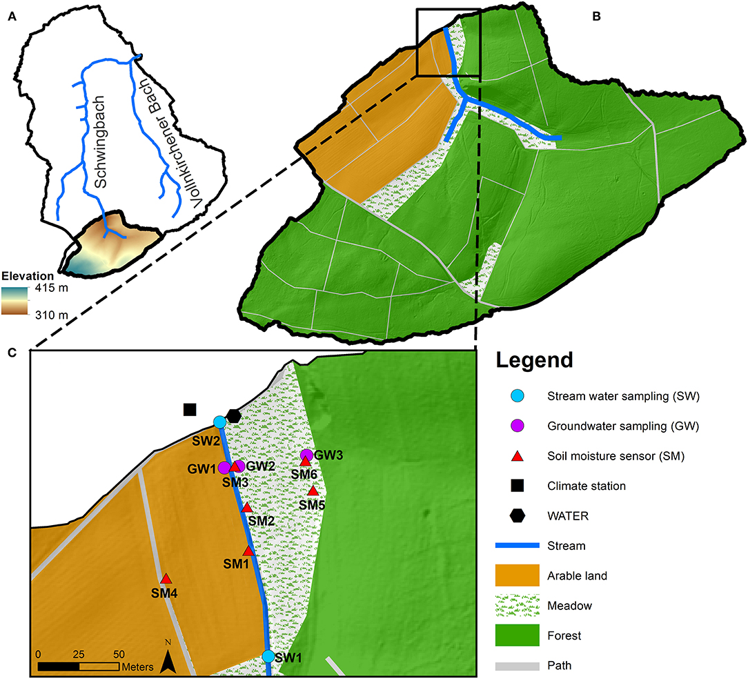
Figure 1. (A) Schwingbach Environmental Observatory (SEO), (B) study area in the Schwingbach headwater and (C) measuring network along the stream reach of the Schwingbach headwater.
An automated climate station (AQ5, Campbell Scientific Inc., Shepshed, UK) equipped with a CR1000 data logger recorded precipitation depth, air temperature, relative humidity, air pressure, solar radiation and wind speed at 5 min intervals (Figure 1C). Six remote-controlled data loggers (A753, Adcon, Klosterneuburg, Austria), three at the toeslope (SM1, SM2 and SM3) and three at the footslope (SM4, SM5 and SM6), were connected to sensors (ECH2O 5TE, METER Environment, Pullman, USA) to automatically monitor soil moisture at 5 and 15 cm depths at 5 min intervals. A stream gauge (RBC flume, Eijkelkamp Agrisearch Equipment, Giesbeek, Netherlands) equipped with a pressure transducer (Mini-Diver, Eigenbrodt Inc., Königsmoor, Germany) automatically measured water levels at the outlet (SW2) of the catchment at 10 min intervals. The transducer measurements were calibrated against manual readings and continuous stream discharge was obtained via the calibrated stage-discharge relationship provided by the manufacturer.
An automated mobile laboratory, the Water Analysis Trailer for the Environmental Research (WATER), was used to automatically sample and analyse the stable isotopes of water (δ2H and δ18O), water temperature, potential of hydrogen (pH) and electrical conductivity (EC) for multiple water sources in situ from August 8th until December 9th in 2018 and from April 12th until October 10th in 2019. The WATER was equipped with a continuous water sampler (CWS) (A0217, Picarro Inc., Santa Clara, USA), coupled to a wavelength-scanned cavity ring-down spectrometer (WS-CRDS) (L2130-i, Picarro Inc., Santa Clara, USA) to analyse the isotopic composition of sampled water. Isotopic ratios are reported in per mill (‰) deviations from the Vienna Standard Mean Ocean Water (VSMOW). We only used δ2H time series in the LSTM modeling, as δ18O had a similar variation but lower precision (precision 0.23‰ for δ18O and 0.57‰ for δ2H). The high-resolution δ2H data were verified with water samples that were manually collected from the sampling sites on a weekly basis. A multi-parameter water quality probe (YSI600R, YSI Inc., Yellow Springs, USA) was installed on the sampling board of the WATER to measure temperature, pH and EC of sampled water. For a detailed description of the WATER and the sampling setup refer to Sahraei et al. (2020).
We measured the stable isotope composition (δ2H), water temperature, pH and EC of two stream water reaches (SW1 and SW2) and three groundwater sources (GW1, GW2 and GW3) (Figure 1C). SW1 was sampled approximately 145 m upstream of the WATER at the edge of farmland and SW2 was sampled at the outlet of the catchment next to the WATER. Groundwater was sampled from piezometers made from perforated PVC tubes sealed in the upper part with bentonite clay to prevent contamination by surface water. The piezometers of GW1 and GW2 were located at the toeslope on the farmland and meadow, respectively. The piezometer of GW3 was located at the footslope at the edge of the forest. The sampling schedule of the WATER allowed measuring isotopic composition, water temperature, pH and EC for each of the stream water reaches at 1.5-h and for each of the groundwater sources at 3-h intervals.
Data Pre-processing
As the input features for our LSTM model, we selected a set of explanatory data that are more straightforward and less expensive to measure compared to the stable isotopes of water. The input features were categorized into meteorological, catchment wetness and natural tracer variables (Table 1). Our collected data set contained different sampling frequencies. To obtain a uniform frequency, which matches the frequency of the output variable, we aggregated all of the observed data to 3-h intervals by averaging, except the precipitation, which was aggregated to 3-h intervals by summing up. The winter period (10th December 2018–11th April 2019) was excluded from the data set because the WATER did not sample during this period due to the freezing weather conditions. When gaps occurred over small timescales due to faulty sensors or equipment maintenance, we used linear interpolation to estimate the missing values. The proportions of observations, which were gap filled through linear interpolation, accounted for at most 3% (73 observations) of total length of the time series for each of the features. We split the observations of all the features into train (70%, 1,700 observations), validation (15%, 365 observations) and test (15%, 365 observations) sets, while maintaining the temporal order of the observations. The train set was used to learn the internal parameters (i.e., weights and bias) of the model. The validation set was used to optimize the hyperparameter, and the test set was used to evaluate the generalization capability of the model. To stabilize the learning process and to speed up the convergence, the data needs to be normalized before feeding to the model. For this, the train set was normalized to be in the range [0–1]. The validation and test sets were normalized using the parameters obtained from the train set normalization to avoid data leakage (Hastie et al., 2009).
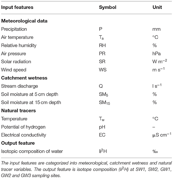
Table 1. Input and output features.
Long Short-Term Memory (LSTM) Model
The LSTM is a type of a Recurrent Neural Network (RNN) that is capable of learning long-term dependencies by overcoming the exploding and vanishing gradient problems of traditional RNN networks (Hochreiter and Schmidhuber, 1997). The main characteristics of the LSTM are the specially designed units so called memory cell and gates. The memory cell consists of forget, input and output gates that together control the flow of information within the LSTM network. The structure of the LSTM memory cell and the algorithms in the cell are shown in Figure 2. The memory cell contains a specific status for each time step, the so-called cell state c, which contains the information for long-term memory. The forget gate controls which information is removed from the cell state. The input gate defines which information is updated to the cell state and the output gate specifies which information is used from the cell state. Suppose a sequence of inputs x = [x1, . .., xT] with T time steps, where each element xt is a vector that contains input at time step (1 ≤ t ≤ T), the process within the LSTM cell is represented with the equations 1–6. The LSTM cell updates six parameters at each time step. The first parameter is the forget gate parameter ft that decides how much of the information from the previous cell state ct−1 needs to be forgotten by a sigmoid function (σ) with a linear calculation of the current input xt and the previous output ht−1. W's and b's with different subscripts represent the gate-specific network weights and bias parameters for the linear calculations. The second parameter is the input gate parameter it that controls which new information is updated to the cell state by the sigmoid function with a linear relation on xt and ht−1 as well. The new cell state candidate ct′ is calculated by a hyperbolic tangent function (tanh) with a linear relation on xt and ht−1. The cell state ct is then updated through an element-wise multiplication ⊙ operator. In the end, the output parameter ot is calculated by the sigmoid function with a linear relation on xt and ht−1. The final output at the current time step ht is the production of ot and the tanh function value of the cell state ct.
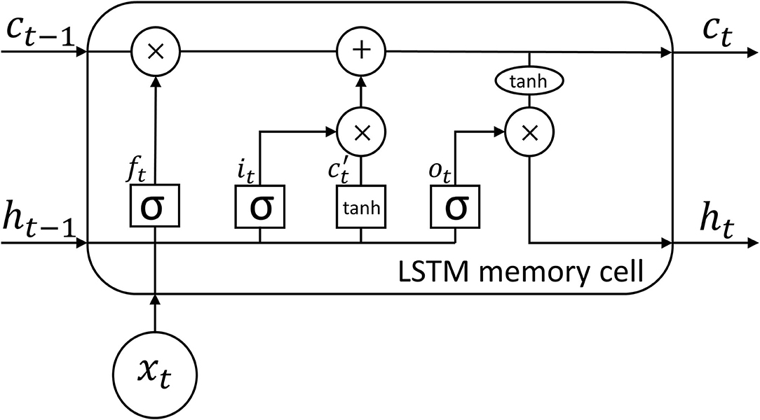
Figure 2. The architecture of LSTM memory cell.
Hyperparameter Optimization
The majority of machine learning algorithms possess several settings that control the entire learning process (Goodfellow et al., 2016). These settings are referred to as hyperparameters. The hyperparameters are exterior to the model and need to be set before the learning process (Géron, 2019). The performance and computational complexity of LSTM models strongly depend on the set of hyperparameters that determine many aspects of the algorithm's behavior (Nakisa et al., 2018). Therefore, it is essential to optimize hyperparameters to boost the LSTM performance. In this study, we used a Sequential Model-Based Optimization (SMBO) search with the Tree-structured Parzen Estimator (TPE) algorithm, a Bayesian optimization approach (Bergstra et al., 2011). Bayesian optimization is a very effective optimization algorithm that has been shown to outperform well-established methods i.e., grid and random search (Bergstra et al., 2013; Eggensperger et al., 2013). It develops a statistical model between the hyperparameters and the objective function and makes the assumption that there is a smooth but noisy function that maps between the hyperparameters and the objective function (Reimers and Gurevych, 2017). Given the search history of hyperparameters and objective function, SMBO-TPE suggests hyperparameters for the next trial that are expected to improve the objective function. As the number of trials grows, the search history expands and eventually the hyperparameters become optimized. In this study, we optimized the number of hidden units (i.e., neurons), dropout rate, learning rate, number of epochs and batch size (Table 2). We ran the optimization evaluation for 1,000 trials through the search space of the hyperparameters to minimize mean squared error (MSE) on the validation set. The complete set of optimized hyperparameters can be found in Table S1 in the Supplementary Material.
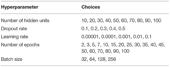
Table 2. Hyperparameter set for the LSTM model.
LSTM Model Setup
The architecture that we used in this study consists of an input layer with as many neurons as input features, one LSTM layer, a dropout layer and a fully connected dense layer with a single unit for the output feature. We used the Adam optimizer for the optimization of the learning process (Kingma and Ba, 2014) and tanh and sigmoid functions as state and gate activation functions, respectively. We ran the LSTM model in a sequence-to-one mode so that an input sequence of a fixed length was used to predict a δ2H value at the next time step. The sequence length, i.e., the look-back window, is the length of past input observations that the LSTM looks back to predict an output for the next time step.
The performance of deep learning models improves by making more training data available (Schmidhuber, 2015). Building a single LSTM model that is trained and optimized on all of the sampling sites instead of training and optimizing a separate LSTM model for each of the sampling sites, allows the network to learn more general and abstract patterns of the input–output relationship (Kratzert et al., 2018). We therefore built a single LSTM model to predict the δ2H values at SW1, SW2, GW1, GW2 and GW3 sampling sites. The LSTM was simultaneously trained on train sets of all sampling sites to learn the internal parameters of the model. It simultaneously used validation sets of all the sampling sites to optimize the hyperparameters and predict the δ2H values on each test set of the sampling sites to estimate the generalization capability of the model.
LSTM Model Sensitivity to Input Features and Sequence Length
We examined how different combinations of input features affect the prediction performance of the LSTM model. It allows us to identify which combinations give us the most accurate predictions of isotope concentrations in the stream and groundwater sampling sites. We tested seven different input feature scenarios shown in Table 3. The first three scenarios (S1, S2 and S3) investigate the effect of meteorological data, catchment wetness conditions and natural tracers on the prediction performance separately. S4, S5 and S6 test the prediction performance when we combine the first three scenarios together and S7 examines the predication performance when we use all of the input features for training of the LSTM. We also used the labels of the sampling sites as input features in all of the seven scenarios. By using the labels of sampling sites as input features, we allow the model to know on which site it trains and hence it produces a unique output for each individual site. This is especially beneficial when using the meteorological data as input features. Since the meteorological data is the same for all sites, the model would otherwise produce the same outputs for them if we do not consider their labels as input features. We used one-hot encoding technique to encode the site labels to the numeric features (Heaton, 2015). This technique creates unique binary columns for each of the labels so that SW1, SW2, GW1, GW2 and GW3 labels are encoded to [1, 0, 0, 0], [0, 1, 0, 0], [0, 0, 1, 0], [0, 0, 0, 1] and [0, 0, 0, 0], respectively. Moreover, we used the month of the year of the measurements' time stamp as an input feature in all seven scenarios to represent the inherent seasonality of the data.
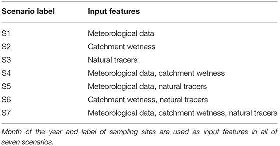
Table 3. Input feature scenarios for the LSTM model.
We also examined the effect of the sequence length of input data on the prediction performance of our LSTM model. The sequence length is intrinsically connected to the underlying physical processes driving the dynamics of output variables (Duan et al., 2020). A proper sequence length should be large enough to incorporate all historical information relevant to the prediction of the isotopic compositions. However, too large sequence lengths increase the model complexity and training time that can in turn reduce the performance (Duan et al., 2020). Some previous studies have set the sequence length to an arbitrary number (Zhang et al., 2018a; Le et al., 2019; Tennant et al., 2020), whereas some other studies have reported that the sequence length affects the model performance (Fan et al., 2020; Meyal et al., 2020; Xiang et al., 2020). We therefore investigated the LSTM sensitivity to the sequence length. We defined nine different sequence lengths into three categories to represent short-, medium- and long-term dependencies. We tested sequence lengths of 6, 12 and 24 h for short-term, 72 (3), 168 (7) and 336 (14) h (days) for medium-term and 720 (30), 1,440 (60) and 2,160 (90) h (days) for long-term dependencies. We examined all of these nine sequence lengths for each of the seven input feature scenarios resulting in 63 different scenarios for the sensitivity analysis. We trained the LSTM model and optimized its hyperparameters for each of these scenarios separately to ensure a fair comparison between them.
Evaluation Metrics
We evaluated the prediction performance of the LSTM model using four statistical metrics (goodness-of-fit criteria). We used root mean squared error (RMSE), mean absolute error (MAE), coefficient of determination (R2) and Nash–Sutcliffe efficiency (NSE) according to equations 7–10.
where N is the number of observations, Oi is the observed value, Pi is the predicted value, is the mean of observed values and is the mean of predicted values. RMSE and MAE explain the average deviation of predicted from observed values with smaller values indicating a better performance. R2 is a good indicator for the temporal correspondence between observed and predicted values ranging between [0–1], with higher values indicating stronger correlations. NSE assesses the model's capability to predict values different from the mean and gives the proportion of the initial variance accounted for by the model (Nash and Sutcliffe, 1970). The NSE is a preferred criterion in many hydrological studies as it particularly describes a model's capability of matching higher values, extremes and outliers. NSE ranges between [–∞ to 1]. The closer the NSE value is to 1, the better is the match between observed and predicted values. A negative value of the NSE denotes that the mean of observed values is a better predictor than the proposed model. Following, Moriasi et al. (2007), model performance can be rated as: very good (0.75 < NSE ≤ 1.00), good (0.65 < NSE ≤ 0.75), satisfactory (0.50 < NSE ≤ 0.65) and unsatisfactory (NSE ≤ 0.50).
Setup of Numerical Experiments
We conducted the numerical experiments with Python 3.7 programming environment (van Rossum, 1995) on Ubuntu 20.04 with AMD EPYC 745-core processor, 125 GB of random access memory (RAM) and NVIDIA GTX 1050 Ti graphical processing unit (GPU). The LSTM model was built with Keras 2.3.1 deep learning framework (Chollet, 2015) on top of TensorFlow backend 2.0 (Abadi et al., 2016). Hyperopt 0.2.5 (Bergstra et al., 2013) and Hyperas 0.4.1 (Pumperla, 2019) libraries were used to implement hyperparameter optimization. Scikit-Learn 0.22.2 (Pedregosa et al., 2011), Pandas 1.0.1 (McKinney, 2010), Numpy 1.18.1 (Van Der Walt et al., 2011), and Scipy 1.4.1 (Virtanen et al., 2020) libraries were used for pre-processing and data management. The Matplotlib 3.1.3 (Hunter, 2007) and Seaborn 0.9.1 (Waskom et al., 2020) libraries were used for the data visualization.
Results and Discussion
Temporal Dynamics
In the following, we briefly describe the dynamics of the observed data over the sampling period (Figures 3–6). During the sampling period of 2018, precipitation is very low with respect to the long-term historical record (Deutscher Wetterdienst, Giessen-Wettenberg station, period 1969-2019, mean annual precipitation of 623 mm), with a total annual precipitation of 452 mm (Figure 3), stating the unusual dry conditions in 2018 (Vogel et al., 2019). More precipitation is observed during the sampling period of 2019 with an annual sum of 624 mm. Air temperature, relative humidity, air pressure, solar radiation and wind speed show strong diurnal fluctuations during the sampling period (Figure 3). However, during the precipitation periods, these fluctuations tend to decrease particularly in case of air temperature and relative humidity, and tend to increase in case of wind speed. Air temperature, relative humidity and solar radiation represent seasonal trends, whereas air pressure and wind speed do not depict a clear trend during the sampling period.
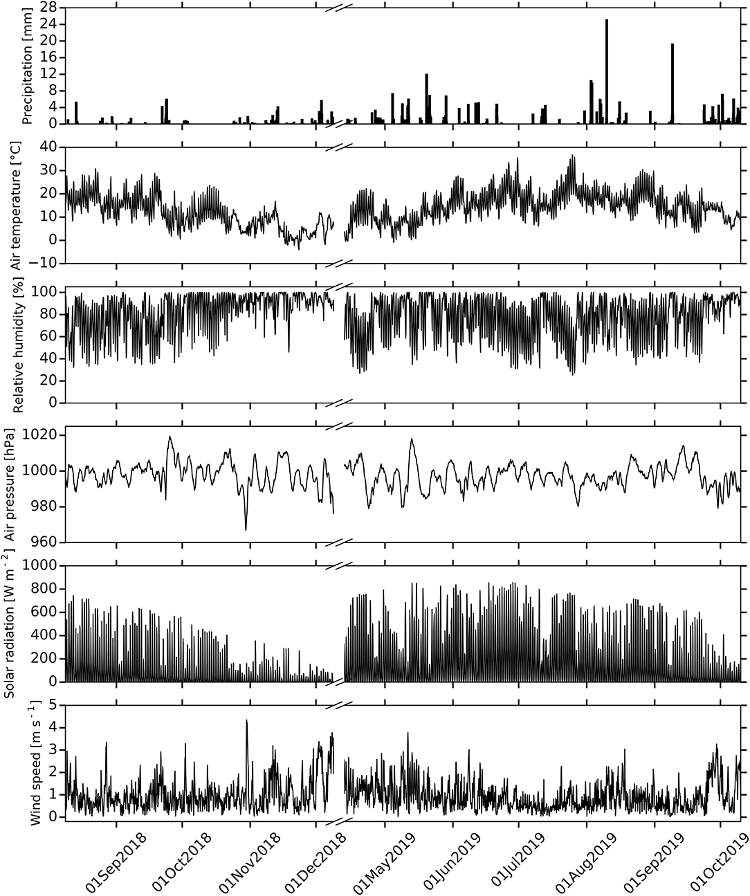
Figure 3. Time series of meteorological data. From the top, we report precipitation, air temperature, relative humidity, air pressure, solar radiation and wind speed.
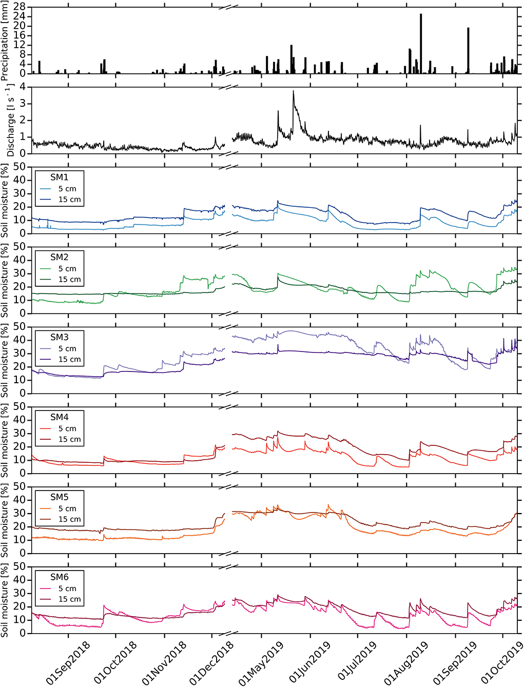
Figure 4. Time series of catchment wetness conditions. From the top, we report precipitation, discharge and soil moisture at SM1, SM2, SM3, SM4, SM5 and SM6 stations.
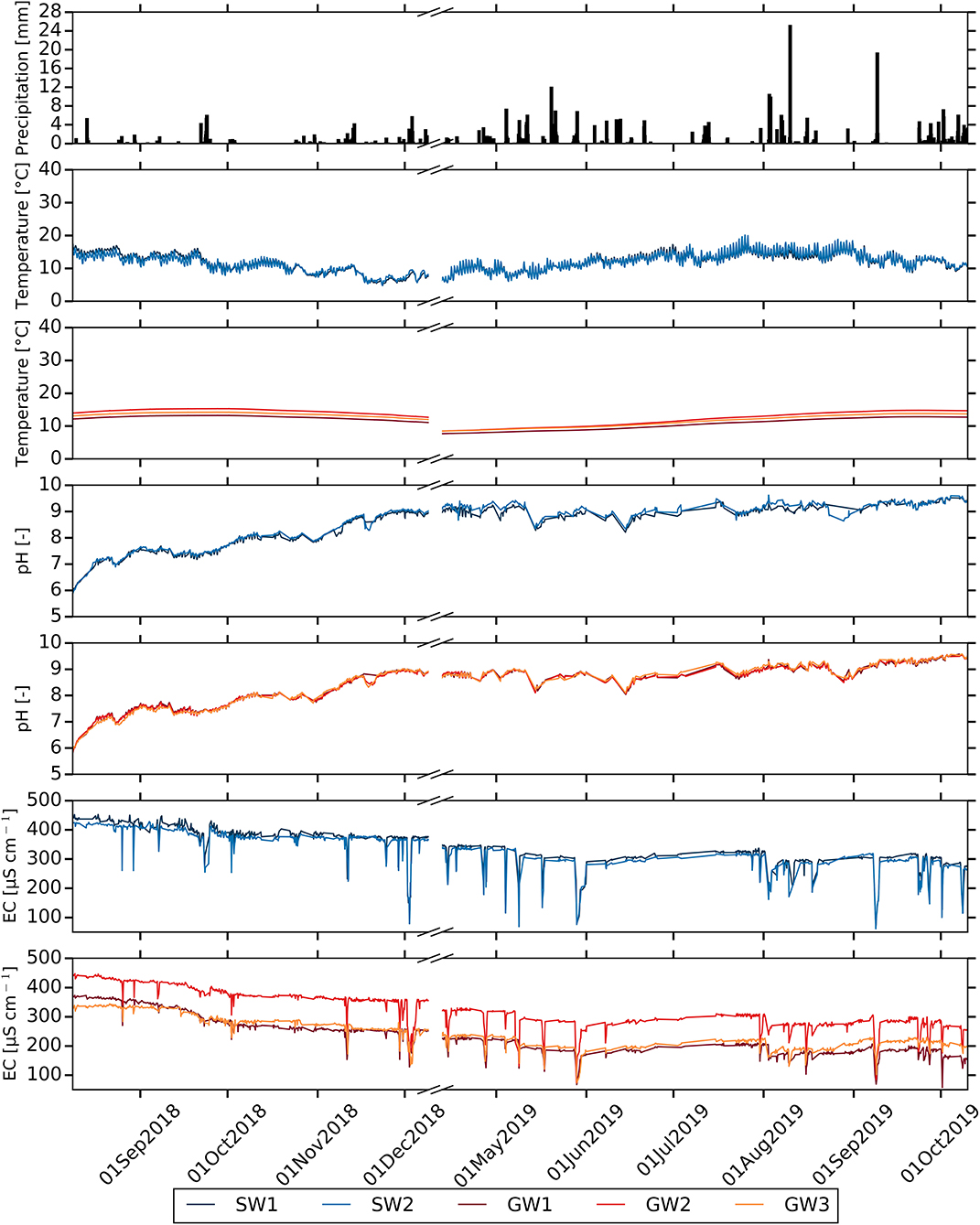
Figure 5. Time series of natural tracers at stream and groundwater sampling sites. From the top, we report precipitation, water temperature, pH and electrical conductivity (EC) at stream and groundwater sampling sites.
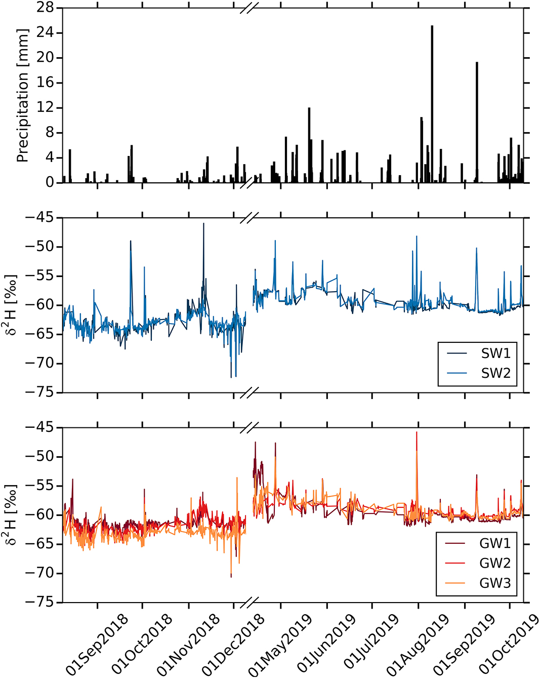
Figure 6. Time series of precipitation and stable isotope concentrations at stream and groundwater sampling sites. From the top, we report, precipitation and δ2H values at stream and groundwater sampling sites.
Stream discharge and soil moisture reflect the drought of 2018 with only few small peaks during the precipitation periods (Figure 4). The catchment wetness increases in 2019 and stream discharge as well as soil moisture react similarly to precipitation inputs. Soil moisture of shallower depth (i.e., 5 cm) generally shows more clear responses to precipitation than at deeper depths (i.e., 15 cm) at all soil moisture stations. This response is more pronounced in the meadow (SM2, SM3 and SM6) than in the farmland (SM1 and SM4). However, soil moisture of deeper depths in the farmland generally reveal a higher responsiveness to rainfall than equivalent depths in the meadow. The shallower depths of SM2 and SM3 at the toeslope depict a similar reaction pattern to SM6 in footslope suggesting the extension of linkage between toeslope and footslope during precipitation events. On average, SM1 and SM3 show the lowest (8 ± 4.3%, mean ± standard deviation, for 5 cm depth, 14 ± 4.6% for 15 cm depth) and highest (29.4 ± 11%, 24.3 ± 6.8%) soil moisture among the SM stations, respectively.
Figure 5 displays that stream water temperature strongly matches the diurnal fluctuations of air temperature, whereas the groundwater temperature follows the overall long-term pattern of air temperature without any high-temporal fluctuations. SW1 and SW2 exhibit similar temperature patterns with means of 11.8 ± 2.7 and 11.7 ± 2.7°C over the sampling period, respectively. However, groundwater temperatures at the sampling sites slightly differs from each other with the mean of 11.3 ± 1.8, 13.0 ± 2.1 and 12.3 ± 1.8°C for GW1, GW2 and GW3, respectively. The patterns of pH dynamics in stream and groundwater sources are almost identical over the sampling period (Figure 5). The pH shows an increasing trend while the air temperature decreases in 2018 and then remains almost stable in 2019 with some fluctuations. The EC of stream and groundwater is highly responsive to precipitation inputs (Figure 5). Rapid reductions of EC are observed upon in the course of precipitation events that are followed by a fast recovery. The EC of stream as well as groundwater is relatively high in 2018, followed by a smooth decline toward the end of the sampling period. The EC of SW1 (336.9 ± 59.3 μS cm−1) is slightly higher than that of SW2 (325.5 ± 58.3 μS cm−1), whereas the difference between the EC of groundwater sampling sites is higher with means of 228.7 ± 61.2, 321.9 ± 59.9 and 239.3 ± 50 μS cm−1 for GW1, GW2 and GW3, respectively.
Figure 6 presents the high temporal resolution of δ2H at the stream and groundwater sampling sites. The δ2H of stream and groundwater responds promptly to precipitation, and is strongly synchronized with the response patterns of EC. These rapid isotopic responses in stream as well as groundwater indicate the strong linkage between stream and subsurface flow pathways during the precipitation events (Sahraei et al., 2020). The δ2H values are lighter with stronger diurnal variations in 2018 compared to those during sampling period of 2019. Seasonal variations are observed during the sampling period with heavier δ2H values in May–June and lighter in November–December. Figure 7 shows the distribution of the isotopic compositions in the stream and groundwater sources over the sampling period. Both stream sampling sites indicate similar variations for δ2H. The mean values of δ2H for SW1 and SW2 are −60.7 ± 2.7‰ and −60.6 ± 2.5‰, respectively. However, the variations of δ2H tend to increase from GW1 to GW3. On average, GW1 (−60.1 ± 2.1‰) and GW2 (−60 ± 1.9‰) at the toeslope depict slightly heavier mean δ2H values compared to GW3 at the footslope (60.5 ± 2.6‰).

Figure 7. Boxplots of the isotopic compositions at stream and groundwater sampling sites. The average is indicated by a black square and the median by the bar separating a box.
LSTM Model Sensitivity to Input Features and Sequence Length
We investigated the impact of input features and sequence length on the prediction performance of the optimized LSTM model. Figure 8 shows the heatmaps of the prediction performance using four statistical metrics for the combination of seven input feature scenarios and nine sequence lengths at the stream and groundwater sampling sites (SW1, SW2, GW1, GW2 and GW3). It is apparent that using the meteorological data (scenario S1) and catchment wetness conditions (scenario S2) alone as the input features does not lead to a good prediction performance. Although using meteorological and catchment wetness data together (scenario S4) slightly decreases prediction errors for some cases, yet the performance is not satisfying. For these scenarios, the NSE values are mainly near to zero and even negative. This emphasizes that the model is not able to predict the peak values properly. It suggests that the relations of meteorological data and catchment wetness variables with the water isotope concentrations are not strong enough to transfer enough information that is required for an adequate learning of the LSTM to predict peak values of isotope concentrations.
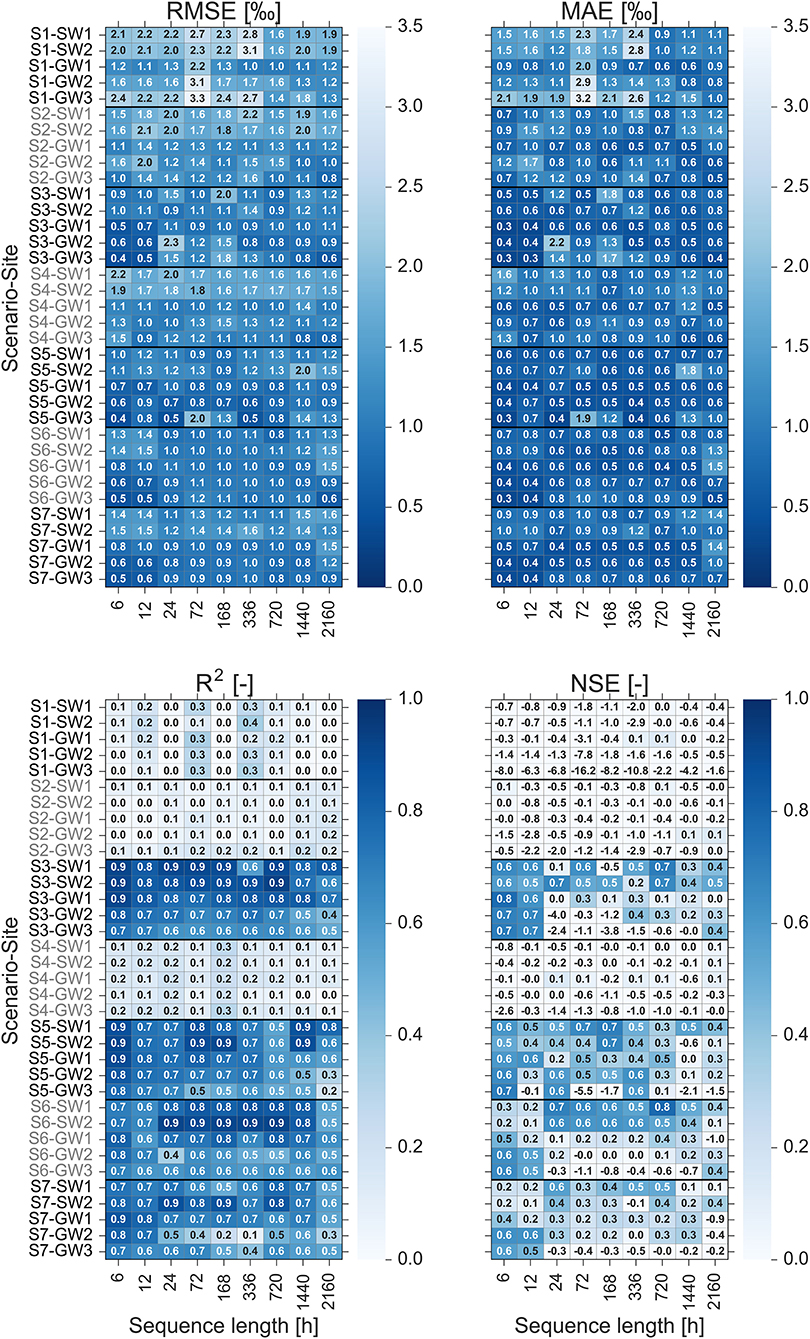
Figure 8. Heatmaps of the prediction performance using four statistical metrics for the combination of seven input feature scenarios and nine sequence lengths at stream and groundwater sampling sites. The dark blue indicates good prediction performance (low values of RMSE and MAE and high values of R2 and NSE), whereas the light blue indicates poor prediction performance (high values of RMSE and MAE and low values of R2 and NSE).
In contrast, using the natural tracers (scenario S3), i.e., water temperature, pH and EC of the sampling sites, as the input features achieves good prediction performance. It indicates that these easy-to-measure tracers are able to indirectly simulate complex interactions between controlling drivers and water isotope concentrations in the Schwingbach catchment. With a closer look to the prediction errors across the sequence lengths of this scenario, we can see that the model performs the best at all of the sampling sites when we use short sequence lengths (6 and 12 h). This implies that the most recent input data contain the most relevant information for the prediction of isotope concentrations and that there is no significant benefit using older input data. This behavior can also be noticed for the prediction of peak values, which is measured by NSE metric. The NSE values are higher for shorter sequence lengths indicating that the model can better predict the reaction of isotope signatures during precipitation events by using the recent input data. This can be associated to the rapid response characteristics of the Schwingbach catchment (Orlowski et al., 2014, 2016; Sahraei et al., 2020). The responses of isotopes in stream and groundwater during precipitation events often reveal a rapid mixing of water at the sampling sites with the event water. It takes, on average, 6 h for stream water and 7–8 h for groundwater at the toeslope (GW1 and GW2) and footslope (GW3), respectively, that the isotope signatures reach peak values. After that, they immediately return to pre-event water conditions (Sahraei et al., 2020). This short-term response behavior together with the synchronized behavior of isotopic compositions with electrical conductivity makes it sufficient for the model to extract the dynamics of isotopic compositions. In contrast, the model performance declines when we use medium and long sequence lengths. This is possibly due to the noise generated by irrelevant inputs (Xiang et al., 2020).
We combined the natural tracers with meteorological and catchment wetness variables (scenarios S5 and S6) to test if this boosts the prediction performance of the LSTM model. Comparing scenario S3 with S5, we can see that the LSTM still performs better at scenario S3 when using short sequence lengths. However, the model tends to perform better at scenario S5 for medium and long sequence lengths. Similarly, the inclusion of catchment wetness (scenario S6) provides some improvements in the model performance for medium and long sequence lengths. The physical explanation underlying the improved performance of the model when we provide longer historical meteorological and catchment wetness information, may be related to the climatological and storage characteristic of the catchment. It could well be that long-term dependencies exist between the dynamics of isotope concentrations and climatic conditions as well as soil water content of the catchment. The ability of the LSTM to learn and remember the long-term dependencies provides the opportunity to identify such storage effects within the catchments (Kratzert et al., 2018, 2019). A comparison between prediction errors of scenario S5 and S6 indicates that the model generally performs better at scenario S5. This suggests that the meteorological condition has a higher impact on the dynamic of isotope concentrations compared to the soil moisture state in the catchment, which is in line with the previous findings in the Schwingbach catchment (Orlowski et al., 2014; Sahraei et al., 2020).
We also tested the prediction performance for all meteorological, catchment wetness and natural tracer variables as input features (scenario S7). In general, the model performance does not improve remarkably and it even deteriorates in some cases compared to performance of model at scenario S3, S5 and S6. The inclusion of too many input features increases the model complexity. Using too complex models augments the chance of overfitting (Maier et al., 2010). Overfitting arises when the model learns the details and noises in the training data to an extent that it is unable to generalize to new data.
Visualization of the LSTM Prediction Performance
We built a single LSTM model to predict the high-resolution δ2H values at SW1, SW2, GW1, GW2 and GW3 sampling sites in the Schwingbach catchment. Ideally, we do not want to train and optimize the model specifically for each sampling site to achieve the best performance, but rather, we intend to train and optimize the model once for all of the sampling sites using only one specific input feature scenario and sequence length. Therefore, we trained and optimized the model with the input feature scenario and sequence length, at which the model performs on average the best for all of the sampling sites. According to the results presented in Figure 8, LSTM achieves the best performance when measurements of the last 6 h of water temperature, pH and EC are used as input features (scenario S3). It achieves, on average of all sampling sites, an RMSE of 0.7‰, MAE of 0.4‰, R2 of 0.9, and NSE of 0.7.
In the following, we visualize the prediction performance of the best LSTM model on the test sets to better illustrate its generalization ability on the unseen data. Figures 9, 10 show the performance of the LSTM using a sequence length of 6 h for scenario S3 at SW1 and GW3 sampling sites, respectively. The LSTM captures the timing of hydrologic events and base flow conditions of δ2H at stream and groundwater sites quite well, but it still underestimates the peak of the hydrograph. This is a commonly known issue with LSTMs and in general, ANN models that they cannot learn adequately the phenomenon in respect of extremes. The major reason that the LSTM may not be able to capture extreme values is the lack of a large number of extremes in the training data (Adnan et al., 2019). The other major reason could be the fact that the range of extreme values in the training data is smaller than those of the validation and test data (Adnan et al., 2019; Malik et al., 2020). This results in difficulties for extrapolation in ANN models (Kisi and Aytek, 2013; Kisi and Parmar, 2016). Several scholars have also reported this limitation in the implementation of the LSTM in previous studies (Kratzert et al., 2018; Chen et al., 2020; Fan et al., 2020; Müller et al., 2020; Xiang et al., 2020). The prediction performances of the best LSTM at SW2, GW1 and GW2 sampling sites are provided in the Supplementary Figures 1–3. The development of the LSTM model assumed stable boundary conditions with regard to land use and cover. Changes of these during the study period have not been taking place in the SEO. However, such changes could be part of long-term simulations in the LSTM model if information were available on this.
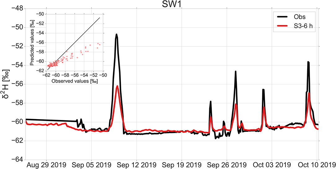
Figure 9. Comparison of observed and predicted δ2H values by the best LSTM using a sequence length of 6 h for water temperature, pH and electrical conductivity measurements (scenario S3-6 h) with an RMSE of 0.9‰, MAE of 0.5‰, R2 of 0.9 and NSE of 0.6 at SW1 site.

Figure 10. Comparison of observed and predicted δ2H values by the best LSTM using a sequence length of 6 h for water temperature, pH and electrical conductivity measurements (scenario S3-6 h) with an RMSE of 0.4‰, MAE of 0.3‰, R2 of 0.7 and NSE of 0.7 at GW3 site.
The power of LSTM as a deep learning model is that it can synthesize information from multiple sampling sites and situations into a single model. An LSTM trained on multiple sites under different landuse and hillslope conditions can learn different patterns of isotopic behavior. It is evident from Figures 9, 10 and Supplementary Figures 1–3 that the LSTM performs efficiently at the stream as well as groundwater sites. Since we trained a single LSTM on stream and groundwater sites with different landuse and hillslope positions with a range of different isotope concentrations and magnitudes of response to precipitation events, the LSTM tends to balance the error so that it minimizes the error between predicted and observed isotope concentrations for all of the sampling sites at the same time. The trained LSTM can be used to spatially estimate the isotope concentrations for multiple sites across the catchment with only simple-to-measure tracers. This leads not only to a substantial reduction of the cost of measurements, but also to an increase in the spatiotemporal knowledge of hydrological processes in the catchment.
One of the challenging tasks in hydrology is the spatial transferability of the models, particularly to data-scarce catchments. Most of hydrological models need to be rebuilt from scratch using newly collected data when the distribution of data is changed in the feature space. However, collecting adequate data is still challenging in many catchments due to the time consuming and expensive measurement procedures. “Transfer learning” is a powerful technique of deep learning that reduces the need and effort to collect the data in data-scarce catchments. Transfer learning is a method that transfers the knowledge obtained in the source domain to the target domain when the latter has few data (Pan and Yang, 2010). Generally, if the deep learning model exhibits satisfying performance in the source catchment, it can be then generalized to target catchments and achieve good prediction performances without much additional data. The transfer learning is efficient in the LSTM because the hidden layers that have been trained to digest shape information, are still effective even when applied to data-scarce catchments (Shen, 2018). In order to apply the proposed LSTM to another catchment, the last fully connected layers are trained on the new data with initial random weights (Yosinski et al., 2014). Although the data is different from the one on which the model is already trained, the low-level features are similar. Therefore, transferring parameters from the “pre-trained LSTM” can provide the new target model with powerful feature extraction ability and reduce the data demand as well as computation or monitoring costs.
The prediction performance of LSTM and in general deep learning models could be enhanced when having more training data available (Schmidhuber, 2015). Providing longer historical data from multiple years for the training process in future research may allow the model to capture long-term seasonal trends under various flow regimes and hydroclimatic conditions, and hence extract more related information that can effectively reproduce the dynamic of the isotope concentrations. It will be particularly interesting to investigate how extreme weather events impact on the LSTM outcome. For the future, we might be able to test this given the current rather wet weather patterns of 2021, which are substantially different to the study period of our current work, which considers rather dry weather conditions from 2018 and 2019.
Conclusion
This study investigates the application of Long Short-Term Memory (LSTM) deep learning model to predict high-resolution (3 h) isotope concentrations of multiple stream and groundwater sources under different landuse and hillslope positions in the Schwingbach Environmental Observatory (SEO), Germany. The core objective of this study is to explore the prediction performance of an LSTM that is trained on multiple sites, with a set of explanatory data that are more straightforward and less expensive to measure compared to the stable isotopes of water. The explanatory data consist of meteorological data, catchment wetness conditions and natural tracers (i.e., water temperature, pH and electrical conductivity). This study further conducts a sensitivity analysis to examine how different input features and their sequence lengths affect the performance of the LSTM. The ability of the LSTM that inherently considers the impact of environmental factors such as evaporation and evapotranspiration on fractionation of water isotopes without an explicit representation of the underlying processes provides the opportunity to efficiently apply the proposed model to isotope hydrology. The result showed that the LSTM could successfully predict stable isotopes of stream and groundwater sites when using only short-term sequence (6 h) of measured water temperature, pH and electrical conductivity. The LSTM prediction can be utilized to predict and interpolate the continuous isotope concentration time series either for data gap filling or in case where no continuous data acquisition is feasible. This is very valuable in practice because measurements of these tracers are still much cheaper than stable isotopes of water and can be continuously carried out with relatively minor maintenance.
For the future research, we will be collecting more data to enhance the prediction performance of the LSTM. There is still room to capture the peak isotope concentrations better. New input features like groundwater table should be used to potentially improve the model performance in the future. The data-hungry nature of deep learning models is a potential barrier for applying them in data-scarce catchments. Since many catchments of potential application may lack the length of the data available in this work, the sensitivity of prediction performance to the length of the training data warrants further investigation. The use of pre-trained LSTM is a promising approach to mitigate the large demand for data in a single catchment. The future research direction also includes applying the LSTM to predict high-resolution water quality parameters such as nitrate, pH and water temperature.
Data Availability Statement
The datasets presented in this study can be found in online repositories. The names of the repository/repositories and accession number(s) can be found below: Zenodo repository, https://doi.org/10.5281/zenodo.5084698.
Author Contributions
AS, TH, and LB conceptualized the research. AS performed data acquisition, data analysis and model development, and prepared the manuscript with contributions from all authors. LB and TH reviewed and revised the manuscript. LB supervised the project. All authors have read and approved the content of the manuscript.
Conflict of Interest
The authors declare that the research was conducted in the absence of any commercial or financial relationships that could be construed as a potential conflict of interest.
Publisher's Note
All claims expressed in this article are solely those of the authors and do not necessarily represent those of their affiliated organizations, or those of the publisher, the editors and the reviewers. Any product that may be evaluated in this article, or claim that may be made by its manufacturer, is not guaranteed or endorsed by the publisher.
Supplementary Material
The Supplementary Material for this article can be found online at: https://www.frontiersin.org/articles/10.3389/frwa.2021.740044/full#supplementary-material
References
Abadi, M., Agarwal, A., Barham, P., Brevdo, E., Chen, Z., Citro, C., et al. (2016). TensorFlow: Large-scale machine learning on heterogeneous distributed systems. arXiv Preprint. Available online at: https://arxiv.org/abs/1603.04467.
Adnan, R. M., Liang, Z., Heddam, S., Zounemat-Kermani, M., Kisi, O., and Li, B. (2019). Least square support vector machine and multivariate adaptive regression splines for streamflow prediction in mountainous basin using hydro-meteorological data as inputs. J. Hydrol. 586:124371. doi: 10.1016/j.jhydrol.2019.124371
Benardos, P. G., and Vosniakos, G. C. (2007). Optimizing feedforward artificial neural network architecture. Eng. Appl. Artif. Intell. 20, 365–382. doi: 10.1016/j.engappai.2006.06.005
Bergstra, J., Bardenet, R., Bengio, Y., and Kégl, B. (2011). Algorithms for hyper-parameter optimization. Adv. Neural Inform. Process. Syst. 24, 1–9.
Bergstra, J., Yamins, D., and Cox, D. D. (2013). “Making a Science of Model Search: Hyperparameter optimization in hundreds of dimensions for vision architectures,” in International Conference on Machine Learning, 115–123.
Berman, E. S. F., Gupta, M., Gabrielli, C., Garland, T., and McDonnell, J. J. (2009). High-frequency field-deployable isotope analyzer for hydrological applications. Water Resour. Res. 45, 1–7. doi: 10.1029/2009WR008265
Birkel, C., Soulsby, C., Tetzlaff, D., Dunn, S., and Spezia, L. (2012). High-frequency storm event isotope sampling reveals time-variant transit time distributions and influence of diurnal cycles. Hydrol. Process. 26, 308–316. doi: 10.1002/hyp.8210
Calkoen, F., Luijendijk, A., Rivero, C. R., Kras, E., and Baart, F. (2021). Traditional vs. Machine-learning methods for forecasting sandy shoreline evolution using historic satellite-derived shorelines. Remote Sens. 13, 1–21. doi: 10.3390/rs13050934
Cerar, S., Mezga, K., Žibret, G., Urbanc, J., and Komac, M. (2018). Comparison of prediction methods for oxygen-18 isotope composition in shallow groundwater. Sci. Total Environ. 631–632, 358–368. doi: 10.1016/j.scitotenv.2018.03.033
Chen, X., Huang, J., Han, Z., Gao, H., Liu, M., Li, Z., et al. (2020). The importance of short lag-time in the runoff forecasting model based on long short-term memory. J. Hydrol. 589:125359. doi: 10.1016/j.jhydrol.2020.125359
Chollet, F. (2015). Keras. Available online at: https://keras.io (accessed August 25, 2021).
Duan, S., Ullrich, P., and Shu, L. (2020). Using convolutional neural networks for streamflow projection in California. Front. Water 2:28. doi: 10.3389/frwa.2020.00028
Eggensperger, K., Feurer, M., Hutter, F., Bergstra, J., Snoek, J., Holger, H., et al. (2013). “Towards an empirical foundation for assessing bayesian optimization of hyperparameters,” in NIPS Workshop on Bayesian Optimazation in Theory and Practice, vol 10, 3.
Fan, H., Jiang, M., Xu, L., Zhu, H., Cheng, J., and Jiang, J. (2020). Comparison of long short term memory networks and the hydrological model in runoff simulation. Water 12, 1–17. doi: 10.3390/w12010175
Fang, K., Shen, C., Kifer, D., and Yang, X. (2017). Prolongation of SMAP to spatiotemporally seamless coverage of continental U.S. using a deep learning neural network. Geophys. Res. Lett. 44, 11,030–11,039. doi: 10.1002/2017GL075619
Géron, A. (2019). Hands-On Machine Learning With Scikit-Learn, Keras, And TensorFlow: Concepts, Tools, And Techniques To Build Intelligent Systems. Sebastopol, CA: O'Reilly Media.
Gers, F. A., Eck, D., and Schmidhuber, J. (2002). “Applying LSTM to time series predictable through time-window approaches,” in Neural Nets WIRN Vietri-01 (London: Springer), 193–200. doi: 10.1007/978-1-4471-0219-9_20
Hastie, T., Tibshirani, R., and Friedman, J. (2009). The Elements of Statistical Learning: Data Mining, Inference, and Prediction. New York, NY: Springer Science and Business Media. doi: 10.1007/978-0-387-84858-7
Heaton, J. (2015). Artificial Intelligence for Humans, Volume 3: Deep Learning and Neural Networks. Chesterfield, MO: Heaton Research, Inc.
Heinz, E., Kraft, P., Buchen, C., Frede, H.-G., Aquino, E., and Breuer, L. (2014). Set up of an automatic water quality sampling system in irrigation agriculture. Sensors 14, 212–228. doi: 10.3390/s140100212
Hochreiter, S., and Schmidhuber, J. (1997). Long short-term memory. Neural Comput. 9, 1735–1780. doi: 10.1162/neco.1997.9.8.1735
Hunter, J. D. (2007). Matplotlib: A 2D graphics environment. IEEE Ann. Hist. Comput. 9, 90–95. doi: 10.1109/MCSE.2007.55
Kendall, C., and McDonnell, J. J. (2012). Isotope Tracers in Catchment Hydrology. Amsterdam: Elsevier.
Khashei, M., and Bijari, M. (2010). An artificial neural network (p, d, q) model for timeseries forecasting. Expert Syst. Appl. 37, 479–489. doi: 10.1016/j.eswa.2009.05.044
Khashei, M., Bijari, M., and Raissi Ardali, G. A. (2009). Improvement of auto-regressive integrated moving average models using fuzzy logic and Artificial Neural Networks (ANNs). Neurocomputing 72, 956–967. doi: 10.1016/j.neucom.2008.04.017
Kingma, D. P., and Ba, J. L. (2014). Adam: a method for stochastic optimization. arXiv Preprint Available online at: https://arxiv.org/abs/1412.6980.
Kisi, O., and Aytek, A. (2013). Explicit neural network in suspended sediment load estimation. Neural Netw. World 23, 587–607. doi: 10.14311/NNW.2013.23.035
Kisi, O., and Parmar, K. S. (2016). Application of least square support vector machine and multivariate adaptive regression spline models in long term prediction of river water pollution. J. Hydrol. 534, 104–112. doi: 10.1016/j.jhydrol.2015.12.014
Klaus, J., and McDonnell, J. J. (2013). Hydrograph separation using stable isotopes: review and evaluation. J. Hydrol. 505, 47–64. doi: 10.1016/j.jhydrol.2013.09.006
Koeniger, P., Gaj, M., Beyer, M., and Himmelsbach, T. (2016). Review on soil water isotope-based groundwater recharge estimations. Hydrol. Process. 30, 2817–2834. doi: 10.1002/hyp.10775
Kratzert, F., Klotz, D., Brenner, C., Schulz, K., and Herrnegger, M. (2018). Rainfall-runoff modelling using Long Short-Term Memory (LSTM) networks. Hydrol. Earth Syst. Sci. 22, 6005–6022. doi: 10.5194/hess-22-6005-2018
Kratzert, F., Klotz, D., Shalev, G., Klambauer, G., Hochreiter, S., and Nearing, G. (2019). Towards learning universal, regional, and local hydrological behaviors via machine learning applied to large-sample datasets. Hydrol. Earth Syst. Sci. 23, 5089–5110. doi: 10.5194/hess-23-5089-2019
Lange, H., and Sippel, S. (2020). “Machine learning applications in hydrology,” in Forest-Water Interactions, eds. D. F. Levia, D. E. Carlyle-Moses, S. Iida, and B. Michalzik (Cham: Springer), 233–257. doi: 10.1007/978-3-030-26086-6_10
Le, X., Ho, H. V., Lee, G., and Jung, S. (2019). Application of Long Short-Term Memory (LSTM) neural network for flood forecasting. Water 11:1387. doi: 10.3390/w11071387
Liu, P., Wang, J., Sangaiah, A., Xie, Y., and Yin, X. (2019). Analysis and prediction of water quality using LSTM deep neural networks in IoT environment. Sustainability 11:2058. doi: 10.3390/su11072058
Mahindawansha, A., Breuer, L., Chamorro, A., and Kraft, P. (2018). High-frequency water isotopic analysis using an automatic water sampling system in rice-based cropping systems. Water 10:1327. doi: 10.3390/w10101327
Maier, H. R., and Dandy, G. C. (2000). Neural networks for the prediction and forecasting of water resources variables: a review of modelling issues and applications. Environ. Model. Softw. 15, 101–124. doi: 10.1016/S1364-8152(99)00007-9
Maier, H. R., Jain, A., Dandy, G. C., and Sudheer, K. P. (2010). Methods used for the development of neural networks for the prediction of water resource variables in river systems: current status and future directions. Environ. Model. Softw. 25, 891–909. doi: 10.1016/j.envsoft.2010.02.003
Malik, A., Tikhamarine, Y., Souag-Gamane, D., Kisi, O., and Pham, Q. B. (2020). Support vector regression optimized by meta-heuristic algorithms for daily streamflow prediction. Stoch. Environ. Res. Risk Assess. 34, 1755–1773. doi: 10.1007/s00477-020-01874-1
McGlynn, B. L., McDonnell, J. J., Seibert, J., and Kendall, C. (2004). Scale effects on headwater catchment runoff timing, flow sources, and groundwater-streamflow relations. Water Resour. Res. 40. doi: 10.1029/2003WR002494
McGuire, K. J., and McDonnell, J. J. (2006). A review and evaluation of catchment transit time modeling. J. Hydrol. 330, 543–563. doi: 10.1016/j.jhydrol.2006.04.020
McKinney, W. (2010). “Data structures for statistical computing in python,” in Proceedings of the 9th Python in Science Conference (Austin, TX), 56–61. doi: 10.25080/Majora-92bf1922-00a
Meyal, A. Y., Versteeg, R., Alper, E., and Johnson, D. (2020). Automated cloud based long short-term memory neural network based SWE prediction. Front. Water 2:574917. doi: 10.3389/frwa.2020.574917
Moriasi, D. N., Arnold, J. G., Van Liew, M. W., Bingner, R. L., Harmel, R. D., and Veith, T. L. (2007). Model evaluation guidelines for systematic quantification of accuracy in watershed simulations. Trans. Am. Soc. Agric. Biol. Eng. 50, 885–900. doi: 10.13031/2013.23153
Müller, J., Park, J., Sahu, R., Varadharajan, C., Arora, B., Faybishenko, B., et al. (2020). Surrogate optimization of deep neural networks for groundwater predictions. J. Glob. Optim. 81, 203–231. doi: 10.1007/s10898-020-00912-0
Nakisa, B., Rastgoo, M. N., Rakotonirainy, A., Maire, F., and Chandran, V. (2018). Long short term memory hyperparameter optimization for a neural network based emotion recognition framework. IEEE Access 6, 49325–49338. doi: 10.1109/ACCESS.2018.2868361
Nash, J. E., and Sutcliffe, J. V. (1970). River flow forecasting through conceptual models part I—A discussion of principles. J. Hydrol. 10, 282–290. doi: 10.1016/0022-1694(70)90255-6
Orlowski, N., Kraft, P., Pferdmenges, J., and Breuer, L. (2016). Exploring water cycle dynamics by sampling multiple stable water isotope pools in a developed landscape in Germany. Hydrol. Earth Syst. Sci. 20, 3873–3894. doi: 10.5194/hess-20-3873-2016
Orlowski, N., Lauer, F., Kraft, P., Frede, H. G., and Breuer, L. (2014). Linking spatial patterns of groundwater table dynamics and streamflow generation processes in a small developed catchment. Water 6, 3085–3117. doi: 10.3390/w6103085
Pan, S. J., and Yang, Q. (2010). A survey on transfer learning. IEEE Trans. Knowl. Data Eng. 22, 1345–1359. doi: 10.1109/TKDE.2009.191
Pedregosa, F., Varoquaux, G., Gramfort, A., Michel, V., Thirion, B., Grisel, O., et al. (2011). Scikit-learn: machine learning in python. J. Mach. Learn. Res. 12, 2825–2830.
Pumperla, M. (2019). Hyperas. Available online at: https://pypi.org/project/hyperas/ (accessed May 10, 2021).
Quade, M., Klosterhalfen, A., Graf, A., Brüggemann, N., Hermes, N., Vereecken, H., et al. (2019). In-situ monitoring of soil water isotopic composition for partitioning of evapotranspiration during one growing season of sugar beet (Beta vulgaris). Agric. For. Meteorol. 266–267, 53–64. doi: 10.1016/j.agrformet.2018.12.002
Reimers, N., and Gurevych, I. (2017). Optimal hyperparameters for deep LSTM-networks for sequence labeling tasks. arXiv Preprint. Available online at: https://arxiv.org/abs/1707.06799.
Sahraei, A., Chamorro, A., Kraft, P., and Breuer, L. (2021). Application of machine learning models to predict maximum event water fractions in streamflow. Front. Water 3:652100. doi: 10.3389/frwa.2021.652100
Sahraei, A., Kraft, P., Windhorst, D., and Breuer, L. (2020). High-resolution, in situ monitoring of stable isotopes of water revealed insight into hydrological behavior. Water 12:565. doi: 10.3390/w12020565
Samuel, A. L. (1959). Some studies in machine learning using the game of checkers. IBM J. Res. Dev. 3, 210–299. doi: 10.1147/rd.33.0210
Schmidhuber, J. (2015). Deep Learning in neural networks: an overview. Neural Netw. 61, 85–117. doi: 10.1016/j.neunet.2014.09.003
Shen, C. (2018). A transdisciplinary review of deep learning research and its relevance for water resources scientists. Water Resour. Res. 54, 8558–8593. doi: 10.1029/2018WR022643
Sprenger, M., Leistert, H., Gimbel, K., and Weiler, M. (2016). Illuminating hydrological processes at the soil-vegetation- atmosphere interface with water stable isotopes. Rev. Geophys. 54, 674–704. doi: 10.1002/2015RG000515
Tennant, C., Larsen, L., Bellugi, D., Moges, E., Zhang, L., and Ma, H. (2020). The utility of information flow in formulating discharge forecast models: a case study from an arid snow-dominated catchment. Water Resour. Res. 56, 1–21. doi: 10.1029/2019WR024908
Tetzlaff, D., Buttle, J., Carey, S. K., Mcguire, K., Laudon, H., and Soulsby, C. (2015). Tracer-based assessment of flow paths, storage and runoff generation in northern catchments: a review. Hydrol. Process. 29, 3475–3490. doi: 10.1002/hyp.10412
Uhlenbrook, S., Frey, M., Leibundgut, C., and Maloszewski, P. (2002). Hydrograph separations in a mesoscale mountainous basin at event and seasonal timescales. Water Resour. Res. 38, 31-1–31-14. doi: 10.1029/2001WR000938
Van Der Walt, S., Colbert, S. C., and Varoquaux, G. (2011). The NumPy array: a structure for efficient numerical computation. Comput. Sci. Eng. 13, 22–30. doi: 10.1109/MCSE.2011.37
Virtanen, P., Gommers, R., Oliphant, T. E., Haberland, M., Reddy, T., Cournapeau, D., et al. (2020). SciPy 1.0: fundamental algorithms for scientific computing in Python. Nat. Methods 17, 261–272. doi: 10.1038/s41592-019-0686-2
Vogel, M. M., Zscheischler, J., Wartenburger, R., Dee, D., and Seneviratne, S. I. (2019). Concurrent 2018 hot extremes across northern hemisphere due to human-induced climate change. Earth's Futur. 7, 692–703. doi: 10.1029/2019EF001189
von Freyberg, J., Studer, B., and Kirchner, J. W. (2017). A lab in the field: high-frequency analysis of water quality and stable isotopes in stream water and precipitation. Hydrol. Earth Syst. Sci. 21, 1721–1739. doi: 10.5194/hess-21-1721-2017
Waskom, M., Botvinnik, O., Gelbart, M., Ostblom, J., Hobson, P., Lukauskas, S., et al. (2020). Seaborn: statistical data visualization. Astrophys. Source Code Libr. 1–4. doi: 10.5281/zenodo.592845
Windhorst, D., Kraft, P., Timbe, E., Frede, H. G., and Breuer, L. (2014). Stable water isotope tracing through hydrological models for disentangling runoff generation processes at the hillslope scale. Hydrol. Earth Syst. Sci. 18, 4113–4127. doi: 10.5194/hess-18-4113-2014
Wissmeier, L., and Uhlenbrook, S. (2007). Distributed, high-resolution modelling of 18O signals in a meso-scale catchment. J. Hydrol. 332, 497–510. doi: 10.1016/j.jhydrol.2006.08.003
Xiang, Z., Yan, J., and Demir, I. (2020). A rainfall-runoff model with LSTM-based sequence-to-sequence learning. Water Environ. Res. 56. doi: 10.1029/2019WR025326
Yosinski, J., Clune, J., Bengio, Y., and Lipson, H. (2014). How transferable are features in deep neural networks? arXiv Preprint. Available online at: https://arxiv.org/abs/1411.1792.
Zhang, D., Lin, J., Peng, Q., Wang, D., Yang, T., Sorooshian, S., et al. (2018a). Modeling and simulating of reservoir operation using the artificial neural network, support vector regression, deep learning algorithm. J. Hydrol. 565, 720–736. doi: 10.1016/j.jhydrol.2018.08.050
Zhang, G., Eddy Patuwo, B. Y., and Hu, M. (1998). Forecasting with artificial neural networks: the state of the art. Int. J. Forecast. 14, 35–62. doi: 10.1016/S0169-2070(97)00044-7
Zhang, J., Zhu, Y., Zhang, X., Ye, M., and Yang, J. (2018b). Developing a Long Short-Term Memory (LSTM) based model for predicting water table depth in agricultural areas. J. Hydrol. 561, 918–929. doi: 10.1016/j.jhydrol.2018.04.065
Zhou, J., Liu, G., Meng, Y., Xia, C., Chen, K., and Chen, Y. (2021). Using stable isotopes as tracer to investigate hydrological condition and estimate water residence time in a plain region, Chengdu, China. Sci. Rep. 11:2812. doi: 10.1038/s41598-021-82349-3
Zounemat-Kermani, M., Matta, E., Cominola, A., Xia, X., Zhang, Q., Liang, Q., et al. (2020). Neurocomputing in surface water hydrology and hydraulics: a review of two decades retrospective, current status and future prospects. J. Hydrol. doi: 10.1016/j.jhydrol.2020.125085
Keywords: machine learning, deep learning, long short-term memory, sensitivity analysis, Bayesian hyperparameter optimization, stable isotopes of water, high-resolution data, isotope hydrology
Citation: Sahraei A, Houska T and Breuer L (2021) Deep Learning for Isotope Hydrology: The Application of Long Short-Term Memory to Estimate High Temporal Resolution of the Stable Isotope Concentrations in Stream and Groundwater. Front. Water 3:740044. doi: 10.3389/frwa.2021.740044
Received: 12 July 2021; Accepted: 19 August 2021;
Published: 10 September 2021.
Edited by:
Scott Thomas Allen, University of Nevada, Reno, United StatesReviewed by:
Catie Finkenbiner, Oregon State University, United StatesSi-Liang Li, Tianjin University, China
Copyright © 2021 Sahraei, Houska and Breuer. This is an open-access article distributed under the terms of the Creative Commons Attribution License (CC BY). The use, distribution or reproduction in other forums is permitted, provided the original author(s) and the copyright owner(s) are credited and that the original publication in this journal is cited, in accordance with accepted academic practice. No use, distribution or reproduction is permitted which does not comply with these terms.
*Correspondence: Amir Sahraei, YW1pcmhvc3NlaW4uc2FocmFlaUB1bXdlbHQudW5pLWdpZXNzZW4uZGU=