What Do P-Wave Velocities Tell Us About the Critical Zone?

Flinchum, Brady A.; Holbrook, W. Steven; Carr, Bradley J.

doi:10.3389/frwa.2021.772185

ORIGINAL RESEARCH article

Front. Water, 10 January 2022

Sec. Water and Critical Zone

Volume 3 - 2021 | https://doi.org/10.3389/frwa.2021.772185

This article is part of the Research Topic Critical Zone Geophysics View all 8 articles

What Do P-Wave Velocities Tell Us About the Critical Zone?

$\nBrady A. Flinchum$ Brady A. Flinchum¹^*

W. Steven Holbrook²

Bradley J. Carr³

¹Clemson University, Environmental Engineering and Earth Sciences, Clemson, SC, United States
²Department of Geosciences, Virginia Polytechnic Institute and State University, Blacksburg, VA, United States
³Department of Geology and Geophysics, University of Wyoming, Laramie, WY, United States

Fractures in Earth's critical zone influence groundwater flow and storage and promote chemical weathering. Fractured materials are difficult to characterize on large spatial scales because they contain fractures that span a range of sizes, have complex spatial distributions, and are often inaccessible. Therefore, geophysical characterizations of the critical zone depend on the scale of measurements and on the response of the medium to impulses at that scale. Using P-wave velocities collected at two scales, we show that seismic velocities in the fractured bedrock layer of the critical zone are scale-dependent. The smaller-scale velocities, derived from sonic logs with a dominant wavelength of ~0.3 m, show substantial vertical and lateral heterogeneity in the fractured rock, with sonic velocities varying by 2,000 m/s over short lateral distances (~20 m), indicating strong spatial variations in fracture density. In contrast, the larger-scale velocities, derived from seismic refraction surveys with a dominant wavelength of ~50 m, are notably slower than the sonic velocities (a difference of ~3,000 m/s) and lack lateral heterogeneity. We show that this discrepancy is a consequence of contrasting measurement scales between the two methods; in other words, the contrast is not an artifact but rather information—the signature of a fractured medium (weathered/fractured bedrock) when probed at vastly different scales. We explore the sample volumes of each measurement and show that surface refraction velocities provide reliable estimates of critical zone thickness but are relatively insensitive to lateral changes in fracture density at scales of a few tens of meters. At depth, converging refraction and sonic velocities likely indicate the top of unweathered bedrock, indicative of material with similar fracture density across scales.

Introduction

Interactions among Earth's atmosphere, biosphere, and hydrosphere drive chemical and physical processes that, over geologic time, convert bedrock into soil. These processes create and maintain a structure that extends from Earth's surface vegetation to subsurface depths where bedrock is no longer physically or chemically altered by near-surface processes. This thin region, which supports virtually all terrestrial life, is referred to as Earth's critical zone (CZ) (Richter et al., 2009; Brantley et al., 2017; Riebe et al., 2017). In eroding landscapes, the CZ is conceptualized as layers of soil, saprolite, fractured bedrock, and less altered bedrock (Figure 1). The spatial distribution and characteristics of each of these layers provide valuable information about the processes involved in the weathering of rocks (Anderson et al., 2007; St. Clair et al., 2015; Rempe and Dietrich, 2018), the generation of porosity (Graham et al., 1997; Navarre-Sitchler et al., 2015; Hayes et al., 2019), and water movement in landscapes (Salve et al., 2012; Brooks et al., 2015; Lovill et al., 2018).

FIGURE 1

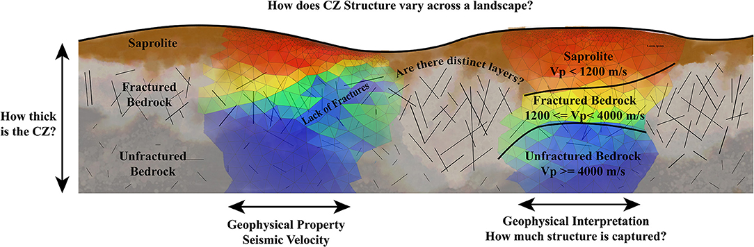
Figure 1. Conceptual drawing of the CZ showing how complexity translates into the smooth velocity images produced with seismic refraction. In CZ studies we represent the complex CZ as discrete elements of a specific physical property—in this case seismic velocity. This figure highlights the challenge of representing complex CZ structure as velocity profiles. A key to utilizing seismic refraction in CZ studies is understanding the scale over which seismic refraction velocities are measured.

Many hypotheses that explain CZ evolution have grown out of observing and understanding the existing architecture of the CZ (Figure 1) (e.g., Riebe et al., 2017). Fundamental questions about CZ architecture remain incompletely answered, including: (1) How thick is the CZ? (2) Are there distinct layers and boundaries within the CZ? (3) If so, how deep are they, how well-defined are they, and how do they vary spatially across a landscape? The answers to these questions will provide crucial tests of hypotheses about the processes that form and maintain the CZ. For example, the interaction between topographic and compressive regional tectonic stresses may control the opening of subsurface fractures, leading to inverted bedrock topography under some hillslopes (Slim et al., 2015; St. Clair et al., 2015; Moon et al., 2017). CZ structure may depend strongly on strong contrasts in hydrogeologic properties such as porosity or hydraulic conductivity (Dralle et al., 2018; Rempe and Dietrich, 2018; Hahm et al., 2019). In some locations, lithologic fabric or foliation (Novitsky et al., 2018; Leone et al., 2020), composition (Hahm et al., 2014; Buss et al., 2017) or geochemical reaction rates (Dixon and Thorn, 2005; Gabet and Mudd, 2009; Hilley et al., 2010; Braun et al., 2016) may control CZ structure and evolution. Testing any of these process-based hypotheses about CZ evolution, or developing new hypotheses, requires quantifying CZ architecture over large areas.

Quantifying CZ architecture requires both drilling and geophysics and must balance inevitable tradeoffs between detail and scale. Soil pits provide detailed, high-resolution information about the top 1–3 m of the CZ (Richter and Markewitz, 1995; Fletcher et al., 2006; Graham et al., 2010), including root distributions (Canadell et al., 1996; Pawlik et al., 2016; Hasenmueller et al., 2017) and water infiltration (Vereecken et al., 2007; Bales et al., 2011; Carey et al., 2019; Kotikian et al., 2019). Road cuts and outcrops provide a detailed look at the CZ (Dethier and Lazarus, 2006; Dewandel et al., 2006; Goodfellow et al., 2014) over larger scales than soil pits, but their locations are not always convenient for testing hypotheses. In contrast, boreholes, although spatially limited, provide in situ windows into deep regions of CZ at high vertical resolution. Boreholes create unique and detailed measurements of the physical structure and chemical composition of the CZ, including fracture density and orientations (Anderson et al., 2002; Kuntz et al., 2011; Holbrook et al., 2019; Gu et al., 2020b), geochemical reactions (Brantley and White, 2009; Brantley et al., 2013; Holbrook et al., 2019), and hydrogeologic properties like porosity and hydraulic conductivity (Walsh et al., 2013; Flinchum et al., 2018a; Ren et al., 2019). A major challenge in CZ science is to obtain measurements that have both high spatial resolution and cover large areas.

Geophysical methods are a tool for exploring deep CZ structure at landscape (1,000s of m) and watershed (10s−100s of m) scales. Near-surface geophysical methods have variable resolution and depth penetration and have been successfully used to quantify lateral and vertical variability in CZ structure (Befus et al., 2011; Leopold et al., 2013; Orlando et al., 2016), estimate bedrock fracture density (Clarke and Burbank, 2011; Golebiowski et al., 2016; Novitsky et al., 2018), and estimate the depth to bedrock (Nyquist et al., 1996; Yaede et al., 2015; Flinchum et al., 2018b; Moravec et al., 2020). Given the diversity of near-surface geophysical methods (e.g., Parsekian et al., 2015), it is critical to select the appropriate geophysical tool to test a given scientific hypothesis. It is also critical to understand how the geophysical properties are related to the underlying physical properties that define CZ structure (Figure 1).

Seismic refraction is a geophysical method that is being increasingly used to study the deeper regions of the CZ (Befus et al., 2011; Olyphant et al., 2016; Callahan et al., 2020; Moravec et al., 2020). Seismic refraction uses elastic energy to produce 2D images of P-wave velocity on the order of 10s−100s of meters per deployment. P-wave velocity is a geophysical property that describes how fast compressional waves travel through a material. P-waves propagate by successively compressing and dilating the material through which they pass (e.g., Pride, 2005). Those compressions and dilatations are strains that occur at the scale of the seismic wavelength: that is, a long-wavelength wave strains a larger volume than a short-wavelength wave, as governed by the universal wave equation, v = λf where v is velocity, λ is wavelength, and f is frequency.

Seismic refraction methods are advantageous for CZ studies because (1) data can be collected quickly with a small team over large scales in rugged terrain; (2) the method quantifies P-wave velocity over 100s of meters; (3) P-wave velocity near Earth's surface is primarily controlled by porosity, a parameter highly relevant to CZ science; (4) the technique provides P-wave velocity estimates to depths of ~50 m or deeper, covering the full depth of the CZ in most areas; and (5) inversions can be run on laptop and desktop computers (Holbrook et al., 2014; Olyphant et al., 2016; Flinchum et al., 2018b; Seyfried et al., 2018; West et al., 2019).

The growing number of studies using seismic velocities to explore the deep CZ make it important for CZ scientists to understand what P-wave velocities can tell us about the CZ. In this paper, we focus on an apparent discrepancy between P-wave velocities collected via seismic refraction using a sledgehammer source (wavelengths of 10s of meters) and P-wave velocities collected from a sonic logging tool at multiple borehole locations (wavelengths of 10s of cm). Although both seismic refraction and sonic logging measure P-wave velocity, the methods have important differences in the scale over which they quantify velocity. To aid the reader in distinguishing the two measurements, in this paper we refer to P-wave velocities measured by the sonic log as “sonic velocities” and those measured by seismic refraction as “refraction velocities.”

This study is motivated, in part, by recent results reported by Holbrook et al. (2019), who showed a detailed comparison of geophysical and geochemical properties in the deep CZ in the Piedmont of South Carolina. They showed, based on both P-wave velocities and geochemical data, that a ~20-m-thick zone of fractured and weathered bedrock exists between saprolite and intact bedrock. This layer contains fractures that reduce seismic velocity and allow chemical weathering (Holbrook et al., 2019), perhaps through the opening of fractures by tectonic and topographic stresses (St. Clair et al., 2015; Moon et al., 2017). A layer of fractured and weathered bedrock is likely to be a ubiquitous feature of the CZ, but its properties and potential roles in geochemical and hydrological processes are poorly understood.

At the South Carolina site, both seismic refraction and sonic velocities were measured (Figure 2). Two contrasts between the sonic velocities and refraction velocities are immediately apparent (Figure 2). First, the sonic velocities are highly variable (changes > 1,500 m/s) above ~40 m depth (Figure 2B), where refraction velocities (and the entire model in Figure 2A) lack sharp changes. Second, the refraction velocity in the fractured bedrock layer is substantially slower than the average sonic velocity. This latter contrast is fundamental, as it cannot be explained as a simple or harmonic average of the sonic velocities. These apparent discrepancies immediately raise several questions: (1) Are refraction velocities accurate in the deep CZ? (2) If so, what accounts for the discrepancy between the seismic and sonic velocities? and (3) What scales of velocity heterogeneity in the deep CZ can be detected by seismic refraction methods?

FIGURE 2

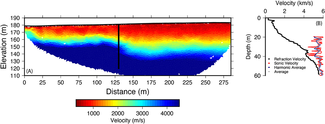
Figure 2. P-wave and sonic velocity results presented by Holbrook et al. (2019). (A) P-wave velocity profile. (B) Comparison of sonic velocity (red) vs. extracted 1D velocity profile from (A). The blue line is the harmonic average ( $\frac{n}{\sum_{i = 1}^{n} \frac{1}{v_{i}}}$ ) and the gray line is the geometric average ( $\frac{\sum_{i = 1}^{n} v_{i}}{n}$ ) every 2 m in depth.

We use a detailed set of borehole and seismic refraction observations in a weathered and fractured granite in the Laramie Range, Wyoming, to show the scales over which seismic refraction data provide valid information about CZ structure. Our observations in the Laramie Range are consistent with those at the South Carolina site (Holbrook et al., 2019), in that they show a distinct discrepancy between sonic (10s of cm scale) and seismic refraction velocities (10s of m scale) in the fractured rock region of the CZ. However, at this site we have another observation, 500 m away in a similar rock type, where the refraction and sonic velocities agree. Here we demonstrate that seismic velocity in the CZ is scale-dependent, and that the discrepancy between sonic and refraction velocities is not an error, but rather information about fracturing. This discrepancy, attributed to the contrasting measurement scales, is observed in other disciplines as well and is similar to measuring hydraulic conductivity on a small core sample and comparing this value to a large-scale pump test, or comparing the geochemical composition of a small piece of core against the composition of cuttings averaged over 10s of meters. We hypothesize that the magnitude of the velocity discrepancy derives from the scale of heterogeneities present in the fractured rock layer of the CZ. Although refraction images are unable to resolve small-scale heterogeneity (10s of cm to a few meters), the resulting structure is still clearly influenced by this heterogeneity. When interpreted in this context, we argue that seismic refraction remains a crucial geophysical tool to characterize the deep CZ structure across landscapes.

Site Description

Our study site is in the Laramie Range, Wyoming, where Sherman granite weathers to a thick grus layer (Eggler et al., 1969; Evanoff, 1990; Frost et al., 1999). The field site sits on gently undulating topography, which has been interpreted to be an ancient weathering surface that was uplifted during the Laramide Orogeny and is still being eroded (Gregory and Chase, 1994; Chapin and Kelley, 1997). Outcrops of Sherman granite exist in the northwest and southwest corners of the study area but are otherwise absent; one notable outcrop is located ~100 m southeast of hole BW-3 (Figure 3). There is no evidence of Quaternary glaciation, but it is likely that the site was much colder than the modern average temperature of 5.4°C. The site receives 620 mm of precipitation annually, most of which is in the form of snow (NRCS, 2021).

FIGURE 3

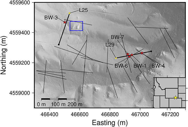
Figure 3. A hill shaded relief map of the study site. The outcrop near BW-3 and L25 is highlighted by a blue box. Red stars indicate the locations of boreholes. The two lines used in this study are thick black lines, where the yellow point indicates the start of the profile. The thin transparent profiles are existing seismic refraction lines presented by Flinchum et al. (2018a,b). The boreholes BW-6, BW-7, BW-1, and BW-4 are all within 70 m of each other.

Over the course of 3 years (2013–2016) 30 seismic refraction profiles, totaling more than 7 km in length, were collected by the Wyoming Center for Hydrology and Geophysics (Flinchum et al., 2018a,b, 2019; Novitsky et al., 2018; Hayes et al., 2019). The deep CZ structure has also been imaged with passive seismic methods (Keifer et al., 2019; Wang et al., 2019a,b). The site contains nine boreholes ranging in depth from 16 to 73 m (Figure 3) (Flinchum et al., 2018a; Ren et al., 2019). Downhole optical televiewer logs and casing depths revealed that intact, unweathered bedrock, defined seismically by velocities >4,000 m/s, lies at depths up to 60 m below the surface (Flinchum et al., 2018b). The bedrock velocity of 4,000 m/s was determined from a seismic refraction survey conducted over a relatively unfractured outcrop nearby (Flinchum et al., 2018b). The soft and friable saprolite above the weathered bedrock interface was sampled through a combination of push coring and seismic refraction analysis and shown to be porous (~34%) and have velocities >1.1–1.2 km/s (Flinchum et al., 2018a, 2019).

Methods

Measuring P-Wave Velocity With Shallow Seismic Refraction and Sonic Logging

P-wave velocities presented in this manuscript were acquired by two methods: shallow seismic refraction (SSR) and sonic logging (SL). Both methods rely on the refraction of elastic energy at elastic boundaries. The elastic properties are dependent on the density and bulk and shear moduli of a given material. Refraction is advantageous because the velocity of a material can be determined simply by the first-arrival time of the seismic energy—the phase and amplitude of the arrival can be ignored.

During a SSR survey, the travel times between a seismic source to an array of geophones are measured and inverted to generate a 2D tomogram of seismic velocity (Woodward, 1992; Sheehan et al., 2005; Gance et al., 2012; Zelt et al., 2013). This type of SSR surveying is a robust method that has been used on crustal scales (Mooney and Brocher, 1987; Korenaga et al., 2000; Hayes et al., 2013), hillslope scales (Whiteley and Eccleston, 2006; McClymont et al., 2012; Thayer et al., 2018; Leone et al., 2020), and over outcrops (Holbrook et al., 2014; Flinchum et al., 2018b). SSR sources utilize a low-frequency (10s of Hz) source that produces relatively large wavelengths (10s−100s of meters). In an SSR survey seismic energy can travel 10s−100s of meters both vertically and laterally before being recorded at a geophone.

SL is less common in the CZ because it requires an uncased, large-diameter (2” or greater) borehole. In addition, sonic logs only work beneath the water table, since water couples the sonic source and receivers to the surrounding rock. Due to these constraints, only a limited number of studies have used sonic velocities to study the top 100 m of Earth's surface (Watson et al., 2005; Martí et al., 2006; Holbrook et al., 2014; Raef et al., 2015; Flinchum et al., 2018a; Gu et al., 2020a). The acquisition of a sonic velocity via SL works on the same principles as the SSR survey; that is, velocity is obtained by measuring the time taken to travel between a source and multiple receivers. In the SL case, however, most of the energy is traveling vertically, at right angles to the majority of travel paths in SSR.

There are a few important differences between the SSR and SL. First, during a SL survey, the maximum offset between the source and receivers will be limited by the tool length, often to 10′s of centimeters to a few meters, in contrast to the 10′s−100's of meters that might separate a source and geophone during SSR. The tool is moved up and down the hole in centimeter increments, providing estimates of velocity every few centimeters. Second, the sonic tool uses a source frequency that is 2–3 orders of magnitude higher than those used in a seismic refraction survey (our study is comparing ~80–15,000 Hz). The higher frequencies produce wavelengths 2–3 orders smaller than refraction. Finally, given that water couples the source and receiver to the borehole wall, the first arrival from energy will be critically refracted along the water/rock interface making it sensitive to a thin region along the borehole wall.

Shallow Seismic Refraction (SSR)

We reprocessed two SSR refraction lines that were part of a larger study presented by Flinchum et al. (2018a,b). L29, which extends from the top of the gently undulating ridge into the valley to the east, intersects boreholes BW-1 and BW-4 and comes within 10 m of holes BW-6 and BW-7 (Figure 3). A sledgehammer source was used by striking a stainless steel plate; hammer swings were stacked at least 8 times to improve the signal-to-noise. L29 was collected with 240 channels at 1 m spacing with shots every 12 m. L25 was collected with 96 channels at 2.5 m spacing with shots every 10 m. On L25, three off-end shots extending 30 m before the first geophone and 30 m past the last geophone were also collected. There were no off-end shots collected on L29.

For the SSR surveys, arrival times were picked manually. To pick the arrivals, shot gathers were trace normalized. We made as many picks as possible on the trace-normalized data without aid of any filtering. After picking on the unfiltered data, we applied a band-pass filter between 10 and 150 Hz to help identify far-offset arrivals. After picking, L29 contained 3935 first arrival picks and L25 contained 2039 picks (Supplementary Figure S1). In cases where the first arrival was noisy or could not be determined, no pick was made, to avoid adding errors into the final models.

To invert the first-arrival times and produce a 2D image of seismic velocities we use the Python Geophysical Inversion Modeling Library (PyGIMLi) (Rücker et al., 2017). PyGIMLi utilizes a shortest path algorithm (Dijkstra, 1959; Moser, 1991; Moser et al., 1992), which models seismic energy propagation as rays, not as waves. The shortest path algorithm is used in many other travel-time tomography codes (e.g., Zelt et al., 2013). The shortest path algorithm calculates a path through the velocity model—referred to as a ray path. The ray paths are used to mask areas in the final velocity that are not constrained by the data. In other words, if a ray path does not pass through a given cell in the model it will not be plotted. Ray paths tend to be curved in appearance because they refract toward the surface when velocity increases with depth. As a result, the resolved depths of the models vary spatially as driven by the data.

PyGIMLi utilizes a deterministic Gauss-Newton inversion scheme (Gance et al., 2012) which requires a data weight for each travel-time pick. These data weights are used to drive the error weight matrix and ultimately influence the final model fits. Here, instead of assigning a constant error value to each pick we used a linear equation as a function of offset (distance from source) line length,

\begin{array}{l} error = \frac{0.003 * offset}{line length} + 0.0005 & (1) \end{array}

where offset is the distance [L] between the source and the geophone. Using Equation 1 means that the errors start at 0.5 ms and increase linearly to a maximum of 3 ms at the spread length. We chose a maximum error of 3 ms because of the high quality of the data. Each associated error is read into the inversion and used to weight the travel-times, such that travel times with the smallest errors are given the most weight.

To compare P-wave velocities derived from SSR with those from SL, it is important to quantify uncertainty on the velocities produced by the tomography. To quantify uncertainty, we randomly resampled the travel-time data, to utilize the large amount of input travel-times and randomly remove influences for each one. To achieve this, both L29 and L25 were inverted 20 times on the same mesh with the same inversion parameters, with 40% of the travel-time picks randomly removed before each inversion. Velocities at each pixel in the mesh were averaged together from all inversion realizations to produce an average 2D velocity model as well-standard deviations expressed as a percentage of velocity (Supplementary Figures S2, S3). We then use the average velocity profile to trace all the picked arrival times, so that the final fitting criteria for the tomograms shown here use all of the first arrival picks. We also compute the vertical velocity gradient (dv/dz) for each averaged tomographic model to highlight vertical changes in velocity.

Sonic Logging (SL)

For the SL acquisition, we used a Mount Sopris 2AFWS (Colorado, USA). The downhole instrument is ~ 3.0 m long with an insulator separating the source from the three receivers. The distance between the source and receivers is fixed at 0.91, 1.22, and 1.52 m. The source has a center frequency of 15 kHz. To process the downhole data, we recorded the elastic wavefield response at each of the three receivers. The elastic wavefield recording allows us to determine P-wave velocities by picking the first arrival times. As the tool travels through the borehole a source is generated at 5 cm intervals. To aid in the picking of arrivals, a semblance plot is created by summing the amplitudes of the waveforms along fifteen different slowness values (1/velocity) using a 50 μs window for every depth sampled. The best-fitting velocity from each source location (every 5 cm) was auto-picked based on the highest semblance value. After the automatic picks were made across the entire borehole depth, the picks are visually inspected, and erroneous picks are manually adjusted or removed. Because water in the borehole is required to couple the seismic source and geophones, sonic velocity logs do not exist for the unsaturated zone near the surface. Our data set consists of P-wave velocity profiles below the casing and below the water table for all five boreholes in this study (Figure 3).

The Relationship Between Velocity and Porosity

In areas with crystalline bedrock, we can assume that the porosity of intact bedrock is near zero, so that changes in the seismic velocity must be due to porosity generated through chemical and physical weathering processes (including fractures). The strong relationship between porosity and velocity has allowed for the estimation of porosity in the CZ from seismic refraction data (Holbrook et al., 2014; Flinchum et al., 2018a; Hayes et al., 2019; Callahan et al., 2020). Several rock physics models link porosity to velocity, including porous media models (Hashin and Shtrikman, 1963; Dvorkin and Nur, 1996; Dvorkin et al., 1999) and differential effective media (DEM) (Budiansky and Oconnell, 1976; Berryman et al., 2002a,b). A DEM model is appropriate when the pore spaces do not form a single connected network (Berryman et al., 2002b), consistent with the conceptual framework of the fractured rock region (Berryman et al., 2002b).

Regardless of which rock physics model is used, an increase in porosity will always result in a decrease in P-wave velocity if lithology and saturation remain constant. The rate of velocity decrease depends on the pore structure and mineralogy. In fractured media models, small increments in porosity can significantly reduce velocity. Following work by Flinchum et al. (2018a), we modelled porosities and velocities measured on granitic rocks around the world using a DEM derived by (Berryman et al., 2002b), which assumes interconnected penny-shaped inclusions throughout the material. We obtain the bulk and shear moduli of the unfractured medium using the Voigt-Reuss-Hill average (Hill, 1963; Mavko et al., 2009). The effective elastic moduli and of the fractured material are then obtained by solving a system of differential equations from (Berryman et al., 2002b) (Supplementary Material S1). Flinchum et al. (2018a) showed that a DEM model with a crack aspect ratio of 0.016 fit porosity and velocity measurements of weathered granites from multiple studies (Figure 4) (Begonha and Braga, 2002; Sousa et al., 2005; Novakova et al., 2012). The porosity-velocity relationship defined previously by Flinchum et al. (2018a) was calculated using a DEM rock physics model with an approximation for the Sherman granite (Table S1) (Flinchum et al., 2018a). The DEM model produces an exponential decrease in seismic velocity with increasing porosity (Figure 4). Based on the model and observed data (Figure 4) a porosity decrease of 0.10 m³/m³ can result in a velocity increase of ~5,000 m/s. As a result, we expect seismic velocity to be highly sensitive to variations in porosity or fracture density in the CZ.

FIGURE 4

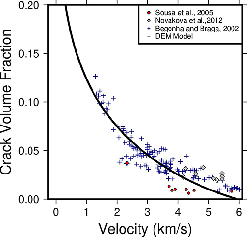
Figure 4. Observed (symbols) and modeled (solid line) porosity and velocity relationships for weathered and fractured granites (Begonha and Braga, 2002; Sousa et al., 2005; Novakova et al., 2012). In this case a small amount of porosity, or crack volume fracture, can significantly reduce the P-wave velocity. The modeled porosity follows the differential effective medium model and mineralogy described by Flinchum et al. (2018a). The equations, parameters, and minerology used to calculate the model are provided in the Supplementary Materials (Section S1).

Results

Heterogeneity

The CZ structure in the weathered and fractured granite at the study site is laterally heterogeneous. A Mount Sopris QL40-OBI-2G Optical Televiewer was deployed to provide a 360° unwrapped optical borehole image (OBI) at each of the boreholes. We converted the images to black and white and boosted the contrast to emphasize fractures and heterogeneity in the rock. The OBI logs and sonic logs based on both seismic velocities from the four deep (> 50 m) boreholes, all located within 70 m of each other, show strong lateral heterogeneity in the fractured rock directly below the casing (Figure 5). Downhole hydraulic conductivity logging revealed that hydraulic conductivity varies over two orders of magnitude but generally decreases with depth (Ren et al., 2019). Other geophysical studies have shown that the influence of heterogeneous remnant fabric from fractures extends upward into the saprolite (Novitsky et al., 2018) and that the depth to the intact bedrock is also laterally heterogeneous on the 100s−1,000s of m scale, extending as deep as 60 m below the surface (Flinchum et al., 2018b; Keifer et al., 2019; Wang et al., 2019a). In addition, nuclear magnetic resonance (NMR) logging was completed at all of the boreholes in the study area and show low but variable water contents (<0.15 m³/m³) in the fractured rock region of the CZ; the water is focused in visibly fractured regions (Flinchum et al., 2019; Ren et al., 2019). The fracture density in the fractured rock layer inferred from NMR is highly heterogeneous, with porosity varying from 0 to 0.15 m³/m³.

FIGURE 5

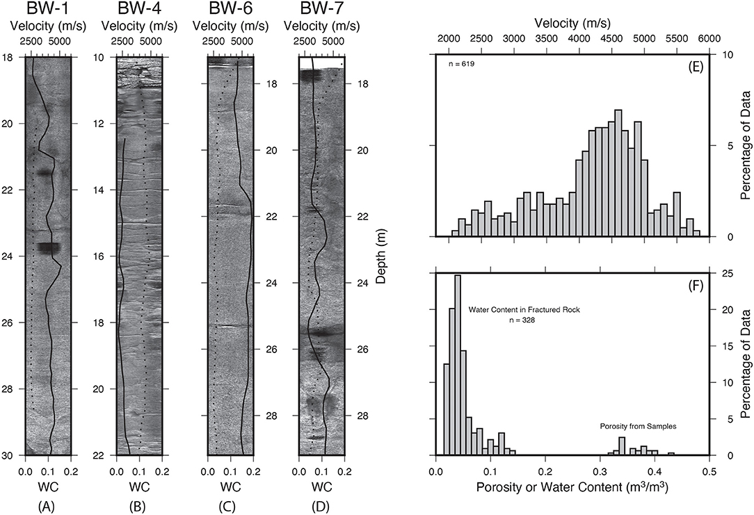
Figure 5. Observations of lateral heterogeneity in the fractured rock of the CZ at the study site. (A–D) Optical televiewer logs from the top 12 meter immediately below casing. The images were converted to black and white, and the contrast was boosted to emphasize the differences in fracture density. The dotted line are the maximum water contents reported by Flinchum et al. (2018a). The solid black line is the P-wave sonic velocity. When the velocity is higher, the water content is lower. (A) BW-1 (B) BW-4 (C) BW-6, and (D) BW-7 (E) Histogram of the P-wave velocities for the sonic logs below casing in BW-1, BW-4, BW-6, and BW-7. It is assumed that all velocities come from the fractured rock region of the CZ. Note that the average value occurs between a value of 4,000–5,000 m/s. Velocities on outcrop in the Laramie Range and Southern Sierras report between 4,000 and 4,500 m/s (Holbrook et al., 2014; Flinchum et al., 2018b). (F) Histogram distribution of water contents below casing (thus the fractured rock region) from reported by Flinchum et al. (2018a). Also included in the histogram are the 25 hand measure porosity from the saprolite reported by Flinchum et al. (2018a). Porosity in the fractured rock region is generally <0.06 m³/m³.

Comparing P-Wave Velocities Derived From SSR and SL

At L29, the SSR profile is generally divided into two domains. The first domain is defined by velocities < ~1,800 m/s (warmer colors in Figure 6A). The second domain is defined by velocities > ~4,000 m/s (cooler colors in Figure 6A). These two domains are separated by a thin transitional region where velocity increases rapidly over a short vertical distance (~5–10 m) with gradients of 100–300 m/s/m (Figure 6B). The vertical velocity gradient image (Figure 6B) highlights this transition or boundary separating these two domains. This boundary is deepest (> 50 m) under the ridge (between 25 and 100 m along the profile) (Figures 6A,B) and comes within 10 m of the surface under the valley (between 210 and 240 m along the profile) (Figures 6A,B). The strong increase in velocity can also be observed in the travel-time picks and represents the most significant seismological boundary revealed by the surface refraction data (Supplementary Figure S1).

FIGURE 6

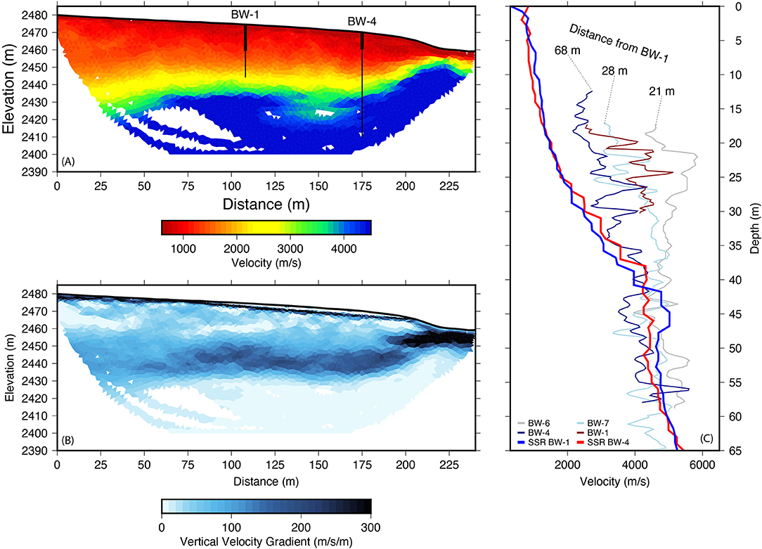
Figure 6. Travel-time tomography results for L29. (A) Final P-wave velocity model estimated by travel-time tomography. Model fits and uncertainty are provided in the supplementary material (Supplementary Figure S2). The models are masked by ray paths. Borehole locations are show as vertical line where the thickest part of the line represents the casing. The bottom of casing is interpreted to indicate the top of fractured bedrock. The profile intersected BW-1 at 108 m and BW-4 at 175 m. BW-6 and BW-7 both occur at 80 m along the profile but do not intersect. BW-6 is ~10 m south of the profile and BW-7 is ~10 m north of the profile. (B) Vertical gradient of velocity calculated at each pixel in the model. Dark colors indicate a sharp increase in velocity vertically and highlight the location of the strong elastic boundary in the model. (C) Comparing the refraction and sonic velocities. In this plot, everything is converted into the depth domain using the topography from the LiDAR (Figure 1). The thin colored lines are sonic velocity profiles from the borehole logs. Logs start at different depths because of different casing depths and variations in the water table. Distances from BW-1 are marked on each profile. The thicker blue and red lines are extracted vertical velocity profiles from panel a from BW-1 and BW-4 locations shown at 108 and 175 m.

Sonic velocity logs from BW1, BW-4, BW-6, and BW-7, which are on or near seismic profile L29 (Figure 3), show significant variability above 40 meters depth (Figure 6C). This variability is surprising, given that BW-4, BW-6, and BW-7 lie within 30 m of each other and BW-1 is only 70 m from BW-4 (Figure 3). Between 20 and 25 meters depth, for example, the velocity at BW-4 is ~3,000 m/s, while at BW-6 it is ~5,000 m/s. This variability disappears below about 40 m depth, where the sonic velocities converge to a velocity of ~4,500 m/s (Figure 6C).

Extracted 1D velocity profiles from the surface refraction data are smooth and lack both the detailed vertical structure and the lateral heterogeneity that is observed in the sonic velocities (Figure 6C). Above 40 m depth, where strong variability in sonic velocities occurs, refraction velocities are slower by as much as 4,000 m/s (Figure 6C). Despite the large differences in the shallow parts of the borehole, the tomographic velocity and sonic velocities converge to a common velocity between 4,000 and 5,000 m/s (Figure 6C), close to the 4,000–4,500 m/s measured by surface refraction on granite outcrops in the Southern Sierras (Holbrook et al., 2014) and nearby in the Laramie Range (Flinchum et al., 2018b). The discrepancy between the sonic velocities and travel-time velocities above 40 m is not a processing or inversion artifact (Figure 6C). We conducted a forward model study using the sonic velocities to predict SSR travel times for L29. The forward modeling results show clearly that the sonic velocities are too fast to explain the observed travel times (see Supplementary Materials S2, S3). Furthermore, similar discrepancies have been observed in the Piedmont of South Carolina (Figure 2) (Holbrook et al., 2019) and at a minimum of three other sites worldwide (Watson et al., 2005; Martí et al., 2006; Raef et al., 2015).

Just 500 m northwest of profile L29, the sonic and refraction velocities on line L25 show a much better match at all depths with overlapping observations (Figure 7). As with L29, the SSR profile can be divided into two domains: one with velocities < ~1,800 m/s, and one with velocities > ~4,000 m/s (Figure 7A). In this second refraction profile (Figure 7A), the seismic refraction velocity shows a high velocity zone that comes to the surface and extends 100s of meters laterally (Figure 7A).

FIGURE 7

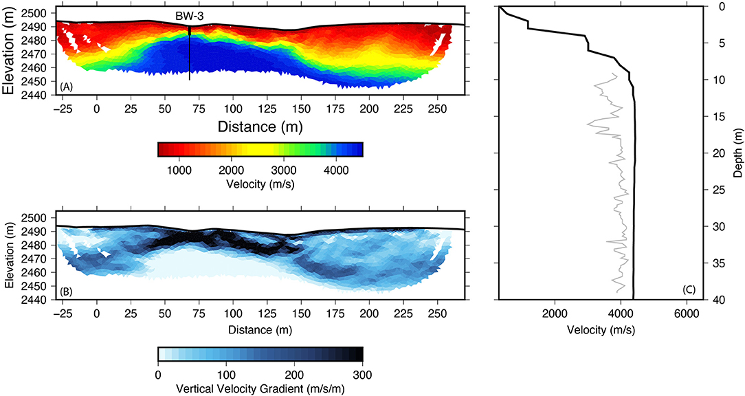
Figure 7. Travel-time tomography results for L25. (A) Final P-wave velocity model estimated by travel-time tomography. Model fits and uncertainty are provided in the supplementary material (Supplementary Figure S3). The models are masked by ray paths. The borehole location is show as vertical line where the thickest part of the line represents the casing. The profile intersected BW-3 at 68 m. (B) Vertical gradient of velocity calculated at each pixel in the model. Dark colors indicate a sharp increase in velocity vertically and highlight the location of the strong elastic boundary in the model. (C) Comparing the refraction and sonic velocities. In this plot everything has been converted into the depth domain using the topography from the LiDAR (Figure 1). The thin colored gray line is the sonic velocity profile from the borehole log. The thick black line is the extracted vertical velocity profile from panel “a” and the thin gray line is the sonic velocity profile from BW-3.

The L25 profile crossed a depression in the landscape, so the water table is at ~7 m depth. This shallow water table allowed us to acquire sonic velocities closer to the surface than in any of the other boreholes (Figure 3). At this location, the sonic velocities and the seismic refraction velocities are in much better agreement (Figure 7C). The match is not perfect, however: the SSR velocity at L25 is about ~10% higher (~4,300 compared to ~3,900 m/s) than the sonic velocities observed in the borehole (Figure 7C). This is most likely caused by the strong vertical velocity gradient near the surface, which is a difficult structure for travel-time tomography to resolve. This area of the model has our highest uncertainty estimates (Supplementary Figure S3e). The uncertainty in the strong vertical velocity gradient near the surface would have the tendency to make the velocities near the surface slightly slower and the velocities at depth slightly faster to fit the observed travel times. Thus, we believe that the 1D velocities at L25 (Figure 7C) agree within error. Additionally, the surface refraction velocity profile still lacks the velocity detail observed in the sonic profile, and both velocities converge to an average velocity of ~4,000–4,500 m/s, consistent with velocities collected over outcrop in the Southern Sierras (Holbrook et al., 2014) and the Laramie Range (Flinchum et al., 2018b).

Discussion

The Seismic/Sonic Velocity Discrepancy

One of the challenges of studying CZ processes is integrating a wide variety of observational data across different spatial scales (e.g., mineralogical vs. hillslope vs. landscape scales). The discrepancy between refraction and sonic velocities (Figures 2B, 6C) might appear to beg an obvious question: which velocity is “correct”? Here we argue that the answer is that both velocities are correct, at the wavelengths over which they are measured. Neither velocity is in error; rather, the velocities differ because they sense fracture densities that are scale-dependent. Before presenting our argument, we must first address whether the observed sonic/refraction velocity discrepancy is due to vertical anisotropy. Anisotropy is the ratio between seismic velocities measured in different directions. In general, seismic velocities travel slower across foliation or fractures (Novitsky et al., 2018; Eppinger et al., 2021). The seismic waves produced by SSR travel largely in the horizontal direction, whereas the seismic waves produced by SL largely travel in the vertical direction, raising the idea that pervasive, near-vertical fractures would cause slower refraction velocities than sonic velocities. However, vertical anisotropy cannot explain the velocity discrepancy we observe for several reasons. First, the anisotropy values required to explain the SSR/SL discrepancy would need to be as high as ~100%, which is far higher than observed anisotropy due to fracturing elsewhere (e.g., Crampin et al., 1980; Maultzsch et al., 2003). Second, faster velocities in the vertical direction would imply pervasive near-vertical fracturing. While fracturing exists at our site, the amount of anisotropy observed in the saprolite (Novitsky et al., 2018) is modest (maximum 12%), and we are unaware of processes that would explain 100% anisotropy in the fractured bedrock with only ~10% anisotropy in the saprolite. Third, numerous near-horizontal fractures are observed in the borehole optical logs (Figures 5A–D)—a pattern that should create faster velocities in the horizontal direction. Finally, decreases in sonic velocity between the boreholes at Blair correlate strongly with fracture density observed in the boreholes (Figures 5A–D). This suggests that sonic velocities are controlled by the number of fractures in a given volume (i.e., fracture density), not the orientation of the fractures.

In the case of our sonic and seismic waves passing through the fractured bedrock layer, the wavelengths differ by two orders of magnitude (v = fλ): a seismic P-wave with a dominant frequency of 40 Hz traveling at 2,000 m/s would have a dominant wavelength of 50 m, while a sonic P-wave at 6 kHz and 3,000 m/s has a wavelength of 50 cm (Figure 8). P-waves propagate by compressing and dilating the material at the scale of the seismic wavelength. This, in turn, means that the seismic wave senses all the fractures present in a volume ~50 m in diameter, while the sonic wave only senses fractures within a 0.5 m diameter. The volume that is deformed by this compression is related to the wavelength and is known as the representative elementary volume. The volume can change with scale depending on the heterogeneity of the material. The representative elementary volume is an important concept that can used to explain the variation of a physical property with upscaling (Matonti et al., 2015; Bailly et al., 2019).

FIGURE 8

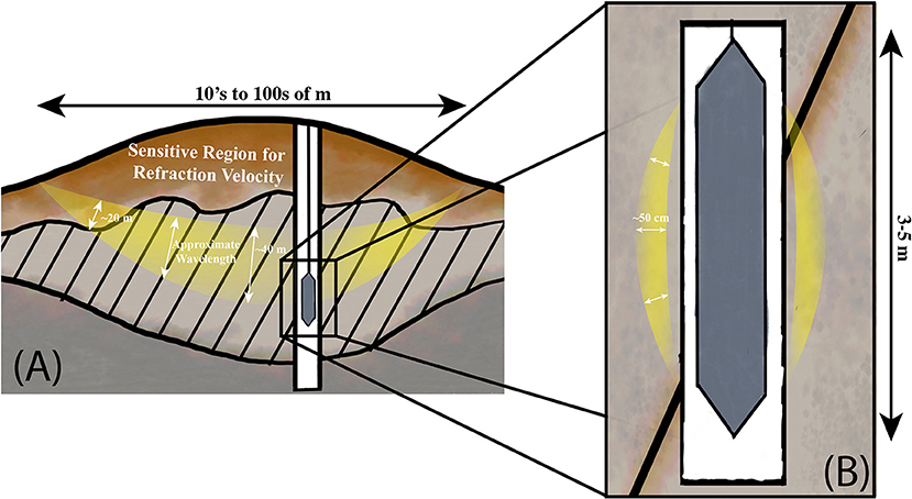
Figure 8. A conceptual model illustrating the contrast in scales between a large-wavelength seismic wave (A) and a small-wavelength sonic tool (B). Diagonal lines represent parallel fractures in the fractured bedrock layer. A seismic wave traveling from the source (star) to receiver (triangle) may have a wavelength of ~50 m in the fractured bedrock layer However the wavelength changes as a function of velocity (Supplementary Figure S6). As a result, the wave “feels” a pervasively fractured medium and propagates at a correspondingly low velocity (say, 2,000 m/s). The sonic tool, in contrast, may have a wavelength of ~0.5 m, such that it senses fully intact, high-velocity bedrock in between fractures, and lower velocities as it crosses individual fractures. As a result, the refraction velocity will be substantially lower than sonic velocities in a fractured medium.

To use a hydrogeology analogy, we postulate that comparing sonic and refraction velocities is similar to comparing hydraulic conductivity measurements of a fractured aquifer obtained with a pump (i.e., transmissivity) test with measurements made in the lab on a small sample. Apparent hydraulic conductivity is well-known to scale with the measurement, where small scale measuremetns tend to show lower hydraulic conducitvites (Neuman, 1988; Clauser, 1992; Rovey and Cherkauer, 1995; Schulze-Makuch and Cherkauer, 1998). In most cases, depending on how the sample was obtained, the lab sample will have a lower hydraulic conductivity because the pump test is an average of high and low hydraulic conductivity fractures along the entire length of the borehole (Clauser, 1992) (equivalent to the large yellow area in Figure 8). It is not uncommon in fractured rock aquifers to have one or two highly productive fractures while others do not contribute to flow (Sausse and Genter, 2005; Lee and Kim, 2015).

The analogy of hydraulic conductivity is useful but imperfect, in one respect: in the case of hydraulic conductivity, the length of the screened area or the location of the sample are known, while in the case of seismic refraction, the wavefield is complex (Supplementary Figure S5), and wavelength varies as a function of velocity and source frequency (Supplementary Figures S4, S5). The velocity is affected by the porosity distribution of the CZ, which is, by definition, site specific. (Liu et al., 1976; Xia et al., 2003; Tisato and Marelli, 2013). Fluid in pore space can cause frequency dependent attenuation in the form of Wave Induced Fluid Flow (WIFF) (Müller et al., 2010). In seismic refraction, the elastic energy can travel 100s of meters from source to receiver (Figure 8). The combination of these physical phenomena makes it difficult to explicitly define the sample region represented by the travel-time observation.

We hypothesize that velocities measured across such vastly different scales in a porous medium would only be equal if the fraction of pore space was equal across those scales—essentially, if the distribution of pore space is uniform. Refraction and sonic velocities would match if we collected a seismic refraction profile over a borehole with sonic velocities in a location where the underlying rock has a homogenous porosity distribution—that is, if porosity is equal regardless of the sample volume. While such a fairly uniform distribution of porosity can occur in a sedimentary rock (e.g., a clean sandstone or a gravel aquifer), it is unlikely to be true when porosity is due to fractures. Fractured materials can have highly non-uniform fracture distributions across a wide variety of scales. We illustrate this point with a simple example: a layer of bedrock pervasively broken by evenly spaced fractures (Figure 8).

If fractures are 1 m apart and each have an aperture of 4 cm, then within the 50-m wavelength of a seismic P-wave, there will be 50 × 0.04 = 2 m of open fracture space, or a fracture porosity of 4% (2/50). Given the strong sensitivity of P-velocities to fracture porosity, adding 4% porosity to the bedrock could easily reduce seismic velocities from, say, 4,500–2,000 m/s (Figure 4). The seismic wave travels at this relatively slow velocity throughout the fractured bedrock layer, and its travel times in the refraction data reflect that slow propagation. The sonic tool, in contrast, with its wavelength of around 50 cm, would measure non-weathered and unfractured rock (velocity 4,000–4,500 m/s) except when crossing an individual fracture (Figure 8), when the velocity would drop precipitously—exactly as observed in the sonic logs of Figures 6B, 7B.

For this reason, we hypothesize that the persistent discrepancy between seismic and sonic velocities in the fractured bedrock layer of the CZ in South Carolina (Holbrook et al., 2019) (Figure 2) and the Laramie Range (Figure 6) should be viewed not as an error, but rather as valuable information. Seismic velocities that consistently underestimate sonic velocities are a sign of pervasive fracturing at scales between the respective seismic and sonic wavelengths. Where the two velocities agree, in contrast, then porosity is likely uniformly distributed. This is the case in Figures 2, 6B at depths >40 m, where the relatively high velocities suggest that the meter-scale fractures are largely closed due to ambient pressure (e.g., St. Clair et al., 2015).

What Do P-Wave Velocities Tell Us About CZ Structure?

Under our proposed hypothesis, velocity models produced by seismic refraction tomography will be blind to small-scale (10s of meters) heterogeneity but will still be able to quantify the thickness of the CZ across landscapes over 100s of m. Seismic refraction still remains a particularly powerful geophysical tool to explore the deeper regions of the CZ, especially if the CZ boundaries of interest are controlled by changes in porosity or fracture density. The velocity profiles derived from seismic refraction represent large-scale averages that reflect the dominant seismic wavelength. It remains difficult to quantify the volume that this average represents, since quantifying the volumes would require a fully 3D seismic waveform solution. Full waveform inversions, even in 2D, are still in their infancy when working in the strong velocity gradients associated with near-surface materials (Gao et al., 2006, 2007; Virieux and Operto, 2009; Romdhane et al., 2011).

Despite the lack of sensitivity to small-scale structures, seismic refraction remains one of the only geophysical tools that can quantify the general location of boundaries defined by changes in porosity in the CZ over landscape to watershed scales. The seismic refraction method suffers from the classic tradeoff between velocity detail and spatial coverage, and users need to be aware of the relevant wavelength scales to interpret the images correctly. Although high-frequency sonic velocity logs in the CZ remain rare, our data show that P-wave seismic velocity is scale-dependent. Given the interdisciplinary nature of CZ science, it is likely that the 2D profiles of velocity will be used to inform or test conceptual models of CZ evolution (West et al., 2019; Leone et al., 2020). It is important to realize that the velocities in seismic refraction tomography represent large-scale averages over the scale of their dominant wavelength. While smaller-scale heterogeneity certainly exists beneath the lateral and vertical resolution of the refraction inversion, the velocity discrepancy itself is not a consequence of the inversion, but rather of the physics of wave propagation at different wavelengths. Understanding this large-scale averaging is particularly important at sites where velocities are used quantitatively to estimate porosity (Mota and Santos, 2010; Flinchum et al., 2018a; Callahan et al., 2020; Gu et al., 2020b) or strain (Hayes et al., 2019).

Our results show that the refraction and sonic velocities converge at depths where the fracture density is uniform, consistent with the idea of a protolith that is defined by a small, uniform porosity. The sample volume is not straightforward, as wave propagation physics is complicated, but a good rule of thumb is that the wavelengths, which depend on the velocity and frequency content of the source, provide a rough estimate of the averaging scale that the velocities represent.

Conclusions

P-wave velocities estimated from surface refraction tell us about the CZ structure on scales of 10s−100s of m. Sonic velocities are more sensitive to fracture density and CZ heterogeneity. The velocity profiles generated by seismic refraction tomography are blind to small-scale (< 10 m) heterogeneity but successfully image the thickness of the CZ across landscapes. The lack of sensitivity to smaller-scale structures means that refraction velocities must be interpreted in the context of their wavelengths, as they will not be able to determine if a boundary is sharp, gradational, or laterally heterogeneous. Despite the lack of sensitivity to smaller-scale structures, surface seismic velocity remains one of the most useful physical properties for detecting the bulk transitions from weathered to less weathered bedrock.

There is still much to learn from seismic velocities of CZ structure. There still exists a spatial gap between the cm scale (sonic velocities) and 10s−100s of m scale (seismic refraction). The lack of high-frequency velocity measurements on samples, either by sonic logs or laboratory tests, leaves a significant gap in our understanding of the scalability of seismic velocities in the CZ. Our work shows that mismatches between sonic and refraction velocities are properly viewed not as artifacts or errors, but rather as information about the spacing and density of fractures.

Data Availability Statement

The original contributions presented in the study are included in the article/Supplementary Material, further inquiries can be directed to the corresponding author. Geophysical data used in this article is hosted on Hydroshare and can be downloaded here: http://www.hydroshare.org/resource/5c6dd575e27f44159f826e4c1c20bf19 (Flinchum, 2021).

Author Contributions

All authors have been actively involved in data collection, processing, and development of ideas presented in this manuscript.

Funding

This work was supported by NSF (EPS-1208909, 1531313, and EAR- 2012353).

Conflict of Interest

The authors declare that the research was conducted in the absence of any commercial or financial relationships that could be construed as a potential conflict of interest.

Publisher's Note

All claims expressed in this article are solely those of the authors and do not necessarily represent those of their affiliated organizations, or those of the publisher, the editors and the reviewers. Any product that may be evaluated in this article, or claim that may be made by its manufacturer, is not guaranteed or endorsed by the publisher.

Acknowledgments

We are grateful to many others for thoughtful discussions and constructive criticism to improve the manuscript. We are also grateful for Dr. Ty Ferre for very insightful comments during review of this manuscript.

Supplementary Material

The Supplementary Material for this article can be found online at: https://www.frontiersin.org/articles/10.3389/frwa.2021.772185/full#supplementary-material

References

Anderson, S. P., Blanckenburg, F., von, and White, A. F. (2007). Physical and chemical controls on the critical zone. Elements 3, 315–319. doi: 10.2113/gselements.3.5.315