 William J. Baule
 Jeffrey A. Andresen1,2
 Julie A. Winkler
- 1Department of Geography, Environment, and Spatial Sciences, Michigan State University, East Lansing, MI, United States
- 2Great Lakes Integrated Sciences + Assessments, School for Environment and Sustainability, University of Michigan, Ann Arbor, MI, United States
Changes in precipitation can have broad and significant societal impacts. A number of previous studies that analyzed changes in precipitation across the Great Lakes and Midwest for a variety of time periods and using a range of quality-control standards and methods observed increased precipitation rates and totals, although there was considerable site-to-site variability, even for sites in close physical proximity. Biases and discontinuities in precipitation observations may contribute to this variability. This study identifies and examines changes in precipitation utilizing a unique approach to observation series screening over a region encompassing the Great Lakes and broader Midwestern region of the United States for the period 1951–2019. A multiple tier procedure was utilized to identify high quality input data series from the Global Historical Climatology Network-Daily dataset. Annual and seasonal time series of precipitation indicators were calculated and subjected to breakpoint analysis as further quality control. Trends were analyzed across a broad range of related indicators, from totals and frequencies of threshold events to event duration and potential linkages with total precipitable water. Results indicate that annual precipitation has generally increased across the region in terms of totals, although there is substantial variation across the study domain in the significance and magnitude of annual trends by indicator. Annual trends were spatially most consistent across eastern areas of the study domain while relatively greater station-to-station variability in trend significance and magnitude was observed across northern and western portions. Significant trends were generally fewer in number for seasonal precipitation indicators and less spatially coherent. The greatest number of significant trends occurred in fall with the fewest in spring. Correlation of indicator trends with trends of mean total precipitable water suggests weak correlations annually and moderate correlations at the seasonal scale. The trends of the precipitation indicators in our study exhibited more coherent spatial patterns when compared with studies with different quality control criteria, illustrating the importance of quality control of observations in climatic studies and highlighting the complexity of the changing character of precipitation.
Introduction
Precipitation is the longest observed and most widely reported meteorological variable and is an essential component of the Earth's hydrologic cycle (Legates and Willmott, 1990). Precipitation is commonly defined as “the amount, usually expressed in millimeters or inches of liquid water depth, of the water substance that has fallen at a given point over a specified period of time” (Huschke, 1959, p. 438). Although precipitation accumulation at daily, monthly, seasonal and annual scales has received the most attention in the climatological literature (e.g., Contractor et al., 2021), other precipitation characteristics such as frequency, intensity, and duration are as much, if not more, of a concern for many natural and human systems (Trenberth et al., 2003; Bartels et al., 2020). Moreover, changes in one or more precipitation characteristics can have substantial societal implications impacting many sectors, including, among others, agriculture (e.g., Pielke and Downton, 2000; Rosenzweig et al., 2002; Hunt et al., 2020; Kiefer et al., 2021), transportation (e.g., Attavanich et al., 2013; Talukder and Hipel, 2020), and tourism (e.g., Chin et al., 2018).
Changes in precipitation characteristics are a particular concern for the Midwest and Great Lakes region of the United States given the region's unique hydrology (Gronewold et al., 2021) and its agricultural importance and contribution to regional, national and global food security (Angel et al., 2018; Takle and Gutowski, 2020). Not surprisingly, a number of studies have investigated temporal trends in precipitation characteristics either specifically for the region (e.g., Zhang and Villarini, 2019) or as part of larger analyses of precipitation trends in the United States (e.g., Kunkel et al., 2020a). For the most part, these analyses have focused on trends in annual and seasonal precipitation totals (e.g., Schoof et al., 2010), extreme precipitation (e.g., Pryor et al., 2009; Walsh et al., 2014), and/or the frequency of wet days (e.g., Roque-Malo and Kumar, 2017; Bartels et al., 2020). In general, precipitation frequency and total accumulation appear to have increased across the region over the last several decades (Higgins et al., 2007; Dai et al., 2016; Contractor et al., 2021). In addition, the amount of precipitation falling during the heaviest events has increased at a greater rate in the Midwest and Great Lakes region compared to the national average (Angel et al., 2018). Extended dry periods have become less frequent, but their intensity (i.e., length) has increased slightly in recent decades (Groisman and Knight, 2008).
One constraint to comprehensive and accurate analysis of temporal trends in precipitation characteristics at the regional scale is the availability and quality of precipitation observations (Costa and Soares, 2009). Although numerous authors have examined the homogeneity of time series for various climatic variables including daily precipitation (Winkler, 2004; Daly et al., 2007; Wang et al., 2010), many studies employing in-situ climate observations fail to take data quality, other than data completeness, into account, even though the magnitude and sign of temporal trends can be biased by changes in technology, station siting, observing practices and other inhomogeneities that are not necessarily captured by station record completeness or recorded in standard metadata archives (Wang et al., 2010; Williams et al., 2012; Baule and Shulski, 2014). Recent progress in the development of spatial and temporal interpolation schemes and gridded datasets, the integration of radar and satellite derived precipitation estimates with in-situ observations, the development of atmospheric reanalysis products, and the availability of simulations from regional and global climate models have only partially alleviated concerns about data quality (Zhang et al., 2011). The limited periods of record for radar and satellite precipitation estimates constrain their use for estimating temporal trends, and gridded datasets can inherit the inhomogeneities of the underlying station observations, with developers of these datasets often advising against their use for time series analysis (e.g., Daly et al., 2010). Consequently, station-based climatologies, in spite of their limitations, remain the benchmark for the assessment of long-term trends (Kiefer et al., 2021), although caution in their application is critical to guard against misinterpreting temporal trends. Earlier studies of precipitation trends for the Midwest and Great Lakes region frequently used station-level daily precipitation observations from the Global Historical Climatology Network-Daily (GHCN-D) database (Menne et al., 2012) for trend estimation (e.g., Villarini et al., 2011; Janssen et al., 2014; Guilbert et al., 2015; Wu, 2015; Hoerling et al., 2016; Huang et al., 2017, 2018; Roque-Malo and Kumar, 2017; Kunkel et al., 2020a,b). For the most part, quality-control procedures have been limited to those applied by the GHCN-D dataset developers to identify and/or correct for errors and inhomogeneities in the precipitation data (Durre et al., 2008, 2010), supplemented by an evaluation of data completeness (e.g., Kunkel et al., 2020b).
Other studies have investigated the synoptic-scale drivers of precipitation, particularly those associated with extreme precipitation, finding that extreme precipitation events across the Midwest and Great Lakes region are often associated with a westward expansion and strengthening of subtropical high pressure across the western Atlantic Basin (Gutowski et al., 2008) as well as the advection of low-level moisture from the Gulf of Mexico ahead of slow moving tropospheric waves (Winkler, 1988; Zhang and Villarini, 2019), with the latter being more prevalent in the western portions of the region and the former in the eastern areas (Bell and Janowiak, 1995; Konrad, 2001; Weaver and Nigam, 2008). Consistent with these findings, Kunkel et al. (2020a) showed that extreme daily precipitation events across the contiguous United States, including the Midwest and Great Lakes region, are directly related to total precipitable water. Specifically, Kunkel et al. (2020b) examined the relationship between regional trends in total precipitable water and regional trends in extreme precipitation as calculated from GHCN-D station-level time series. These large-scale drivers of precipitation are often amplified or suppressed by regional and local climate drivers such as topography, water bodies, and land use/land cover (Myhre et al., 2016; Kunkel et al., 2020a), which can introduce considerable spatial variability in the temporal trends of precipitation characteristics, especially in the Midwest and Great Lakes region with its large water bodies and varied land use/land cover. For the most part, quality control of the precipitation observations employed in these studies of the synoptic, regional and local drivers of precipitation and their contribution to temporal trends in precipitation was confined to an assessment of data completeness of the precipitation time series.
This study provides a comprehensive assessment of the temporal trends in precipitation characteristics for the Midwest and Great Lakes region that focuses on the quality of available precipitation time series. We employ a three-step quality-control procedure that evaluates the GHCN-D precipitation time series for data completeness, possible observer bias, and potential breakpoints (i.e., discontinuities) with the goal of identifying those GHCN-D stations in which we have the greatest confidence for precipitation trend analysis, thereby increasing confidence in the sign, magnitude, significance, and spatial coherence of precipitation trends. We include a range of precipitation indicators that capture the frequency and persistence of high frequency, low magnitude and low frequency, high magnitude events. Furthermore, we examine the associations between temporal trends in the quality-controlled suite of precipitation indicators and trends in atmospheric moisture. The study findings provide the region's many stakeholders with needed information on long-term trends in precipitation characteristics of concern to them, greater certainty in incorporating these data in planning processes and a high-quality baseline for assessing future trends.
Methods
Study Region and Precipitation Data
For this study, the Midwest and Great Lakes region was defined as the states of Pennsylvania, Ohio, Indiana, Michigan, Illinois, Wisconsin, Minnesota, Iowa, Missouri, Kansas, Nebraska, South Dakota, New York, and North Dakota (Figure 1).

Figure 1. Study region and the United States Historical Climate Network (USHCN) stations (green circles) within the study region that passed the quality control checks for data completeness and lack of observer bias as outlined in the methods. Stations that passed the data completeness check but failed at least one of the tests for lack of observer bias are shown as pink circles. The number of stations that passed the third quality control test (no breakpoints) is given in Table 2.
We analyzed a subset of individual site climate series from the National Centers for Environmental Information's (NCEI) GHCN-D collection (Menne et al., 2012). As a first step in selecting stations for the analysis, we examined the GHCN-D database for station series included in the United State Historical Climatology Network (USHCN; Easterling, 2002) which had at least 90% data completeness for daily precipitation during 1951-2019. Only USHCN sites were considered, as these stations were preselected by NCEI based on record length, data completeness, and historical stability (Menne et al., 2012). Data flagged by the GHCN-D quality control procedures as suspicious were marked as missing (Menne et al., 2012). The length of the study period allowed for trends in the second half of the 20th century and the early 21st century to be assessed while maintaining a relatively large pool of potential stations and reasonable spatial coverage. This first data quality control step led to an initial subset of 317 stations over the study region.
The next quality control step involved using tests proposed by Daly et al. (2007) to check for observer bias in precipitation time series, specifically the underreporting of light (1.26 mm) precipitation amounts and the over-reporting of precipitation amounts evenly divisible by 5 and/or 10 when expressed as inches. As these tests were designed for data originally measured in inches, they are described here using inches (in.) in place of millimeters. The under-reporting check consisted of calculating the ratio of counts between 0.06–0.10 in. (C6−10) and 0.01–0.05 in. (C1−5) as follows:
where C6−10 is the total observation count in the 0.06–0.10-in. range, and C1−5 is the total observation count in the 0.01–0.05-in. range. If the ratio, RL, between C6−10 and C1−5 exceeded 0.60, the station failed the check (Daly et al., 2007).
The tests for errant reporting of values divisible by 5 or 10 were conducted by binning precipitation into 0.01 in. bins, fitting a gamma distribution to the data between 0.03 and 1.00 in., and comparing the predicted (P) and observed (O) frequency of the binned observations with the residual (R) calculated as:
The test for biases in amounts divisible by 5 and amounts only divisible by 10 were carried out separately. For the divisible by 5 test, the first residual mean was calculated by averaging the residuals over all amounts except those divisible by 5 (R1) and the second residual (R5) consisted of the mean of residuals for only amounts divisible by 5 as follows:
where n1 and n5 are the number of ones and fives bins and R1 and R5 are residuals calculated from equation 2. The means for the divisible by 10 bias were calculated similarly, instead using values only divisible by 10. The means were compared using a two-tailed t-test with an alpha level of 0.01.
Examples of output from the second quality control procedures are shown in Figure 2 for two locations, Manhattan, KS HCN which passed all the bias tests at p ≤ 0.01 or RL ≤ 0.6 despite showing a small divisible by 10 bias, and Lamar 7N, MO HCN which failed the bias tests showing a strong under reporting bias, a strong divisible by 5 bias, and a strong divisible by 10 bias. Stations that failed any of the tests were removed from the analysis, leaving a subset of 114 long-term climate series across the Midwest and Great Lakes region for the period from 1951 to 2019 for precipitation indicators.
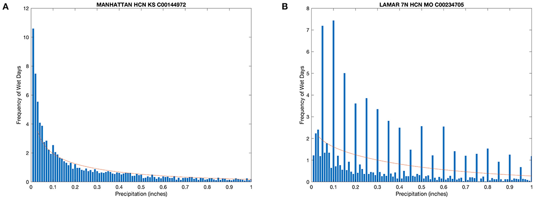
Figure 2. Histograms from two example stations in the study region showing precipitation frequency (blue bars) over the period from 1951 to 2019 binned in 0.01 increments and a gamma distribution (red line) fit to the data following Daly et al. (2007). (A) Manhattan, KS HCN passes (p ≤ 0.01) the tests for underreporting of daily precipitation amounts <0.05 in. (1.26 mm) and for over-reporting of daily precipitation amounts (in inches) evenly divisible by 5 or 10 despite showing a small divisible by 10 bias. (B) Lamar 7N, MO HCN fails all three tests (p ≤ 0.01), showing a strong under reporting bias, a strong divisible by 5 bias, and a strong divisible by 10 bias.
The third quality control step involved checking the time series of the precipitation indicators for breakpoints. Possible sources of discontinuities in the time series include, among others, instrument changes, station moves, and changes in observation protocols including time of observation (Winkler, 2004). Following Mallakpour and Villarini (2016), the Pettitt test (Pettitt, 1979) was applied to identify years when a breakpoint is likely, indicating a non-homogenous time series. A breakpoint was considered significant at p ≤ 0.01, and the time series for that station was excluded from further analysis. This resulted in a variable number of stations per indicator, with the number of excluded stations ranging from none to a maximum of 17. The description of the Pettitt test, following Jaiswal et al. (2015) is: a method that detects a significant change in the mean of a time series, where the exact time of the change (i.e., breakpoint) is unknown, According to the Pettit test, if x1,x2,x3,…xn is a series of observed data which has a break point at t so that x1,x2,x3,…xt has a distribution [F1(x)] which is different from the distribution [F2(x)] of the second part of the series xt+1,xt+2,xt+3,…xn. The non-parametric test statistic is described as follows:
The test statistic K and the associated confidence level (ρ) for the sample length (n) is described as:
When ρ is smaller than the specified confidence level (p), a breakpoint is considered significant.
Precipitation Indicators
This study included a range of precipitation indicators. Several indicators were used to characterize the frequency of non-extreme precipitation, including the number of days with measurable precipitation (e.g., Pryor et al., 2009) and the probabilities of wet-wet day and dry-dry day sequences (e.g., Ines et al., 2011). A wet day was defined as a precipitation total ≥ 1.26 mm (0.05 in) (Groisman et al., 1999). Extreme precipitation was represented in the analysis by indices developed by the Expert Team on Climate Change Detection and Indices (ETCCDI) (Donat et al., 2013) and annual values were calculated using the software packages provided by the ETCCDI Working Group (available at http://www.climdex.org). The extreme precipitation indicators include 10 wet indices and 1 dry index that can be further grouped into percentile-based indices (2), threshold indices (3), absolute value indices (2), duration indices (2), annual accumulation, and “simple” intensity (annual total precipitation divided by the number of wet days). For the percentile-based indices, the base period for defining the percentile value was the 30-year climate normal period of 1981–2010. Descriptions of each of the non-extreme and extreme precipitation indicators are provided in Table 1.
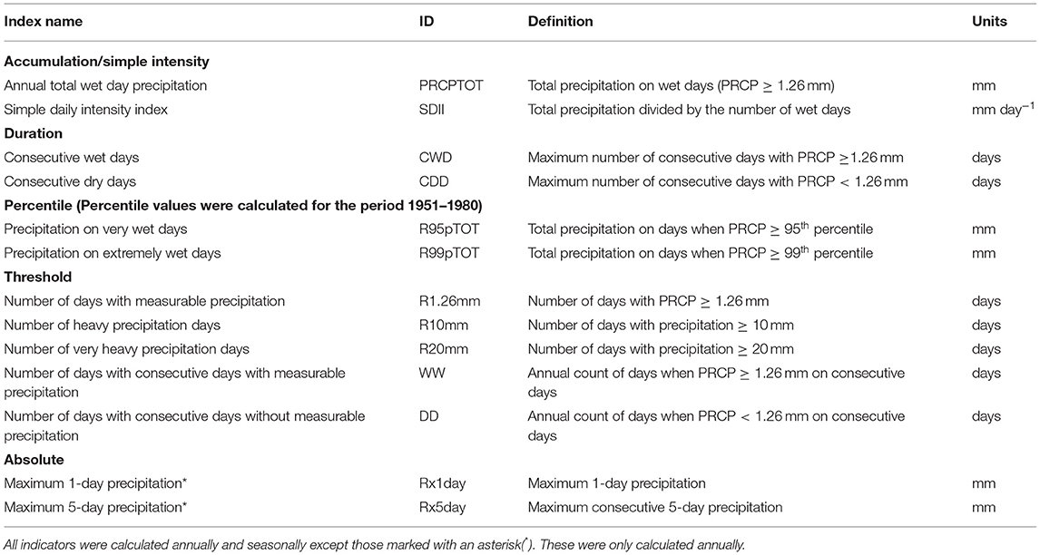
Table 1. Precipitation indicators included in the analysis.
All precipitation indicators were also defined for the climatological seasons of spring (MAM), summer (JJA), fall (SON), and winter (DJF). This is in contrast to most previous studies where precipitation indicators were calculated for annual time steps, with less attention paid to the seasonal variations in the precipitation indicators beyond the frequency of high intensity daily precipitation events (e.g., Mallakpour and Villarini, 2017). Given the importance of precipitation timing and sequencing for numerous regional applications, such as soil moisture and nitrogen movement in agricultural systems (Riha et al., 1996; Bowles et al., 2018) and plant disease risk (Komoto et al., 2021), this study extended the precipitation indicators to the seasonal time step. Additionally, the seasonal analyses provides greater context to more clearly interpret annual trends.
Following the lead of numerous recent studies (e.g., Alexander et al., 2006; Pryor et al., 2009; Shulski et al., 2015; Dai et al., 2016; Roque-Malo and Kumar, 2017), non-parametric statistical methods were employed to estimate the significance and magnitude of temporal trends in the precipitation indicators at the study locations. While a number of potential non-parametric methods were available (e.g., Sneyers, 1990; Sen, 2015; Onyutha, 2021), we chose the two-tailed Mann-Kendall trend test (Mann, 1945; Kendall, 1955, 1975) to test for the significance of potential temporal trends due to its prevalence in previously mentioned studies across the region to allow for intercomparison of results. A strength of the Mann-Kendall method is its ability to assess the significance of trends that are monotonic but not necessarily linear in character. For those locations with significant trends as identified by the Mann-Kendall test, the non-parametric Kendall's tau-based slope estimator (Sen, 1968) was used to obtain a numerical estimate of the temporal trend. All analyses were conducted using three significance levels (p ≤ 0.05, p ≤ 0.10, and p ≤ 0.20) to examine how significance level affects the number of significant trends and their spatial representation. The equations describing the Mann-Kendall test are as follows:
where n is the total length of data, xi and xj are two generic sequential data values, and the following function assumes the values:
The mean of S is E[S] = 0 and the variance σ2 is
where n is the length of the time series and t is the extent of any given ties and Σt denotes the summation over all tied values. The statistic S is approximately normally distributed provided that the following Z-transformation is employed:
The Sen's (1968) slope was calculated as follows: first, a set of linear slopes is calculated
for (1 ≤ i < j ≤ n), where d is the slope, X denotes the variable, n is the sample length, and i, j, and k are indices. Sen's slope is then calculated as the median from all slopes (dk).
Total Precipitable Water
Daily values of total precipitable water (TOTPRCPWAT) were obtained from the NCEP/NCAR I Reanalysis (Kalnay et al., 1996) at a 2.5 x 2.5° spatial resolution. The daily values were used to calculate mean daily annual and seasonal total precipitable water for each year during the 1951–2019 study period for a bounding box ranging from 106 to 69°W longitude and 34–54°N latitude. Only grid cells that contained observing sites used in our analyses were subjected to analysis. Pearson correlation coefficients (r) and non-parametric Kendall rank correlation coefficients (τ) were calculated between the trend value of four representative precipitation indicators (WW, PRCPTOT, R1.26 mm, R95pTOT) at each station considered previously and the trend of total precipitable water of the nearest reanalysis grid cell. Pettitt tests were conducted on the NCEP NCAR time series of precipitable water for each grid cell to examine for potential heterogeneities prior to the satellite era (e.g., Kunkel et al., 2020b). Significant breakpoints (p < 0.01) were evident at some grid cells, however they were not clustered in time. Given the noted strength of the NCEP-NCAR reanalysis in areas where radiosonde observations are available (Trenberth et al., 2005), as in our study region, we deemed the data appropriate for our analyses.
Results
Trends in Precipitation Indicators
Annual Indicators
For the annually-derived precipitation indictors, the number of stations with statistically-significant (p ≤ 0.10) trends varied substantially among the different indicators, ranging from 67% of the station sites for annual total precipitation (PRCPTOT) to only 20% of the stations for the maximum number of consecutive wet days per year (CWD) (Table 2). With the exception of the maximum number of consecutive dry days (CDD) and the number of dry-dry day sequences (DD), more than 90% of the statistically significant trends over time when summed across the indicator variables are positive, indicating a generally wetter climate. The negative trends observed for CDD and DD are also indicative of a wetter climate. In addition to PRCPTOT, the majority of the locations display significant upward trends for the simple intensity index (PRCPTOT divided by the number of days with precipitation ≥ 1 mm; SDII), the number of days per year with precipitation ≥ 10 mm (R10 mm), the number of days per year with precipitation ≥ 20 mm (R20 mm), and the total precipitation on days with daily precipitation ≥ 95th percentile (R95pTOT). A majority (54%) of stations also have statistically significant negative trends for DD, whereas only 39% of the locations have statistically significant positive trends in the annual number of wet-wet day sequences (WW). A considerably smaller number of stations displayed significant trends for several of the other indicators, with the fraction of stations with significant trends falling below 30% for CDD, CWD, total precipitation on days with daily precipitation ≥ 99th percentile (R99pTOT), maximum one-day precipitation amount (Rx1day) and maximum consecutive 5-day precipitation (Rx5day). With the exception of CDD and DD, statistically significant negative trends were infrequent for the various indicators, ranging from no significant negative trends for CWD, SDII, R95pTOT, R99pTOT, SDII, Rx1day, and Rx5day to 6% of the locations for WW. The number of stations exhibiting significant breakpoints was greatest for PRCPTOT (14) and R.126MM (17). Rx1day, Rx5day, CDD, and CWD showed no significant breakpoints.

Table 2. Number of stations exhibiting statistically significant trends (Mann Kendall, p ≤ 0.05 two-tailed, p ≤ 0.10 two-tailed, p ≤ 0.20, two-tailed) from 1951 to 2019 in the annual precipitation indicators.
A subset of indicators that encompass the range of precipitation characteristics included in the analysis, namely PRCPTOT, WW, the number of wet days with precipitation ≥ 1.26 mm (R1.26 mm), and R95pTOT, is used to illustrate the spatial variability across the study region in the temporal trends for the annual indicators (Figure 3). For all four indicators, statistically significant positive trends are distributed across the study region, although the magnitude of these trends is generally larger in the eastern two-thirds of the study area, including in the vicinity of the Great Lakes. In the western third of the study region, although the trends in the selected indicators are generally positive, the magnitude of the trends is smaller with relatively fewer stations meeting the threshold for statistical significance. Regardless of precipitation indicator, negative trends are evident for only a few stations and are insignificant. Significance of the same indicators but with a weaker significance threshold (p ≤ 0.20) is shown in Supplementary Figure 1. When the significance level is lowered, the number of significant positive trends increases substantially with no or very little increase in the number of significant negative trends and the stations with significant positive trends are more spatially coherent. When a stricter (p ≤ 0.05) threshold is used, the number of stations exhibiting significant trends decreases when compared to the moderate (p ≤ 0.10) and weak (p ≤ 0.20) thresholds. Spatially, when the strict threshold is used, the largest groupings of sites with significant trends are in the central and eastern portions of the study region (Supplementary Figure 2). The number and spatial coherence of significant positive trends in the western areas of the study region are reduced under the strict criterion.
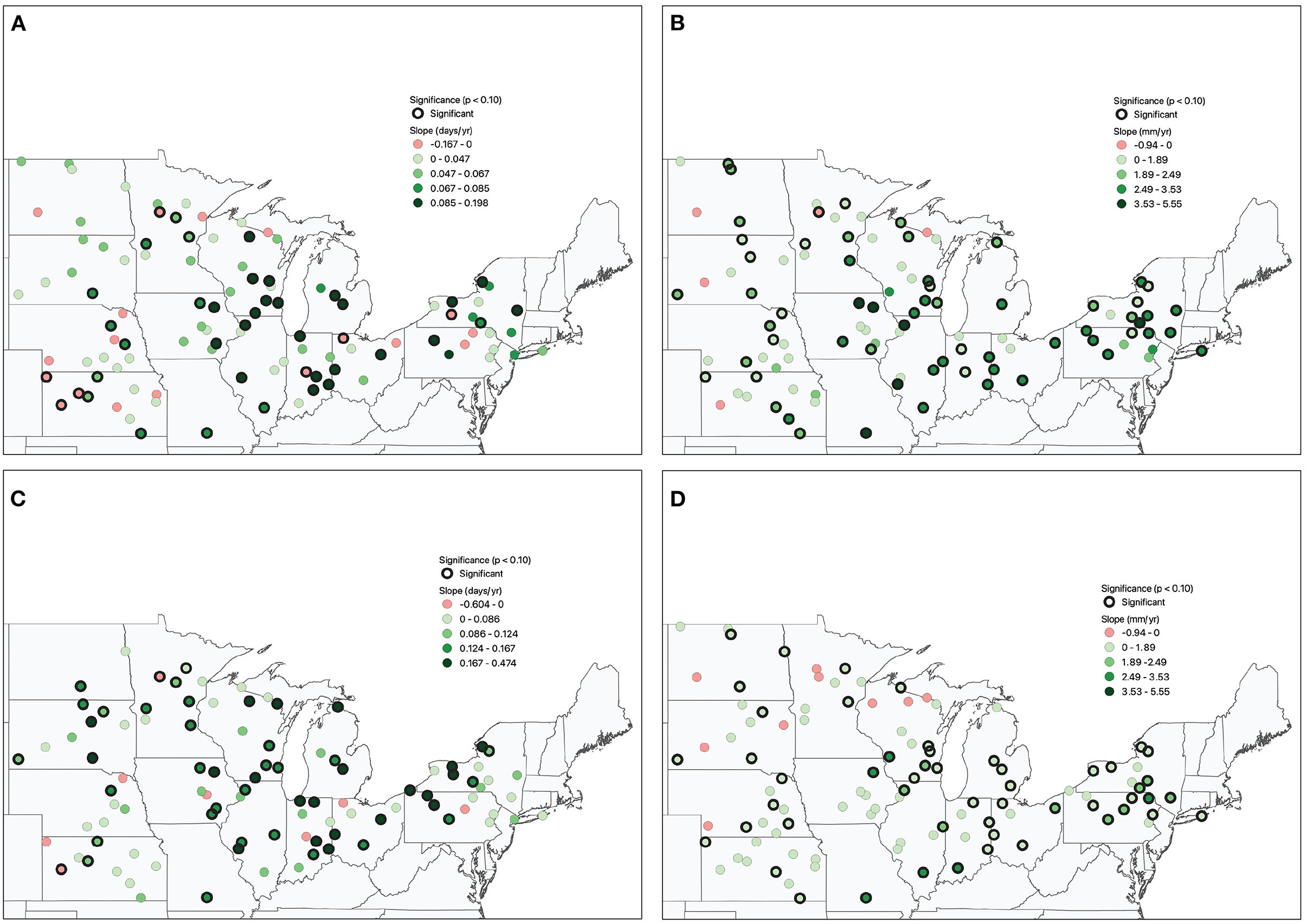
Figure 3. Trends for 1951–2019 in representative annual indicators of precipitation characteristics at locations in the Midwest and Great Lakes region that passed the quality control checks described in the methods section: (A) annual counts of wet-wet day sequences (ANN WW; days; count year−1; upper left), (B) annual total precipitation on wet days (PRCPTOT; mm year−1; upper right), (C) number of days with precipitation ≥ 1.26 mm (R1.26mm; days year−1; lower left), and (D) total precipitation on days when precipitation is ≥ 95th percentile (R95pTOT; mm year−1; lower right).
We also evaluated the ratio of the trend estimates for the annual indicators of R95pTOT and PRCPTOT for stations with a significant positive trend in PRCPTOT, as an indicator of the relative contribution of precipitation on very wet days to trends in total precipitation (Supplementary Figure 3). In general, precipitation on very wet days has contributed the most (ratios >0.60 and at some locations >1.0) to annual total precipitation in eastern New York/Pennsylvania, Indiana, southern Wisconsin/eastern Iowa, and eastern Nebraska/Kansas, compared to elsewhere in the study region. The modest (<0.60) ratios at many locations elsewhere suggest that the overall increase in total precipitation is not exclusively, or even primarily, tied to increases in the frequency of higher intensity events. Rather, changes in the frequency of lighter accumulations are also contributing to the trends in total precipitation.
To better understand the consistency at individual locations of the trends across precipitation indicators, a four-sided Venn diagram was used to plot the number of significant positive trends and the percentage of significant positive trends for all possible combinations of the four representative precipitation indicators, PRCPTOT, WW, R1.26 mm, and R95pTOT, recognizing that the number of available stations varies among indicators due to differing frequency of breakpoints identified in the time series (Figure 4). The number of locations with significant positive trends for multiple indicators is substantial, with 16.3% of the stations with positive trends for all the indicators considered and 19.8% stations with positive trends for the two accumulation indicators PRCPTOT and R95pTOT. The number of stations with significant trends for the three variable combinations and the other two variable combinations is relatively small.

Figure 4. Venn Diagram of the number of stations with significant positive trends for all possible combinations of four representative annual precipitation indicators: the probability of wet-wet days (WW), total annual precipitation (PRCPTOT), the number of wet days (R1.26mm), total precipitation on days with precipitation ≥ 95th percentile (R95pTOT). Percentages are relative to largest number of significant positive trends which was 86. Percentage of significant (p ≤ 0.10) positive trends falling in each category is shown in parentheses.
Seasonal Indicators
For brevity, seasonal results are shown only for PRCPTOT, R95pTOT, WW, and R1.26 mm, which capture the breadth of the different precipitation indicators. As for the annual precipitation characteristics, we observe that in all seasons the number of significant positive trends at all significance thresholds considered substantially exceeds the number of significant negative trends for the selected indicators (Table 3). However, the proportion of stations with significant trends varies by season. The seasonal trends for PRCPTOT indicate that no single season is solely responsible for the annual increase in precipitation observed at the majority of the stations. Significant (p ≤ 0.10) positive trends are observed at over 35% of the stations in fall and winter, 30% of the stations in summer, and 20% of stations in spring. With the exception of one location in winter, no significant negative trends in seasonal PRCPTOT are evident. For R95pTOT, significant positive trends are evident at 33% of the stations in fall but at only approximately 20% of stations in the other seasons. For WW, over 24% percent of the station locations have significant positive trends in summer, fall, and winter, whereas only 15% of all stations observed in spring have positive trends. When the threshold for significance is weaker (p < 0.20), the number of significant trends increases substantially for most indicators in most seasons. Almost all of the additional significant trends that emerge by lowering the threshold are positive in sign. The number of significant trends in any one season is typically less than the number of significant trends for the corresponding annual indicator. Under the weak (p ≤ 0.20) threshold, no individual seasonal indicator presents significantly positive trends at more than 50% of stations, with the exception of R1.26 mm in fall Similar to the annual indicators, when the threshold for significance is stricter (p ≤ 0.05), fewer stations exhibit statistically positive trends, while the number of statistically significant negative trends remains largely unchanged.
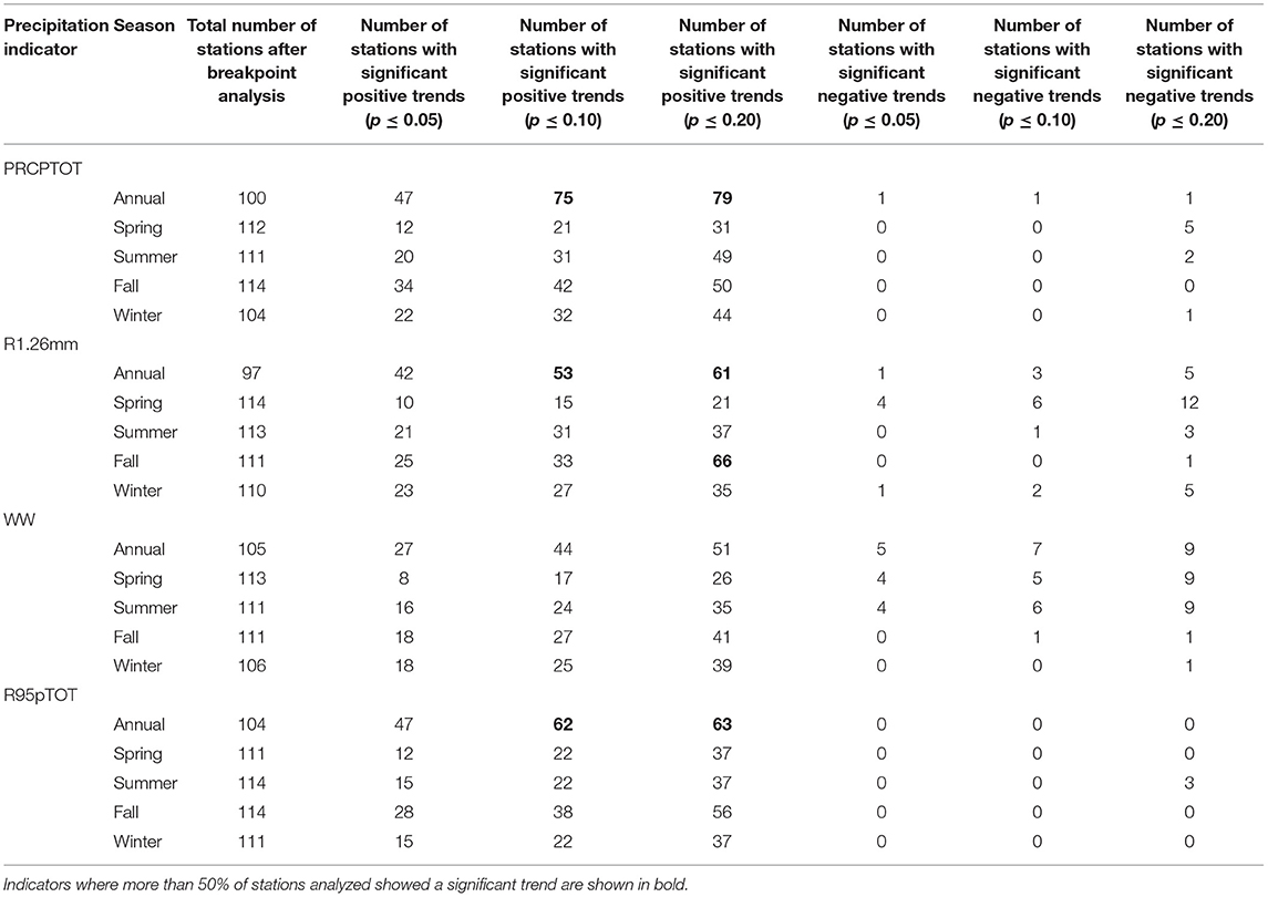
Table 3. Number of stations exhibiting statistically significant trends (Mann Kendall, p ≤ 0.05 two-tailed, p ≤ 0.10 two-tailed, p ≤ 0.20, two-tailed) from 1951 to 2019 in four representative seasonal indicators: total seasonal precipitation (PRCPTOT), the number of wet days (R1.26mm), the count of wet-wet days (WW), and the total precipitation on days with precipitation ≥ 95th percentile (R95pTOT).
Seasonal variations in the spatial patterns in trends over time are shown for PRCPTOT, R95pTOT, and WW. The spatial distributions for R1.26 mm are not shown as they are similar to those for WW. Large between season differences in the spatial variability of the temporal trends are evident. For instance, locations with significant (p ≤ 0.10) positive trends in seasonal PRCPTOT are distributed across the study area in fall but are largely confined to the vicinity of the Great Lakes (Wisconsin, the Lower Peninsula of Michigan, northeastern Ohio, western Pennsylvania, western New York) in winter (Figure 5). In spring, most of the significant positive trends are found in the western two thirds of the study region with few significant trends in New York, Pennsylvania, and Ohio, whereas in summer the greatest density of significant trends along with the largest trend magnitudes are found in the eastern and central portions of the study region. For most stations, significant positive trends are observed in only one or two seasons. A significant negative trend across all seasons is observed at only one location.

Figure 5. Trends (mm year−1) in seasonal total precipitation (PRCPTOT) for: (A) spring, (B) summer, (C) fall, and (D) winter.
The seasonal trends of R95pTOT display less spatial coherence when compared to seasonal PRCPTOT and to annual R95pTOT, with locations with significant positive trends often surrounded by locations with insignificant positive, and sometimes insignificant negative, trends (Figure 6). The number of locations in winter with significant positive trends is relatively small and these locations are mostly found in the vicinity of the western Great Lakes. The spatial extent of significant positive trends expands in spring to include most of the southern and eastern portions of the study area, with few significant trends evident in the northwestern portion of the study area. In summer, locations with significant positive trends are clustered in New York/Pennsylvania, Ohio/Indiana, and southern Wisconsin. The largest magnitude trends in R95pTOT are generally observed during the summer months. Significant positive trends are evident in fall across much of the area except for the extreme western portion of the study region and in the Lower Peninsula of Michigan. Although negative trends are evident for a number of locations in all seasons for R95pTOT, these trends are significant at only one location in spring and two locations in winter.
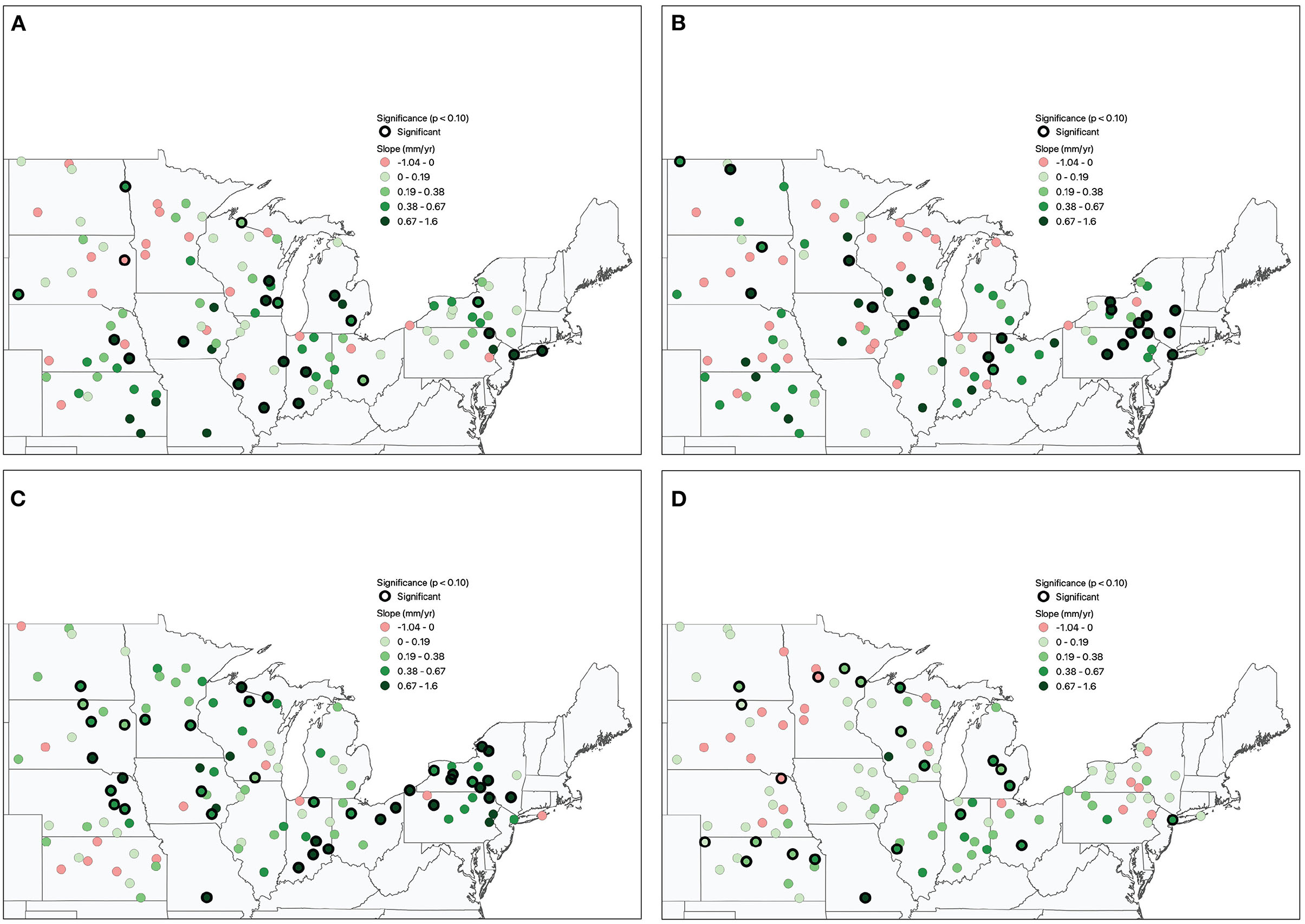
Figure 6. Trends (mm year−1) in the seasonal amount of total precipitation falling on days with precipitation ≥ 95th percentile (R95pTOT) for (A) spring, (B) summer, (C) fall, and (D) winter.
Significant trends in seasonal WW are less spatially coherent than the annual WW indicator (Figure 7). As with seasonal R95pTOT, significant positive trends are often surrounded by insignificant trends or in a few cases significant negative trends. In general, stations with significant positive trends are more clustered for WW than for seasonal R95pTOT but less so than for seasonal PRCPTOT. The number of stations with significant positive trends is small in spring, and there are several (5) significant negative trends. The stations with significant positive trends are relatively dispersed, although some clustering is evident near the center of the study region. A more distinct spatial pattern is present in summer. Stations with significant positive trends are concentrated in Iowa, Indiana, Wisconsin, Ohio, Pennsylvania, and New York. In contrast, mostly insignificant trends are evident throughout the Plains states and east across Minnesota and northern Wisconsin, and the few significant trends in this area are negative. In fall, significant positive trends in WW are found across the northern half of the study region, whereas mostly insignificant trends of mixed sign are observed for the southern half of the region with the exception of Illinois. Little spatial coherence is evident in the wintertime trends of WW, other than some clustering of significant positive trends in the central and extreme northeast sections of the study region.
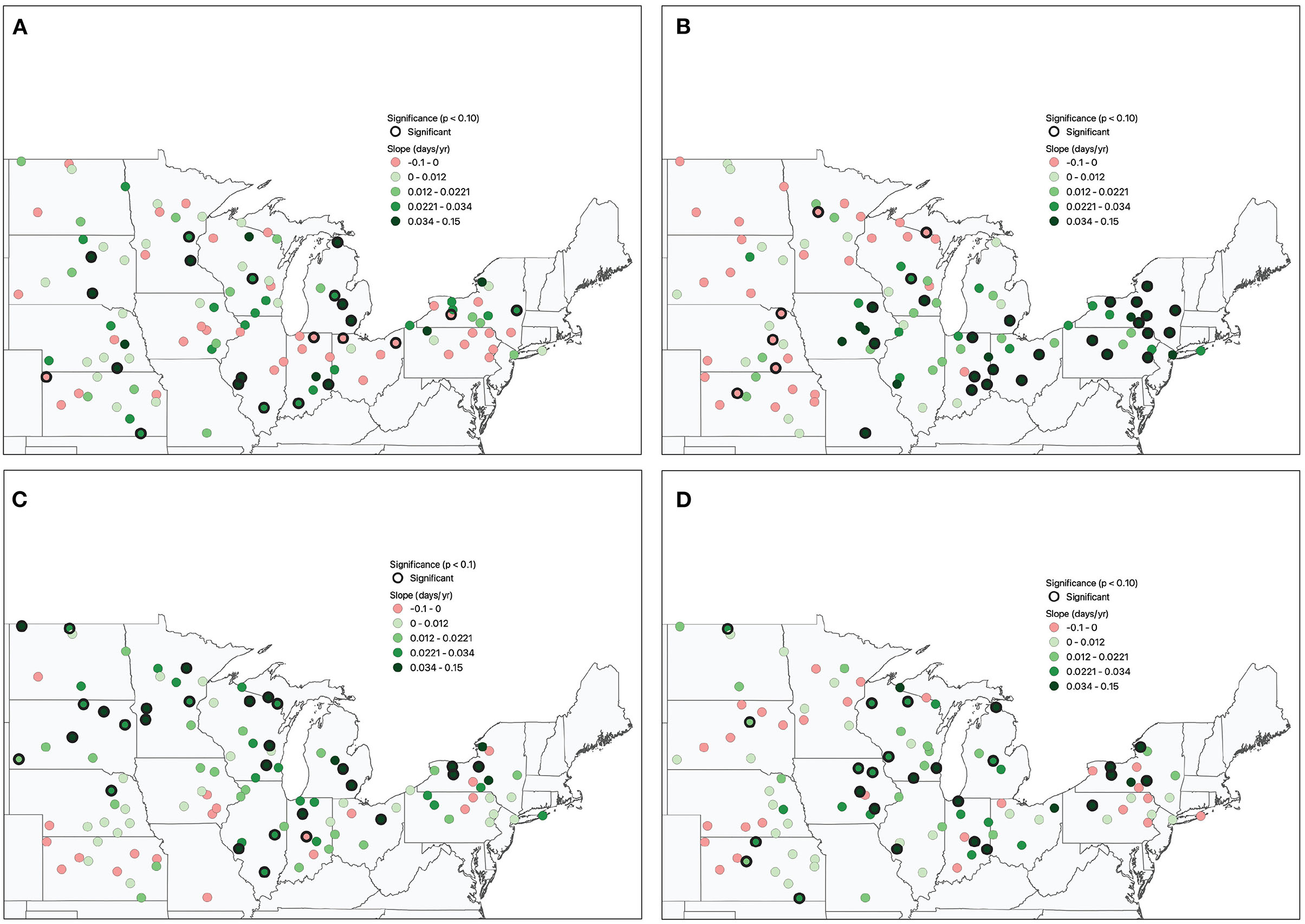
Figure 7. Trends (days year−1) in the seasonal count of wet-wet-day sequences (WW) for (A) spring, (B) summer, (C) fall, and (D) winter.
When compared to annual indicators, the Venn diagrams of seasonal indicators show that the groupings of indicators are more dispersed among the possible combinations of the four representative indicators (Supplementary Figure 4). In fall and winter the three-indicator combination of PRCPTOT, WW, and R1.26MM and the two-indicator combination of PRCPTOT and R95pTOT are more frequent, while in summer the most common combination is PRCPTOT and R1.26MM. In spring, locations are less likely compared to the other seasons to experience significant positive trends for two or more of the representative precipitation indicators, in part a reflection the smaller number of significant trends. For all seasons except spring a substantial number of stations display a significant trend only for R95pTOT. Venn diagrams can also be used to assess whether individual locations are likely to experience significant trends in a particular indicator during more than one season. Our results indicate that, regardless of the indicator type, significant positive trends are most likely to be observed during only one season (Supplementary Figure 5).
Total Precipitable Water
Trends in annual daily mean TOTPRCPWAT during the 1951–2019 study period are positive in sign and significant over the southern two-thirds of the study region (Figure 8). The largest trends are in the south-central portion of the study region with the smallest trends located over the central and western Great Lakes. A significant increase in TOTPRCPWAT is also evident over the Great Plains, with the magnitude of the trend decreasing from south to north. Correlations between the trends in annual TOTPRCPWAT and the trends in the annual values of the four representative precipitation indicators are weak to moderate (Table 4 and Supplementary Figure 6), as indicated by the parametric Pearson's r and non-parametric Kendall's τ correlation coefficients. Correlations for the annual trends are insignificant (p ≤ 0.05) and negative for WW and R1.26 mm, and insignificant but positive for PRCPTOT. Only the correlation between the annual trends in TOTPRCPWAT and those in R95pTOT is significant, with the sign of the correlation indicating a positive association between the annual trends of these two variables.
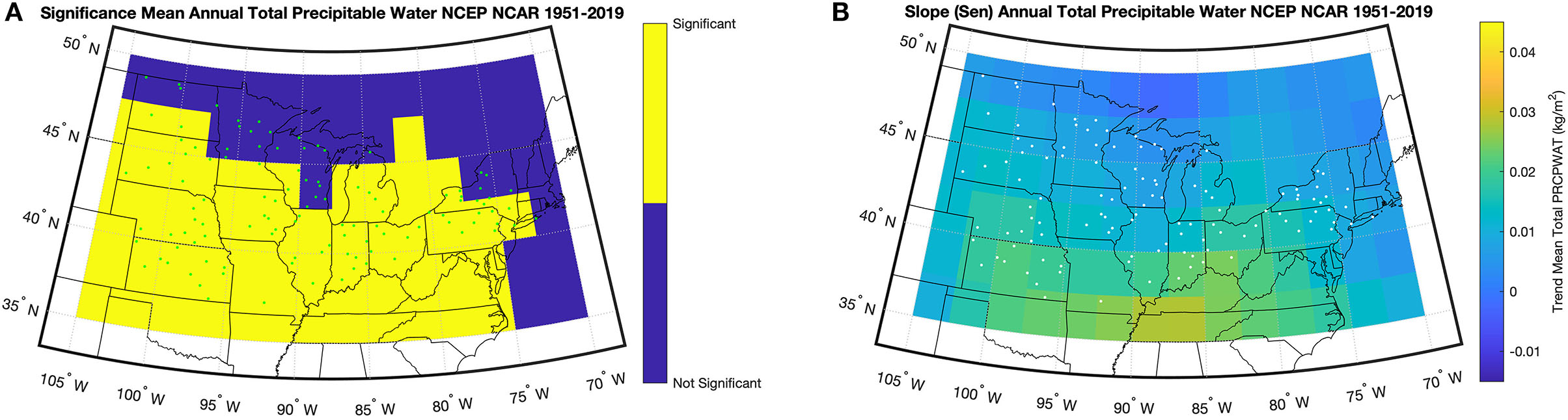
Figure 8. (A) Significance (p ≤ 0.05) and (B) Sen's slope (kg m−2 yr-1) of the trend in annual mean daily total precipitable water for the study region from 1951 to 2019. The stations with quality-controlled precipitation time series are shown on both maps as dots.

Table 4. Pearson correlation coefficients (r) and Kendall rank correlation coefficients (τ) between annual and seasonal trends from 1951 to 2019 in precipitation indicators and total precipitable water.
Assessment of the possible contribution of seasonal trends in TOTPRCPWAT to seasonal trends in the representative precipitation indicators is complicated by seasonal variations in the significance of the TOTPRCPWAT trends, although in general correlation coefficients at the seasonal time scale are larger than those at the annual scale. Significant (p ≤ 0.05) positive trends in TOTPRCPWAT (Supplementary Figure 7) are evident during spring, summer, and fall for portions of the study area, although insignificant trends are observed for a substantial number of the reanalysis grid cells, with the location of the insignificant trends varying by season. In contrast, trends in TOTPRCPWAT are insignificant for all grid cells in winter. Most of the significant (p = 0.05) correlations between the seasonal trends in TOTPRCPWAT and the season trends in the precipitation indicators are positive, although the significance of the trends varies by season and indicator. Correlations between the seasonal trends are significant in spring (PRCPTOT, R1.26mm, R95pTOT), summer (WW, PRCPTOT, R1.26mm, R95pTOT), and winter (PRCPTOT and R95pTOT), although the significant winter trends should be treated cautiously given the weak trends in TOTPRCPWAT at this time of year. No significant correlations were observed in the fall under Pearson's r. When Kendall's τ is used, correlations for fall are significant and negative for PRCPTOT and R95pTOT.
Discussion/Conclusion
The impact of the additional quality control measures on the number of stations available for precipitation trend analysis is striking. Of the 317 stations in the Midwest and Great Lakes region that met the initial criterion of 90% completeness, 203 stations were removed at the second step because they failed the tests for observer bias (underreporting of precipitation ≤ 1.26 mm and over-reporting of precipitation amounts divisible by 5 or 10 when precipitation is recorded in inches). In contrast, the breakpoint analyses, which were conducted separately for each precipitation indicator in recognition that discontinuities can impact the indicators differently, removed only a small portion of the remaining stations (17 or fewer, depending on the indicator). This is a somewhat surprising result given the well-documented discontinuities in observations from the United States Cooperative Observer Network (Karl et al., 1987; Winkler, 2004; Menne et al., 2010), which is the largest source of precipitation data for the United States in the GHCN-D database (Menne et al., 2012). One interpretation is that many of the precipitation time series were affected by both observer bias and discontinuities and were removed following the tests for observation bias. The number of stations with breakpoints was largest for the “accumulation” and “threshold” precipitation indicators, suggesting the tests for observation bias did not remove all afflicted time series for these indicators. The final suite of quality-controlled time series has a much coarser station density than the datasets used in previous studies, and, while not suitable for investigating local-scale variations in precipitation trends, provides high confidence in the estimation of regional-scale variations. The quality-control routines implemented here also allow for more confidence in trends across the range of indicators from high frequency light events to low frequency extreme events, as observer bias affects various indicators differently and may not be captured in studies relying solely on data completeness and documented changes for data screening.
One finding from the use of the carefully quality-controlled time series is that the estimated trends for 1951–2019 in the Midwest and Great Lakes region are predominantly positive for all the “wet” precipitation indicators and negative for the “dry” precipitation indicators. In fact, there is a near absence of significant negative trends across the region for all indicators, with the exception of DD and CDD, and for all seasons and at all three significance levels included in the analysis. On the other hand, the proportion of stations with significant positive trends varies by precipitation indicator, season, and significance level. In general, significant trends at the moderate (p ≤ 0.10) significance level are most likely for the indicators involving precipitation accumulation and counts of days with precipitation above specified thresholds, and less likely for indicators of maximum reported precipitation and the indictors defined in terms of the sequencing of precipitation. Thus, users need to be cautious of inferring from significant trends in common precipitation characteristics, such as total precipitation, that significant trends are also occurring in other precipitation characteristics at a particular location. The larger number of significant positive trends for the “wet” indicators under the weak (p ≤ 0.20) significant level obviously need to be interpreted cautiously because of the greater probability of a Type I error (rejecting the null hypothesis of no trend when it is true). However, the greater spatial coherence of the locations with significant trends for the weak significance level compared to the moderate and stringent levels is consistent with a regional-scale trend toward a wetter climate that is emerging from interannual variability.
Our results also confirm that precipitation indicators that are defined annually often mask strong seasonal variations in the temporal trends of both high frequency, low magnitude events and low frequency, high magnitude events. For almost all locations, one cannot assume based on the trends in an annual precipitation indicator that a location is experiencing similar trends seasonally. Instead, a significant trend in a particular precipitation indicator typically is observed during only one season.
While the low spatial density of the stations that met all three of the quality control criteria somewhat constrains inferences regarding subregional variations in precipitation trends, our results, especially those using the weaker and moderate significance levels, suggest that the character of precipitation is not changing uniformly across the Midwest and Great Lakes region. In terms of the annual values of four representative precipitation indicators (PRCPTOT, R1.26mm, WW, R95pTOT), significant positive trends are observed across the central and eastern portions of the study region for all four indicators, whereas in the west there is a notable absence of significant positive trends for R1.26mm events. Seasonal differences in the spatial distribution of significant trends are also evident, particularly for winter when significant trends for the four representative indicators are largely confined to western Great Lakes portion of the study region. The smaller number of significant trends present under the strict criteria, highlights the strength and relative cohesiveness of trends in precipitation in the central and eastern portions of the region, where most of the significant (p ≤ 0.05) trends are located.
The quality-controlled time series are also useful for evaluating relationships between trends in the precipitation characteristics and physical processes potentially contributing to these trends. Expanding on the intriguing findings of Kunkel et al. (2020b) who found a significant positive correlation between regionally-averaged trends in extreme precipitation and trends in precipitable water for the contiguous United States, we correlated, at annual and seasonal temporal scales, the trends in PRCPTOT, R1.26mm, WW, and R95pTOT for the quality-controlled station time series with trends in average daily precipitable water at a 2.5° latitude x 2.5° longitude resolution from the NCEP/NCAR reanalysis (Kalnay et al., 1996). The correlations for R95pTOT support for the Midwest and Great Lakes region the coarser-scale findings from Kunkel et al. (2020a) that the trend in extreme precipitation increases with an increasing trend in precipitable water, but also point to a more complex interpretation of the relationship between in trends in precipitation characteristics and trends in precipitable water for the study region. In particular, significant (p ≤ 0.05) correlations are evident during spring and summer for PRCPTOT and R1.26mm and in summer for WW, suggesting that increases in precipitable water may also contribute to positive trends in high frequency precipitation events and even to the sequencing of wet days. Also, the correlation between the trend in R95pTOT and that for precipitable water is insignificant in fall for the parametric correlation coefficient and significant but negative for the non-parametric correlation coefficient, suggesting that changes in atmospheric lifting mechanisms (e.g., fronts, extratropical cyclones) rather than increased atmospheric humidity may be more important for explaining the positive trend in R95pTOT in the Midwest and Great Lakes region in fall. Our findings of insignificant trends in precipitable water for large portions of the study area, especially in winter when the precipitable water trends are insignificant for the entire NCEP/NCAR grid over the study area, point to the need for cautious interpretation of the relationship between trends in precipitable water and trends in precipitation characteristics.
We have demonstrated the usefulness of quality-controlled precipitation time series for evaluating trends in precipitation characteristics and for investigating their relationship with processes. However, the limitations of the quality-controlled dataset should also be considered in interpreting the findings presented here and when applying the time series in future work. A key limitation is the coarse spatial resolution of the quality-controlled time series, limiting their usefulness in investigating potential contributions of local-scale features such as lake surfaces or topography on trends in precipitation characteristics. Another concern is that identified breakpoints in the time series that are attributed to changes in instrumentation, station moves or observation protocols may instead be caused by changes in circulation regimes. Also, some types of precipitation indicators may be less sensitive to observer bias than others, and a less stringent protocol for removing time series for consideration would be appropriate. Moreover, for any quality control routine that is not manual, there are almost always time series with data issues relevant to a particular analysis that pass through filters and checks and those without data issues that are incorrectly removed.
In sum, our analysis focused on quality control of station time series to improve the quality of data prior to analysis. As a result of this effort, the trends in our study tended to exhibit a more cohesive spatial and temporal similarities when compared with studies with different quality control criteria, illustrating the importance of quality control of observations in climatic studies. Also, our results indicate, at least for the Midwest and Great Lakes region, that not only is extreme precipitation increasing but the entire distribution of precipitation has been shifting upward over time.
Data Availability Statement
The original contributions presented in the study are included in the article/Supplementary Material, further inquiries can be directed to the corresponding author/s.
Author Contributions
WB, JA, and JW conceived the research questions, reviewed/edited manuscript drafts, approved of submission, and designed the methodology. WB wrote original manuscript draft, acquired data, conducted analyses, and prepared figures. JA supervised and secured funding for the research. All authors contributed to the article and approved the submitted version.
Funding
Funding for this project was provided by the Great Lakes Integrated Sciences and Assessments Program (GLISA), a collaboration of the University of Michigan and Michigan State University (MSU) funded by the National Oceanic and Atmospheric Administration (NOAA) Oceanic and Atmospheric Research (OAR) office [NOAA-OAR-CPO Grant no. NA15OAR4310148].
Conflict of Interest
The authors declare that the research was conducted in the absence of any commercial or financial relationships that could be construed as a potential conflict of interest.
Publisher's Note
All claims expressed in this article are solely those of the authors and do not necessarily represent those of their affiliated organizations, or those of the publisher, the editors and the reviewers. Any product that may be evaluated in this article, or claim that may be made by its manufacturer, is not guaranteed or endorsed by the publisher.
Supplementary Material
The Supplementary Material for this article can be found online at: https://www.frontiersin.org/articles/10.3389/frwa.2022.817342/full#supplementary-material
References
Alexander, L. V., Zhang, X., Peterson, T. C., Caesar, J., Gleason, B., Klein Tank, A. M. G., et al. (2006). Global observed changes in daily climate extremes of temperature and precipitation. J. Geophys. Res. 111:D05109. doi: 10.1029/2005JD006290
Angel, J., Swanston, C., Boustead, B. M., Conlon, K. C., Hall, K. R., Jorns, J. L., et al. (2018). “Midwest,” in Impacts, Risks, and Adaptation in the United States: Fourth National Climate Assessment, Volume II, eds D. R. Reidmiller, C. W. Avery, D. R. Easterling, K. E. Kunkel, K. L. M. Lewis, T. K. Maycock, and B. C. Stewart (Washington, DC: U.S. Global Change Research Program). doi: 10.7930/NCA4.2018.CH21
Attavanich, W., McCarl, B. A., Ahmedov, Z., Fuller, S. W., and Vedenov, D. V. (2013). Effects of climate change on US grain transport. Nat. Clim. Chang. 37, 638–643. doi: 10.1038/nclimate1892
Bartels, R. J., Black, A. W., and Keim, B. D. (2020). Trends in precipitation days in the United States. Int. J. Climatol. 40, 1038–1048. doi: 10.1002/joc.6254
Baule, W. J., and Shulski, M. D. (2014). Climatology and trends of wind speed in the Beaufort/Chukchi Sea coastal region from 1979 to 2009. Int. J. Climatol. 34:3881. doi: 10.1002/joc.3881
Bell, G. D., and Janowiak, J. E. (1995). Atmospheric circulation associated with the midwest floods of 1993. Bull. Am. Meteorol. Soc. 76, 681–695. doi: 10.1175/1520-0477(1995)076<0681:ACAWTM>2.0.CO;2
Bowles, T. M., Atallah, S. S., Campbell, E. E., Gaudin, A. C. M., Wieder, W. R., and Grandy, A. S. (2018). Addressing agricultural nitrogen losses in a changing climate. Nat. Sustain. 1, 399–408. doi: 10.1038/s41893-018-0106-0
Chin, N., Byun, K., Hamlet, A. F., and Cherkauer, K. A. (2018). Assessing potential winter weather response to climate change and implications for tourism in the U.S. Great Lakes and Midwest. J. Hydrol. Reg. Stud. 19, 42–56. doi: 10.1016/J.EJRH.2018.06.005
Contractor, S., Donat, M. G., and Alexander, L. V. (2021). Changes in observed daily precipitation over global land areas since 1950. J. Clim. 34, 3–19. doi: 10.1175/JCLI-D-19-0965.1
Costa, A. C., and Soares, A. (2009). Homogenization of climate data: review and new perspectives using geostatistics. Math. Geosci. 41, 291–305. doi: 10.1007/s11004-008-9203-3
Dai, S., Shulski, M. D., Hubbard, K. G., and Takle, E. S. (2016). A spatiotemporal analysis of Midwest US temperature and precipitation trends during the growing season from 1980 to 2013. Int. J. Climatol. 36, 517–525. doi: 10.1002/joc.4354
Daly, C., Conklin, D. R., and Unsworth, M. H. (2010). Local atmospheric decoupling in complex topography alters climate change impacts. Int. J. Climatol. 30, 1857–1864. doi: 10.1002/JOC.2007
Daly, C., Gibson, W. P., Taylor, G. H., Doggett, M. K., and Smith, J. I. (2007). Observer bias in daily precipitation measurements at United States Cooperative Network Stations. Bull. Am. Meteorol. Soc. 88, 899–912. doi: 10.1175/BAMS-88-6-899
Donat, M. G., Alexander, L. V., Yang, H., Durre, I., Vose, R., Caesar, J., et al. (2013). Global land-based datasets for monitoring climatic extremes. Bull. Am. Meteorol. Soc. 94, 997–1006. doi: 10.1175/BAMS-D-12-00109.1
Durre, I., Menne, M. J., Gleason, B. E., Houston, T. G., and Vose, R. S. (2010). Comprehensive automated quality assurance of daily surface observations. J. Appl. Meteorol. Climatol. 49, 1615–1633. doi: 10.1175/2010JAMC2375.1
Durre, I., Menne, M. J., and Vose, R. S. (2008). Strategies for evaluating quality assurance procedures. J. Appl. Meteorol. Climatol. 47, 1785–1791. doi: 10.1175/2007JAMC1706.1
Easterling, D. R. (2002). United States Historical Climatology Network Daily Temperature and Precipitation Data (1871-1997). Oak Ridge, TN: Oak Ridge National Laboratory.
Groisman, P. Y., Karl, T. R., Easterling, D. R., Knight, R. W., Jamason, P. F., Hennessy, K. J., et al. (1999). Changes in the probability of heavy precipitation: important indicators of climatic change. Clim. Change 42, 243–283. doi: 10.1023/A:1005432803188
Groisman, P. Y., and Knight, R. W. (2008). Prolonged dry episodes over the conterminous United States: New tendencies emerging during the last 40 years. J. Clim. 21, 1850–1862. doi: 10.1175/2007JCLI2013.1
Gronewold, A. D., Do, H. X., Mei, Y., and Stow, C. A. (2021). A tug-of-war within the hydrologic cycle of a continental freshwater basin. Geophys. Res. Lett. 48:e2020GL090374. doi: 10.1029/2020GL090374
Guilbert, J., Betts, A. K., Rizzo, D. M., Beckage, B., and Bomblies, A. (2015). Characterization of increased persistence and intensity of precipitation in the northeastern United States. Geophys. Res. Lett. 42, 1888–1893. doi: 10.1002/2015GL063124
Gutowski, W. J., Willis, S. S., Patton, J. C., Schwedler, B. R. J., Arritt, R. W., and Takle, E. S. (2008). Changes in extreme, cold-season synoptic precipitation events under global warming. Geophys. Res. Lett. 35:L20710. doi: 10.1029/2008GL035516
Higgins, R. W., Silva, V. B. S., Shi, W., and Larson, J. (2007). Relationships between climate variability and fluctuations in daily precipitation over the United States. J. Clim. 20, 3561–3579. doi: 10.1175/JCLI4196.1
Hoerling, M., Eischeid, J., Perlwitz, J., Quan, X. W., Wolter, K., and Cheng, L. (2016). Characterizing recent trends in U.S. heavy precipitation. J. Clim. 29, 2313–2332. doi: 10.1175/JCLI-D-15-0441.1
Huang, H., Winter, J. M., and Osterberg, E. C. (2018). Mechanisms of abrupt extreme precipitation change over the Northeastern United States. J. Geophys. Res. Atmos. 123, 7179–7192. doi: 10.1029/2017JD028136
Huang, H., Winter, J. M., Osterberg, E. C., Horton, R. M., and Beckage, B. (2017). Total and extreme precipitation changes over the Northeastern United States. J. Hydrometeorol. 18, 1783–1798. doi: 10.1175/JHM-D-16-0195.1
Hunt, E. D., Birge, H. E., Laingen, C., Licht, M. A., McMechan, J., Baule, W., et al. (2020). A perspective on changes across the U.S. Corn Belt. Environ. Res. Lett. 15:071001. doi: 10.1088/1748-9326/ab9333
Ines, A. V. M., Hansen, J. W., and Robertson, A. W. (2011). Enhancing the utility of daily GCM rainfall for crop yield prediction. Int. J. Climatol. 31, 2168–2182. doi: 10.1002/joc.2223
Jaiswal, R. L., Lohaniu, A. K., and Tiwari, H. L. (2015). Statistical analysis for change detection and trend assessment in climatological parameters. Environ. Processes. 2, 729–749. doi: 10.1007/s40710-015-0105-3
Janssen, E., Wuebbles, D. J., Kunkel, K. E., Olsen, S. C., and Goodman, A. (2014). Observational- and model-based trends and projections of extreme precipitation over the contiguous United States. Earth's Futur. 2, 99–113. doi: 10.1002/2013EF000185
Kalnay, E., Kanamitsu, M., Kistler, R., Collins, W., Deaven, D., Gandin, L., et al. (1996). The NCEP/NCAR 40-year reanalysis project. Bull. Am. Meteorol. Soc. 77, 437–471. doi: 10.1175/1520-0477(1996)077<0437:TNYRP>2.0.CO;2
Karl, T. R., Williams, C. N., and Karl, T. R. (1987). An approach to adjusting climatological time series for discontinuous inhomogeneities. J. Clim. Appl. Meteorol. 26, 1744–1763. doi: 10.1175/1520-0450(1987)026<1744:AATACT>2.0.CO;2
Kiefer, M. T., Andresen, J. A., McCullough, D. G., Baule, W. J., and Notaro, M. (2021). Extreme minimum temperatures in the Great Lakes region of the United States: A climatology with implications for insect mortality. Int. J. Climatol. 33, 1585–1600. doi: 10.1002/JOC.7434
Komoto, K., Soldo, L., Tang, Y., Chilvers, M. I., Dahlin, K., Guentchev, G., et al. (2021). Climatology of persistent high relative humidity: An example for the Lower Peninsula of Michigan, USA. Int. J. Climatol. 41, E2517–E2536. doi: 10.1002/JOC.6861
Konrad, C. E. (2001). The most extreme precipitation events over the Eastern United States from 1950 to 1996: considerations of scale. J. Hydrometeorol. 2, 309–325. doi: 10.1175/1525-7541(2001)002<0309:TMEPEO>2.0.CO;2
Kunkel, K. E., Karl, T. R., Squires, M. F., Yin, X., Stegall, S. T., and Easterling, D. R. (2020b). Precipitation extremes: trends and relationships with average precipitation and precipitable water in the contiguous United States. J. Appl. Meteorol. Climatol. 59, 125–142. doi: 10.1175/JAMC-D-19-0185.1
Kunkel, K. E., Stevens, S. E., Stevens, L. E., and Karl, T. R. (2020a). Observed climatological relationships of extreme daily precipitation events with precipitable water and vertical velocity in the contiguous United States. Geophys. Res. Lett. 47:e2019GL086721. doi: 10.1029/2019GL086721
Legates, D. R., and Willmott, C. J. (1990). Mean seasonal and spatial variability in gauge-corrected, global precipitation. Int. J. Climatol. 10, 111–127. doi: 10.1002/joc.3370100202
Mallakpour, I., and Villarini, G. (2016). A simulation study to examine the sensitivity of the Pettitt test to detect abrupt changes in mean. Hydrol. Sci. J. 61, 245–254. doi: 10.1080/02626667.2015.1008482/SUPPL_FILE/THSJ_A_1008482_SM3561.DOC
Mallakpour, I., and Villarini, G. (2017). Analysis of changes in the magnitude, frequency, and seasonality of heavy precipitation over the contiguous USA. Theor. Appl. Climatol. 130, 345–363. doi: 10.1007/s00704-016-1881-z
Menne, M. J., Durre, I., Vose, R. S., Gleason, B. E., and Houston, T. G. (2012). An overview of the global historical climatology network-daily database. J. Atmos. Ocean. Technol. 29, 897–910. doi: 10.1175/JTECH-D-11-00103.1
Menne, M. J., Williams, C. N., and Palecki, M. A. (2010). On the reliability of the U.S. surface temperature record. J. Geophys. Res. Atmos. 115:11108. doi: 10.1029/2009JD013094
Myhre, G., Forster, P. M., Samset, B. H., Hodnebrog, Ø., Sillmann, J., Aalbergsjø, S. G., et al. (2016). PDRMIP: A precipitation driver and response model intercomparison project, protocol and preliminary results. Bull. Am. Meteorol. Soc. 98, 1185–1198. doi: 10.1175/BAMS-D-16-0019.1
Onyutha, C. (2021). Graphical-statistical method to explore variability of hydrological time series. Hydrol. Res. 52, 266–283. doi: 10.2166/NH.2020.111
Pettitt, A. N. (1979). A non-parametric approach to the change-point problem. Appl. Stat. 28, 126–135.
Pielke, R. A., and Downton, M. W. (2000). Precipitation and damaging floods: Trends in the United States, 1932–1997. J. Clim. 2000, 3625–3637. doi: 10.1175/1520-0442(2000)013<3625:PADFTI>2.0.CO;2
Pryor, S. C., Howe, J. A., and Kunkel, K. E. (2009). How spatially coherent and statistically robust are temporal changes in extreme precipitation in the contiguous USA? Int. J. Climatol. 29, 31–45. doi: 10.1002/joc.1696
Riha, S. J., Wilks, D. S., and Simoens, P. (1996). Impact of temperature and precipitation variability on crop model predictions. Clim. Change 32, 293–311. doi: 10.1007/BF00142466
Roque-Malo, S., and Kumar, P. (2017). Patterns of change in high frequency precipitation variability over North America. Sci. Rep. 7:10853. doi: 10.1038/s41598-017-10827-8
Rosenzweig, C., Tubiello, F. N., Goldberg, R., Mills, E., and Bloomfield, J. (2002). Increased crop damage in the US from excess precipitation under climate change. Glob. Environ. Chang. 12, 197–202. doi: 10.1016/S0959-3780(02)00008-0
Schoof, J. T., Pryor, S. C., and Surprenant, J. (2010). Development of daily precipitation projections for the United States based on probabilistic downscaling. J. Geophys. Res. Atmos. 115:D13106. doi: 10.1029/2009JD013030
Sen, P. K. (1968). Estimates of the regression coefficient based on Kendall's Tau. J. Am. Stat. Assoc. 63:1379. doi: 10.2307/2285891
Sen, Z. (2015). Innovative trend significance test and applications. Theor. Appl. Climatol. 127, 939–947. doi: 10.1007/S00704-015-1681-X
Shulski, M. D., Baule, W., Stiles, C., and Umphlett, N. (2015). A historical perspective on Nebraska's variable and changing climate. Gt. Plains Res. 25:23. doi: 10.1353/gpr.2015.0023
Sneyers, R. (1990). On the Statistical Analysis of Series of Observations. Geneva: Secretariat of the World Meteorological Organization.
Takle, E. S., and Gutowski, W. J. (2020). Iowa's agriculture is losing its Goldilocks climate. Phys. Today 73:26. doi: 10.1063/PT.3.4407
Talukder, B., and Hipel, K. W. (2020). Diagnosis of sustainability of trans-boundary water governance in the Great Lakes basin. World Dev. 129:104855. doi: 10.1016/J.WORLDDEV.2019.104855
Trenberth, K. E., Dai, A., Rasmussen, R. M., and Parsons, D. B. (2003). The changing character of precipitation. Bull. Am. Meteorol. Soc. 84, 1205–1217. doi: 10.1175/BAMS-84-9-1205
Trenberth, K. E., Fasullo, J., and Smith, L. (2005). Trends and variability in column-integrated atmospheric water vapor. Clim. Dyn. 24, 741–758. doi: 10.1007/S00382-005-0017-4/FIGURES/15
Villarini, G., Smith, J. A., Baeck, M. L., Vitolo, R., Stephenson, D. B., and Krajewski, W. F. (2011). On the frequency of heavy rainfall for the midwest of the United States. J. Hydrol. 400, 103–120. doi: 10.1016/j.jhydrol.2011.01.027
Walsh, J., Wuebbles, D., Hayhoe, K., Kossin, J., Kunkel, K., Stephens, G., et al. (2014). Ch. 2: Our Changing Climate. Climate Change Impacts in the United States: The Third National Climate Assessment.
Wang, X. L., Chen, H., Wu, Y., Feng, Y., Pu, Q., Wang, X. L., et al. (2010). New techniques for the detection and adjustment of shifts in daily precipitation data series. J. Appl. Meteorol. Climatol. 49, 2416–2436. doi: 10.1175/2010JAMC2376.1
Weaver, S. J., and Nigam, S. (2008). Variability of the great plains low-level jet: large-scale circulation context and hydroclimate impacts. J. Clim. 21, 1532–1551. doi: 10.1175/2007JCLI1586.1
Williams, C. N., Menne, M. J., and Thorne, P. W. (2012). Benchmarking the performance of pairwise homogenization of surface temperatures in the United States. J. Geophys. Res. Atmos. 117:16. doi: 10.1029/2011JD016761
Winkler, J. A. (1988). Climatological characteristics of summertime extreme rainstorms in Minnesota. Ann. Assoc. Am. Geogr. 78, 57–73.
Winkler, J. A. (2004). “The impact of technology upon in situ atmospheric observations and climate science,” in Geography and Technology (Dordrecht: Springer). doi: 10.1007/978-1-4020-2353-8_20
Wu, S. Y. (2015). Changing characteristics of precipitation for the contiguous United States. Clim. Change 132, 677–692. doi: 10.1007/S10584-015-1453-8/TABLES/2
Zhang, W., and Villarini, G. (2019). On the weather types that shape the precipitation patterns across the U.S. Midwest. Clim. Dyn. 2019, 1–16. doi: 10.1007/s00382-019-04783-4
Keywords: hyrdoclimatology, precipitation, climate change, temporal trend, quality control procedures, regional climatology
Citation: Baule WJ, Andresen JA and Winkler JA (2022) Trends in Quality Controlled Precipitation Indicators in the United States Midwest and Great Lakes Region. Front. Water 4:817342. doi: 10.3389/frwa.2022.817342
Received: 18 November 2021; Accepted: 17 January 2022;
Published: 11 February 2022.
Edited by:
Congsheng Fu, Nanjing Institute of Geography and Limnology, Chinese Academy of Sciences (CAS), ChinaReviewed by:
Semih Kale, Çanakkale Onsekiz Mart University, TurkeyCharles Onyutha, Kyambogo University, Uganda
Copyright © 2022 Baule, Andresen and Winkler. This is an open-access article distributed under the terms of the Creative Commons Attribution License (CC BY). The use, distribution or reproduction in other forums is permitted, provided the original author(s) and the copyright owner(s) are credited and that the original publication in this journal is cited, in accordance with accepted academic practice. No use, distribution or reproduction is permitted which does not comply with these terms.
*Correspondence: William J. Baule, YmF1bGV3aWxAbXN1LmVkdQ==