Salt transport in a large agro-urban river basin: Modeling, controlling factors, and management strategies

Salinity poses a severe threat to urban and agricultural areas. Excess salt can accumulate in soils and groundwater, thereby impacting crop growth and productivity. In this study we quantify the influence of driving forces on salt transport in Colorado's South Platte River (drainage area of 62,937 km²) and investigate possible mediation strategies to reduce salinity levels in both urban and agricultural river reaches. A river salt transport model was developed that utilizes a water allocation model and accounts for multiple inputs and outputs of salt within the river network, including tributaries, wastewater treatment plants, road salt, return flows from rainfall and irrigation, and groundwater discharge. The flow and salt models are run on a monthly basis between 2002 and 2006 and tested against stream discharge and in-stream salinity concentration at multiple gage sites. A sensitivity analysis was implemented to determine the controlling factors behind salt transport in the river system by river reach and by season (spring, summer, fall, winter). SA results were used to guide selection of management practices (n = 256) that can control salinity in both urban and agricultural areas. For urban areas, during spring/summer and fall/winter, the most efficient management practice is to decrease WWTP effluent salinity concentration by 35% and to decrease applied road salt by 35%, respectively, resulting in decreases of 10–30% decrease in river salt concentration. For agricultural areas, the only management practices that achieve an in-river salinity concentration (1,000 mg/L) that prevents crop yield decrease during irrigation are aggressive practices that focus on WWTP effluent concentration, return flow salinity, and urban road salt. Results points to the extreme challenge of managing salinity in the South Platte River Basin and other similar basins and the aggressive urban approaches that must be implemented to sustain irrigation practices in the downstream regions of the basin.

Introduction

Elevated levels of salinity in soils, groundwater, and surface water threatens soil health, crop yield, ecosystem biodiversity, and overall use of water resources (Thorslund and van Vliet, 2020). Salinization can occur by natural (primary) and anthropogenic (secondary) causes. Primary salinity occurs due to weathering of rocks and soils that contain salt minerals (Williams, 1999; Hassani et al., 2020), with resultant mobilized salt minerals dissolved into salt ions and carried via hydrologic pathways (surface runoff, soil lateral flow, groundwater discharge) to streams and lakes. Secondary salinity occurs due to wastewater treatment plant (WWTP) effluent, irrigation practices, mining activities, clearing of vegetation, and application of road salt for deicing (Novotny et al., 2008; Novotny and Stefan, 2010; Cañedo-Argüelles et al., 2013; Asensio et al., 2017; Dugan et al., 2017; Meyer et al., 2020). In many semi-arid river basins that contain both urban and agricultural footprints, both primary and secondary salinization combine to load salt into lakes and river systems. Downstream areas that utilize this salt-laden river water for irrigation can experience decrease in crop yield and overall soil health, pointing to the need for basin-wide management of salinity.

Due to the difficulty in removing salt mass from river water, salinity management in large river basins focuses on, where possible, management of each salinity source. Often, numerical models are used understand the spatio-temporal patterns of salinity movement within the river basins and quantify and predict the impact of management practices on salinity concentrations and loads. Studies thus far, however, have focused mainly on (i) model development, (ii) activies only in agricultural or natural areas, or (iii) activities only in urban areas. Bailey et al. (2019); Maleki et al. (2021); Tirabadi et al. (2021) each developed salinity modules for the SWAT hydrological model (Arnold et al., 1998) for simulating salinity transport at the watershed scale, but only introduced the model, leaving salt management scenario analysis for future studies. Jung et al. (2021) used output from SWAT (streamflow, precipitation, elevation, reach length, soil texture, nutrient loads) and machine learning to predict monthly total dissolved solids in the Rio Grande River, Texas. Huang and Foo (2002) used relationships between freshwater inflows, tidal activity, and wind to predict salinity variation in the Apalochicola River Florida. Hunter et al. (2018) developed a hybrid process-based, data-driven model for predicting river salinity in the Murray River, Australia, focusing on salinity loading from groundwater and floodplain waterbodies in arid agricultural and natural areas. These latter three studies do not investigate model sensitivity or management practices to decrease salinity. Lee et al. (1993) presents a surface water salinity model for the Colorado River and investigates remediation strategies, but only assessed the effects of return flow salinity loads on river quality and reservoir quality. Olson (2019) used empirical models to estimated change in river salinity in the conterminous United States during the twenty first century due to effects of agricultural, industrial, and urban development using spatial data on geology, soil, climate, vegetation, and land use, but did not assess mitigation strategies for salinity.

Tedeschi et al. (2001) applied a hydrosalinity balance model to an irrigation district of the Ebro River Basin in Aragón, Spain to study irrigation and drainage management and their effects on the salt loading, with a focus on irrigation efficiency. Tuteja et al. (2003) used CATSALT, a water balance model linked with a salt transport module, to assess the effect of land use changes on salt loading in a catchment in Australia. Land use scenarios included an increase in pasture content, increase in crop rotations, and an increase in tree cover. Burkhalter and Gates (2006) used the groundwater solute transport model MT3D to assess management practices for reducing groundwater salinity in an irrigated stream-aquifer system in Colorado, USA. Practices include recharge reduction (i.e., increase in irrigation efficiency), canal seepage reduction, installation of subsurface drains, and increase in pumping volumes. Sadoddin et al. (2005) used a Bayesian decision network to assess the ecological consequences of dryland salinity management actions in the Little River Catchment, New South Wales, Australia, including conservation of remnant vegetation, conservation of riparian areas, and drainage. Singh and Panda (2012) used the integrated hydro-salinity model SAHYSMOD to analyze water and salt balances in an irrigated semi-arid area located in the Haryana State of India. Other studies focus on managing salinity in urban areas, such as in optimizing road salt applications (Trenouth et al., 2015; Dietz et al., 2017). In general, however, there remains a need to apply a basin-wide hydro-salinity model to investigate salinity transport and mitigation in river basins that have mixed agro-urban activities, where urban salt pollution can affect agricultural activities, and vice versa.

The objective of this study is to identify management practices that can control in-stream salinity in a large, semi-arid agro-urban river basin. This is accomplished by using an integrated hydro-salinity model to first, quantify the sources of salinity and its transport in the South Platte River, Colorado, USA; second, use sensitivity analysis to identify the system parameters and salinity sources that govern in-stream salinity; and third, use the model to quantify the impact of management practices on in-stream salinity concentration (mg/L) within the Colorado portion of the basin. The integrated model consists of a river network water allocation model, provided by the Colorado Division of Water Resources, and an in-river salt transport model developed for this study. The salinity model accounts for inputs of salt from tributaries, wastewater treatment plants, road salt, returns flows from rainfall and irrigation, and groundwater discharge. The model is tested against in-stream flowrates and salinity concentrations before use in sensitivity analysis and management scenario assessment.

Methods

Study region

The study region for the salinity assessment is the South Platte River Basin (SPRB), a representative semi-arid mixed agro-urban basin that spans three states in the western United States: Colorado (79%), Nebraska (15%), and Wyoming (6%). Figure 1 shows a map of the SPRB, including the spatial extent of the alluvial aquifer system that is in hydraulic connection with the river network. The basin has a drainage area of 62,937 km². The South Platte River begins in central Colorado and flows northeast to Nebraska. Water development in the SPRB began in the 1870s and then expanded rapidly with the construction of diversions, reservoirs, and wells. Cities in the SPRB consist of Denver, Boulder, Longmont, Greeley, Fort Collins, and Cheyenne (see Figure 1), with a total population of about 2.8 million (95% residing in Colorado), resulting in the most concentrated population density in the Rocky Mountain region. A land use map is shown in Figure 2A, indicating the urban areas (red) along the Front Range of the Rocky Mountains.

FIGURE 1

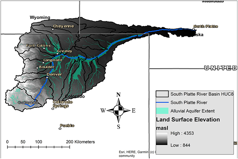
Figure 1. Spatial extent of the South Platte River Basin (SPRB), showing land surface elevation (m above sea level), boundaries of HUC8 subbasins, and extent of the alluvial aquifer.

FIGURE 2

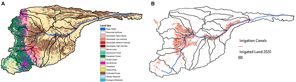
Figure 2. Characteristics of the South Platte River Basin: (A) land use, (B) irrigation canals and irrigated land.

Irrigated agriculture accounts for 8% of land use in the SPRB but more than 70% of water use (Dennehy, 1998). In 2007, the basin accounted for 73% of Colorado's agrarian products (Cook, 2015). The extent of irrigated land and locatios of irrigation canals are shown in Figure 2B. Irrigated areas located far away from irrigation canals receive water from pumping wells (n = 5,074) drilled into the alluvial aquifer (see Figure 1 for alluvial aquifer extent). Irrigation along the alluvial corridors of the river system result in high groundwater levels that drive groundwater discharge into streams (Aliyari et al., 2019). Mountainous areas receive approximately 760 mm (30 in) of precipitation, mostly in the form of snow, whereas the plains east of the Front Range receive 175–380 mm (7–15 in), mainly between April and September.

Salinity levels in the surface water, soil, and groundwater throughout the SPRB have been increasing over the past decades, drastically increasing the risk to crop growth and productivity (NEIRBO, 2020). Salinity levels, measured as total dissolved solids (TDS), in the upper reaches of the South Platte River have increased from 400 mg/L in 1995 to 700 mg/L in 2018 (NEIRBO, 2020). Salinity concentration near the headwaters of the South Platte River has a temporal average of <200 mg/L, increasing to a temporal average of 569 mg/L near the Denver Metro area and increasing throughout the agricultural reaches of the river to 1,165 mg/L near the watershed outlet. As salinized river water moves downstream and is diverted for irrigation (see Figure 2B), there are concerns regarding the impact of salinity on crop yield. A threshold in-river concentration of 1,000 mg/L, corresponding to a water condition that likely will not result in crop yield reduction when applied as irrigation water, is desired for the basin. Recent field sampling studies have found that soils in many agricultural areas have soil salinity levels high enough to be classified as “saline” (Northern Water, 2005). Haby et al. (2000), using a salt mass balance along the agricultural reaches of the South Platte River, concluded that 25% of in-river salinity originated from the Denver metro areas, and 50% was loaded from main tributaries. Other sources include the river system upstream of Denver, and direct surface runoff and groundwater loading.

Model for flow and salt transport in the South Platte River system

Model overview

An integrated hydro-salinity model is developed in this study to simulate the transport of salinity in the South Platte River (see Figure 1) from its headwaters in Colorado to the watershed outlet in Nebraska, flowing through mountains, urban areas, and agricultural areas, a total distance of 563 km.

Simulating streamflow in the South Platte River

The streamflow model uses the Colorado Division of Water Resources (CDWR) StateMod model (https://cdss.colorado.gov/software/statemod, accessed January 2020), a surface water allocation and accounting model for river basins in Colorado. The model simulates stream diversions, in-stream demands, well pumping and recharge (via streamflow depletion and streamflow accretion from pumping and injection, respectively), reservoir operations, water rights augmentation plans, and river flows. The main purpose of the model is to administer water rights in accordance with the prior appreciation doctrine (i.e., first in time, first in right) as a function of water availability, priority, decreed amount, and structure capacity and location. The model is used due to extensive water management practices in the SPRB that have strong influences on spatio-temporal patterns of river discharge.

The StateMod model for the SPRB consists of 1,444 connected nodes. The water allocation network diagram and table of nodal types are shown in Figure 3. The model spans the period 1950–2012, calculating flows in and out of each node on a monthly time step. Sixty six nodes are located along the South Platte River (see map in Figure 3), with flow at these nodes used to simulate streamflow in the South Platte River and compare against flow measurements at USGS gage sites. The flow model includes three main tributaries of the South Platte River: the St. Vrain River, the Big Thompson River, and the Cache la Poudre River (see map in Figure 3). Flow rates from these tributaries were added at the appropriate nodes along the South Platte River. Similarly, effluent flow from the Hite WWTP (see map in Figure 3) (NEIRBO, 2020) was added at the appropriate node. Finally, the amount of groundwater discharge entering the South Platte River between nodes was calculated from model results. This was performed so that spatial variable groundwater salinity concentrations could be assigned to these flow rates, to estimate groundwater salt loading (see Section Simulating salt transport in the South Platte River). The total groundwater flow entering or leaving between a pair of StateMod nodes (see Figure 3) was calculated as the sum of the groundwater flows at each intermediate node between the pair. Similarly, the total return flow between a pair of StateMod nodes was calculated as the sum of the return flows at each intermediate node between the pair.

FIGURE 3

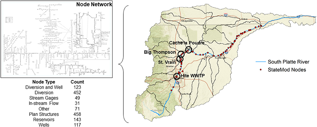
Figure 3. StateMod (water allocation model) node network, listing the various node types and corresponding nodes (red dots) along the South Platte River (see map on right). Inflow locations of major tributaries are shown on the map, as is the location of the major WWTP (Hite WWTP) in the Denver metro area. The Node Network inset diagram is shown for example, and not for detailed interpretation. Black lines on the map indicate boundaries of watersheds at the 8-digit HUC level.

Simulating salt transport in the South Platte River

The salt transport model estimates in-stream salinity concentration (g/m³ = mg/L) throughout the length of the South Platte River (to the Colorado-Nebraska state line) considering salt loading from upstream reaches, groundwater discharge, rainfall and irrigation return flow, WWTP effluent, tributary inflow, and applied road salt. Salinity concentration is computed at user-specified reaches (i.e., cells) along the river using a steady-state mass balance approach, with each cell given a specified length (m). Figure 4 shows a schematic of the mass balance components used to calculate concentrations for river reaches two StateMod flow model nodes. For a given grid cell i, the change of salt mass M (g) in the river water per time step Δt is the difference between the salt mass entering and leaving the cell during Δt:

$\begin{array}{ll}\frac{\text{Δ}{M}_i}{\text{Δ}t}=M_{in,i}-M_{out,i}& (1)\end{array}$

For this study, the change of salt mass in the grid cell over Δt is not considered, i.e., salinity concentration depends only on flowrates and salt mass inputs for the current monthly time step. Hence, Equation 1 simplifies to:

$\begin{array}{ll}{M}_{out,i}=M_{in,i}& (2)\end{array}$

Which can be expanded to the following equation using the salt mass inputs shown in Figure 4:

$\begin{array}{l}\begin{array}{ccc}{Q}_i{C}_i& =& Q_{i-1}{C}_{i-1}+Q_{gw,i}{C}_{gw,i}+Q_{ret,i}{C}_{ret,i}\end{array}\\ \begin{array}{cc}+& Q_{wwtp,i}{C}_{wwtp,i}+Q_{trib,i}{C}_{trib,i}+M_{road,i}\end{array}& (3)\end{array}$

Where Q and C represent flow rate (m³/month) and concentration (g/m³), respectively, and gw, ret, wwtp, trib, and road represent groundater discharge to the river, surface water return flow to the river, WWTP effluent, tributary inflow, and road salt application, respectively. The concentration of salt in grid cell i is then calculated by dividing through Equation 3 by the flow rate in the cell Q_i:

$\begin{array}{ll}\begin{array}{l}\begin{array}{ccc}{C}_i& =& (Q_{i-1}{C}_{i-1}+Q_{gw,i}{C}_{gw,i}+Q_{ret,i}{C}_{ret,i}\end{array}\hfill \\ \begin{array}{cc}+& Q_{wwtp,i}{C}_{wwtp,i}+Q_{trib,i}{C}_{trib,i}+M_{road,i})/Q_i\end{array}\hfill \end{array}& (4)\end{array}$

For this study, each cell is specified to be 100 m in length, resulting in 5,633 cells for the South Platte River. The model is run for each month between 2002 and 2006 using monthly flowrates (m³/month) of river water and sources (groundwater discharge, rainfall and irrigation return flow, tributary inflow, wastewater treatment plant inflow) from the StateMod simulation (see Section Simulating streamflow in the South Platte River) and from Colorado's Division of Water Resources Surface Water data, and estimated salt concentration g/m³ for each of the salt sources, to yield a salinity concentration of g/m³ for each cell. Road salt loading M_road,i is provided in g/month. For the case of using StateMod flowrates in Equations 3 and 4, Q_gw and Q_ret are simulated between two nodes (see Figure 4), and hence the contribution to each individual cell must be divided by the number of cells n between the two nodes. All salt inputs vary spatially throughout the river basin. These are now explained for each input type.

FIGURE 4

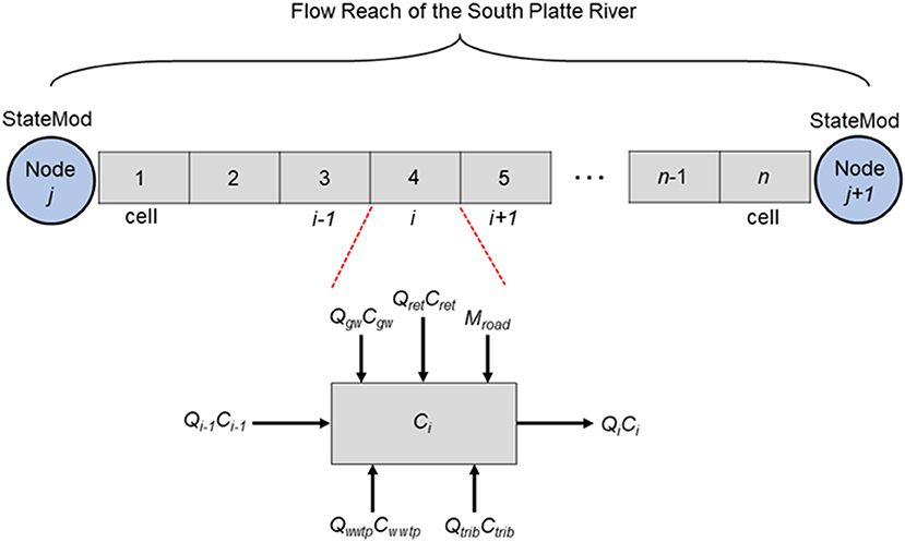
Figure 4. Schematic of the salt transport model of the South Platte River, showing n salt mass balance grid cells (control volumes) between two StateMod flow model nodes. Salt inputs and outputs for each grid cell can consist of groundwater discharge (gw), surface water return flows (ret), road salt (road), wastewater treatment plant effluent (wwtp), and tributary inflow (trib). Q, C, and M represent flow rates, concentrations, and mass, respectively.

South Platte River Upstream Concentration: the first StateMod node is the Highline Canal, located 160 km downstream of the South Platte River headwaters. Therefore, the section of the river before this canal is not modeled for flow or salinity. Based on sample data (NEIRBO, 2020), a salinity concentration value of 300 mg/L was assigned to this starting node.

Groundwater Concentration C_gw: Salinity concentration values of groundwater discharging to the river were estimated using measured TDS (mg/L) at groundwater monitoring wells in the basin (see Figure 5A for well locations and temporal averages). These data were obtained from the Colorado Agricultural Chemicals Groundwater Protection Water Quality Database (https://erams.com/co_groundwater/), a cooperation between the Colorado Department of Agriculture, Colorado State University Extension, and the Colorado Department of Public Health and Environment. The temporal average of TDS at each well during 1989–2018 was calculated and used in an Ordinary Kriging interpolation (spherical function) to provide basin-wide estimates of concentration (Figure 5B). Note that although the model simulation period is 2002–2006, we have used groundwater data from a longer date range due to the sparseness of groundwater salt ion data. We therefore assume that these concentrations are representative of those occurring during 2002–2006, due to the relatively slow movement of groundwater and groundwater fluxes. Concentration values from the interpolated map were then mapped to delineated subbasins (Figure 5C), and then to the river reach between two StateMod nodes, where they were assigned to the 100 m cells of the salt transport model. C_gw is assumed to be constant during the 2002–2006 simulation period. In the modeling approach, we assume that groundwater is not intercepted by irrigation canals, typical for this region.

FIGURE 5

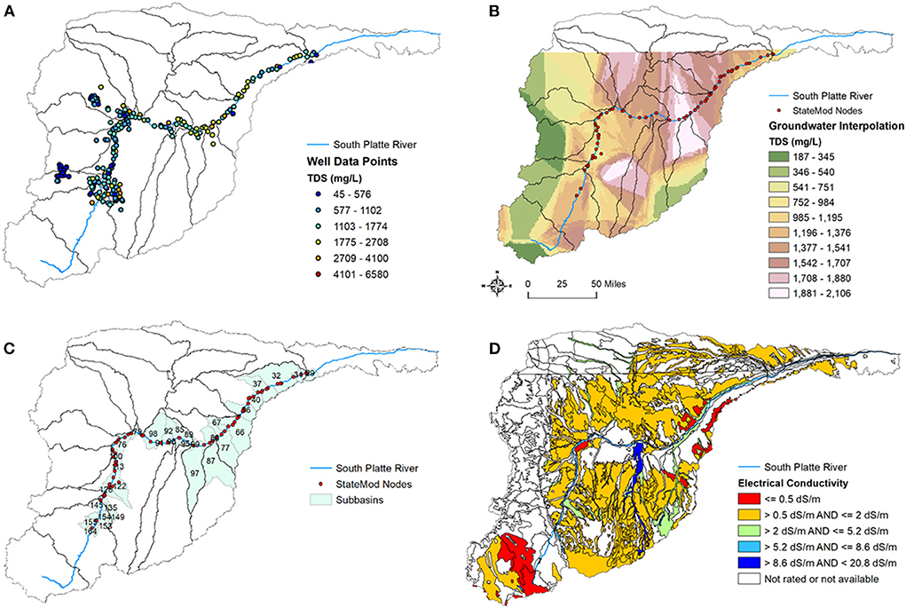
Figure 5. Maps showing sources and methods of salt inputs into the salt transport model for the South Platte River: (A) locations of groundwater monitoring wells and measured TDS (mg/L), (B) spatially interpolated TDS concentration from the well values, (C) subbasins along the South Platte River, and (D) soil electrical conductivity from NRCS soil maps.

Return Flow Concentrations C_ret: The concentration of salinity in surface water return flow is estimated using a combination of river water salinity concentration and soil salinity, as the salt mass in irrigation water runoff is a cominbation of salt mass in the diverted irrigation water (from the river) and the salt mass in the soil that dissolves into irrigation water during irrigation events. Soil salt concentration values were estimated using electrical conductivity (EC) (dS/m) values from STATSGO2 soil map data (Figure 5D) of the US Department of Agriculture, with the EC values converted to TDS using a conversion factor of 640 mg/L per dS/m (Northern Water, 2009). The soil TDS between a pair of StateMod nodes was calculated as the average value of the intersected subbasin values. The composite TDS concentration of return flow C_ret was calculated as the river's concentration at the upstream StateMod node, plus a percentage of the averaged soil concentration value between the upstream and downstream nodes. This percentage is referred to as the Return Flow % in the model.

Wastewater Treatment Plant Concentrations C_wwtp: Based on data from NEIRBO (2020), WWTP effluent salinity concentration was set to a constant value of 500 mg/L.

Tributary Concentrations C_trib: Daily EC values at the outlet sites of the three main tributaries (St. Vrain, Big Thompson, Cache la Poudre) were converted to average monthly values, and then converted to TDS concentration (mg/L).

Road Salt Concentration M_road: The amount of road salt applied was obtained from the Colorado Department of Transportation. The snow and ice material usage and chemical description for the Denver Metro area are provided in Supplementary Table 1. Products include calcium chloride (95% salt composition), salt-sand mix (11.5% salt), liquid deicer (28.5% salt), and salt brine (23.3% salt). The total amount of salt applied in the Denver Metro area was 63,100 tons, applied during winter months, with the same values used for each of the simulation period. This mass was converted to a mass rate (mass/time), of which 60% was assumed to return to the South Platte River within the Denver area.

Model simulations and testing

The integrated model was prepared and run in Excel using a variety of VBA scripts to simulate reach by reach stream discharge and salt concentration. The model was run for the period 2002–2006. Model results were tested against flow data at 14 gage sites (see Supplementary Figure 1 and Supplementary Table 2) and salt concentration data at 17 gage sites (see Supplementary Table 3). Three statistical measures are used to quantify the goodness-of-fit between observed and simulated flow and salt concentration: mean absolute error (MAE), the arithmetic average of the absolute error between predicted and observed data points; root mean squared error (RMSE), the residuals' standard deviation between predicted and observed data points; and Nash-Sutcliffe Coefficient of Efficiency (NSCE), a normalized statistic calculated as one minus the ratio of the modeled series' error variance divided by the observed series variance.

Sensitivity analysis

To quantify the influence of the driving forces of salt transport and loading in the South Platte River, the Morris sensitivity analysis method was implemented for the 2002–2006 period. For a model with K parameters, the elementary effect (EE) for parameter k with a deviation Δ was calculated as:

$\begin{array}{ll}E{E}_k=\frac{f(x_1,x_2,...,x_{k+\text{Δ}},x_K)-f(x_1,x_2,...,x_K)}{\text{Δ}}& (5)\end{array}$

The EEs are standardized by multiplying by the parameter value and dividing by the model output to calculate the standardized EE (SEE). For a model with K parameters, the SEE for parameter k with a deviation of Δ is calculated as:

$\begin{array}{ll}SE{E}_k=\frac{E{E}_k·x_{k+\text{Δ}}}{f(x_1,x_2,...,x_{k+\text{Δ}},x_K)}& (6)\end{array}$

The mean of the absolute value of the SEE values is calculated as μ^*, the parameter's overall sensitivity. The standard deviation of the SEE values is calculated as σ ^*, where σ ^* represents possible interaction effects between parameter k and other parameters and/or a non-linear effect on the model output. For parameter k with n_k number of EE, the σ ^* is calculated as:

$\begin{array}{ll}{{\sigma }^{*}}_k=\sqrt{\frac{1}{n_k}{\displaystyle \sum _{r=1}^{n_R}}{\left(\left|SE{E_k}^R\right|-{\mu }_k\right)}^2}& (7)\end{array}$

Two different sensitivity scenarios were studied. The first scenario was a spatial sensitivity study with the South Platte River split into five different reaches (see Supplementary Figure 2). The second scenario was a temporal sensitivity study performed over the entire South Platte River during the four seasons: spring, summer, fall, and winter. In both scenarios, 77 parameters were investigated for control on in-river salinity concentration. These parameters include initial upstream concentration, groundwater concentration for each reach, % of return flow that is from surface water in urban areas, % of return flow that is from surface water in agricultural areas, WWTP effluent flow rate and concentration, tributary flow rate and concentration (St. Vrain, Big Thompson, Cache la Poudre), and road salt mass loading. The list of parameters is provided in Supplementary Table 4. Each parameter was varied between ±10% of its baseline value.

Analysis of salt management practices

The controlling factors identified in the sensitivity analysis were used to design a suite of potential management practices to reduce salinity levels in the river. Two groups of scenarios were developed, one each for the upstream urban area and the downstream agricultural area. For the urban area, based on sensitivity analysis results (see Section Sensitivity analysis), management practices focused on road salt mass loading, initial upstream salt concentration in the river, the % of return flow that is surface water in urban areas, and the WWTP effluent concentration. For the agricultural area, management practices focused on road salt mass loading, the % of return flow that is surface water in urban areas, the % of return flow that is surface water in agricultural areas, and the WWTP effluent concentration.

For both scenarios, each parameter was assigned one of four value options: Baseline (no change), Low (5% reduction from baseline value), Medium (20% reduction), and High (35% reduction). 256 combinations of the targeted parameters and four value options were run for each month in the 2002–2006 period. Results are assessed for in-river salt concentration for the growing season (April to October) and the non-growing season (November to March) using a point system that calculates the decrease of in-river salt concentration reduction, as compared to the Baseline scenario, per unit of implemented reduction. Efficiency is determined by the decrease in river TDS (mg/L) per management practice points, with points totaled according to the level of implementation for each practice.

Results and discussion

Model results

Results of model testing are shown in Figures 6–8. Monthly flow model results are shown in Figure 6 for 4 months (March 2003, June 2003, August 2006, December 2004, to provide representative results from each season of the year), with the charts on the left showing flow rate per distance along the river for both simulated and measured (red dot) values, and the charts on the right showing 1:1 comparisons between simulated and measured values. NSCE values for each of the 60 months during the 2002–2006 simulation period are shown in Figure 7A. Fifty two of the 60 months have NSCE values between 0 and 1, with 35 months having a value above 0.5, indicating good model performance (Moriasi et al., 2015). Five of the 8 months that have NSCE < 0 occur in 2002, during which a major drought occurred, resulting in extremely low flow rates that are hard to match with the model. Overall, the model matches the spatial and temporal patterns of flow in the South Platte River. Referring to the spatial charts in Figure 6, the flow exhibits patterns of reservoir releases (inputs) and canal diversions (outputs). Flow rates in August 2006 are much lower than the other months, due to the cessation of snowmelt runoff.

FIGURE 6

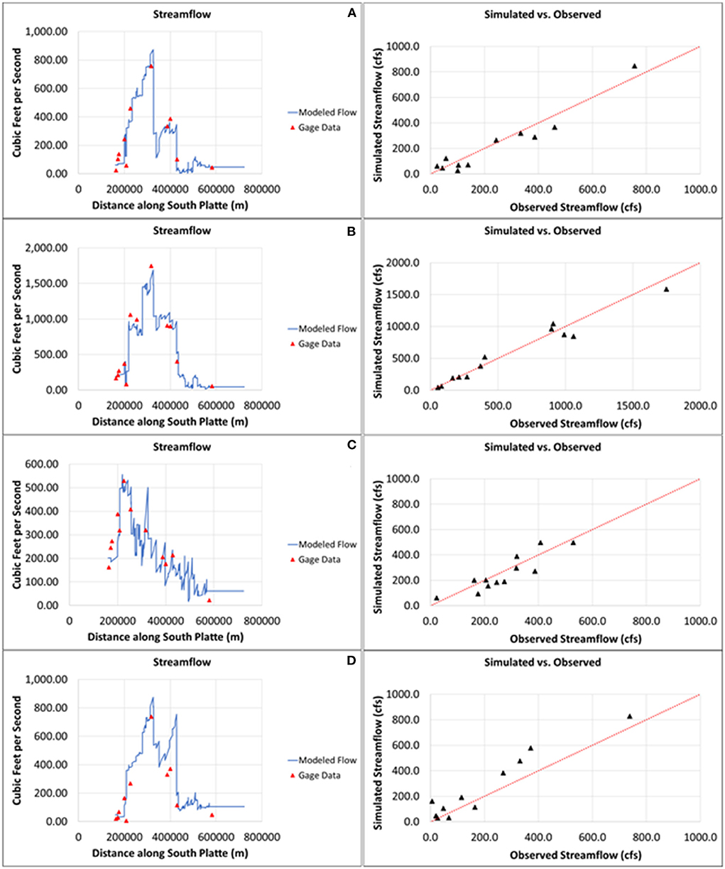
Figure 6. Flow model results for (A) March 2003, (B) June 2003, (C) August 2006, and (D) December 2004, showing flow rate at different locations in the river (charts on left) and 1:1 plots between observed and simulated flow rates (charts on right).

FIGURE 7

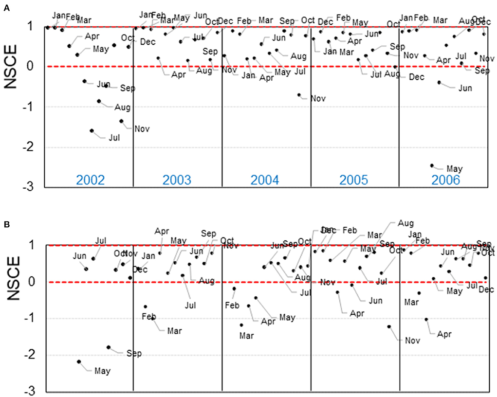
Figure 7. NSCE values for each month of the 2002–2006 period, for (A) flow rates in the South Platte River and (B) salt concentration values in the South Platte River. Monthly points are arranged chronologically, left to right.

FIGURE 8

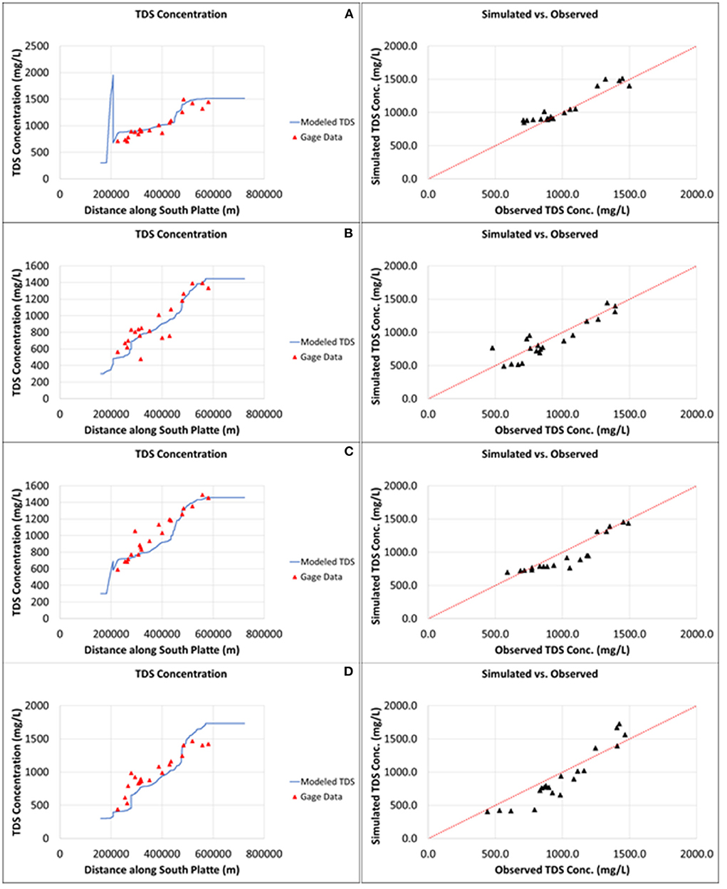
Figure 8. Salt model results for (A) January 2006, (B) September 2005, (C) November 2006, and (D) August 2006, showing salt concentration (mg/L) at different locations in the river (charts on left) and 1:1 plots between observed and simulated flow concentrations (charts on right).

Monthly salt concentration results are shown in Figure 8 for 4 months (January 2006, September 2005, November 2006, August 2006), with the charts on the left showing salt concentration per distance along the river for both simulated and measured (red dot) values, and the charts on the right showing 1:1 comparisons between simulated and measured values. Similar to the flow results, the salt transport model captures the spatial pattern of salt concentration, with values increasing downstream. Salt concentration with distance does not exhibit the same rises and falls of flow (see Figure 6), as loads and concentrations increase almost linearly downstream due to return flow of saline water into the river. Note the spike simulated concentration shown in Figure 8A (January 2006), a result of applied road salt in the Denver metro area. Interestingly, the simulated concentration decreases in the reaches just after the road salt input, coinciding with the measured values at the gages. Monthly NSCE values for the salt transport model are shown in Figure 7B. Although values are not as high as the flow model (also, 5 months have values below −3, not shown on the chart), 39 of the 60 months have values above 0, with 19 above 0.5. These results indicate the difficulty in representing accurately salt inputs in a large river basin. In addition, as salt concentration is directly affected by flow rates, any misrepresentation of flow rates (see Figure 7A) leads to poor representation of salt. However, due to the overall correct representation of spatial patterns of salt concentration and corresponding magnitudes, we conclude that the model can be used for analysis of management practice scenarios.

Sensitivity analysis

Sensitivity by river reach

Results of the spatial sensitivity analysis are shown in Figure 9. Only parameters with σ < 0.02 are shown graphically. Sensitivity indices for the urban area (Reach 2 in Supplementary Figure 2) are shown in Figure 9A, and indices for the agricultural area (Reach 5 in Supplementary Figure 2) are shown in Figure 9B. In the urban area, the salt concentration in the South Platte River is controlled principally by the WWTP effluent concentration (W Hite Concentration), and moderately by surface water return flow salinity (Return Flow % Before Union Ditch), the initial upstream concentration in the river (Initial Concentration), road salt mass loading (Road Salt), and the WWTP effluent flow rate (W Hite Flow). In the agricultural area, in-river salinity is controlled by surface return flow salinity in the agricultural area (i.e., after Union Ditch), the WWTP effluent concentration, concentration of tributary inflow water (St. Vrain, followed by Cache la Poudre and Big Thompson), groundwater concentration at Jud Brush Ditch (JUD BRUSH DITCH GW Conc), and road salt mass loading in the urban area. In general, except for the impact of surface return flow salinity, river salinity in the agricultural areas is governed by upstream salt inputs, either in the urban area (WWTP effluent, road salt) or tributary loads. Groundwater salinity has very little influence on in-river salinity.

FIGURE 9

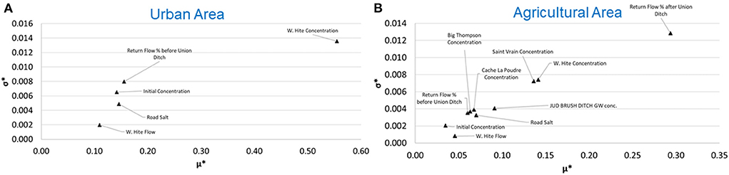
Figure 9. Results for the spatial (river reach) sensitivity analysis for the (A) urban area and the (B) agricultural area, showing the interaction effects σ^* plotted against the sensitivity index μ^* for salt model parameters.

Sensitivity by season

Results of the seasonal sensitivity analysis are shown in Figure 10. Similar to the spatial results shown in Figure 9, only parameters with σ < 0.02 are shown on the charts. Results can be summarized as follows for South Platte River salinity concentration:

FIGURE 10

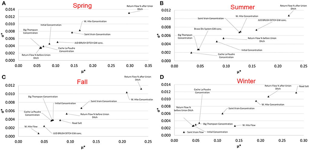
Figure 10. Results for the temporal (seasonal) sensitivity analysis for (A) spring months (March–May), (B) summer months (June–August), (C) fall months (September–November), and (D) winter months (December–February), showing the interaction effects σ^* plotted against the sensitivity index μ^* for salt model parameters.

Spring (March–May): governed by surface water return flow salinity, WWTP effluent concentration, St. Vrain inflow salt concentration, and groundwater concentration at Jud Brush Ditch.

Summer (June–August): same controls as during the spring months, except groundwater concentration at Jud Brush Ditch and the surface water return flow salinity in the urban area (i.e., before Union Ditch) have stronger influences.

Fall (September–November): same general results as spring and summer months, except with the inclusion of road salt mass as being impactful, likely due to snowstorms during the months of October and November.

Winter (December–February): same results as fall months, except road salt mass now has the strongest influence on in-river salinity. Also, WWTP effluent flow rate has a moderate influence.

In general, we conclude from these results that salt concentration in the South Platte River is largely governed by surface water return flow salinity, WWTP effluent concentration, and tributary inflow salt concentration, with road salt mass having a strong influence during the winter months. Surprisingly, due to the hydraulic connection between the aquifer and the river network in the basin, groundwater salt concentrations have little influence on in-river salinity. However, this may be due to the dissgregation of groundwater concentrations to specific river reaches (see Supplementary Table 4), with each reach having a small effect on in-river salinity.

Analysis of salt management practices

Urban reaches of the South Platte River

Based on sensitivity analysis results, the four targeted salt management practices for urban areas are treating WWTP effluent concentration, treating surface water return flow salinity in urban areas, treating concentration at the upstream point of the South Platte River, and decreasing road salt mass. Estimated results of implementing salt management practices in urban areas of the SPRB on in-river salinity in the urban reaches of the basin are shown in Figure 11A; Tables 1, 2. Tables 1, 2 show the most efficient practices for the months of April–October and November–March, respectively. There is one salt management point for each 5% of implementation. For example, the most efficient practice for the months of April–October (Table 1) is medium (20%) reduction in WWTP effluent concentration, which totals 4 points (1 point for each 5% implementation) and a decrease of 40 mg/L in the South Platte River (412 mg/L → 372 mg/L), resulting in an efficiency of 40 mg/L / 4 points = 10 mg/L per point. The high reduction (35% = 7 points) resulted in a decrease of 70 mg/L, and therefore also an efficiency of 10 mg/L per point.

FIGURE 11

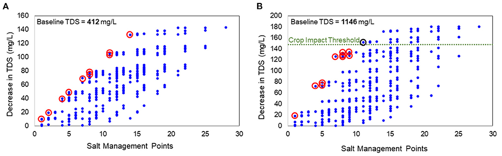
Figure 11. Results of the salt management strategies for (A) the urban areas and the (B) agricultural areas, for the months April–October. Each blue dot represents a unique strategy, with the red circles indicating the 10 most efficient strategies, based on the ratio of the decrease in TDS from the baseline value to salt management points. In (B), the crop impact threshold, which corresponds to an in-river concentration of 1,000 mg/L (146 decrease from the 1,146 mg/L baseline value), is shown in a green dotted line. The black circle indicates the most efficient salt management strategy that meets the crop impact threshold of 1,000 mg/L.

TABLE 1

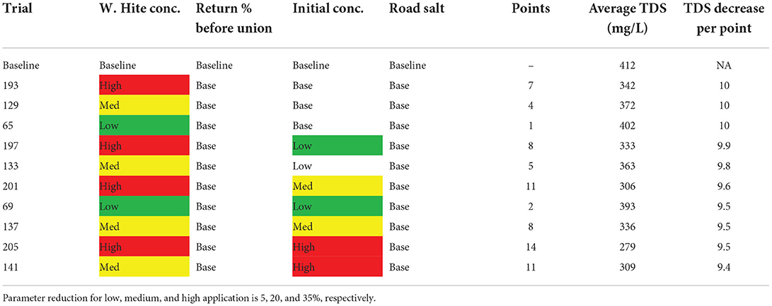
Table 1. Top 10 efficient urban salt management trials for the months April–October.

TABLE 2

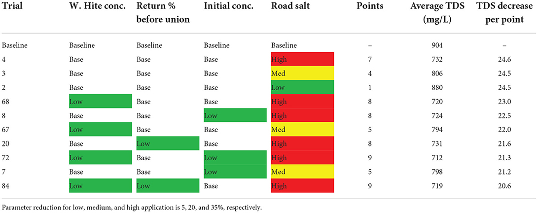
Table 2. Top 10 efficient urban salt management trials for the months November–March.

Results for all 256 salt management practice combinations for the months April–October are shown in Figure 11A, with the decrease in TDS (mg/L) in the urban reach of the South Platte River for each practice plotted against the salt management points. Each blue dot represents a unique practice or combination of practices. The circled dots represent the 10 most efficient practices, listed in Table 1. Notice that these practices fall along the left-most edge of the scatter plot, indicating the largest decrease in TDS for the fewest management points (i.e., the smallest intervention). Efficiency, however, does not necessarily indicate a strong response in the river, as indicated by several of the “efficient” practices in Figure 11A that produce a decrease of only 10–50 mg/L in the South Platte River.

In addition, the spatial patterns shown in Figure 11A demonstrate a point of diminishing returns, with an increase in salt management points (>15) not providing any additional decrease in TDS (~140 mg/L). Therefore, trial 205 (35% reduction in WWTP effluent concentration, 35% reduction in upstream salt concentration) (see Table 1 and the farthest-right efficient practice in Figure 11A) can represent the optimal practice in terms of providing the highest decrease in TDS for the lowest degree of salt management practice implementation. Of course, we recognize that in all these results, ease of implementation and economic cost of targeted salt management practices are not considered, and that a percentage decrease for one practice is not necessarily equivalent to a percentage decrease in another practice. This study provides a basis for understanding which practices can be effective at decreasing salt concentration; additional studies are needed to quantify cost and overall feasibility.

Agricultural reaches of the South Platte River

Based on sensitivity analysis results, the four targeted salt management practices for urban areas are treating WWTP effluent concentration, treating surface water return flow salinity in urban areas, treating surface water return flow salinity in agricultural areas, and decreasing road salt mass. Estimated results of implementing salt management practices in agricultural areas of the SPRB on the in-river TDS at the Colorado-Nebraska border are shown in Figure 11B; Tables 3, 4. Tables 3, 4 show the most efficient practices for the months of April–October and November–March, respectively. For April–October, the most efficient practice is an aggressive (35%) reduction in surface water return flow salinity, which results in a decrease of 126 mg/L (1,146 mg/L → 1,020 mg/L) in the South Platte River. Most of the top 10 efficient practices include a focus on return flow salinity, with low (5%) reductions in the other three practices. Similar results are obtained for November–May (Table 4), with return flow being the most impactful practice.

TABLE 3

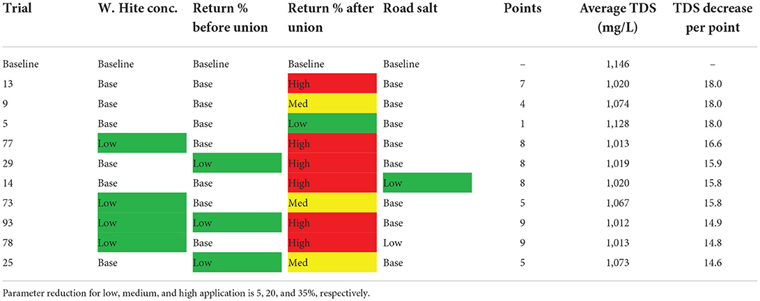
Table 3. Top 10 efficient agricultural salt management trials for the months April–October.

TABLE 4

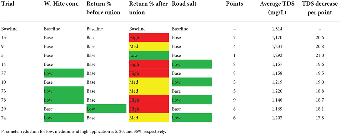
Table 4. Top 10 efficient agricultural salt management trials for the months November–March.

Figure 11B shows Results for all 256 salt management practice combinations for the months April–October. The largest decrease in TDS is 181 mg/L, resulting in an in-river concentration of 965 mg/L. Similar to the urban area results (Figure 11A), the 10 most efficient practices are circuled in red. The chart also shows the “Crop Impact Threshold” which indicates the decrease in TDS (mg/L) (146 mg/L) from the baseline value of 1,146 mg/L that must occur to achieve the target concentration of 1,000 mg/L, corresponding to river water that likely will not result in crop yield reduction if diverted and applied as irrigation water. We note that none of the 10 practices listed in Table 3, although “efficient” in regards to the decrease in TDS per management practice points, achieve the salinity target of 1,000 mg/L in the South Platte River. Therefore, aggressive strategies are required if this target is to be achieved. Of the 256 practice combinations assessed in this study, 32 (12.5%) achieve the salinity target (i.e., decrease of more than 146 mg/L, being above the crop impact threshold in the chart). Of these 32 practices, the most efficient practice (circuled in black in Figure 11B) is a combination of high (35%) reduction of return flow salinity and medium (20%) reduction of WWTP effluent concentration, resulting in a river concentration of 994 mg/L.

Summary and conclusions

This study uses an integrated one-dimensional hydro-salinity river flow and transport model to investigate controlling factors of river salinity in the South Platte River and quantify effects of implementing salt management practices on in-river salt concentration (mg/L). The South Platte River (563 km) flows through urban areas (Front Range of the Rocky Mountains in Colorado and Wyoming) and into agricultural areas, where river water is used extensively for irrigation. The model consists of a water allocation and streamflow model (StateMod) provided by the Colorado Division of Water Resources and a salt transport model developed for this study. The water allocation model accounts for all water transfers (e.g., reservoir releases, canal diversion, return flows from surface water and groundwater) along the highly-managed South Platte River, and the salt transport model accounts for all major salt sources and sinks: groundwater loading, surface water return flow loading, wastewater treatment plant (WWTP) effluent loading, tributary loading, and road salt loading, with the latter occurring in the urban areas, particularly in the Denver metro area. The model is tested against stream discharge and in-river salt concentration at a network of gage sites for the period 2002–2006, and then used in sensitivity analysis and scenario analysis. This is a unique study that investigates the movement of salt in a large agro-urban river basin, and the possible mitigation schemes that can be implemented in both urban and agricultural areas to improve river water quality. This is particularly important for downstream agricultural regions that rely on river water for crop water needs.

Results from the sensitivity analysis indicate the following:

• River salinity in urban areas is controlled principally by effluent loading from a major WWTP in the Denver area. Surface water return flow salinity, upstream river salt concentration, and road salt loading all had similar effects on river salinity. As expected, road salt has a stronger influence during the winter months (December–February).

• River salinity in agricultural areas (downstream of the urban areas) is controlled principally by surface water return flow salinity (i.e., irrigation runoff), followed by WWTP effluent concentration from the Denver area, tributary salt loading into the river, groundwater salinity loading, and road salt loading in the urban areas. As expected, road salt has a stronger influence during the winter months (December–February).

• Although the South Platte River is in strong hydraulic connection with the alluvial aquifer system, and irrigation practices tend to increase groundwater levels thereby inducing groundwater return flow to the river, groundwater salinity loading to the river does not have a strong impact on in-river salinity concentration. Only one small section of the river exhibited an influence of groundwater salinity that was similar in effect to other salt inputs.

Results from the analysis of salt management scenarios indicate the following:

• Efficient practices (i.e., large decrease in river salt concentration compared to implementation level of salt management practices) in urban areas during the spring and summer months focus mainly on WWTP effluent concentration (35% reduction) in the Denver metro area and treating upstream river water (i.e., water treatment plants), resulting in concentration decreases of 70–120 mg/L (15–30% decrease from baseline) in the urban reaches of the South Platte River. During winter months, the most efficient practices include medium (20%) and high (35%) reduction in road salt. These practices results in concentration decreases of 100–200 mg/L (10–20% decrease from baseline).

• Efficient practices in agricultural areas during both spring/summer months and fall/winter months focus on surface water return flow salinity (5–35% reduction) and low (5% reduction) treatment of WWTP effluent concentration and road salt, resulting in concentration decreases of 70–135 mg/L (5–12% decrease from baseline). During winter months, the most efficient practices include medium (20%) and high (35%) reduction in road salt. These practices results in concentration decreases of 80–170 mg/L (5–13% decrease from baseline).

• Of the 256 salt management practice combinations investigated, only 32 achieve the salinity target of 1,000 mg/L in the South Platte River, which is targeted for minimal impact on crop growth and yield when diverted and used as irrigation water. These 32 practices are extremely aggressive, with the most efficient including a combination of high (35%) reduction of surface water return flow salinity and medium (20%) reduction of WWTP effluent concentration, which in our estimates would result in a river concentration of 994 mg/L. Even with implementing high levels of implementation (35% reduction) in WWTP effluent concentration, surface water return flow salinity, and road salt, the lowest achieved concentration is 965 mg/L, near the 1,000 mg/L threshold. These results point to the immediate and difficult challenge of controlling salt levels in rivers of agro-urban river basins, particularly those with upstream urban areas.

This study highlights the interplay between urban areas and agricultural areas in determining salt concentrations in a large agro-urban river basin, and the immense challenge of decreasing salt concentration levels to appropriate levels for crop irrigation. Downstream agricultural areas are largely dependent on urban areas to control salt loadings (WWTP effluent, road salt) into the river system. Surface water return flow salinity has a strong effect on river water salinity in these areas; however, the salt content of the return flows is a product of the salt concentration in diverted river water, which is controlled by upstream urban activities. The method presented in this paper can be used in other large river basins to investigate salt movement and possible remediation strategies. Overall, findings from this study can be applicable to other semi-arid agro-urban river systems that exhibit high in-river salt concentration.

Data availability statement

The original contributions presented in the study are included in the article/Supplementary material, further inquiries can be directed to the corresponding author/s.

Author contributions

RB planned the research, provided the funding, oversaw the results and analysis, and wrote the main draft of the paper. CH performed the research details, wrote code for running the model, developed management scenarios, and performed the analysis. Both authors contributed to the article and approved the submitted version.

Funding

Financial support for this study was provided by National Science Foundation, Award No. 1845605.

Conflict of interest

The authors declare that the research was conducted in the absence of any commercial or financial relationships that could be construed as a potential conflict of interest.

Publisher's note

All claims expressed in this article are solely those of the authors and do not necessarily represent those of their affiliated organizations, or those of the publisher, the editors and the reviewers. Any product that may be evaluated in this article, or claim that may be made by its manufacturer, is not guaranteed or endorsed by the publisher.

Supplementary material

The Supplementary Material for this article can be found online at: https://www.frontiersin.org/articles/10.3389/frwa.2022.945682/full#supplementary-material

References

Aliyari, F., Bailey, R. T., Tasdighi, A., Dozier, A., Arabi, M., and Zeiler, K. (2019). Coupled SWAT-MODFLOW model for large-scale mixed agro-urban river basins. Environm. Model. Softw. 115, 200–210. doi: 10.1016/j.envsoft.2019.02.014

CrossRef Full Text | Google Scholar

Arnold, J. G., Srinivasan, R., Muttiah, R. S., and Williams, J. R. (1998). Large area hydrologic modeling and assessment part I: model development 1. JAWRA J. Am. Water Resour. Assoc. 34, 73–89. doi: 10.1111/j.1752-1688.1998.tb05961.x

CrossRef Full Text | Google Scholar

Asensio, E., Ferreira, V. J., Gil, G., García-Armingol, T., López-Sabirón, A. M., and Ferreira, G. (2017). Accumulation of de-icing salt and leaching in Spanish soils surrounding roadways. Int. J. Environ. Res. Public Health 14, 1498. doi: 10.3390/ijerph14121498

PubMed Abstract | CrossRef Full Text | Google Scholar

Bailey, R. T., Tavakoli-Kivi, S., and Wei, X. (2019). A salinity module for SWAT to simulate salt ion fate and transport at the watershed scale. Hydrol. Earth Syst. Sci. 23, 3155–3174. doi: 10.5194/hess-23-3155-2019

CrossRef Full Text | Google Scholar

Burkhalter, J. P., and Gates, T. K. (2006). Evaluating regional solutions to salinization and waterlogging in an irrigated river valley. J. Irrig. Drainage Eng. 132, 21–30. doi: 10.1061/(ASCE)0733-9437(2006)132:1(21)

CrossRef Full Text | Google Scholar

Cañedo-Argüelles, M., Kefford, B. J., Piscart, C., Prat, N., Schäfer, R. B., and Schulz, C. J. (2013). Salinisation of rivers: an urgent ecological issue. Environ. Pollut. 173, 157–167. doi: 10.1016/j.envpol.2012.10.011

PubMed Abstract | CrossRef Full Text | Google Scholar

Cook, M. (2015). South Platte Basin Implementation Plan. Technical Report. West Sage Water Consultants.

Google Scholar

Dennehy, K. F. (1998). Water Quality in the South Platte River Basin, Colorado, Nebraska, and Wyoming. 1992-95 (Vol. 1167). US Department of the Interior, US Geological Survey.

Google Scholar

Dietz, M. E., Angel, D. R., Robbins, G. A., and McNaboe, L. A. (2017). Permeable asphalt: a new tool to reduce road salt contamination of groundwater in urban areas. Groundwater 55, 237–243. doi: 10.1111/gwat.12454

PubMed Abstract | CrossRef Full Text | Google Scholar

Dugan, H. A., Bartlett, S. L., Burke, S. M., Doubek, J. P., Krivak-Tetley, F. E., Skaff, N. K., et al. (2017). Salting our freshwater lakes. Proc. Natl. Acad. Sci. 114, 4453–4458. doi: 10.1073/pnas.1620211114

PubMed Abstract | CrossRef Full Text | Google Scholar

Haby, P. A., and Loftis, J. C. (2000) Salinity characterization source assessment in the South Platte River Basin, northeastern Colorado. Watershed Manag. Oper. Manag. 2000, 1–7. 10.1061/40499(2000)132

Google Scholar

Hassani, A., Azapagic, A., and Shokri, N. (2020). Predicting long-term dynamics of soil salinity and sodicity on a global scale. Proc. Natl. Acad. Sci. 117, 33017–33027. doi: 10.1073/pnas.2013771117

PubMed Abstract | CrossRef Full Text | Google Scholar

Huang, W., and Foo, S. (2002). Neural network modeling of salinity variation in Apalachicola River. Water Res. 36, 356–362. doi: 10.1016/S0043-1354(01)00195-6

PubMed Abstract | CrossRef Full Text | Google Scholar

Hunter, J. M., Maier, H. R., Gibbs, M. S., Foale, E. R., Grosvenor, N. A., Harders, N. P., et al. (2018). Framework for developing hybrid process-driven, artificial neural network and regression models for salinity prediction in river systems. Hydrol. Earth Syst. Sci. 22, 2987–3006. doi: 10.5194/hess-22-2987-2018

CrossRef Full Text | Google Scholar

Jung, C., Ahn, S., Sheng, Z., Ayana, E. K., Srinivasan, R., and Yeganantham, D. (2021). Evaluate river water salinity in a semi-arid agricultural watershed by coupling ensemble machine learning technique with SWAT model. JAWRA J. Am. Water Res. Assoc. 1–14. doi: 10.1111/1752-1688.12958

CrossRef Full Text | Google Scholar

Lee, D. J., Howitt, R. E., and Mariño, M. A. (1993). A stochastic model of river water quality: application to salinity in the Colorado River. Water Res. Res. 29, 3917–3923. doi: 10.1029/93WR02464

CrossRef Full Text | Google Scholar

Maleki, M. S., Banihabib, M. E., and Randhir, T. O. (2021). SWAT-SF: a flexible SWAT-based model for watershed-scale water and soil salinity modeling. J. Contaminant Hydrol. 244, 103893. doi: 10.1016/j.jconhyd.2021.103893

PubMed Abstract | CrossRef Full Text | Google Scholar

Meyer, E. S., Sheer, D. P., Rush, P. V., Vogel, R. M., and Billian, H. E. (2020). Need for process based empirical models for water quality management: salinity management in the Delaware river basin. J. Water Resour. Plann. Manag. 146, 05020018. doi: 10.1061/(ASCE)WR.1943-5452.0001260

CrossRef Full Text | Google Scholar

Moriasi, D. N., Gitau, M. W., Pai, N., and Daggupati, P. (2015). Hydrologic and water quality models: performance measures and evaluation criteria. Transac. ASABE. 58, 1763–1785. doi: 10.13031/trans.58.10715

CrossRef Full Text | Google Scholar

NEIRBO. (2020). South Platte River Salinity. Available online at: https://www.neirbo.com/

Google Scholar

Northern Water (2005). A Study of Salinity in the Lower South Platte Basin. Available online at: https://www.northernwater.org/what-we-do/protect-the-environment/reports

Google Scholar

Northern Water (2009). A Study of Salinity in the Lower South Platte Basin. Available online at: https://www.northernwater.org/what-we-do/protect-the-environment/reports

Google Scholar

Novotny, E. V., Murphy, D., and Stefan, H. G. (2008). Increase of urban lake salinity by road deicing salt. Sci. Tot. Environ. 406, 131–144. doi: 10.1016/j.scitotenv.2008.07.037

PubMed Abstract | CrossRef Full Text | Google Scholar

Novotny, E. V., and Stefan, H. G. (2010). Projections of chloride concentrations in urban lakes receiving road de-icing salt. Water Air Soil Pollut. 211, 261–271. doi: 10.1007/s11270-009-0297-0

CrossRef Full Text | Google Scholar

Olson, J. R. (2019). Predicting combined effects of land use and climate change on river and stream salinity. Philos. Trans. R. Soc. B 374, 20180005. doi: 10.1098/rstb.2018.0005

PubMed Abstract | CrossRef Full Text | Google Scholar

Sadoddin, A., Letcher, R. A., Jakeman, A. J., and Newham, L. T. (2005). A Bayesian decision network approach for assessing the ecological impacts of salinity management. Math. Comput. Simul. 69, 162–176. doi: 10.1016/j.matcom.2005.02.020

CrossRef Full Text | Google Scholar

Singh, A., and Panda, S. N. (2012). Integrated salt and water balance modeling for the management of waterlogging and salinization. I: validation of SAHYSMOD. J. Irrig. Drain. Eng. 138, 955–963. doi: 10.1061/(ASCE)IR.1943-4774.0000511

CrossRef Full Text | Google Scholar

Tedeschi, A., Beltran, A., and Aragüés, R. (2001). Irrigation management and hydrosalinity balance in a semi-arid area of the middle Ebro river basin (Spain). Agric. Water Manag. 49, 31–50. doi: 10.1016/S0378-3774(00)00117-7

CrossRef Full Text | Google Scholar

Thorslund, J., and van Vliet, M. T. (2020). A global dataset of surface water and groundwater salinity measurements from 1980–2019. Sci. Data 7, 1–11. doi: 10.1038/s41597-020-0562-z

PubMed Abstract | CrossRef Full Text | Google Scholar

Tirabadi, M.S. M., Banihabib, M. E., and Randhir, T. O. (2021). SWAT-S: a SWAT-salinity module for watershed-scale modeling of natural salinity. Environ. Model. Softw. 135, 104906. doi: 10.1016/j.envsoft.2020.104906

CrossRef Full Text | Google Scholar

Trenouth, W. R., Gharabaghi, B., and Perera, N. (2015). Road salt application planning tool for winter de-icing operations. J. Hydrol. 524, 401–410. doi: 10.1016/j.jhydrol.2015.03.004

CrossRef Full Text | Google Scholar

Tuteja, N. K., Beale, G., Dawes, W., Vaze, J., Murphy, B., Barnett, P., et al. (2003). Predicting the effects of landuse change on water and salt balance—a case study of a catchment affected by dryland salinity in NSW, Australia. J. Hydrol. 283, 67–90. doi: 10.1016/S0022-1694(03)00236-1

CrossRef Full Text | Google Scholar

Williams, W. D. (1999). Salinisation: a major threat to water resources in the arid and semi-arid regions of the world. Lakes Reserv. Res. Manag. 4, 85–91. doi: 10.1046/j.1440-1770.1999.00089.x

CrossRef Full Text | Google Scholar