 David Dziubanski†
 Kristie J. Franz*†
- Department of Geological and Atmospheric Sciences, Iowa State University, Ames, IA, United States
Watershed systems are changing due to human activities within the landscape and shifting precipitation patterns, and quantifying the coupled effects of these two factors is necessary for anticipating future hydrologic response. In this study, we use a model that combines an agent-based model (ABM) with a semi-distributed hydrologic model to assess how projected changes in precipitation and temperature affect streamflow when simultaneously considering how those variables impact the land use decisions that also influence watershed response. We use a flood-prone watershed which is characteristic of many agriculturally-dominated watersheds in the central Midwest US. In the ABM, farmer agents make decisions that affect land use based on factors related to profits, past land use, neighbor influence, and internal behavior. A city agent aims to reduce urban flooding by paying farmer agents a subsidy for allocating land to conservation practices that reduce runoff. We run the model for the 2018–2097 period using the Representative Concentration Pathway (RCP) 4.5 and RCP 8.5 climate scenarios and different decision-making options. The model reveals that under future precipitation, which becomes increasingly intense leading to more in-field flooding, farmers increase conservation land by up to 60%. This land conversion results in a 4–7% decrease in mean 95th percentile discharge relative to scenarios where conservation land is held constant at the historical mean. If farmers are allowed to modify their internal behavior and preferences, the mean 95th percentile discharge decreases further (up to 16%). Using the assumption that land owners are willing to adapt their personal preferences to mitigate the negative effects of climate change on their land and external incentives exist to do so, upstream runoff mitigation practices could reduce downstream impacts from more frequent intense precipitation. However, farmer agents converted, on average, <10% of their land to conservation even when this variable was unrestricted. By the end of the century, precipitation has the dominant influence on discharge, given the significant changes in projected precipitation and the limited land conversion.
1. Introduction
The hydrology of many river basins across the world is continually changing due to a combination of climate change and human interventions (Christensen et al., 2004; Naik and Jay, 2011; Steffens and Franz, 2012; Frans et al., 2013). In 2008, Milly et al. argued that increasing anthropogenic change of Earth's climate is altering precipitation patterns, which is in turn affecting runoff (Milly et al., 2008). However, human alterations of the natural hydrologic system, such as river channel modification, urbanization, and agricultural practices, are also changing watershed behavior (Turner and Rabalais, 2003; Cruise et al., 2010; Carpenter et al., 2011; Chelsea Nagy et al., 2012; Sivapalan et al., 2012; Montanari et al., 2013). Understanding the respective impact of climate change vs. human practices, and their combined effect, remains a challenge because of the difficulty of projecting the dynamic behavior of each system into the future.
Precipitation extremes are increasing across the United States, and are expected to further increase under future climate (Kunkel et al., 1999; Gutowski et al., 2007; Karl et al., 2009; Groisman et al., 2012; Zhang et al., 2013; Wuebbles et al., 2014; Prein et al., 2017). Villarini et al. (2013) studied precipitation trends across the Central U.S. using data from 447 rain gauges located in a region stretching from Minnesota to Louisiana. They found a statistically significant increasing trend in the frequency of heavy rainfall events for 90 stations, particularly over northern states, with three stations showing a decreasing trend. In turn, the changing precipitation patterns are leading to changes in flooding. One study found that 34% of 774 stream gaging stations in the central US recorded an increased frequency of flood events over the last 50 years or more (Mallakpour and Villarini, 2015). Only 9% of stations showed a decreasing frequency. With the increased frequency of extreme precipitation expected to continue (Janssen et al., 2014; Wuebbles et al., 2014; Karmalkar and Bradley, 2017; Prein et al., 2017), so too will the potential for flood risk in many regions of the U.S. (Milly et al., 2002; Arnell and Gosling, 2016; Naz et al., 2016).
Since hydrologic changes arise from both climate and human factors, a number of recent hydrologic studies have placed importance on trying to decipher the relative contributions of these factors on changes in river discharge (Tomer and Schilling, 2009; Wang and Cai, 2010; Naik and Jay, 2011; Frans et al., 2013; Ye et al., 2013; Ahn and Merwade, 2014). These studies use a variety of techniques, such as modeling and statistical methods (e.g., linear regression), water balance approaches, trend analysis, and Budyko analysis and have shown that a significant percentage of the recent changes in streamflow can be attributed to human-induced changes. For instance, Ahn and Merwade (2014) found significant human impacts to streamflow at 85% of stations in Georgia. Schilling et al. (2010) determined that ~30% of the increase in water flux observed in the Mississippi river basin over the last 100 years can be attributed to dramatic increases in soybean acreage since 1940. On the other hand, Frans et al. (2013) found climate to be a dominating factor (>90%) in runoff change in the Upper Mississippi River Basin. Despite variations in the amount of hydrologic change attributable to land use, these and other studies (O'Keeffe et al., 2018; Kwak and Deal, 2021; Ross and Chang, 2021) make clear that both climate and human factors need to be considered when evaluating climate mitigation and water management strategies.
In this study, we use the agent-based hydrologic model of Dziubanski et al. (2020) to assess how changes in precipitation and temperature affect streamflow when simultaneously considering how those variables impact the land use decisions that also influence watershed response. We use the same representative watershed of Dziubanski et al. (2020), which is characteristic of flood-prone, agriculturally-dominated watersheds in the central Midwest US. Five climate simulations of temperature and precipitation for the 2018–2097 period from the North American CORDEX program (Mearns et al., 2017) are used to drive the model under two primary climate scenarios: representative concentration pathways (RCP) 4.5 and RCP 8.5 (Van Vuuren et al., 2011). Social-hydrologic models, such as the Dziubanski et al. (2020) model, allow the natural and social systems to co-evolve within one computational framework (Sivapalan et al., 2012; Montanari et al., 2013) allowing the model user to control and observe the impact of external and internal factors on system outcomes. Taking advantage of the capabilities of agent-based modeling, we run the model under the climate scenarios using the following decision-making scenarios: (1) farmer agents are allowed to change land use to/from conservation through time, but their decision behavior remains stationary, (2) farmer agent are allowed to change land use through time and their decision behavior may change through time, and (3) land use remains unchanged at the historical mean throughout the simulation. The model output is used to explore the following research questions:
1) How might farmers in a Midwestern US landscape change land use practices in response to future climate, assuming current agro-economic conditions and incentive programs?
2) What are the combined and individual impacts of human activities and climate on changes in streamflow?
2. Materials and methods
The modeling system is comprised of natural system models that produce annual peak streamflow, in-field flooding, and crop yield, and an agent-based model (ABM) of agricultural and urban decision-making (Figure 1). The ABM includes two primary agents (farmer and city) that interact through conservation contracts in which the city pays the farmer to implement conservation practices that reduce runoff and flooding. Farmer agent attributes and farm land characteristics vary stochastically throughout the watershed, which when combined with climate conditions, make the human impact component uncertain and unpredictable both spatially and temporally. The agent (social) and natural systems within the model dynamically interact and influence the external climate and economic (government and market) systems (Figure 1). Model details and validation can be found in Dziubanski et al. (2020). This methods section provides an overview of key model components and describes functions that have been added since the prior study.

Figure 1. Flowchart of the socio-hydrologic model.
2.1. Economic system
The market module provides information about forecasted and realized crop prices and production costs that agents use in their decision making. Crop price projections for 10 years into the future are calculated annually based on historical crop prices and error estimates of U.S Department of Agriculture (USDA) crop price forecasts. The 10-year forecast is developed using the following equation (Dziubanski et al., 2020):
where CropPriceForecastt+n is the forecasted crop price for year t + n (t is the current year, 1 ≤ n ≤ 10), CropPricet+n is the historical crop price for year t+n, ErrorCropPrice is the error based on CropPricet+n. Twelve years of USDA crop price forecasts for 2001–2012 were analyzed against realized crop prices to form the error functions used in the market module:
where A, B, and C are coefficients from the regression. There are 12 error equations in the market module, and the error equation with a starting crop price closest to the current year's crop price is used to formulate the 10-year forecast. The market module also annually calculates production costs taking into consideration variability in crop insurance costs as a function of past yields, and land rental rates based on crop prices.
2.2. Social system
2.2.1. Farmer agent module
The farmer agent is characterized by two primary state variables, “conservation mindedness” and risk aversion attitude (McGuire et al., 2013; Prokopy et al., 2019). “Conservation mindedness” is represented through a conservation parameter (Consmax), which indicates the degree to which the farmer agent is willing to adopt on-farm conservation practices, a concept presented by McGuire et al. (2013). Consmax represents the maximum fraction of land a farmer is willing to put into conservation and ranges from 0.0 to 0.1, or 0 to 10% of the farmer's land (Table 1). The maximum value of 10% is based on the runoff reduction practice available to farmer agents in this model, in which 10% of the total farm plot area is converted to prairie vegetation planted in strips (e.g., native prairie strips) perpendicular to the primary flow direction within the farm plot (Helmers et al., 2012; Hernandez-Santana et al., 2013; Zhou et al., 2014). The secondary state variable is risk-aversion, which describes the willingness of the farmer agent to change land use under uncertainty (Prokopy et al., 2019). High risk averse farmers are more likely to maintain the same land use, even as crop prices decline. In addition to conservation mindedness and risk aversion, farmer agents' decisions are modified by future crop price projections, past profits, and neighbor decisions.
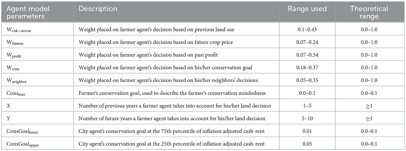
Table 1. Primary agent model parameters in decision-making equations.
A farmer agent decides how much land to allocate into conservation, Dt, for the current year t based on the following equation (Dziubanski et al., 2020):
where Ct−1:t−X is the mean total amount of land allocated to conservation during the previous X years, Dt−1 is the prior conservation decision (total amount of land the farmer would have liked to implement in conservation) in year t − 1, δCfutures:Y is the decision based on crop price projections for Y years into the future, δCprofit:X is the decision based on the mean past profit of the previous X years, δCcons is the decision based on the conservation goal of the farmer, and Cneighbor is the weighted mean conservation land of the farmer agent's neighbors (Table 1). Parameters X and Y represent the number of prior or future years the farmer agent considers in the decision making. Decision weights (Table 1) alter how each of the five components factor into a farmer agent's decision and are assigned individually to a farmer agent such that:
The decision components for past profit and future crop prices are based on a partial budgeting approach, which takes into account added and reduced income and added and reduced costs from a particular land conversion (Tigner, 2006). The budget calculation indicates the net gain or loss in income that a farmer agent may incur from changing an acre of land to/from crop production or conservation (Dziubanski et al., 2020). Yields, production costs, federal subsidies, crop insurance, and the cost to establish and maintain conservation land are considered. In addition, farmer agent's land is randomly assigned varied soil types, which influence crop productivity, crop production costs, and opportunity costs. Thus, farmers convert less profitable land to conservation first.
The past profits decision is based on outcomes that have been fully realized for the previous X years and the amount of money that could have been earned per hectare of conservation land vs. crop land. The future crop prices decision is based on a combination of past performance information and projected future crop prices. δCprofit and δCfutures can take on values between −100% and 100% depending upon whether the farmer agent expects a higher revenue from crops or conservation land. The methods used to calculate δCprofit:X and δCfutures:Y are described in detail in Dziubanski (2018) and Dziubanski et al. (2020).
The conservation goal (δCcons) decision is defined by the Bernoulli distribution where the probability p of fully implementing conservation land is a function of the agent's Consmax parameter and is computed by (Dziubanski et al., 2020):
The probability p scales from 0 at a Consmax of 0, to 1 at a Consmax of 0.1 such that, a farmer agent with a Consmax of 0.05 will have a 50% probability of fully implementing conservation land in any given year based on their conservation decision.
The diffusion of conservation adoption due to the influence of interpersonal interactions (Saltiel et al., 1994; Davis and Gillespie, 2007; Arbuckle et al., 2013; McGuire et al., 2013) is represented by a probabilistic-based network that determines the value of Cneighbor (Dziubanski et al., 2020). Agents connect only within their subbasin. Each agent in a subbasin of n agents can make up to n − 1 connections, where the number of connections that an agent makes is randomly drawn from a binomial distribution (Newman et al., 2002). Currently in the model, each possible connection is set to have the same success probability of p = 0.5, indicating a 50% probability of forming a connection with any one farmer. Once a farmer agent initiates a connection with another farmer agent, they are both assigned a ConnStrength value that is randomly chosen from the uniform distribution: . The probability that a farmer agent will exchange land use information with the other farmer agent during any given year is described by the Bernoulli distribution with p = ConnStrength (Granovetter, 1973). If the choice of connection is a success for both farmer agents (i.e., both farmer agents “draw” a 1), they share information; however, if the choice of connection is a success for only one farmer agent, then the agents do not share information.
2.2.2. City agent module
The city agent is defined by a conservation goal parameter (ConsGoal) that specifies the amount of new conservation land that the city agent would like to implement in order to reduce urban flooding. First, the city agent calculates flood damage based on the maximum discharge event for the year (Dziubanski et al., 2020). The city agent then uses that flood damage value to calculate a new conservation goal, Gt, for the following year, t as:
where Gt−1 is the unfulfilled hectares in conservation from the previous year, Atot is the total land area in the catchment, Ctot is the total number of hectares currently in conservation, P is the percentage of new production land added into conservation, Pnew indicates how much land to add into conservation based on the flood damage FDam for year t − 1, and ConsGoal is the new percentage of conservation land to be added at maximum flood damage.
The city agent's conservation goal if maximum flood damage occurs fluctuates based on land cash rental rates, and varies between parameters ConsGoallower and ConsGoalupper (Table 1). During year t, the city agent's conservation goal is calculated as a linear function of the current year's cash rental rate:
where m represents the rate of change of conservation goal per unit change in inflation-adjusted historical cash rent (i.e., cash rental rates from the start of the simulation to year t − 1, adjusted for inflation to the current year t):
And the intercept b is represented by:
CashRent_IAlower is the 25th percentile of inflation-adjusted cash rents, CashRent_IAupper is the 75th percentile of inflation-adjusted cash rent, and CashRentt is the cash rent of the current year t. When cash rental rates are low, the city agent's conservation goal increases due to cheap land prices. On the other hand, when cash rental rates are high, the city agent's conservation goal decreases due to expensive land. Adjusting historical cash rental rates for inflation to the current year t is performed using the Bureau of Labor Statistics Consumer Price Index. As an example, cash rental rates for year t−10 are adjusted using the equation:
2.3. Natural System
2.3.1. Hydrology module
The hydrology module runs on an hourly timestep and simulates runoff and streamflow in a semi-distributed manner using user-defined subbasins. The runoff for each subbasin is calculated using the SCS curve number (CN) method and converted to subbasin discharge using the SCS unit hydrograph (SCS-UH) method. Channel flow is routed downstream using the Muskingum method (Mays, 2011). Each subbasin's landcover is described by a single area-weighted CN, which changes during the simulation when farmer agents modify their agricultural land between production and conservation. Model parameters are the subbasin area, time lag, and model timestep (for the SCS-UH), and Muskingum X, Muskingum K, and the number of segments for each river reach. Because the primary purpose of the hydrology model is to simulate annual peak flow for calculating flood damage from high intensity precipitation events, a constant baseflow is specified for each subbasin and snowmelt is ignored. The module requires input of hourly precipitation (mm/h), and output is discharge at the watershed outlet (m3 s−1). The methods used in the hydrology module are the same as those employed in an application of the U.S. Army Corps of Engineers' Hydrologic Modeling System (HEC-HMS) (Scharffenberg, 2013) by the City of Ames, Iowa for flood forecasting. The model was previously calibrated by Schmieg et al. (2011), therefore, realistic parameters were available for the watershed under study.
For agricultural land, CN values are set to 82 for 100% row crops, and 72 for the prairie strips conservation practice (10% native prairie strips, 90% row crops) based on values found by Dziubanski et al. (2017). Urban areas are set to a CN of 90 [based on standard values for residential areas with lot sizes of 0.051 hectares or less, soil group C, USDA-Natural Resources Conservation Service (USDA-NRCS), 2004]. A hypothetical CN of 15 was used for pothole depressions described in the next paragraph.
Because the study area is characteristic of the poorly drained prairie pothole region of the north-central US, a pothole function was introduced to account for crop death due to in-field flooding. Three pothole profiles with varying depth and area are specified, named Type1, Type2, Type3, with profiles varying by area and depth (Table 2). Each pothole profile is described by the parabolic equation:
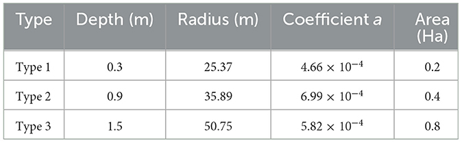
Table 2. Dimensions of three pothole types used in the hydrology module.
where the vertex is represented by (h, k), and a is a positive coefficient that depends on the shape of the profile. The pothole dimensions are chosen based on recent studies that have shown how the median pothole size to be 0.16 Ha, with areas ranging up to several hectares in sizes (Huang et al., 2011; Wu and Lane, 2016; Mcdeid, 2017) and observed pothole depths of 0.3–1.49 m for North Central Iowa (Upadhaya and Arbuckle, 2021).
To calculate flooding and crop death, the depth of ponding for each pothole is continuously computed at the hourly time step using the previous 24 h precipitation total (precip24hr, mm). Depth of ponding (mm) is based on the equation (Edmonds et al., 2021):
If an area within the pothole is flooded to a minimum depth of a 12.7 mm for a 24-h period or longer, complete crop death occurs. The final crop yield within the pothole area is represented by:
where Aflooded is the flooded area of the pothole and yieldsoil is the normal crop yield for each soil type in the pothole when no flooding occurs.
2.3.2. Crop yield module
Crop yields are modeled using a regression developed for Iowa by Tannura et al. (2008), which takes into account monthly precipitation and temperature:
Based on the mean error of the regression for Iowa over the 1960–2016 period, a correction factor of +0.395 MT/ha was added. Because each farmer agent's land is comprised of different soil types with different productivity, adjustments and stochastic variability are applied to the calculated yield (yieldsoil) for a specific soil type (Dziubanski et al., 2020).
2.4. Model timeline
The model proceeds as follows: in January, the farmer agent calculates his/her preferred land division between production and conservation (Figure 2). In February, the city agent contacts farmer agents in random order to establish new conservation contracts if an unmet conservation goal remains or to renew any expiring contracts. A new 10-year contract is established if the farmer agent wants to add additional conservation acreage. At this time, expiring contracts can be renewed at the same number of hectares or less, or ended. Any newly acquired conservation acreage is subtracted from the city agent's conservation goal established in January. The city agent continues to contact farmer agents until its conservation goal is met. If the conservation goal is not reached in a given year, the goal rolls into the next year. Prior to May, the farmer agent establishes any newly contracted conservation land on the historically poorest yielding land first. No further decision making occurs during May through August; however, during this time, a maximum discharge event occurs. In September, the associated flood damage cost is calculated by the city agent and used to determine how much land to allocate into conservation. If no flooding occurred, the conservation goal remains unchanged. In October, the farmer agent harvests his/her crop, and calculates yields and profits for that year.
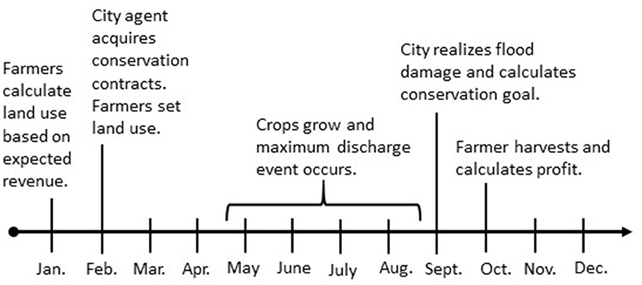
Figure 2. Annual timeline of agent decisions and actions in the model.
3. Model setup
The watershed in the model is based on the Ioway Creek watershed located in Central Iowa, USA (Figure 3). The Ioway Creek watershed is located within the Des Moines lobe, which is characterized by relatively flat and hummocky topography and poorly drained soils [Prior, 1991; USDA-Natural Resources Conservation Service (USDA-NRCS), 2015]. Prairie pothole depressions are a major feature in the region; they are prone to flooding, particularly during heavier rainfall in the months of May and June (Miller et al., 2009). Approximately 70% of the watershed is in row crop agriculture, with one major urban center (Ames, IA) at the outlet of the watershed. In the hydrology module, the watershed is represented through 14 subbasins and hydrologic parameters are taken from Dziubanski et al. (2020).
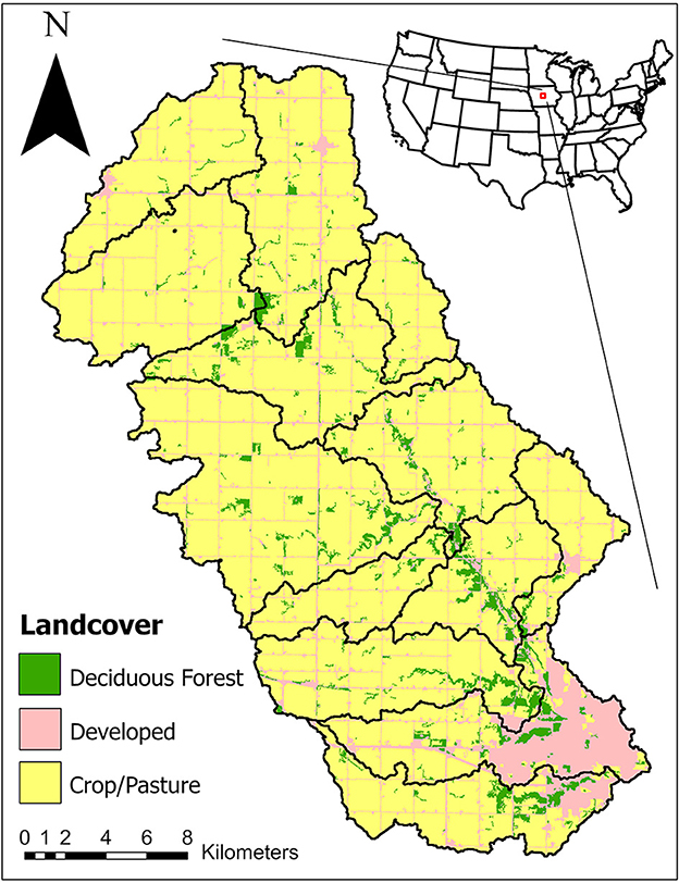
Figure 3. Ioway Creek watershed, land cover, and subbasin used in the hydrology module.
3.1. Model initialization
A total of 100 farmer agents are implemented in the model with approximately seven farmer agents allocated to each subbasin. Each farmer agent manages ~121.4 hectares of agricultural land with up to 8 different randomly assigned soil types. The percentage of each soil type is chosen from a uniform distribution, with the constraint that each soil type must encompass at least 0.1 Ha. In addition, each farmer agent's land is randomly characterized by up to 10% pothole land of Type1, Type2, and Type3, with the total acres of pothole land chosen from the uniform distribution . The upper value 12.14 Ha is based on each farmer agent having a total of 121.4 Ha of land.
Dziubanski et al. (2020) calibrated the ABM to this study region to reproduce the historical range and variability of land enrolled in the federal Conservation Reserve Program (CRP) for central Iowa (CRP is similar to the program offered by the city agent). The parameters found in that study are used here to assign values to farmer agents. Each farmer agent's Consmax parameter is randomly chosen from the Gaussian distribution , based on the optimal mean value of 0.06 for Consmax. Because the standard deviation of Consmax is unknown, a random value is chosen from the uniform distribution to represent the standard deviation. If the chosen Consmax is above or below the range 0.0–0.1 (Section 2.2.1), then Consmax is automatically set to either 0.1 or 0.0. Decision weights (Wrisk−averse, Wfutures, Wprofit, Wcons, Wneighbor) are initialized for each farmer agent from the Gaussian distribution , where the mean x is chosen from the uniform distribution The possible upper and lower bounds (x1, x2) of each decision variable are based on the previously calibrated values specified in Table 1. For example, the mean of Wrisk−averse could be anywhere in the range 0.1–0.43. Once the mean value x is chosen, the above Gaussian distribution is used to initialize the decision variables for all 100 farmer agents.
The city agent is located at the outlet of the watershed (i.e., the most downstream subbasin). The ConsGoallower and ConsGoalupper parameters of the city agent are set to 0.01 and 0.05, respectively (Table 1).
3.2. Model input
Historical crop prices ($/MT), crop production costs ($/Ha), cash rental rates ($/Ha), and federal government subsidy estimates ($/Ha) from the years 1970–2016 are used to drive the agent-based model. Federal crop subsidies are based on 16 years of historical estimates (2000–2016) (Hofstrand, 2018). Due to relative long-term stability in crop prices, it is assumed that federal crop subsidies from 1970 to 2000 are at a similar level to 2000–2005 and existed during the entire simulation period. All economic data was obtained from Iowa State University Agricultural Extension and Illinois FarmDoc.
Hourly precipitation and average daily temperature from the climate projections of the North American Coordinated Regional Climate Downscaling Experiment (NA-CORDEX) are used for future simulations, and historical 1970–2016 data is used for historical simulations. Data was obtained through the National Center for Atmospheric Research climate data gateway and the Earth System Grid Foundation. Five climate simulations are used, with varying combinations of global and regional models, as well as grid spacing and emission scenarios (Table 3) to represent a range of possible future temperature and precipitation. Of the five simulations, MPI.22.rcp85 and MPI.44.rcp85 have the warmest and wettest conditions by 2100. Each climate simulation was bias corrected using kernel density distribution mapping (KDDM) (Mcginnis et al., 2015). The KDDM technique calculates the probability distribution function (PDF) for each dataset, then uses trapezoidal integration to convert the PDFs to the corresponding cumulative distribution functions (CDF). With this technique, the historical climate simulations are bias corrected using historical data. That correction is then applied to the future climate simulations. The bias correction was conducted using hourly stage IV precipitation data (2002–2016) and daily mean temperatures (2000–2015) computed from hourly temperature data from the Ames, Iowa Automated Surface Observing System (ASOS).

Table 3. Climate simulations used in this study.
3.3. Scenario analysis
Simulations are conducted for the first half and second half of the 21st century using each climate scenario, with four different model configurations, and the 1970–2016 historical economic data (Table 4). The limited economic data time period required that the future simulations be divided into two 47-year periods (2018–2065 and 2050–2097). Applying the same economic conditions to each of the different climate scenarios and time periods allows for analysis of the climate effects on the outcomes of interest.
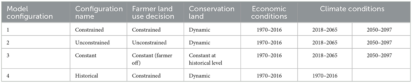
Table 4. Model configurations used in scenario analysis.
In model configuration 1, farmer decision-making is turned on, but the conservation land for each farmer agent is constrained by their ConsMax parameter (Table 4, row 1). This causes the preferences of the farmer agents to remain fixed through time as they cannot implement more conservation land than their ConsMax parameter allows, even if it would be economically beneficial. In model configuration 2, the ConsMax parameter of each farmer agent is allowed to change through time if the conservation decision becomes greater than his/her current ConsMax parameter (Table 4, row 2). This allows the farmer agents to become more conservation-minded over time in response to conditions.
In model configuration 3, farmer decision-making is turned off and conservation land is kept at the mean observed conservation land for the 2006–2016 period (Table 4, row 3). This simulation, in which future conditions are influenced only by the changing climate, is used to evaluate the impact of climate on streamflow and agent behavior in simulations when compared to model configuration 2. The unconstrained, dynamic simulations represent a combination of climate and human influence. Subtracting the two simulations (human impact = constant − unconstrained) isolates the impact of the agents on the hydrologic outcomes. Using this information, the percent contribution from the human impact and the climate impact is computed.
Finally, model configuration 4 uses historical climate data (1970–2016) with the farmer decision making turned on, but conservation land constrained by the ConsMax parameter (Table 4, row 4). The future simulations were analyzed against this historical simulation for changes in the annual 95th percentile discharge, conservation land, and the 10-year flood.
4. Results
4.1. Land use under future climate analysis
Under the constrained scenario (model configuration 1, Table 4) where farmer agents are allowed to modify their land use but are constrained by their ConsMax parameter, the mean 95th percentile discharge decreases on average by 6.5% relative to the constant scenario (model configuration 3) where conservation land is kept at the 2006–2016 mean (Figure 4, red). This 6.5% decrease from the constant scenario corresponds to the ~40–50% increase in conservation land from the historical mean (Figure 5, red). The historical mean 2006–2016 conservation land in the watershed was 3.7%, while the farmer agents implement 5.8% under future climate. Under almost all climate simulations, particularly during 2050–2097, farmer agents are implementing, on average, the maximum conservation land that his/her ConsMax parameter allows in the constrained scenario.
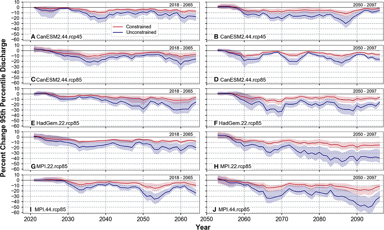
Figure 4. Means (solid lines) and ranges (shaded areas) of percent change in 95th percentile discharge for the constrained (red) and unconstrained (blue) scenarios relative to the constant scenario for 2018–2065 (A, C, E, G, I) and 2050–2097 (B, D, F, H, J).
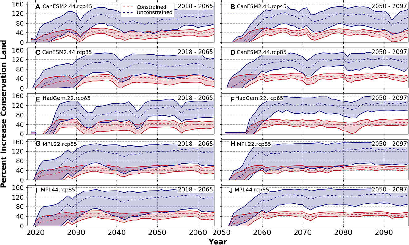
Figure 5. Means (dashed lines) and ranges (shaded areas) of percent change in conservation land for the constrained (red) and unconstrained (blue) scenarios relative to the constant scenario for 2018–2065 (A, C, E, G, I) and 2050–2097 (B, D, F, H, J).
For the constrained scenario, there is a slightly larger decrease in the mean 95th percentile discharge by the end of the 2050–2097 simulation period compared to the 2018–2065 period, particularly for the MPI simulations (Figures 4H, J, red). While the amount of conservation land generally increases and becomes more stable throughout both simulation periods, conservation land is more variable in the 2018–2065 period (Figure 5, red). Individual simulations show larger magnitudes of change for the 2018–2065 period, generally following changes in crop prices.
The unconstrained scenario (model configuration 2) where farmer agents are allowed to modify their land unconstrained by their ConsMax parameter, results in the mean 95th percentile discharge decreasing by 16% more on average compared to the constant scenario (Figure 4, blue). Under unconstrained conditions, conservation land increases by 80–120% relative to the constant land use scenario (Figure 5, blue). In addition, farmer agents transition from an initial mean ConsMax parameter of 0.06 to a mean ConsMax parameter of 0.067–0.09, depending on the model iteration. Thus, the farmer agents never implement on average more than 9% land conservation in any iteration of the model, which is below the theoretical maximum defined by Dziubanski et al. (2020). This percentage is also significantly lower than the highest conservation goal set by the city agent. Under the wetter conditions of 2050–2097, the city agent has a goal of converting over 80% of the watershed to conservation during certain simulations. While this amount of land conversion is unrealistic, it reflects the magnitude of the flood mitigation challenges facing the city.
The range in percent conservation land produced by the various model iterations is larger under the unconstrained conditions (Figure 5), and smallest under the wettest climates (i.e., RCP8.5 and the 2050–2097 period). For example, for constrained HadGem.22.rcp85 simulations (Figures 5E, F, red), farmer agents decrease conservation land during the 2030–2035 period from 50% to 10%, but the same decrease is not present around 2062–2067 even though the economics (i.e., crop prices, production costs, etc.) are identical for those years. This smaller amount of land use change may be due to the wetter climate in the second half of the century leading to more in-field flooding and lower crop yields. If yields drop due to climate conditions, economic changes, such as increased crop prices, may be insufficient to motivate the farmer agent to take land out of conservation, particularly when less profitable land is taken out of production first. As a result of the greater amount of conservation land, the increase in the mean 95th percentile discharge is mitigated to a slightly greater degree. A clear example occurs for the HadGEM simulations, where the change in the 95th percentile discharge for 2062–2067 is up to 30% lower compared to only 0–15% lower for 2030–2035 (Figures 4E, F).
4.2. Climate and human impact analysis
The watershed transitions to a higher flow regime (Figure 6) due to a wetter climate (Figure 7) starting around 2050, particularly under the RCP8.5 trajectory. Considering the constant land use scenario (model configuration 3), the mean 95th percentile discharge increases by 18% and 30% under the RCP4.5 and RCP8.5 trajectories, respectively, for the 2018–2065 period compared to mean 1970–2016 95th percentile discharge (Figure 6). The increase is larger during the 2050–2097 period, with average increases of 30% and 75% under the RCP4.5 and RCP8.5 trajectories, respectively.
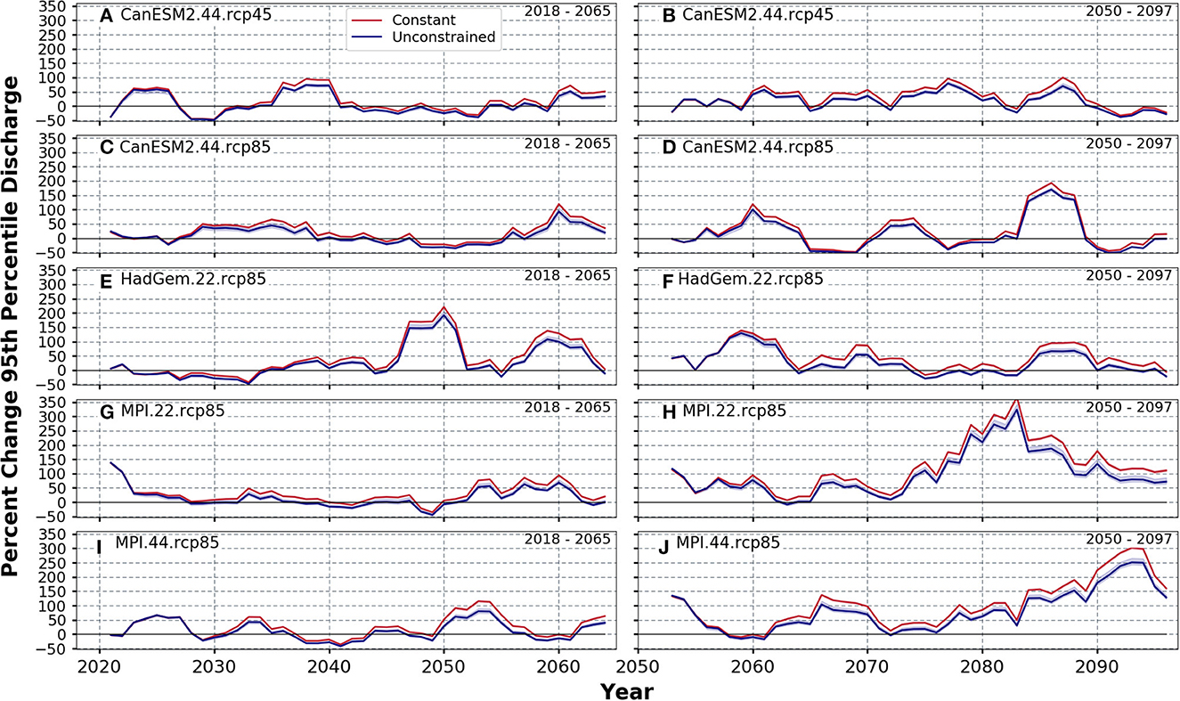
Figure 6. Percent change in 95th percentile discharge for the constant (red) and unconstrained (blue) scenarios compared to the mean 1970–2016 95th percentile discharge. (A, C, E, G, I) depict change for 2018–2065 and (B, D, F, H, J) depict change for 2050–2097.
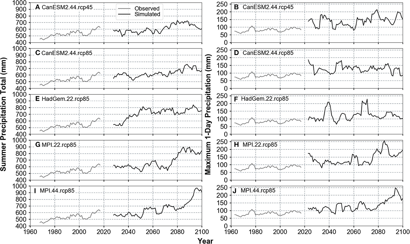
Figure 7. Trends in total precipitation (A, C, E, G, I) and maximum 1-day precipitation (B, D, F, H, J) for the summer months of April-August for the observed time series (gray) and climate simulations (black).
The CanESM2.44.rcp45 simulation shows the smallest changes in 95th percentile discharge, with most changes ranging between ±50% for both periods (Figures 6A, B). The CanESM2.44.rcp85 suggests significantly more variable flow in the future (2050–2097), with the 95th percentile flow 25–50% lower than the historical mean during certain periods and up to 200% higher during other periods, particularly during the latter half of the century (Figure 6D). Under the MPI.22.rcp85 and MPI.44.rcp85, changes in the mean 95th percentile flow are small in the first half of the century, and larger during the second half of the century (mean 95th percentile flow increases by 80–93% for the 2050–2097 period relative to the 2018–2065 period for the constant land use scenario) (Figures 6G–J). This increase in flow corresponds to the trends in precipitation present in the MPI simulations (Figures 7G–J). Total summer precipitation (April-August) increases by 160% under both MPI simulations by 2100 relative to historical observations.
In the latter half of the century, the difference between climate models increases. The MPI model is significantly wetter than the HadGEM model. Under the HadGEM simulation, flow is increased from 2045 to 2065, but from 2065 to 2085, peak flow is not significantly changed from the mean historical 95th percentile flow (Figures 4E, F). While the HadGEM model suggests that total summer precipitation will increase by 130% beyond 2040, this does not translate to consistent increased 95th percentile flow (Figure 7E). The MPI simulations, particularly the MPI.22.rcp85, show a transition to more intense 1-day precipitation beyond 2070, which combined with the increase in total summer precipitation, results in the >200% increase in mean 95th percentile flow (Figures 6H, J, 7H, J).
The effect of land use conversion (i.e., human impact) on decreasing peak streamflow can be seen in the difference between the constant and unconstrained scenarios. Under the RCP8.5 trajectory, the unconstrained scenario shows an average 16% increase in mean 95th percentile flow vs. a 29% increase under the constant scenario for the 2018–2065 period (Figures 6C, E, G, I). A similar result is observed for the 2050–2097 period, with a 55% increase in mean 95th percentile flow under the unconstrained scenario compared to the larger 75% increase under the constant scenario (Figures 6D, F, H, J).
The impact of human activities relative to climate on mean peak discharge is examined using the constant scenario to indicate climate impact, and the difference between the unconstrained and constant scenarios to indicate the human impact (Figure 8). During the 2018–2065 period, the human system more often has the greater influence on the 95th percentile discharge. The human system under the CanESM2 and MPI simulations, has up to an 80% impact on flow during certain periods, particularly when 95th percentile discharge is not significantly different from the historical (such as, 2040–2060) (Figures 6, 8A, C, G, I). The HadGEM model is the only simulation that deviates from the other models in the study, with a dominant climate impact from 2045 to 2065 (Figures 8E, F).
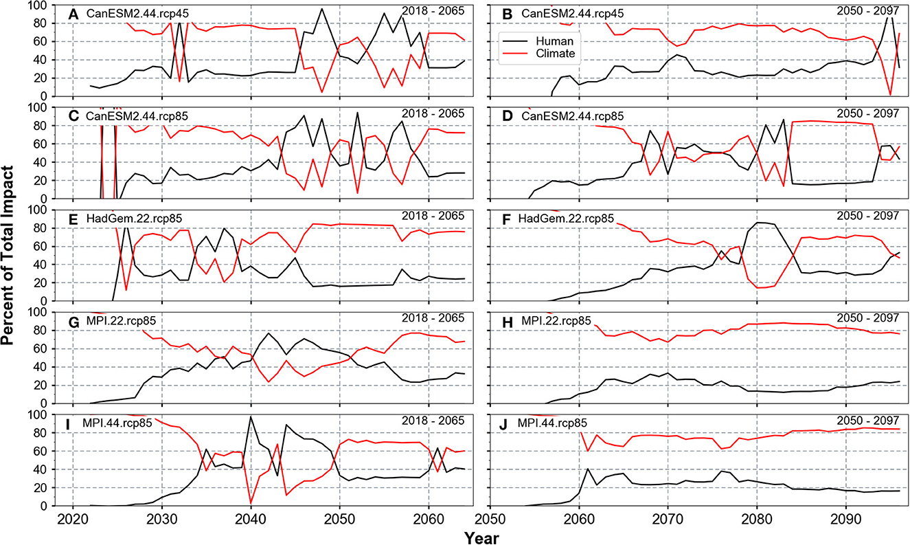
Figure 8. Percent of total impact on the 95th percentile discharge from the human system (black) and the climate system (red). (A, C, E, G, I) depict 2018–2065 and (B, D, F, H, J) depict 2050–2097.
All simulations indicate climate as having the dominant influence on discharge variability during the 2050–2097 period, particularly the CanESM2.44.rcp45 simulation and both MPI simulations (Figure 8). Approximately 60–90% of the change in mean 95th percentile discharge can be attributed to climate under the MPI scenarios during the latter half of the century, while only ~20% impact comes from the human system (Figures 8H, J). Likewise, the climate impact under the CanESM2.44.rcp45 simulation is 60–80% (Figure 8B).
4.3. Flood frequency analysis
There were seven 10-year flood events (defined using 1965–2018 observed discharge for the Ioway Creek watershed) present in the historical simulation (model configuration 4), which equates to an observed frequency of 0.14. This corresponds well with the actual observed frequency of 0.12 (6 years) for the 1970–2016 period (Figure 9). The 10-year flood event becomes more frequent in all future climate and land use scenarios, increasing up to 0.5 for the 2018–2065 period (Figure 9A), and up to 0.67 for the 2050–2097 period (Figure 9B). The constant land use scenario produces the greatest increase in the 10-year flood frequency, while the unconstrained scenario results in the lowest increase due to the implementation of more conservation land.
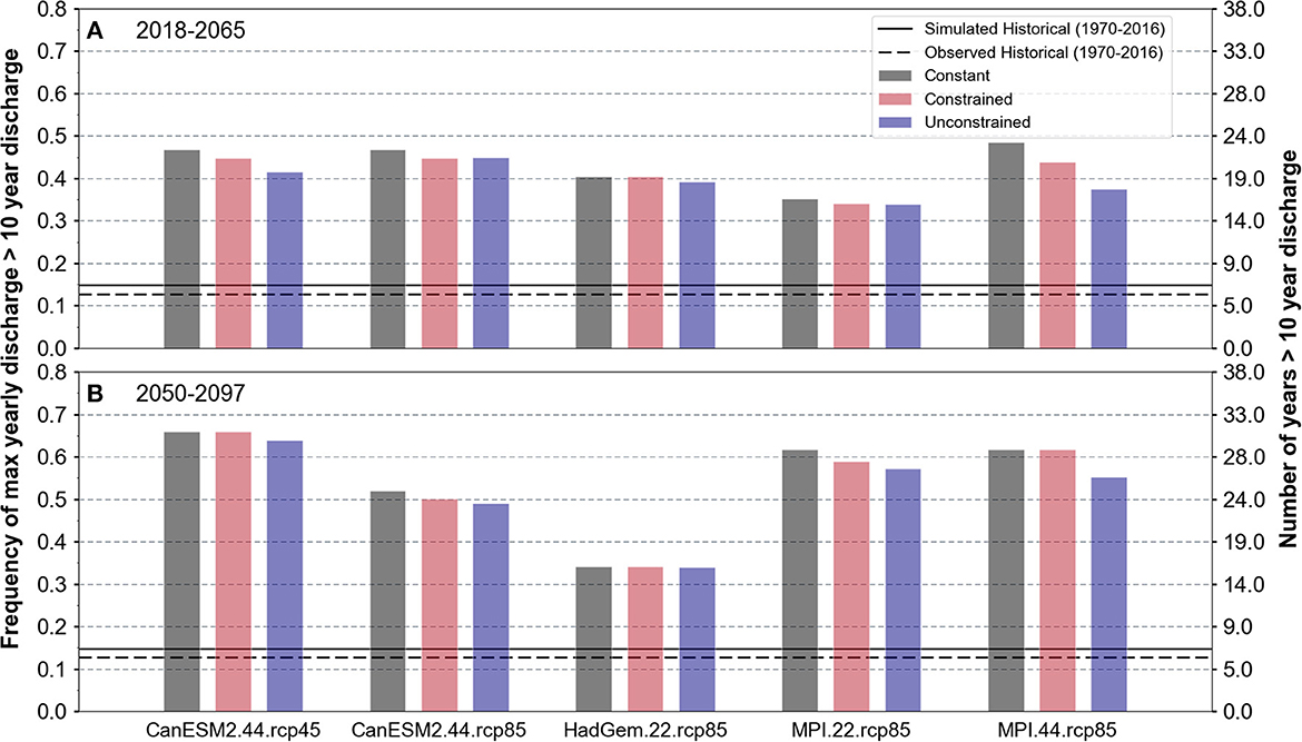
Figure 9. Frequency of maximum annual discharge exceeding the 10-year event discharge over the 47 year simulation period for 2018–2065 (A) and 2050–2097 (B).
The influence of land use on mitigating the increased frequency of the 10-year event is greater in the wettest scenarios (i.e., MIP.22.rcp85 and MPI.44.rcp85). The climate projections for which the human and climate impact were found to be more equal (Figures 8C–F), also the overall driest scenarios, result in the least differences between in the 10-year event frequency among the various land use configurations (Figure 9 CanESM2.44.rcp85 and HadGem.22.rcp85). In all cases, the impact of increased conservation land is not enough to substantially reduce the frequency of the 10-year flood under future climate. Under the MPI simulations, the human system reduces the number of years with flooding by 4–5. However, this reduction is small in comparison to the overall increase to more than 24 10-year flood during the 2050–2097 period.
5. Discussion
5.1. Land use under future climate
We used an agent-based model of a representative agricultural watershed to explore the response of a couple social-hydrologic system to increasing climate extremes and to understand the relative influence of climate and land use on hydrologic outcomes. We found that wetter future conditions lead farmer agents to adopt more conservation than under historical climate conditions. This land conversion lessens the degree to which the peak discharge increases. The range of simulated conservation land and 95th percentile discharge is much lower for scenarios in which more restrictions are placed on farmer decision making (constrained). In contrast, farmer agents indicate a willingness to go beyond their preset ConsMax when they are allowed to modify the maximum amount of land they can convert and these unconstrained scenarios result in greater uncertainty in modeled outcomes. However, the farmer population maxes out at a ConsMax of 8–9% by the end of 2050–2097, never reaching the maximum theoretical ConsMax value of 10% that we have defined for the model. This result would potentially be different with different economic factors, which in our case appear to be insufficient at motivating further adaptation. While the adoption of conservation land by the farmer agent decreased the mean 95th percentile discharge by a notable amount, the impact of the climate system on peak discharge outweighs that of the human system by the end of the century.
A number of our findings can arguably be extrapolated beyond the watershed studied to parts of the Midwest US where precipitation frequency and intensity are expected to increase (Janssen et al., 2014; Wuebbles et al., 2014), and rain-fed row crop farming is prevalent. Under analysis of CMIP5 model output conducted by Wuebbles et al. (2014), the Extreme Precipitation Index (Kunkel et al., 1999) for the North Central U.S region rises from about 0.4 and 0.6 for the 2016–2025 period to 0.6 and 1.9 for the end of the century under the RCP4.5 and RCP8.5 trajectories, respectively. Prein et al. (2017) drew similar conclusion about precipitation trends for the North Central U.S., with extreme precipitation increasing during the winter and summer months, and moderate precipitation decreasing during the summer. The precipitation used in this study shows that the intensity of 1-day maximum precipitation may increase by 50–100% during certain periods (e.g., MPI.44.rcp85, 2080–2100) with precipitation intensity increasing mostly during the months of May-July. Early summer increases in precipitation amount and intensity would contribute to early crop flooding and lower crop yields.
One of the primary drivers of land conversion in our simulations was lower yield due to the wetter climate. Yields produced by the model are 25% (2018–2065) and 30% (2050–2097) lower under the RCP4.5 scenarios compared to historical climate. This decrease in yield is even more substantial under the RCP8.5 scenarios, with a 27% and 42% decrease during the first and second half of the century, respectively. The trend of decreased yields in the future is supported by a number of studies (Schlenker and Roberts, 2009; Hatfield et al., 2011; Rosenzweig et al., 2014; Xu et al., 2016). Xu et al. (2016), who used the Agro-IBIS model driven by CMIP5 climate output, found yield to decrease by 13–42% under RCP4.5 and 17–50% under RCP8.5 for Iowa. Similarly, crop yields are shown to decrease by 30–46% by the end of the century in a study conducted by Schlenker and Roberts (2009). Farmers may need to find alternative sources of revenue under future climate if crop prices are not modified in response to yield declines in this region. In the case of this ABM, the farmers' only option is to implement more conservation land, guaranteeing a payment for the converted land. However, even in the unconstrained scenario, the mean ConsMax of the farmer population never exceeds 0.09 (or 9% of the watershed). This indicates that under climate change, row crop farming in the region of study could remain profitable relative to conservation incentives. Future studies should explore the impact of alternative conservation programs and increased monetary incentives.
5.2. Climate and human impacts on streamflow and flooding
As shown by our results and demonstrated by a number of studies (Cherkauer and Sinha, 2010; Frans et al., 2013; Naz et al., 2016; Teshager et al., 2016), increasing precipitation amount and intensity can be expected to lead to increases in discharge and more frequent floods across the Midwest U.S. Using CMIP5 data with the VIC model for HUC8 basins through 2050, Naz et al. (2016) found that runoff from most subbasins in the Midwest will increase by 6–30% during the March-May period. Additionally, their study shows that 95th percentile discharge increases by at least 5% for all subbasins in the region, with many subbasins showing an increase of 15–20% or more. A study by Cherkauer and Sinha (2010), which also used the VIC model to simulate watersheds in Illinois and Wisconsin, reports that seasonal average peak flows increase by ~10–20% for spring and summer under three climate scenario, with some watersheds showing a 20–30% increase. Similar to Cherkauer and Sinha (2010), in this study, the 95th percentile discharge increased by 29% for the 2018–2050 period when constant land use was used. By comparison, under the unconstrained scenario, when farmer decision making is turned on and land use varies in response to intrinsic and extrinsic factors, the increase in the 95th percentile discharge is only 16%. This results in a significantly smaller increase in large discharge events and illustrates the importance of considering the human system in hydrologic analyses (Montanari et al., 2013; Srinivasan et al., 2017). Models that incorporate a human system component provide an opportunity to explore multiple possible situations and solutions for better planning.
Although some streamflow mitigation may be realized through changes in the human system (i.e., land management), our finding is that climate could account for 60–80% of the changes seen in discharge by the latter half of the 21st century. While not every study has found that discharge will increase for the Midwest Corn belt region (Milly et al., 2002; Chien et al., 2013), several studies of observed data suggest that the potential for flooding across the Midwest is increasing and that much of that change is a result of changing precipitation patterns rather than land use changes (Tomer and Schilling, 2009; Steffens and Franz, 2012; Frans et al., 2013; Ryberg et al., 2014; Gupta et al., 2015; Mallakpour and Villarini, 2015). Tomer and Schilling (2009) for instance, found that climate has been the primary driver in changing discharge since the 1970s for four watersheds in Iowa and Illinois. The 1970s was a period of transition away from land use that included small grain and pastures to predominantly row crop cultivation, which is the land use modeled in our study. Other studies confirm that changes in precipitation have largely dominated changes in streamflow for watersheds in Iowa and Minnesota throughout the last century (Steffens and Franz, 2012; Frans et al., 2013; Gupta et al., 2015). Rogger et al. (2017) points out that many studies of land use and climate impacts on streamflow at the larger scale indicate climate to be the major driver in changing streamflow, whereas studies at the smaller field scale show a large impact from land use change. Thus, further work is needed to understand how land use change effects scale up to the size of a larger watershed or region, and in particular, how these scaling effects may be different in models that consider the human system as dynamic and changing. Further refinement of the social, economic, and natural systems of the model could be made to allow for consideration of alternative strategies. Future work exploring alternative economic and social scenarios would enhance and refine our results and support planning through exploration of alternative scenarios.
Data availability statement
The raw data supporting the conclusions of this article will be made available by the authors, without undue reservation.
Author contributions
All authors listed have made a substantial, direct, and intellectual contribution to the work and approved it for publication.
Funding
Funding for this project was provided by an Iowa State University, College of Liberal Arts and Sciences grant. The open access publication fees for this article were covered by the Iowa State University Library.
Acknowledgments
This study was previously published as a Ph.D. dissertation at Iowa State University in 2018 titled Investigating the impacts of human decision-making and climate change on hydrologic response in an agricultural watershed. We would like to thank all other grant participants, including Chris R. Rehmann, Jean Goodwin, William W. Simpkins, Leigh Tesfatsion, Dara Wald, and Alan Wanamaker.
Conflict of interest
The authors declare that the research was conducted in the absence of any commercial or financial relationships that could be construed as a potential conflict of interest.
Publisher's note
All claims expressed in this article are solely those of the authors and do not necessarily represent those of their affiliated organizations, or those of the publisher, the editors and the reviewers. Any product that may be evaluated in this article, or claim that may be made by its manufacturer, is not guaranteed or endorsed by the publisher.
References
Ahn, K. H., and Merwade, V. (2014). Quantifying the relative impact of climate and human activities on streamflow. J. Hydrol. 515, 257–266. doi: 10.1016/j.jhydrol.2014.04.062
Arbuckle, J. G., Prokopy, L. S., Haigh, T., Hobbs, J., Knoot, T., and Knutson, C. (2013). Climate change beliefs, concerns, and attitudes toward adaptation and mitigation among farmers in the Midwestern United States. Clim. Change 117, 943–950. doi: 10.1007/s10584-013-0707-6
Arnell, N. W., and Gosling, S. N. (2016). The impacts of climate change on river flood risk at the global scale. Clim. Change 134, 387–401. doi: 10.1007/s10584-014-1084-5
Carpenter, S. R., Cole, J., Pace, M. L., Batt, R., Brock, W. A., and Cline, T. (2011). Early warnings of regime shifts. Science (80-) 332, 1076–1079. doi: 10.1126/science.1203672
Chelsea Nagy, R., Graeme Lockaby, B., Kalin, L., and Anderson, C. (2012). Effects of urbanization on stream hydrology and water quality: the Florida Gulf Coast. Hydrol. Process. 26, 2019–2030. doi: 10.1002/hyp.8336
Cherkauer, K. A., and Sinha, T. (2010). Hydrologic impacts of projected future climate change in the Lake Michigan region. J. Great Lakes Res. 36, 33–50. doi: 10.1016/j.jglr.2009.11.012
Chien, H., Yeh, P. J. F., and Knouft, J. H. (2013). Modeling the potential impacts of climate change on streamflow in agricultural watersheds of the Midwestern United States. J. Hydrol. 491, 73–88. doi: 10.1016/j.jhydrol.2013.03.026
Christensen, N. S., Wood, A. W., Voisin, N., Lettenmaier, D. P., and Palmer, R. N. (2004). The effects of climate change on the hydrology and water resources of the Colorado River basin. Clim. Change 62, 337–363. doi: 10.1023/B:CLIM.0000013684.13621.1f
Cruise, J. F., Laymon, C. A., and Al-Hamdan, O. Z. (2010). Impact of 20 years of land-cover change on the hydrology of streams in the southeastern United States. J. Am. Water Resour. Assoc. 46, 1159–1170. doi: 10.1111/j.1752-1688.2010.00483.x
Davis, C. G., and Gillespie, J. M. (2007). Factors affecting the selection of business arrangements by U.S. hog farmers. Rev. Agric. Econ. 29, 331–348. doi: 10.1111/j.1467-9353.2007.00346.x
Dziubanski, D. J. (2018). Investigating the impacts of human decision-making and climate change on hydrologic response in an agricultural watershed. Grad. Theses Diss. 181p.
Dziubanski, D. J., Franz, K. J., and Gutowski, W. J. (2020). Linking economic and social factors to peak flows in an agricultural watershed using socio-hydrologic modeling. Hydrol. Earth Syst. Sci. 24, 2873–2894. doi: 10.5194/hess-24-2873-2020
Dziubanski, D. J., Franz, K. J., and Helmers, M. J. (2017). Effects of spatial distribution of prairie vegetation in an agricultural landscape on curve number values. J. Am. Water Resour. Assoc. 53, 365–381. doi: 10.1111/1752-1688.12510
Edmonds, P., Franz, K. J., Heaton, E. A., Kaleita, A. L., Soupir, M. L., and VanLoocke, A. (2021). Planting miscanthus instead of row crops may increase the productivity and economic performance of farmed potholes. GCB Bioenergy 13, 1481–1497. doi: 10.1111/gcbb.12870
Frans, C., Istanbulluoglu, E., Mishra, V., Munoz-Arriola, F., and Lettenmaier, D. P. (2013). Are climatic or land cover changes the dominant cause of runoff trends in the Upper Mississippi River Basin? Geophys. Res. Lett. 40, 1104–1110. doi: 10.1002/grl.50262
Granovetter, M. (1973). The strength of weak ties. Am. J. Sociol. 78, 1360–1380. doi: 10.1086/225469
Groisman, P. Y., Knight, R. W., and Karl, T. R. (2012). Changes in intense precipitation over the central United States. J. Hydrometeorol. 13, 47–66. doi: 10.1175/JHM-D-11-039.1
Gupta, S. C., Kessler, A. C., Brown, M. K., and Zvomuya, F. (2015). Climate and agricultural land use change impacts on streamflow in the upper midwestern United States. Water Resour. Res. 51, 5301–5317. doi: 10.1002/2015WR017323
Gutowski, W. J., Takle, E. S., Kozak, K. A., Patton, J. C., Arritt, R. W., and Christensen, J. H. (2007). A possible constraint on regional precipitation intensity changes under global warming. J. Hydrometeorol. 8, 1382–1396. doi: 10.1175/2007JHM817.1
Hatfield, J. L., Boote, K. J., Kimball, B. A., Ziska, L. H., Izaurralde, R. C., Ort, D. A., et al. (2011). Climate impacts on agriculture: implications for crop production. Agron. J. 103, 351–370. doi: 10.2134/agronj2010.0303
Helmers, M. J., Zhou, X., Asbjornsen, H., Kolka, R., Tomer, M. D., and Cruse, R. M. (2012). Sediment removal by prairie filter strips in row-cropped ephemeral watersheds. J. Environ. Qual. 41, 1531. doi: 10.2134/jeq2011.0473
Hernandez-Santana, V., Zhou, X., Helmers, M. J., Asbjornsen, H., Kolka, R., and Tomer, M. (2013). Native prairie filter strips reduce runoff from hillslopes under annual row-crop systems in Iowa, USA. J. Hydrol. 477, 94–103. doi: 10.1016/j.jhydrol.2012.11.013
Hofstrand, D. (2018). Tracking the Profitability of Corn Production. Ames, IA: Iowa State University Extension and Outreach.
Huang, S., Young, C., Feng, M., Heidemann, K., Cushing, M., Mushet, D. M., et al. (2011). Demonstration of a conceptual model for using LiDAR to improve the estimation of floodwater mitigation potential of Prairie Pothole Region wetlands. J. Hydrol. 405, 417–426. doi: 10.1016/j.jhydrol.2011.05.040
Janssen, E., Wuebbles, D., Kunkel, K., Olsen, S.C., and Goodman, A. (2014). Observational and model based trends and projections of extreme precipitation over the contiguous United States. Earth's Future, 2, 99–113. doi: 10.1002/2013EF000185
Karl, T. R., Melillo, J. M., and Peterson, T. C. (2009). Global Climate Change Impacts in the United States. New York, NY: Cambridge University Press, 196.
Karmalkar, A. V., and Bradley, R. S. (2017). Consequences of global warming of 1.5°c and 2°c for regional temperature and precipitation changes in the contiguous United States. PLoS ONE 12, 1–17. doi: 10.1371/journal.pone.0168697
Kunkel, K. E., Andsager, K., and Easterling, D. D. R. (1999). Long-term trends in extreme precipitation events over the conterminous United States and Canada. J. Clim. 12, 2515–2527. doi: 10.1175/1520-0442(1999)012<2515:LTTIEP>2.0.CO;2
Kwak, Y., and Deal, B. (2021). Resilient planning optimization through spatially explicit, Bi-directional sociohydrological modeling. Environ. Manag. J. 300, 113742. doi: 10.1016/j.jenvman.2021.113742
Mallakpour, I., and Villarini, G. (2015). The changing nature of flooding across the central United States. Nat. Clim. Chang. 5, 250–254. doi: 10.1038/nclimate2516
Mcdeid, S. M. (2017). Morphologic Characterization of Upland Depressional Wetlands on the Des Moines Lobe of Iowa. Ames, IA: Graduate Theses and Dissertations. 39p.
Mcginnis, S., Nychka, D., and Mearns, L. O. (2015). A New Distribution Mapping Technique for Climate Model Bias Correction. Machine Learning and Data Mining Approaches to Climate Science. Switzerland: Springer International Publishing, 91–99.
McGuire, J., Morton, L. W., and Cast, A. D. (2013). Reconstructing the good farmer identity: Shifts in farmer identities and farm management practices to improve water quality. Agric. Hum. Values 30, 57–69. doi: 10.1007/s10460-012-9381-y
Mearns, L. O., McGinnis, S., Korytina, D., Arritt, R., Biner, S., Bukovsky, M, et al. (2017). The NA-CORDEX Dataset, version 1.0. Boulder, CO: NCAR Climate Data Gateway. doi: 10.5065/D6SJ1JCH
Miller, B. A., Crumpton, W. G., and van der Valk, A. G. (2009). Spatial distribution of historical wetland classes on the Des Moines Lobe, Iowa. Wetlands 29, 1146–1152. doi: 10.1672/08-158.1
Milly, A. P. C. D., Betancourt, J., Falkenmark, M., Hirsch, R. M., Zbigniew, W., Lettenmaier, D. P., et al. (2008). Stationarity is dead: stationarity whither water management? Science (80-) 319, 573–574. doi: 10.1126/science.1151915
Milly, P. C. D., Wetherald, R. T., Dunne, K. A., and Delworth, T. L. (2002). Increasing risk of great floods in a changing climate. Nature 415, 514–517. doi: 10.1038/415514a
Montanari, A., Young, G., Savenije, H. H. G., Hughes, D., Wagener, T., and Ren, L. L. (2013). “Panta Rhei—Everything Flows”: Change in hydrology and society—The IAHS Scientific Decade 2013–2022. Hydrol. Sci. J. 58, 1256–1275. doi: 10.1080/02626667.2013.809088
Naik, P. K., and Jay, D. A. (2011). Distinguishing human and climate influences on the Columbia River: changes in mean flow and sediment transport. J. Hydrol. 404, 259–277. doi: 10.1016/j.jhydrol.2011.04.035
Naz, B. S., Kao, S. C., Ashfaq, M., Rastogi, D., Mei, R., and Bowling, L. C. (2016). Regional hydrologic response to climate change in the conterminous United States using high-resolution hydroclimate simulations. Glob. Planet. Change 143, 100–117. doi: 10.1016/j.gloplacha.2016.06.003
Newman, M. E. J., Watts, J., and Strogatz, S. H. (2002). Random graph models of social networks. Pnas 99, 2566–2572. doi: 10.1073/pnas.012582999
O'Keeffe, J., Moulds, S., Bergin, E., Brozovic, N., Mijic, A., and Buytaert, W. (2018). Including farmer irrigationbehavior in a sociohydrologicalmodeling framework with applicationin North India. Water Resour. Res. 54, 4849–4866. doi: 10.1029/2018WR023038
Prein, A. F., Rasmussen, R. M., Ikeda, K., Liu, C., Clark, M. P., and Holland, G. J. (2017). The future intensification of hourly precipitation extremes. Nat. Clim. Change 7, 48–52. doi: 10.1038/nclimate3168
Prokopy, L. S., Floress, K., Arbuckle, J. G., Church, S. P., Eanes, F. R., Gao, Y., et al. (2019). Adoption of agricultural conservation practices in the United States: evidence from 35 years of quantitative literature. J. Soil Water Conserv. 74, 520–534. doi: 10.2489/jswc.74.5.520
Rogger, M., Agnoletti, M., Alaoui, A., Bathurst, J. C., Bodner, G., and Borga, M. (2017). Land use change impacts on floods at the catchment scale: challenges and opportunities for future research. Water Resouces Res. 53, 5209–5219. doi: 10.1002/2017WR020723
Rosenzweig, C., Elliott, J., Deryng, D., Ruane, A. C., Müller, C., and Arneth, A. (2014). Assessing agricultural risks of climate change in the 21st century in a global gridded crop model intercomparison. Proc. Natl. Acad. Sci. U. S. A. 111, 3268–3273. doi: 10.1073/pnas.1222463110
Ross, A. R., and Chang, H. (2021). Modeling the system dynamics of irrigators' resilience to climate change in a glacier-influenced watershed. Hydrol. Sci. J. 66, 1743–1757. doi: 10.1080/02626667.2021.1962883
Ryberg, K., Lin, W., and Vecchia, A. (2014). Impact of climate variability on runoff in the North_central United States. J. Hydrol. Eng. 19, 148–158. doi: 10.1061/(ASCE)HE.1943-5584.0000775
Saltiel, J., Bauder, J. W., and Palakovich, S. (1994). Adoption of sustainable agricultural practices: diffusion, farm structure, and profitability. Rural Sociol. 59, 333–349. doi: 10.1111/j.1549-0831.1994.tb00536.x
Scharffenberg, W. A. (2013). Hydrologic Modeling System User's Manual. United State Army Corps Eng. Available online at: http://www.hec.usace.army.mil/software/hec-hms/documentation/HEC-HMS_Users_Manual_4.0.pdf (accessed 05, 2019).
Schilling, K. E., Chan, K. S., Liu, H., and Zhang, Y. K. (2010). Quantifying the effect of land use land cover change on increasing discharge in the Upper Mississippi River. J. Hydrol. 387, 343–345. doi: 10.1016/j.jhydrol.2010.04.019
Schlenker, W., and Roberts, M. J. (2009). Nonlinear temperature effects indicate severe damages to U.S. crop yields under climate change. Proc. Natl. Acad. Sci. U. S. A. 106, 15594–15598. doi: 10.1073/pnas.0906865106
Schmieg, S., Franz, K., Rehmann, C., and van Leeuwen, J. (2011). Reparameterization and Evaluation of the HEC-HMS Modeling Application for the City of Ames. Ames, IA: Iowa State University.
Sivapalan, M., Savenije, H. H. G., and Blöschl, G. (2012). Socio-hydrology: a new science of people and water. Hydrol. Process. 26, 1270–1276. doi: 10.1002/hyp.8426
Srinivasan, V., Sanderson, M., Garcia, M., Konar, M., Blöschl, G., and Sivapalan, M. (2017). Prediction in a socio-hydrological world. Hydrol. Sci. J. 62, 338–345. doi: 10.1080/02626667.2016.1253844
Steffens, K. J., and Franz, K. J. (2012). Late 20th-century trends in Iowa watersheds: an investigation of observed and modelled hydrologic storages and fluxes in heavily managed landscapes. Int. J. Climatol. 32, 1373–1391. doi: 10.1002/joc.2361
Tannura, M. A., Irwin, S. H., and Good, D. L. (2008). Weather, Technology, and Corn and Soybean Yields in the U.S. CornBelt, Marketing and Outlook Research Report 2008-01. Department of Agricultural and Consumer Economics, University of Illinois at Urbana-Champaign, Champaign, IL, United States. Available online at: http://www.farmdoc.uiuc.edu/marketing/morr/morr_archive.html
Teshager, A. D., Gassman, P. W., Schoof, J. T., and Secchi, S. (2016). Assessment of impacts of agricultural and climate change scenarios on watershed water quantity and quality, and crop production. Hydrol. Earth Syst. Sci. 20, 3325–3342. doi: 10.5194/hess-20-3325-2016
Tigner, R. (2006). Partial Budgeting: A Tool to Analyze Farm Business Changes. Ames, IA: Iowa State University Extension and Outreach.
Tomer, M. D., and Schilling, K. E. (2009). A simple approach to distinguish land-use and climate-change effects on watershed hydrology. J. Hydrol. 376, 24–33. doi: 10.1016/j.jhydrol.2009.07.029
Turner, R. E., and Rabalais, N. N. (2003). Linking landscape and water quality in the Mississippi river basin for 200 years. Bioscience 53, 563–572. doi: 10.1641/0006-3568(2003)053[0563:LLAWQI]2.0.CO;2
Upadhaya, S., and Arbuckle, J. G. (2021). Examining factors associated with farmers' climate-adaptive and maladaptive actions in the Midwest, U. S. Front. Clim. 3, 677548. doi: 10.3389/fclim.2021.677548
USDA-Natural Resources Conservation Service (USDA-NRCS) (2004). National Engineering Handbook, Part 630. Washington, DC.
USDA-Natural Resources Conservation Service (USDA-NRCS) (2015). Field Office Technical Guide. Availaable online at: http://www.nrcs.usda.gov/wps/portal/nrcs/main/national/technical/fotg/ (accessed April 9, 2016).
Van Vuuren, D. P., Edmonds, J., Kainuma, M., Riahi, K., Thomson, A., and Hibbard, K. (2011). The representative concentration pathways: an overview. Clim. Change 109, 5–31. doi: 10.1007/s10584-011-0148-z
Villarini, G., Smith, J. A., and Vecchi, G. A. (2013). Changing frequency of heavy rainfall over the central United States. J. Clim. 26, 351–357. doi: 10.1175/JCLI-D-12-00043.1
Wang, D., and Cai, X. (2010). Comparative study of climate and human impacts on seasonal baseflow in urban and agricultural watersheds. Geophys. Res. Lett. 37, 1–6. doi: 10.1029/2009GL041879
Wu, Q., and Lane, C. R. (2016). Delineation and quantification of wetland depressions in the Prairie Pothole Region of North Dakota. Wetlands 36, 215–227. doi: 10.1007/s13157-015-0731-6
Wuebbles, D., Meehl, G., Hayhoe, K., Karl, T. R., Kunkel, K., and Santer, B. (2014). CMIP5 climate model analyses: climate extremes in the United States. Bull. Am. Meteorol. Soc. 95, 571–583. doi: 10.1175/BAMS-D-12-00172.1
Xu, H., Twine, T. E., and Girvetz, E. (2016). Climate change and Maize Yield in Iowa. PLoS ONE 11, 1–20. doi: 10.1371/journal.pone.0156083
Ye, X., Zhang, Q., Liu, J., Li, X., and Xu, C. Y. (2013). Distinguishing the relative impacts of climate change and human activities on variation of streamflow in the poyang lake catchment, china. J. Hydrol. 494, 83–95. doi: 10.1016/j.jhydrol.2013.04.036
Zhang, X., Wan, H., Zwiers, F. W., Hegerl, G. C., and Min, S. K. (2013). Attributing intensification of precipitation extremes to human influence. Geophys. Res. Lett. 40, 5252–5257. doi: 10.1002/grl.51010
Keywords: agent-based modeling (ABM), climate change, land use, flooding, adaptation
Citation: Dziubanski D and Franz KJ (2023) Projecting hydrologic change under land use and climate scenarios in an agricultural watershed using agent-based modeling. Front. Water 5:1020080. doi: 10.3389/frwa.2023.1020080
Received: 19 August 2022; Accepted: 01 February 2023;
Published: 24 February 2023.
Edited by:
Yaoping Wang, The University of Tennessee, Knoxville, United StatesCopyright © 2023 Dziubanski and Franz. This is an open-access article distributed under the terms of the Creative Commons Attribution License (CC BY). The use, distribution or reproduction in other forums is permitted, provided the original author(s) and the copyright owner(s) are credited and that the original publication in this journal is cited, in accordance with accepted academic practice. No use, distribution or reproduction is permitted which does not comply with these terms.
*Correspondence: Kristie J. Franz,  a2ZyYW56QGlhc3RhdGUuZWR1
†These authors have contributed equally to this work