 Leila C. Hernandez Rodriguez
 Allison E. Goodwell
 Praveen Kumar
- 1Department of Civil and Environmental Engineering, University of Illinois at Urbana-Champaign, Champaign, IL, United States
- 2Department of Civil Engineering, University of Colorado Denver, Denver, CO, United States
- 3Department of Atmospheric Sciences, University of Illinois at Urbana-Champaign, Champaign, IL, United States
Eddy covariance measurements quantify the magnitude and temporal variability of land-atmosphere exchanges of water, heat, and carbon dioxide (CO2) among others. However, they also carry information regarding the influence of spatial heterogeneity within the flux footprint, the temporally dynamic source/sink area that contributes to the measured fluxes. A 25 m tall eddy covariance flux tower in Central Illinois, USA, a region where drastic seasonal land cover changes from intensive agriculture of maize and soybean occur, provides a unique setting to explore how the organized heterogeneity of row crop agriculture contributes to observations of land-atmosphere exchange. We characterize the effects of this heterogeneity on latent heat (LE), sensible heat (H), and CO2 fluxes (Fc) using a combined flux footprint and eco-hydrological modeling approach. We estimate the relative contribution of each crop type resulting from the structured spatial organization of the land cover to the observed fluxes from April 2016 to April 2019. We present the concept of a fetch rose, which represents the frequency of the location and length of the prevalent upwind distance contributing to the observations. The combined action of hydroclimatological drivers and land cover heterogeneity within the dynamic flux footprint explain interannual flux variations. We find that smaller flux footprints associated with unstable conditions are more likely to be dominated by a single crop type, but both crops typically influence any given flux measurement. Meanwhile, our ecohydrological modeling suggests that land cover heterogeneity leads to a greater than 10% difference in flux magnitudes for most time windows relative to an assumption of equally distributed crop types. This study shows how the observed flux magnitudes and variability depend on the organized land cover heterogeneity and is extensible to other intensively managed or otherwise heterogeneous landscapes.
1. Introduction
Agricultural landscapes dominate the US Midwest, influencing ecohydrological responses where the root-soil-canopy-atmosphere continuum act as an integrated system. In this region, small-grain production was replaced about a century ago by maize and soybean row crop agriculture. Today, a seasonal human-induced reorganization of vegetation to meet agricultural ecosystem services determines their spatial distribution (Richardson and Kumar, 2017), and the region experiences seasonal transitions in land cover every year. Specifically, row crop agriculture consists of seed planting in early spring, rapid growth in early summer, maturity in late summer, and harvest during autumn. During July, the US corn belt is now 40% more productive than the Amazonian rainforest (Foufoula-Georgiou et al., 2015) as a result of steady agricultural intensification over the past two centuries. In the Midwestern US, fertilization plays a critical role in agricultural intensification. Fertilization refers to the process of adding nutrients to the soil, such as nitrogen, phosphorus, and potassium, to improve crop growth and yields. This high level of fertilization is necessary to meet the demand for food and biofuel production, contributing to the region's agricultural productivity and competitiveness. This dense vegetated land cover during the growing season contrasts drastically with an almost bare landscape of soil, roots, and litter left after harvest typically around mid-October to November (NASS, 2010). During the growing season, a patchy mosaic of different crops is the dominant landscape feature, which partially hides other sources of heterogeneity such as soil properties and micro-topographic variability (Le and Kumar, 2014). In this study we examine the effects of the “organized land cover heterogeneity,” a term referring to the human-altered spatial organization of the vegetation in the landscape. Our focus is on the flux exchange between the landscape and the atmosphere, observed through measurements at an eddy covariance tower that encompasses the entire agricultural system, rather than just individual plots or fields. The organized heterogeneity results from human decisions regarding cropping patterns in the fields, crop rotation practices, and planting and harvesting times, which are distinct from naturally arising self-organized randomly distributed heterogeneity. For example, in an intensively managed landscape dominated by maize and soybean fields, such as that located in Illinois, a 25 m tall flux tower sees hundreds of agricultural plots in its contributing area that constantly shifts as a result of wind speed, direction, and atmospheric stability and influences its measurements of land-atmosphere exchanges of heat, water, and carbon dioxide (CO2) (Kirby et al., 2008). We quantitatively address one of the major challenges facing the interpretation of eddy covariance measurements in heterogeneous landscapes: Besides other sources of landscape heterogeneity, how can we partition the contributions of the human-induced “organized land cover heterogeneity” to the fluxes observed of a 25 m tall eddy covariance flux tower? Further, we evaluate the relative contribution of each crop type to the dynamics of the observed fluxes.
Eddy covariance measurements require a homogeneous flow field to provide an accurate integration of fluxes at the land-atmosphere interface (Aubinet et al., 2012; Burba, 2013). However, for a 25 m tall tower the dynamic upwind surface area where the land-atmosphere exchange flux is generated, known as the flux footprint, generally exhibits spatial heterogeneities and fluxes from different sources mix at the observation point (Leclerc and Foken, 2014). The use of footprint models for interpreting micrometeorological observations is a common practice, but the process of differential weighting within a temporally varying flux footprint is a “well-known but frequently overlooked feature of eddy covariance measurements” (Tuovinen et al., 2019; Chu et al., 2021). Previous studies have related eddy covariance flux tower observations to individual land use, mostly using a combination of different measurement techniques at different scales. One approach relies on in situ data, from nearby towers at which flux footprints cover a specific vegetation type (Biermann et al., 2014; Chi et al., 2019, 2020) or from flux chamber measurements (Tuovinen et al., 2019). However, in highly heterogeneous systems with mixed vegetation and soil wetness, it is known that there is a possibility for a serious mismatch between eddy covariance flux measurements and in situ measurements for determining specific fluxes associated with land cover classes (Alfieri et al., 2012; Wang et al., 2016; Tuovinen et al., 2019). In our case, when tens of plots are located inside the several square kilometer dynamic flux footprint, on-site measurements might not be representative of the average behavior of each land cover type inside the tower flux footprint, which can potentially bias the conclusions of a study. Typically, the use of in situ techniques, such as flux chambers, and remote sensing including aircraft data are limited to study cases. Previous studies have focused on extracting time series associated with a plot near a flux tower. In that case, the time series for the plot is obtained by extracting the observed fluxes when the plot intermittently lies within the dynamically changing flux footprint. For that purpose TOVI software (Licor, 2021), provides a set of analytical tools to examine eddy covariance flux and meteorological datasets. It is particularly advantageous for sites located in the upwind direction of the observing tower, as the area of interest can be consistently monitored. However, it often requires additional sources of information such as nearby towers or flux chambers, to later recreate a full time-series for a plot. Previous studies have also used a set of towers with overlapping flux footprints and modeling results for the times when the towers do not see the area of interest (Biermann et al., 2014). An alternative approach to estimating the contribution of individual crops to the total flux observed at the tower at each period is using a statistical approach to deconvolve the contributions from different types of vegetation (Tuovinen et al., 2019). However, we would require a large amount of data to not lose resolution at times when the flux tower only observes a small area of a certain field (e.g., if the wind does not blow from a specific direction), otherwise, it is not possible to get an estimation for a given field. To overcome these challenges, we combine multiple sources of information to synergistically inform the flux tower observations at the ecosystem scale and to decompose the relative contribution of each of the land cover types inside the flux footprint.
Our work is distinct from these previous efforts in that we combine observations and ecohydrological modeling to disentangle the contributions of different crop types to the observed fluxes where organized landscape heterogeneity dictates their relative contributions. In particular, it is distinct from and provides further refinement to the approach by Chu et al. (2021), which proposes monthly footprint climatologies for Ameriflux sites, in that we consider a structured heterogeneity inside the flux footprint whose contribution is dynamically changing at every measurement time step (15 min). When aggregating over time, the flux footprint climatology blends the sources and sinks of the flux while identifying the spatial extent and temporal dynamics of the areas contributing to the observed fluxes at a tower site. We adopt a more detailed perspective to analyze the relative contribution of each land cover type inside the dynamic flux footprint at each observational time step that results in clear identifications of the contribution to the observation from each crop type. The distinctive contribution of this study is to quantify the relative contribution of each land cover type inside the flux footprint on the measured exchange of water, heat, and CO2 fluxes at the land-atmosphere interface, which is a critical aspect when accounting for fluxes' sources and sinks from agricultural landscapes (Masson-Delmotte et al., 2021). Using the observations at the 25 m tall eddy covariance flux tower and other available data sources in a complementary way, such as flux footprint and ecohydrological modeling results, we can provide a more informed interpretation of the behavior of the observed fluxes with respect to their origin in the landscape. Our combined framework can be used to study aspects of landscape heterogeneity beyond what a tower could provide.
This paper is organized as follows: In Section 2, we describe the Intensively Managed Landscape Critical Zone Observatory (IMLCZO) study site (Wilson et al., 2018), and in Section 3, we present the methods to account for organized land cover spatial heterogeneity, including the considerations for the estimation of the two-dimensional flux footprint and the description of the use of the ecohydrological model to estimate the fluxes of the upwind area sources. Results and discussion are presented in Section 4, where we describe the ecosystem behavior at the study site as observed by the flux tower. Then we explain the results of the flux footprint and the ecohydrological modeling, and we analyze the seasonal and inter-annual evolution of the flux contribution due to each crop type. At the end of Section 4, we connect maize and soybean crop yield at the study site to investigate CO2 flux dynamics. In Section 5 we summarize the main findings and discuss some assumptions used in this work that could be relaxed in future studies.
2. Study site
2.1. Description
We use hydrometeorological data and flux measurements from a 25 m tall eddy covariance flux tower in the IMLCZO, located at 40.155N, 88.578W, Goose Creek Township, Piatt County, Illinois, US (Figure 1). In the Upper Sangamon River Basin, both glacial and management legacies have shaped soils, topography, and native land cover resulting in a low-relief landscape with poorly drained soils (Anders et al., 2018; Kumar et al., 2018). Therefore, the use of tile drains is a common practice in crop fields for subsurface drainage (Wilson et al., 2018). The climate at the study site is humid continental (Koppen climate classification Dfa) with warm and humid summers and cold winters. Historically, maximum precipitation occurs in late spring and early summer (i.e., April to June) with an average of about 100 mm per month and long-term observations have shown that Illinois has become wetter during the crop-growing season (Mishra and Cherkauer, 2010).
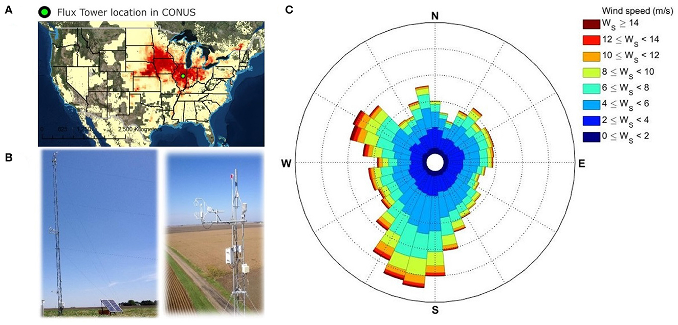
Figure 1. Goose Creek flux tower location and components. (A) Location of the tower (green dot) and the intensity of maize cultivation [the red area represents the corn harvested area fraction (high = red, low = light ivory); Monfreda et al., 2008]. (B) Fluxes measured by the 25 m tall eddy covariance tower come from the underlying heterogeneous landscape consisting of a mosaic of maize and soybean fields, from a fetch that can reach up to 10 km upwind from the tower. (C) The prevailing wind direction is from the southwest (4/23/2016–4/30/2019). The relative frequency with which the wind blows from a particular direction is proportional to the spoke's length, and colors indicate different wind speed categories.
In this agricultural landscape, vegetation dynamics are a strong determinant of land-atmosphere fluxes and their seasonality in the landscape. These dynamics are highly influenced by the prevalent practice of crop rotation between maize and soybean fields every one or two years, along with different intensities of tillage (Wilson et al., 2018). The region has a return of one harvest per year. Planting occurs from early April to late May, and harvest occurs from late September to early November. Maize is typically planted before soybean and harvested after, such that it has a longer growing season (NASS, 2010). In this study, we consider an April–March window as a “crop year” (e.g., April 2016 to March 2017 is denominated in this study as “crop year 2016”). Both crops have a peak vegetation cover with very dense leaf area index (LAI) reaching 4 for maize and 6–7 for soybean (Drewry et al., 2010). A distinctive feature of this agricultural region is how the dense vegetation cover during the growing season contrasts drastically with the almost bare landscape left after harvest until the following spring season when planting occurs (NASS, 2010) (Figure 2). Corn and soybean crops desiccate in the field prior to harvest, leading to the cessation of photosynthesis. After harvest, crop residues, i.e., mainly litter, stover, and plant roots, remain on the surface and in the shallow soil layers until the following spring when planting occurs (Warner et al., 1989).
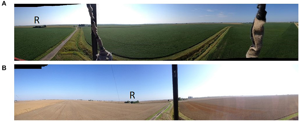
Figure 2. Panoramic view of the intensively managed agricultural study site. (A) During the growing season in July 2015, a row crop agriculture mosaic dominates the landscape, masking features such as micro-topographic depressions and soil variability. The vegetated land cover connects the heterogeneous ecosystem and the overlaying atmosphere during the growing season. (B) Right after harvest (October 2017) only litter remains over the surface. “R” marks a common reference point between the two pictures [Photo credit: (A) AG and (B) LH].
2.2. Instrumentation and data
Our 25 m-tall eddy covariance flux tower sees the combined response of hundreds of different plots every 15-min in the “patchwork quilt” landscape inside its several square kilometer dynamic flux footprint. We use a set of detailed land cover maps (NASS, 2018) to characterize the annually varying spatial land cover type distribution. Although the underlying vegetation is non-homogeneous, the tower is situated on terrain that is generally flat in all directions for an extended distance upwind, making the study site ideal to explore land-atmosphere flux dynamics resulting from land cover changes in a human-induced agricultural landscape. The eddy covariance tower has recorded data from April 2016 to the present day. The high-frequency instruments that estimate fluxes from the ecosystem are deployed at 25 m height (Li-7500 Infrared Gas Analyzer manufactured by LiCor Inc., and CSAT3 Sonic Anemometer manufactured by Campbell Scientific Ltd) (see Supplementary material). These instruments sample at 10 Hz and are set to record 15-minute averages. They point to the south-southwest, the prevailing wind direction (Figure 1). However, constantly shifting wind directions with meteorological conditions have implications for this study (described in detail in Section 3). For more information on the variables used in the analysis and instrumentation at this flux tower, see the Supplementary material.
3. Methods
Here we describe how we estimate the relative contribution of different land cover types to land-atmosphere fluxes measured at the flux tower. First, we use the wind data to obtain the variability of the areal coverage by using a two-dimensional flux footprint parameterization. Then we use a process-based ecohydrological model to obtain the temporally varying ratio of the flux values for different land covers. We use both the observed data and the modeled ratio of fluxes to estimate the contribution of each crop to the observed fluxes. From this, we can characterize the patterns of magnitude and variability of fluxes. Knowing that the observed fluxes at the ecosystem scale also carry the influence of the spatial heterogeneity within the flux footprint, we deconvolve the signal of the eddy covariance observation by quantifying the differential weighting of the plots based on the land cover types inside its dynamic flux footprint to find the relative contribution of each land cover type on the observations.
3.1. Estimation of two-dimensional flux footprint
Latent heat (LE), sensible heat, (H), and CO2 fluxes (Fc) estimated by the flux tower at any given time point correspond to an uncertain origin on the landscape. This origin can be estimated as the flux footprint, which is defined as the upwind landscape area that contributes to the measured vertical flux or concentration at a specific time (Vesala et al., 2008; Burba, 2013; Kljun et al., 2015). In this study, we use the two-dimensional flux footprint prediction model (FFP) proposed by Kljun et al. (2015), which considers the effects of surface roughness, atmospheric stability, and the crosswind spread of the footprint. For an agricultural landscape, surface roughness length changes as a function of vegetation height through the growing season. Also, atmospheric thermal stability rapidly changes with air temperature and density at a given pressure, impacting the vertical motion of air parcels. As a result, the areal contribution associated with each land cover type changes dynamically. The FFP model provides the width and shape of the two-dimensional flux footprint at any given time, where the source/sink area of the fluxes is located on the horizontal surface (x, y), and the tower height in the vertical direction, z (Figure 3). The FFP model assumes stationarity over the eddy-covariance integration period (here, 15-min) and horizontal homogeneity of the flow, but not of the scalar source/sink distribution. The variability of roughness over corn and soybean crops, however, can introduce potential errors in this assumption. These errors can include inaccuracies in the estimation of flow parameters, such as velocity and scalar transport.
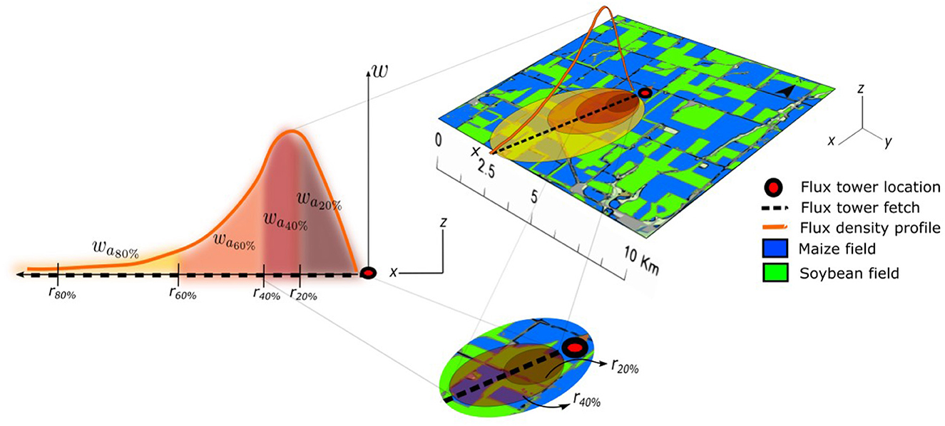
Figure 3. Illustration of a two-dimensional flux footprint that captures the organized heterogeneity of the maize-soybean mosaic. The land cover data from USDA 2016 (right) shows a mosaic of maize and soybean surrounding the flux tower. The density profile over the mosaic (orange) represents the relative contribution of the flux footprint as a function of the upwind distance, denominated as the fetch (black dashed line). Here we consider explicitly the dependence of the distance of the contributions from different patches. The density profile shows that higher contributions come from locations close to the tower, but not immediately underneath. In the two-dimensional approach (Kljun et al., 2015), the area defined by a set of contours (r%) of an increased percentage of contribution (bottom) define the strength and location of the sources/sink areas that contribute to the flux estimated at the tower. w is the weighted flux footprint contribution of each patch of area (a) defined by a given contour. Therefore, the flux tower measurement is the combined response of the fields inside the flux footprint (left).
When estimating the two-dimensional flux footprint, at each time interval the observed fluxes have their origin in a different combination of maize or soybean fields. To derive the source area up to a certain percent of flux contribution, we define a set of five contours (r) that define the areas that contribute 20, 40, 60, 80, and 90% of the total flux estimated by the flux tower. At farther locations beyond r90% that correspond to a contribution of 90%, the contributions tail off, so we limit our study to r90% (we use r% or r to represent percentage or equivalent fractional contribution, respectively). The associated fetch changes direction and length at every time step. In this context, the fetch is the distance from the tower to a specific fraction of the flux contribution. For example, the fetch for a 50% contribution (r50%) will be shorter than for a 90% contribution (r90%) (Burba, 2013).
We used the FFP model as a function on a loop in our Python code to estimate flux footprints for each 15-min data point from April 2016 to April 2019. Here we describe the inputs required for the FFP model. The calculation of the boundary layer height, blh, is based on the bulk Richardson number, Ri, method (Vogelezang and Holtslag, 1996) which is suitable for convective and stable boundary layer conditions and has been used in several previous studies (Seidel et al., 2012; Lee and De Wekker, 2016). We used the blh retrieved from the fifth generation reanalysis dataset for the global climate and weather, ERA5 (ECMWF, 2018) from the European Centre for Medium-Range Weather Forecasts (ECMWF). Near-surface atmospheric turbulence is caused by thermal and mechanical effects. Thermal turbulence is produced by temperature gradients and buoyant forces, while mechanical turbulence is generated by friction forces driven by wind shear, and therefore both control atmospheric fluxes. To account for atmospheric stability we calculate the Obukhov length, L (Foken, 2006), which is positive for stable and negative for unstable atmospheric stratification, and becomes near-infinite in the limit of neutral stratification. The standard deviation of the lateral velocity fluctuations, σv, is estimated using the 15-minute root-mean-square of the cross main-wind component, v, from the high-frequency data at the flux tower. In footprint modeling, changes in roughness are relevant when differences between land surface covers are significant (e.g., at the same time because of different vegetation types within the same footprint, or across the time as a result of the sudden change between vegetation covered and bare soil resulting from harvest). The displacement height (d), representing the elevation of a non-vegetated surface required to produce a logarithmic wind field equal to the observed one, is estimated during the growing season as a function of average crop height (d = 0.67*h) (Jacobs and Van Boxel, 1988; Stull, 2012). The relationship between canopy height and Leaf Area Index (LAI) has been established for maize and soybean (Gao et al., 2013; Alekseychik et al., 2017). Hence, LAI was used as a proxy for determining average changes in height. LAI data was obtained from MODIS 8-day dataset with 500 m resolution (Myneni et al., 2015) and field measurements of Normalized Difference Vegetation Index (NDVI) (Nguy-Robertson et al., 2012). We used LAI from maize-only and soybean-only pixels near the tower to estimate h for each crop and used the average value to compute the displacement height d for the flux footprint model. A more comprehensive approach could involve iteratively estimating d based on the crop fractions within a footprint or the area surrounding the tower, but we maintain this simple averaging approach. The measurement height above the displacement height (zh) was calculated as zh = z−d, where z = 25 m is the tower height.
3.2. Heterogeneity and flux partitioning equations
Here we describe the approach to estimating the relative flux contribution due to heterogeneous land cover. Analytically, the distribution of a diffusive quantity in the lower layer of the atmospheric boundary layer is described as an integral diffusion equation. Therefore, the flux footprint relates the vertical eddy flux η from a flux tower located at the origin (0, 0) and with an observation height, zobs, to the spatial distribution of ground source (or sink) fluxes (x, y) at the ground (z = 0) at a upwind distance (x) and crosswind (y) direction from the tower location (Pasquill and Smith, 1983; Schuepp et al., 1990; Horst and Weil, 1992; Schmid, 1994; Vesala et al., 2008):
where denotes the flux footprint and ω(x, y) is the relative contribution to the flux at any location (x, y) (Kljun et al., 2015). (x, y) is the source (sink) flux from the surface at location (x, y), with the same units as η, where η = η(0, 0, zobs). The observed flux η is then the weighted integration of all the surface fluxes inside the contour r90% of flux contribution and has units of W/m2 for latent heat flux, LE, and sensible heat flux, H, and μmol/m2s for CO2 flux, Fc. This approach assumes horizontal homogeneity of the turbulent flow field (Horst and Weil, 1992) and temporal stationarity, which refers to the consistency of statistical properties during the 15-minute integration period. Consequently, the relative contribution of each field source or sink is a function of its location within the flux footprint.
We assume that fluxes are the same within a given patch of a crop, and there are n landscape patches that contribute to the measured flux inside the flux footprint. To account for a measure of surface heterogeneity, the source emission or sink rate for n different sources (or sinks), Equation (1) is expressed as:
where Fi is the ground level flux for patch i and wi is the weighted flux footprint contribution of each patch of area ai. We further aggregate these landscape patches and assume that the fluxes are identical for patches of the same crop type. In other words, we assume that the crop type is the only contributing factor to flux variability in the region of the tower. We now use the subscripts m and s to refer to maize and soybean, respectively. We consider a given contour r, with area ar and weighting fraction wr. For example, the region between the 60% and 90% contours has a wr = 0.3, or a 30% contribution to the total flux. Inside a contour, we determine the total fraction of areas covered by maize and soybean and denote as Am, r and As, r, where Am, r+As, r = 1. Then, we determine the weighted contribution for contour r for the two crop types as follows:
We can then compute the relative contribution from each crop type over all the contours, denoted as ϕ, as follows, where the summation is over all contours r:
Our assumption that vegetation type is the dominant source of flux variability could be relaxed if detailed characteristics of each landscape patch were available. As described in the next subsection, we use a multilayer canopy model to estimate the vegetation-level fluxes (LE, H, Fc) for each crop type. Since these fluxes are modeled, here denoted as Cm and Cs for maize and soybean, respectively, their application to Equation (2) results in a total “modeled” flux ηmod:
Notice that the assumption of the linear sum of all the contributions from the same type of vegetation inside each flux footprint takes into account the spatial distribution of the patches of each species when using the 2D flux footprint model (Kljun et al., 2015) to determine ϕm and ϕs. In other words, this approach takes into account the dependence on the distance of each patch from the measurement point. In addition to the previous assumptions, model and observation errors exist. Therefore, we expect ηmod to be different from the observed tower flux, η. Random errors due to the nature of turbulence are inevitable, such as the intermittency of turbulent transport, which increases as flux magnitude increases (Aubinet et al., 2012; Vitale et al., 2019). Therefore, our aim is not to validate our modeled results against flux observations, but to merge flux tower observations with ecohydrological and flux footprint modeling to improve the crop-specific estimates. Lastly, we compute the partitions of the fluxes observed at the tower for maize and soybean fields, respectively, as follows:
Based on this, we combine the relative fluxes from a process-based model with a two-dimensional footprint model to determine both the fractional and actual contributions to the flux.
3.3. Ecohydrological modeling to simulate maize and soybean behavior
We use an annual land cover product from the United States Department of Agriculture (USDA) Cropland Data Layer (CDL) at 30m spatial resolution (Figure 3) to determine the land cover inside each flux footprint. Some fields see maize-soybean rotation (i.e., maize and soybean in alternating years) while others see maize-maize-soybean rotation (i.e., maize for two consecutive years followed by a year of soybean). Generally, the land cover for a year does not change until the planting season in the next year (i.e., starting around mid-April), and therefore we define a single land cover from April through March of the next year, as a “crop year”. We use Equation (4) to compute the flux footprint contribution for maize and soybean, ϕm and ϕs, respectively.
We use the well-tested and validated Multi-Layer Canopy model, MLCan (Drewry et al., 2010; Le et al., 2012), to simulate the flux response of maize and soybean, Cm and Cs, respectively, under observed atmospheric drivers. MLCan uses a multilayer discretization of the canopy and root zone, including a litter layer on the soil surface, to simulate the below- and above-ground ecohydrological processes for different vegetation types. At the leaf scale, ecophysiological (photosynthesis and stomatal conductance) and physical (leaf-boundary layer conductance and energy balance) components are coupled to determine flux densities of CO2, latent, and sensible heat, and then integrated into the canopy scale. For an extended description of the model and its validation for maize and soybean, we refer the reader to Drewry et al. (2010). We compute the fluxes associated with maize and soybean, which use C4 and C3 photosynthetic pathways, respectively. The model is driven by above-canopy measurements of air temperature (Ta)(°C), barometric pressure (Pa)(kPa), global solar radiation (i.e., incident shortwave radiation) (Rg)(W/m2), precipitation (PPT)(mm), and vapor pressure deficit (VPD)(kPa) from April 2016 to March 2019. Annually, we calculated the mean Leaf Area Index (LAI) in the vicinity of the tower from the period between planting and harvest, using Normalized Difference Vegetation Index (NDVI) measurements from the Moderate Resolution Imaging Spectroradiometer (MODIS) 8-day dataset at a resolution of 500 m (Myneni et al., 2015). Using the Cropland Data Layer (CDL) for 2016 to 2019, we identified pixels around the tower of a single crop, comprising an average of 25% maize and 23% soybean fields. We refined LAI estimates for each crop type using field measurements of Normalized Difference Vegetation Index (NDVI) Nguy-Robertson et al. (2012) from the field on the prevalent wind direction from the tower. LAI is assumed to be zero during the non-growing season when no vegetation is on the surface and only litter from the previous season's crops remains. Maize and soybean parameters for the model are provided in the Supplementary material. MLCan simulations provide LE, H, and Fc at 15 minute resolution for maize (Cm) and soybean (Cs). These are then used to compute the total modeled flux and relative contributions [Equations (5)–(7)].
3.4. Illustration of the role of organized heterogeneity
At a single time step, we consider that the total contributions of the flux footprint from maize and soybean (ϕm and ϕs respectively) are defined by the sum of their relative contributions (Figure 4), as shown in Equation (4). As an illustrative example, we consider three cases (Figure 4, Table 1) where ϕs = ϕm = 0.5 (Case A), ϕs = 0.4 and ϕm = 0.6 (Case B), and ϕs = 0.6 and ϕm = 0.4 (Case C). Case A corresponds to equal contributions from the two crops as would be expected if the two were randomly distributed or the organized heterogeneity incidentally reflected equal contributions, like in the hypothetical case shown in Figure 4A. Cases B and C reflect relatively larger contributions from maize or soybean, respectively. For all three cases, assume that the modeled fluxes are LEs = 120 W/m2 and LEm = 80 W/m2, and the tower observed flux is η = 105 W/m2. For Case A this leads to a total estimated flux nmod = 100 W/m2 (= (0.5)120+(0.5)80). For Cases B and C, we would estimate nmod as 96 W/m2 and 104 W/m2, respectively. Since for all three cases, the observed flux at the tower is the same, we can estimate the difference between η and ηmod (Table 1). In this example, we see that the landscape heterogeneity of Case C leads to the closest estimate to the flux measured at the tower. We can also consider the percent difference in ηmod relative to the equal contributions of Case A. Here, we see that Case B leads to a −4% difference in LE, due to the higher contribution from maize, which has a lower LE. The opposite occurs for Case C (Table 1).
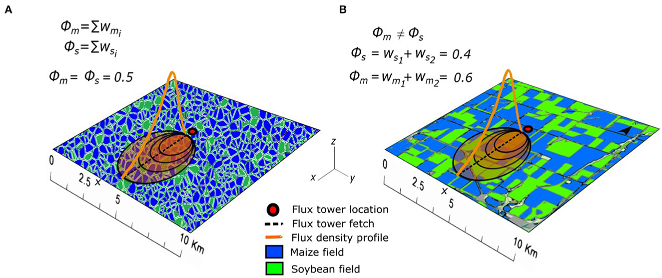
Figure 4. Conceptual illustration of the flux footprint responses of (A) a random land cover mosaic where maize and soybean equally contribute to the total observed flux (ϕm = ϕs = 0.5), and (B) an organized heterogeneous land cover mosaic as observed at the study site.
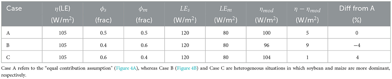
Table 1. Comparison between the random and organized heterogeneous mosaic cases (Figure 4) toward the estimation of latent heat flux, η≡LE.
This example also demonstrates that the change in the relative contribution of fluxes due to two crop species can either increase or decrease the total flux observed at the tower (η) relative to the hypothetical case of a random distribution of crops. In other words, an incremental change in flux observed at a tower could either correlate to a change in flux from the crops or a shift in relative land cover contributions. This has significant implications for flux tower data interpretation in a heterogeneous landscape.
4. Results and discussion
4.1. Flux footprints cover a wide range of landscape areas
The size of the flux footprint strongly depends on the highly variable atmospheric stability at the sub-hourly time scale. At the annual scale or for observations over long periods, the effect of the atmospheric stability on the footprint climatology, an aggregation of footprints over several time steps, is weaker (Kljun et al., 2015; Zhang and Wen, 2015; Tuovinen et al., 2019). The climatological footprint for crop years 2016 (Figure 5A), 2017 (Figure 5B), and 2018 (Figure 5C) show the changes in the average location of the surface source areas, where the outer contour shows the upwind distance (fetch) for the 90% of flux contribution, r90%. Figure 5 illustrates flux footprints under neutral (Figure 5A), unstable (Figure 5C), and, stable (Figure 5E) atmospheric conditions. Turbulent mixing plays an important role in the magnitude of fields' relative contributions, as the weighting of fields farther away from the tower increases with increasing stability. In general, the flux footprint size decreases with decreasing zm/L (Section 3.1). Therefore, under unstable conditions (Figure 5D) we can expect a smaller flux footprint than under stable conditions (Figure 5F). We found that the average distance to the flux footprint peak is 168m for unstable conditions and 268 m for stable conditions (Figure 5G). The footprint is wider as the standard deviation of the lateral wind fluctuations increases and, therefore, the crosswind dispersion increases (Kljun et al., 2015; Zhang and Wen, 2015). On average, the upwind area described by r90% corresponds to 1.51 km2 for unstable conditions and 3.17 km2 under stable conditions. Similarly, the upwind distance to the contour described by the 90% of the flux contribution for unstable conditions is closer than for stable conditions, with 5.8 km and 9.2 km, respectively (Figure 5H). While the 2D flux footprint provides the upwind source area up to a certain percentage of flux contribution, the frequency of the direction and length associated with the prevalent upwind distance for the 90% of contribution (fetch) is not yet known. Here we propose the fetch rose, a graph that shows the frequency of the upwind distance (fetch) from particular directions over a specified period (Figure 6). The fetch roses for crop years 2016 (Figure 6A), 2017 (Figure 6B), and 2018 (Figure 6C) for r90% have a prevalent south-southwest direction in a 16-point compass. While the dominant direction is south-southwest, other wind directions are relatively equiprobable. We see that fetches over 10 km (Figure 6, orange to red) are rare relative to fluxes from 2.5 to 10 km (Figure 6, light blue to yellow) but fetches tend to be at least 2.5 km. We also see that the longest fetches emanate from all directions except north, such that distant fields from the north hardly ever influence tower fluxes. The r90% fetch points toward the prevalent direction 6% of the time on average from 2016 to 2019 (Figure 5D), and its length is 5–7.5km. The implications of these results for partitioning flux contributions for each crop type due to the flux footprint are discussed in the following subsections.
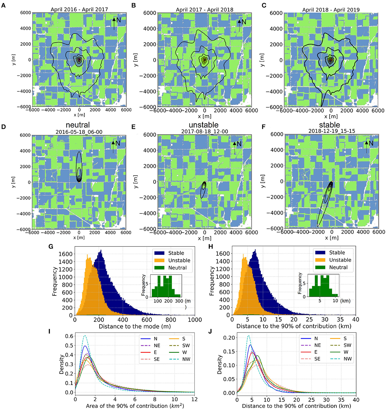
Figure 5. Flux footprint plots with contours over the mosaic of maize (blue) and soybean (green) crops with the center at the flux tower. Each flux footprint plot shows the source area defined by the contours of 20, 40, 60, 80, and 90% (outer contour) of the total flux contribution. The climatological (or average) flux footprint for crop years (A) 2016 (i.e., April 2016 to March 2017), (B) 2017, and (C) 2018, correspond to the aggregation of all single footprints over the year. A sample of single 15-minutes averaged flux footprints under (D) neutral (05/18/2016 06:00), (E) unstable (08/18/2017 12:00), and (F) stable (12/19/2018 15:15) atmospheric conditions show the changes in size and location of the source area of the surface flux defined by the dynamic flux footprint. Histograms of the 15-min FFP analysis for the upwind distance (fetch) to the (G) mode and to the (H) 90% of flux contribution, illustrate the average behavior under stable (blue), unstable (orange), and neutral (green) atmospheric conditions over the 3 years of analysis. The probability density function of the upwind (I) area and (J) distance of the 90% of flux contribution show differences based on wind direction.
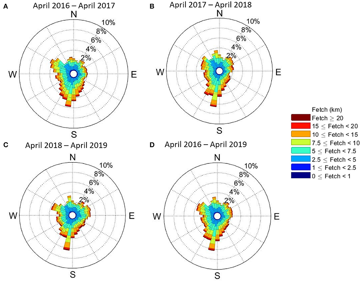
Figure 6. Fetch rose plots show the relative frequency in length and location of the upwind distance (fetch) to the 90% of flux contribution for crop years (A) 2016 (i.e., April 2016 to March 2017), (B) 2017, (C) 2018, and (D) for April 2016 to March 2019. We keep a fixed 15% maximum frequency to compare the prevalent direction and frequencies across crop years. Using a polar coordinate gridding system, the fetch rose shows the frequency over a time period by wind direction with color bands showing fetch ranges. The direction of the longest spoke shows the direction of the upwind distance with the greatest frequency. The concentric circles are used to estimate the relative frequency of the fetch ranges. The fetch rose comprises 4 or more radiating spokes that represent cardinal wind directions, such as the 16-point compass fetch roses presented here. The fetch rose diagram is based on a wind-rose tool (Pereira, 2022) and the fetch for r90% of flux contribution (Kljun et al., 2015).
4.2. Flux contributions evolve due to organized heterogeneity and hydroclimatological drivers
We estimated the relative contribution of average daily fluxes of maize and soybean (Figure 7) using the observed flux tower data. LE, H, and Fc exhibit strong seasonality, where LE and H typically peak between June-August, and Fc is negative during these times, indicating the predominance of photosynthesis over respiration. LE is always high relative to H, indicating that a greater portion of available energy returns to the atmosphere as evapotranspiration instead of a temperature change. Maize dominates in 2016 and 2018, and soybean dominates in 2017, which matches with Figure 5 maps, where most contours cover maize around the tower in 2016 and 2018. However, 2018 has the evenest distribution (e.g., time windows 16–21 for LE), and some time windows (16, a, b) have a dominant soybean influence on LE and H, which might correspond to a prevalence of distant soybean fields planted in the SW direction, even though maize is planted in nearby fields. In terms of flux footprint contribution, ϕ (Figure 7D), a larger contribution from maize fields was observed in 2016 and 2018 when more fields were cultivated with maize in areas between 168 m and 268 m upwind from the tower. In 2017, soybean was mostly planted in the same fields. However, both crop types influence the magnitude of the observed fluxes. In terms of Fc behavior across seasons, we observe that a strong release of CO2 flux, on the order of 2 into the atmosphere occurs during planting (Figure 7C, numerals 1, 9, and 17). This is followed by a much larger uptake of CO2, of approximately 4 , during the following two 6-week windows. This can be explained by rising temperatures and soil moisture that support heterotrophic respiration of existing biomass on and in the soil. Agricultural practices that vary among fields, such as spring tilling, can also spur soil respiration. During the peak of the growing season, soybean fields in 2017 contributed more toward a higher CO2 uptake (Figure 7C, numeral 11), which suggests that soybean fields may be more effective for carbon sequestration, while maize fields in 2016 and 2018 contributed more toward a higher LE (Figure 7C, numeral 2 and 18), which could be attributed to factors such as high temperatures or soil moisture deficits. Accordingly, this 6-week window analysis shows that maize fields inside the flux footprint contributed more toward daily LE and H than soybean fields during the 2016 and 2018 growing seasons, whereas soybean contributed more than maize in 2017. In 2018 however, we note that the contributions are the most similar between the two crop types (Figure 7D), where the prevalent wind direction can cause the footprint to be composed of patches with a more equal distribution of crop types (Figure 6C).
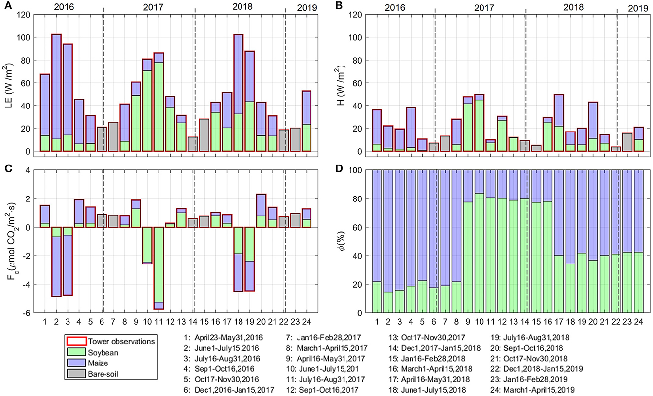
Figure 7. Seasonal evolution of average daily fluxes due to the relative contribution of maize (blue) and soybean (green) in 6-week windows, for (A) latent heat flux, LE; (B) sensible heat flux, H; (C) carbon dioxide flux, Fc; and (D) relative flux footprint contribution, ϕ. Each stacked bar refers to a 6-week average daily flux for each crop type. Dash vertical lines show the years of analysis. The relative contributions due to soybean and maize were calculated with the method described in Section 3 using 15-minute data, from April 2016 to April 2019.
Next, we explore the seasonal dominance of a given crop type in terms of the relative flux footprint contribution in magnitude, ϕ, rather than area contribution. We calculated the difference in the percentage of contribution for the two cases described in Section 3.4. First, for the hypothetical randomly distributed mix of plants, in a manner that does not reflect any particular spatial pattern, where the relative contribution of the flux footprint for each crop type is equal, ϕm = ϕs = 50%. We compare this hypothetical random distribution to the observed contributions of each crop, where ϕm and ϕs are temporally variable and one crop type tends to dominate the footprint contributions. Specifically, the maximum values for ϕm and ϕs are greater than 0.8 (Figure 7). In other words, we want to find what crop is dominant in each window resulting from a combination of fluxes associated with each crop and the fraction they occupy in the flux footprint. To estimate the contribution percentage of each crop, we first calculated the average LE, H, and Fc for maize and soybean for the 6-week windows, using Equations (5)–(7) and the corresponding ϕ for each case. Then, we subtracted the results assuming a random (rather than organized) distribution of crops from the heterogeneous results (i.e., organized heterogeneity), to define the dominant crop for each window. The 6-week averaged analysis shows the difference between the percentage of the contributions for the organized heterogeneous mosaic and for the hypothetical random contribution case (Figure 8). While maize fields contributed more to the observed LE and H in crop years 2016 and 2018, soybean fields contributed more in the crop year 2017 (Figures 8A, B). The largest contribution due to the land cover heterogeneity is observed for CO2 flux (Fc) from June 1 to July 15, 2017 (Figure 8C, bar 10), when on an average soybean fields contribution toward Fc is 24.5% larger than the random case (Figure 8C).
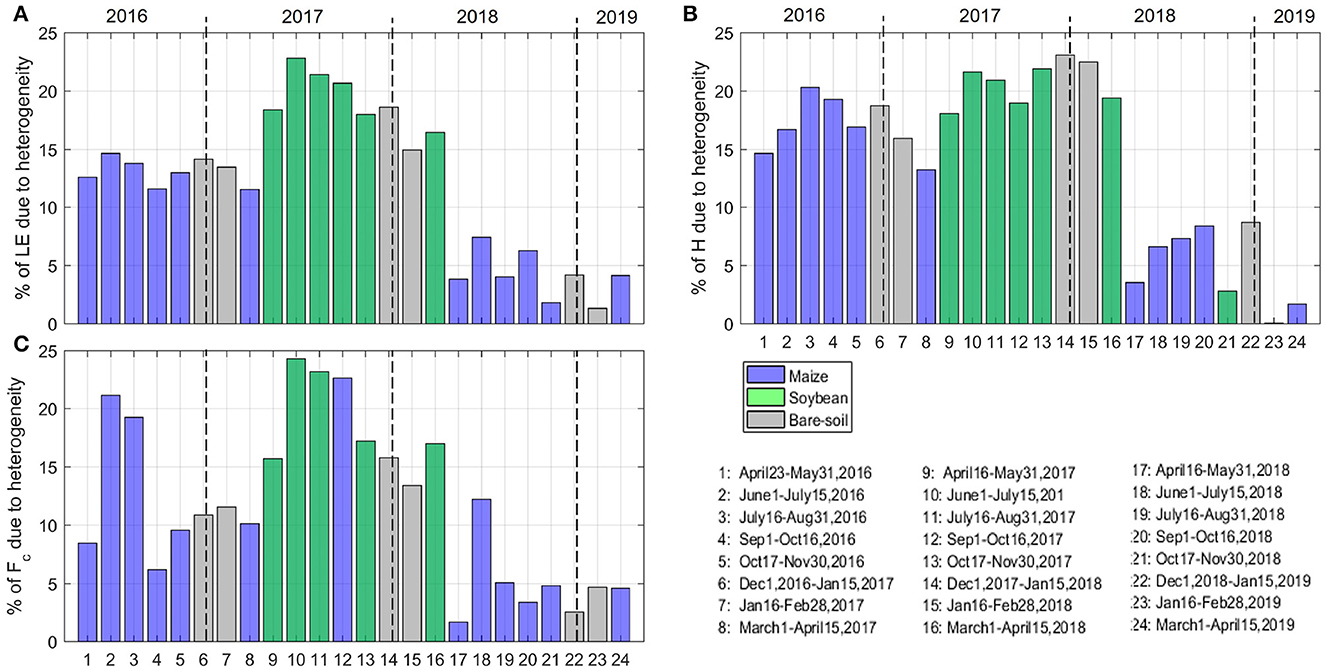
Figure 8. Seasonal evolution of the percent contribution due to organized heterogeneity in 6-week windows, for (A) latent heat flux, LE; (B) sensible heat flux, H; and (C) carbon dioxide flux, Fc. These plots show the difference between the response of a heterogeneous land cover mosaic and a hypothetical random assumption where ϕm = ϕs = 0.5. Dash vertical lines show the years of analysis.
Given that changes in flux observed at the tower could either correlate to a change in flux from the crops or a shift in relative land cover contributions, we analyze the latter based on atmospheric stability conditions and the significance of the contributing areas (Figure 9). Besides the overall high contribution due to maize and soybean areas nearby the tower under unstable conditions, maize and soybean show a different cumulative distribution function based on stability (Figure 9A). Particularly under unstable conditions, the flux footprint is smaller, and therefore there is a higher probability of observing a single crop type (Figure 9A). However, ϕ is always less than 100%, meaning that the contribution comes from a mix of maize and soybean fields (Figure 9B). During 2016–2019 and for unstable conditions, is more likely for ϕm and ϕs to greatly differ (e.g., phis <10% and phim>85%) (Figure 9B). Our results show that stable conditions tend to homogenize the relative percentage of contribution of the two crop types. Therefore, under stable conditions the probability to see large differences between ϕs and ϕm decreases.
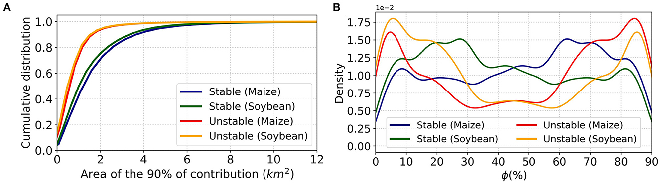
Figure 9. Seasonal behavior of the relative flux footprint contributions due to maize and soybean fields from 2016 to 2019. The cumulative distribution of the (A) area of 90% of flux footprint contribution and the (B) probability density curves of relative flux footprint contributions (ϕ) show the behavior of each crop type under stable (blue and green, for maize and soybean, respectively) and unstable (red and orange, for maize and soybean, respectively) atmospheric conditions.
Although the main purpose of this study is not to validate our modeling results against flux observations but to merge flux tower observations with ecohydrological and flux footprint modeling to improve the crop-specific estimates, we show here that our modeling results of daily averaged fluxes for the 6-week windows of analysis capture the seasonal behavior of the observations for Fc and LE (Figures 10A, B, respectively). In Figure 10, we include metrics that provide some quantitative information about the goodness of fit of observed and modeled results for the daily averaged data for the 6-week windows analysis, such as the Mean Absolute Error (MAE), the Root Mean Squared Error (RMSE), the Mean Squared Error (MSE) and the Normalized Root Mean Squared Error (NRMSE). MAE shows the average magnitude of the difference between the observed and modeled results, in units of the variable being measured. The RMSE and MSE estimate the overall accuracy of the model across the range of the observed results, while the NRMSE provides a normalized measure of the RMSE, taking into account the range of the observed results. We observe a better fit of the observed and modeled data comparison for Fc than for LE across metrics, with Fc having a lower MAE of 0.7 and a lower NRMSE of 0.13, compared to LE which had an MAE of 11.42 and an NRMSE of 0.16. While modeling results tend to slightly overestimate positive Fc during non-growing seasons and match the overall negative Fc observed during the growing seasons, we consider that these results are satisfactory for our purposes given the complexity of the processes involved and the assumptions taken in order to estimate the role played by the land cover heterogeneity on the dynamics of the observed fluxes. If our main purpose were to replicate eddy covariance observations at finer temporal scales using a physically-based modeling approach, more processes and sources of variability would need to be considered besides the crop type influence studied here.
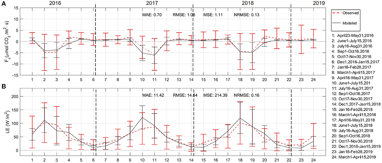
Figure 10. Differences between flux tower observations (red) and modeled (gray) daily averaged fluxes in 6-week windows, for (A) carbon dioxide flux, Fc, and (B) latent heat flux, LE. The error bars show the standard deviation of the daily average over the 6-week period for the observed (red) and modeled data (gray). The segmented line in red shows the behavior of the daily averaged observations, while the continuous black line similarly shows the modeled data. Dashed vertical lines show the years of analysis. The Mean Absolute Error (MAE), Root Mean Squared Error (RMSE), Mean Squared Error (MSE), and Normalized Root Mean Squared Error (NRMSE), support the evaluation of the goodness of fit between observed and modeled data.
4.3. Organized heterogeneity and hydroclimatological drivers explain high 2017 CO2 uptake
Here we use the results of the relative contribution analysis to determine the relationship between the lowest crop yield and the largest net CO2 budget observed in 2017, in comparison to 2016 and 2018. The USDA provides crop yields at the county scale for Piatt county, Illinois (NASS, 2018) (Figure 11A), which we assume is representative of yields at the study site. Here we determine how the different contributions of maize and soybean inside the flux footprint can inform the observations. Explicit dependence on the distance of the contributions from different patches is considered. From MLCan we obtain the net CO2 budget for each crop type during the growing seasons (Figure 11B). Assuming that the CO2 taken up is only used to produce dry matter (DM) and that the weight per bushel of DM for maize is 25.4 Kg/bushel and 27.2 Kg/bushel for soybean (Murphy, 1981), we estimate the net CO2 budget per unit yield for each crop type. We make the simplifying assumption that the CO2 taken up by plants is only used to produce dry matter, and we did not consider any potential changes in soil carbon storage. We acknowledge that this assumption may not fully reflect the complex interactions between plants and soil, where changes in soil carbon storage could potentially influence the carbon balance. Therefore, we provide a rough estimate of the CO2 emissions or sequestration on a carbon basis. We assume a carbon content of 45% for soybean and maize dry matter and converted the kg CO2 / kg dry matter to kg CO2 / kg carbon, which represents the amount of CO2 sequestered per unit of carbon contained in the crops (Figure 11C). Given that the net CO2 during the growing season is negative, more CO2 is taken up than released. The carbon sequestered, which is measured kg CO2/kg C, and calculated by:
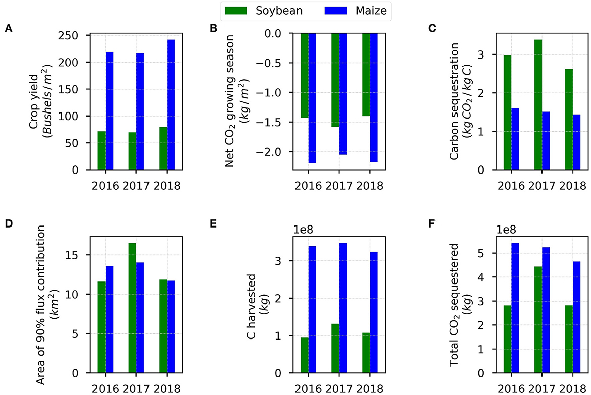
Figure 11. Relationship between crop yield, net CO2 during the growing season, and emissions or sequestration on a carbon basis. (A) Crop yields at Piatt county are combined with (B) the net CO2 budget for each crop type during the growing seasons 2016–2018 estimated with MLCan, to calculate (C) the carbon sequestered for soybean and maize. (D) The climatological flux footprint area for the 90% contribution is used to calculate (E) a broad estimate of the amount of carbon that is harvested and (F) of the amount of CO2 sequestered by each crop inside the flux footprint.
This provides a way to compare the carbon impact of soybean and maize, and we observe that soybean has a larger CO2 uptake than maize (Figure 11C). By using the area of the average 90% flux contribution using the climatological flux footprint (Figure 11D), we can provide a broad estimate of the amount of carbon that is harvested from each crop within the flux footprint (Figure 11E):
To estimate the total amount of CO2 sequestered by each crop inside the flux footprint, we multiply the amount of carbon harvested by the kg CO2/kg carbon value for each crop (Figure 11F). Both the C harvested and CO2 inside the flux footprint are larger for maize than for soybean across years, and the highest C harvested and CO2 uptake from soybean fields occurred in 2017 (Figures 11E, F). Given that soybean fields take up more CO2, even in a drier, low-yield year, we see more CO2 uptake for a year in which soybean is dominant inside the footprint; Figure 11D). Also, CO2 release is muted from respiration by the drier conditions, further skewing the net flux toward high CO2 uptake. Therefore, we observe that the higher annual net CO2 budget in the crop year 2017 is not only the effect of hydroclimatological conditions but the particular contribution of soybean fields, which play a significant role in the higher uptake of CO2 observed that year. The combination of CO2 taken up by soybean fields and the drying that occurs due to the high temperatures and lower rainfall, influence the overall higher uptake of CO2 observed in 2017. These results show how multiple sources besides the observed Fc (i.e., MLCan and flux footprint modeling, as well as crop yield data), provide elements for an informed interpretation of the influence of the organized land cover heterogeneity on the behavior of observed land-atmosphere fluxes.
5. Summary and conclusions
This study illustrates the important role of the organized land cover heterogeneity on the observed land-atmosphere fluxes of heat, water, and CO2, where the observations come from a flux tower that sees the intensively managed agricultural landscape, instead of a single crop field. When the land cover is heterogeneous, inconsistencies in data interpretation can arise when only accounting for the vegetation type in the nearest field, or alternatively assuming that multiple crop types contribute equally to the observed flux. Area weighting based on the relative distribution of crop areas will not work as the fractional contribution from each crop changes with the dynamically changing flux footprint. Therefore, our framework combines flux footprint and ecohydrological modeling with flux tower data to improve upon the understanding that could be obtained given any single information source. The observations reflect the predominance of the crop fields within the flux footprint and we determine their fractional weighted contributions to the observed value resulting from the proximity to the tower.
Our approach to analyzing the relative flux contributions has some limitations, many of which could be improved upon in future studies. First, we consider that crops and soil components are the primary sources of CO2 and that extremely low traffic in the nearby farm roads and other local sources are negligible contributors (the flux tower is strategically located away from major highways). Determining the precise contribution of automobile and mechanized farm equipment emissions to observed CO2 fluxes is a challenging task. However, we assume that such emissions are likely to have a negligible impact over our 6-week observation periods. Although there may be a few days during the planting or harvesting seasons when there is a significant activity within parts of the flux footprint, the impact of this activity is relatively small when averaged over all time points. For example, even if there were significant farm work going on for 40-time steps during a six-week window, out of a total of 4,032-time steps, the impact of this activity would be minimal, even if the CO2 flux was doubled during those time steps. Similarly, the contribution of traffic on country roads to the observed CO2 flux is expected to be negligible when averaged over a long period, given that most of the roads are rural or far from the tower. Second, the estimation of the flux footprint is not the only source of error, since tower observations and the ecohydrological model also have errors and as a result, they contribute some uncertainty to our estimations. Third, we do not consider the variability in flux response across multiple fields cultivated with the same crop, but we assume a representative modeled flux. Specifically, we distinguish between “maize” or “soybean” patches and ignore other differentiating factors. In reality, all maize or soybean fields may not behave the same due to differences in cultivars, soil type, microtopographic variability, time of planting, etc. This assumption can be overcome through a distributed modeling approach if detailed data to support such modeling is available. For example, given a detailed map of soil texture or topography, the landscape could be divided into more than two components that could be modeled and attributed at higher resolution. Meanwhile, landscape attributes within the flux footprint may be correlated with meteorological conditions that define the footprint itself. In this case, it is challenging to disentangle the influence of landscape heterogeneity versus weather variables that also shift with wind direction. Further analysis can include the implementation of the fetch rose for different stability conditions. The fetch rose can provide a further look into the spatial distribution of the contributing plots to match areas of “well-drained maize” or “drier soybean” enabling testing of the assumption that vegetation type is the dominant differentiating factor between fluxes at different landscape patches. We anticipate that our study could be extended to study other natural and human-induced interventions on heterogeneous agricultural landscapes, such as varying wetness conditions, LAI, or planting dates, or for comparison with a remote sensing product. However, specifying spatially variable precipitation at these resolutions could remain a formidable challenge. This approach could also be applied to model evaluation, in that the representation of landscape heterogeneity should lead to an improved agreement between model results and observations, relative to the assumption that the tower measurements represent a single crop type or a homogeneous contribution from multiple crop types. In general, our method is relevant for the understanding of land-atmosphere fluxes in heterogeneous landscapes and can be extended toward the use of flux tower data as validation for models of these fluxes.
Our analyses show that the fluxes observed at the 25 m tall flux tower are the result of the combined action of (1) hydroclimatological drivers acting on the ecosystem, and (2) the difference in the fraction of maize and soybean in the flux footprint due to the organized heterogeneity of the land cover. In other words, the change in the flux observed at every time step (15 min) could either correlate to a change in flux from the crops or a shift in relative land cover contributions within the footprint due to wind, or both. For instance, we qualitatively demonstrated that the change in the relative contribution of fluxes due to two different land cover types can either increase or decrease the total flux observed at the tower. Therefore, we quantitatively showed that the spatial structure of the land cover, described here as “organized land cover heterogeneity” and characterized by the mosaic of crop fields, impacts the observed fluxes. Our focus on the relative contribution of maize and soybean fields inside the flux footprint shows the importance of an accurate description of the land cover and the use of an accurate flux footprint method. We recognize that it is equally important to accurately simulate the flux response of each vegetation species under the observed atmospheric drivers. All these are used to obtain the variability of the areal coverage and the temporal variability of the flux.
In an intensively managed agricultural landscape, where each land cover patch is easily identifiable by crop type (i.e., maize or soybean), we quantified the relative flux contribution of LE, H, and CO2. At the study site, the cultivated fields where the flux contribution peaks are mainly due to one crop type, which explains the dominance in fluxes contribution given by maize-soybean-maize for the 2016–2017–2018 crop years, respectively. This combined analysis makes it feasible to investigate questions regarding real and hypothetical land cover changes at an ecosystem scale and quantify the effects of different vegetation types on ecosystem fluxes.
Data availability statement
The two-dimensional Flux Footprint Prediction (FFP) model used in this study is available at https://footprint.kljun.net/ (Kljun et al., 2015). MLCan2.0 model (Drewry et al., 2010; Le et al., 2012) and datasets used in this study are publicly available on GitHub (https://github.com/HydroComplexity/MLCan2.0/tree/master/Data/Goose_Creek and https://doi.org/10.5281/zenodo.3931001).
Author contributions
LH, AG, and PK conceptualized and designed the study and contributed to the revision of the manuscript. LH performed the numerical simulations, developed the initial draft, and developed the concept of the Fetch Rose. All authors contributed to the article and approved the submitted version.
Funding
This work was supported by NSF grant EAR-1331906 for the Critical Zone Observatory for Intensively Managed Landscapes (IMLCZO), a multi-institutional collaborative effort, NSF grant OAC-1835834, and NSF grant EAR-2012850 for the Critical Interface Network for Intensively Managed Landscapes (CINet). AG is partially supported by NASA New Investigator Program Award 80NSSC21K0934.
Acknowledgments
We thank Steve Sargent at the Illinois State Geological Survey for supporting the data collection from the flux tower.
Conflict of interest
The authors declare that the research was conducted in the absence of any commercial or financial relationships that could be construed as a potential conflict of interest.
Publisher's note
All claims expressed in this article are solely those of the authors and do not necessarily represent those of their affiliated organizations, or those of the publisher, the editors and the reviewers. Any product that may be evaluated in this article, or claim that may be made by its manufacturer, is not guaranteed or endorsed by the publisher.
Supplementary material
The Supplementary Material for this article can be found online at: https://www.frontiersin.org/articles/10.3389/frwa.2023.1033973/full#supplementary-material
References
Alekseychik, P., Korrensalo, A., Mammarella, I., Vesala, T., and Tuittila, E.-S. (2017). Relationship between aerodynamic roughness length and bulk sedge leaf area index in a mixed-species boreal mire complex. Geophys. Res. Lett. 44, 5836–5843. doi: 10.1002/2017GL073884
Alfieri, J. G., Kustas, W. P., Prueger, J. H., Hipps, L. E., Evett, S. R., Basara, J. B., et al. (2012). On the discrepancy between eddy covariance and lysimetry-based surface flux measurements under strongly advective conditions. The Bushland Evapotranspiration and Agricultural Remote Sensing Experiment 2008. Adv. Water Resour. 50, 62–78. doi: 10.1016/j.advwatres.2012.07.008
Anders, A. M., Bettis III, E. A., Grimley, D. A., Stumpf, A. J., and Kumar, P. (2018). Impacts of quaternary history on critical zone structure and processes: examples and a conceptual model from the Intensively Managed Landscapes Critical Zone Observatory. Front. Earth Sci. 6, 24. doi: 10.3389/feart.2018.00024
Aubinet, M., Vesala, T., and Papale, D. (2012). Eddy Covariance: A Practical Guide to Measurement and Data Analysis. Berlin: Springer Science Business Media. doi: 10.1007/978-94-007-2351-1
Biermann, T., Babel, W., Ma, W., Chen, X., Thiem, E., Ma, Y., et al. (2014). Turbulent flux observations and modelling over a shallow lake and a wet grassland in the nam co basin, Tibetan Plateau. Theoret. Appl. Climatol. 116, 301–316. doi: 10.1007/s00704-013-0953-6
Burba, G. (2013). Eddy Covariance Method for Scientific, Industrial, Agricultural and Regulatory Applications: A Field Book on Measuring Ecosystem Gas Exchange and Areal Emission Rates. Lincoln, NE: LI-Cor Biosciences.
Chi, J., Nilsson, M. B., Kljun, N., Wallerman, J., Fransson, J. E., Laudon, H., et al. (2019). The carbon balance of a managed boreal landscape measured from a tall tower in northern Sweden. Agric. For. Meteorol. 274, 29–41. doi: 10.1016/j.agrformet.2019.04.010
Chi, J., Nilsson, M. B., Laudon, H., Lindroth, A., Wallerman, J., Fransson, J. E. S., et al. (2020). The net landscape carbon balance-integrating terrestrial and aquatic carbon fluxes in a managed boreal forest landscape in Sweden. Glob. Change Biol. 26, 2353–2367. doi: 10.1111/gcb.14983
Chu, H., Luo, X., Ouyang, Z., Chan, W. S., Dengel, S., Biraud, S. C., et al. (2021). Representativeness of eddy-covariance flux footprints for areas surrounding ameriflux sites. Agric. For. Meteorol. 301, 108350. doi: 10.1016/j.agrformet.2021.108350
Drewry, D., Kumar, P., Long, S., Bernacchi, C., Liang, X.-Z., and Sivapalan, M. (2010). Ecohydrological responses of dense canopies to environmental variability: 1. Interplay between vertical structure and photosynthetic pathway. J. Geophys. Res. Biogeosci. 115, G4. doi: 10.1029/2010JG001340
ECMWF (2018). Era5 Hourly Data on Single Levels From 1979 to Present. Fifth Generation of ECMWF Atmospheric Reanalyses of the Global Climate. ECMWF. Available online at: https://cds.climate.copernicus.eu/cdsapp#!/dataset/reanalysis-era5-single-levels?tab=form (accessed January 4, 2021).
Foken, T. (2006). 50 years of the monin-obukhov similarity theory. Boundary-Layer Meteorol. 119, 431–447. doi: 10.1007/s10546-006-9048-6
Foufoula-Georgiou, E., Takbiri, Z., Czuba, J. A., and Schwenk, J. (2015). The change of nature and the nature of change in agricultural landscapes: hydrologic regime shifts modulate ecological transitions. Water Resourc. Res. 51, 6649–6671. doi: 10.1002/2015WR017637
Gao, S., Niu, Z., Huang, N., and Hou, X. (2013). Estimating the leaf area index, height and biomass of maize using hj-1 and radarsat-2. Int. J. Appl. Earth Observ. Geoinform. 24, 1–8. doi: 10.1016/j.jag.2013.02.002
Horst, T., and Weil, J. (1992). Footprint estimation for scalar flux measurements in the atmospheric surface layer. Boundary-Layer Meteorol. 59, 279–296. doi: 10.1007/BF00119817
Jacobs, A. F., and Van Boxel, J. H. (1988). Changes of the displacement height and roughness length of maize during a growing season. Agric. For. Meteorol. 42, 53–62. doi: 10.1016/0168-1923(88)90066-4
Kirby, S., Dobosy, R., Williamson, D., and Dumas, E. (2008). An aircraft-based data analysis method for discerning individual fluxes in a heterogeneous agricultural landscape. Agric. For. Meteorol. 148, 481–489. doi: 10.1016/j.agrformet.2007.10.011
Kljun, N., Calanca, P., Rotach, M., and Schmid, H. P. (2015). A simple two-dimensional parameterisation for flux footprint prediction (FFP). Geosci. Model Dev. 8, 3695–3713. doi: 10.5194/gmd-8-3695-2015
Kumar, P., Le, P. V., Papanicolaou, A. T., Rhoads, B. L., Anders, A. M., Stumpf, A., et al. (2018). Critical transition in critical zone of intensively managed landscapes. Anthropocene 22, 10–19. doi: 10.1016/j.ancene.2018.04.002
Le, P. V., and Kumar, P. (2014). Power law scaling of topographic depressions and their hydrologic connectivity. Geophys. Res. Lett. 41, 1553–1559. doi: 10.1002/2013GL059114
Le, P. V., Kumar, P., Drewry, D. T., and Quijano, J. C. (2012). A graphical user interface for numerical modeling of acclimation responses of vegetation to climate change. Comput. Geosci. 49, 91–101. doi: 10.1016/j.cageo.2012.07.007
Leclerc, M. Y., and Foken, T. (2014). Footprints in Micrometeorology and Ecology Volume 239. Berlin: Springer. doi: 10.1007/978-3-642-54545-0
Lee, T. R., and De Wekker, S. F. (2016). Estimating daytime planetary boundary layer heights over a valley from rawinsonde observations at a nearby airport: an application to the page valley in virginia, united states. J. Appl. Meteorol. Climatol. 55, 791–809. doi: 10.1175/JAMC-D-15-0300.1
Licor (2021). Tovi. Available online at: https://licor.com/tovi/ (accessed August 13, 2021).
Masson-Delmotte, V., Arias, P., Bellouin, N., Coppola, E., Jones, R., Krinner, G., et al. (2021). IPCC, 2021: Climate Change 2021: The Physical Science Basis. Contribution of Working Group I to the Sixth Assessment Report of the Intergovernmental Panel on Climate Change. Cambridge: Cambridge University Press.
Mishra, V., and Cherkauer, K. A. (2010). Retrospective droughts in the crop growing season: implications to corn and soybean yield in the Midwestern United States. Agric. For. Meteorol. 150, 1030–1045. doi: 10.1016/j.agrformet.2010.04.002
Monfreda, C., Ramankutty, N., and Foley, J. A. (2008). Farming the planet: 2. Geographic distribution of crop areas, yields, physiological types, and net primary production in the year 2000. Glob. Biogeochem. Cycles 22:GB1022. doi: 10.1029/2007GB002947
Myneni, R., Knyazikhin, Y., and Park, T. (2015). Mod15a2h Modis/Terra Leaf Area Index/fpar 8-Day l4 Global 500 m sin grid v006. NASA EOSDIS Land Processes, DAAC.
NASS U (2016–2018). Illinois corn and Soybean County Estimates. USDA National Agricultural Statistics Service, Illinois County Estimates, Corn and Soybean, 2016–2018.
NASS U (2010). Field Crops: Usual Planting and Harvesting Dates. Agriculural Handbook 628. Washington, DC: USDA National Agricultural Statistics Service.
Nguy-Robertson, A., Gitelson, A., Peng, Y., Vina, A., Arkebauer, T., and Rundquist, D. (2012). Green leaf area index estimation in maize and soybean: combining vegetation indices to achieve maximal sensitivity. Agron. J. 104, 1336–1347. doi: 10.2134/agronj2012.0065
Pereira, D. (2022). Wind Rose. Available online at: https://www.mathworks.com/matlabcentral/fileexchange/47248-wind-rose (accessed August 18, 2022).
Richardson, M., and Kumar, P. (2017). Critical zone services as environmental assessment criteria in intensively managed landscapes. Earth's Fut. 5, 617–632. doi: 10.1002/2016EF000517
Schmid, H. (1994). Source areas for scalars and scalar fluxes. Boundary-Layer Meteorol. 67, 293–318. doi: 10.1007/BF00713146
Schuepp, P., Leclerc, M., MacPherson, J., and Desjardins, R. (1990). Footprint prediction of scalar fluxes from analytical solutions of the diffusion equation. Boundary-Layer Meteorol. 50, 355–373. doi: 10.1007/BF00120530
Seidel, D. J., Zhang, Y., Beljaars, A., Golaz, J.-C., Jacobson, A. R., and Medeiros, B. (2012). Climatology of the planetary boundary layer over the continental United States and Europe. J. Geophys. Res. Atmos. 117, D16. doi: 10.1029/2012JD018143
Stull, R. B. (2012). An Introduction to Boundary Layer Meteorology Volume 13. Springer Science and Business Media.
Tuovinen, J.-P., Aurela, M., Hatakka, J., Räsänen, A., Virtanen, T., Mikola, J., et al. (2019). Interpreting eddy covariance data from heterogeneous siberian tundra: land-cover-specific methane fluxes and spatial representativeness. Biogeosciences 16, 255–274. doi: 10.5194/bg-16-255-2019
Vesala, T., Kljun, N., Rannik, Ü., Rinne, J., Sogachev, A., Markkanen, T., et al. (2008). Flux and concentration footprint modelling: state of the art. Environ. Pollut. 152, 653–666. doi: 10.1016/j.envpol.2007.06.070
Vitale, D., Bilancia, M., and Papale, D. (2019). Modelling random uncertainty of eddy covariance flux measurements. Stochast. Environ. Res. Risk Assess. 33, 725–746. doi: 10.1007/s00477-019-01664-4
Vogelezang, D., and Holtslag, A. A. (1996). Evaluation and model impacts of alternative boundary-layer height formulations. Boundary-Layer Meteorol. 81, 245–269. doi: 10.1007/BF02430331
Wang, H., Jia, G., Zhang, A., and Miao, C. (2016). Assessment of spatial representativeness of eddy covariance flux data from flux tower to regional grid. Remote Sens. 8, 742. doi: 10.3390/rs8090742
Warner, R. E., Havera, S. P., David, L. M., and Siemers, R. J. (1989). Seasonal abundance of waste corn and soybeans in Illinois. J. Wildl. Manage. 53, 142–148. doi: 10.2307/3801321
Wilson, C. G., Abban, B., Keefer, L. L., Wacha, K., Dermisis, D., Giannopoulos, C., et al. (2018). The intensively managed landscape critical zone observatory: a scientific testbed for understanding critical zone processes in agroecosystems. Vadose Zone J. 17, 1–21. doi: 10.2136/vzj2018.04.0088
Keywords: land cover heterogeneity, eddy covariance, flux footprint, fetch rose, flux partitioning, ecohydrological modeling, critical zone science, intensively managed landscapes
Citation: Hernandez Rodriguez LC, Goodwell AE and Kumar P (2023) Inside the flux footprint: The role of organized land cover heterogeneity on the dynamics of observed land-atmosphere exchange fluxes. Front. Water 5:1033973. doi: 10.3389/frwa.2023.1033973
Received: 01 September 2022; Accepted: 15 March 2023;
Published: 31 March 2023.
Edited by:
Erin Seybold, University of Kansas, United StatesReviewed by:
Mark Potosnak, DePaul University, United StatesXiaofan Yang, Beijing Normal University, China
Copyright © 2023 Hernandez Rodriguez, Goodwell and Kumar. This is an open-access article distributed under the terms of the Creative Commons Attribution License (CC BY). The use, distribution or reproduction in other forums is permitted, provided the original author(s) and the copyright owner(s) are credited and that the original publication in this journal is cited, in accordance with accepted academic practice. No use, distribution or reproduction is permitted which does not comply with these terms.
*Correspondence: Leila C. Hernandez Rodriguez, bGNoZXJuYW5kZXpyb2RyaWd1ZXpAbGJsLmdvdg==
†Present address: Leila C. Hernandez Rodriguez, Lawrence Berkeley National Laboratory, Berkeley, CA, United States