Investigation of hydrometeorological influences on reservoir releases using explainable machine learning methods

Long short-term memory (LSTM) networks have demonstrated successful applications in accurately and efficiently predicting reservoir releases from hydrometeorological drivers including reservoir storage, inflow, precipitation, and temperature. However, due to its black-box nature and lack of process-based implementation, we are unsure whether LSTM makes good predictions for the right reasons. In this work, we use an explainable machine learning (ML) method, called SHapley Additive exPlanations (SHAP), to evaluate the variable importance and variable-wise temporal importance in the LSTM model prediction. In application to 30 reservoirs over the Upper Colorado River Basin, United States, we show that LSTM can accurately predict the reservoir releases with NSE ≥ 0.69 for all the considered reservoirs despite of their diverse storage sizes, functionality, elevations, etc. Additionally, SHAP indicates that storage and inflow are more influential than precipitation and temperature. Moreover, the storage and inflow show a relatively long-term influence on the release up to 7 days and this influence decreases as the lag time increases for most reservoirs. These findings from SHAP are consistent with our physical understanding. However, in a few reservoirs, SHAP gives some temporal importances that are difficult to interpret from a hydrological point of view, probably because of its ignorance of the variable interactions. SHAP is a useful tool for black-box ML model explanations, but the hydrological processes inferred from its results should be interpreted cautiously. More investigations of SHAP and its applications in hydrological modeling is needed and will be pursued in our future study.

1. Introduction

Reservoirs are natural or human-built lakes that are designed to collect, store, and release water through water infrastructures such as dams in a timely manner. The capability of managing water resources allows reservoirs to serve multiple functions, including municipal and industrial water consumption, hydropower generation, agricultural irrigation, ecosystem productivity, flood and drought protection, and recreation (Yang et al., 2021; Zhang D. et al., 2022). Furthermore, the reservoir water quality also plays important roles in controlling the health of aquatic ecosystems and impacting drinking water resources and human health (Duan et al., 2013, 2015, 2016). Thus, accurate and timely forecast of the reservoir's daily release is imperative for economic development, environmental protection, and our nation's security (Yang et al., 2016, 2020). Because of complex engineering conditions and natural environment are intertwined in the reservoir's operations and functions, reservoir release decisions are affected by many hydrological factors, such as the reservoir storage and inflow. In recent years, climate change and hydrological intensification have resulted in more frequent and intensive natural hazards, such as heavy rainfall, severe flooding, and extreme heat (Fan et al., 2022a). Therefore, the meteorological and climate forcing play more and more important roles in affecting the reservoir release decisions (Ehsani et al., 2017; Yang et al., 2017).

Since the time series observations such as inflow and storage contain both natural factors and human operating management experience, data-driven ML models have been increasingly being applied in assist of the reservoir management (Chang et al., 2016; Liu et al., 2017, 2019; Bozorg-Haddad et al., 2018; Uysal et al., 2018; Niu et al., 2019; Zolfaghari and Golabi, 2021). Many studies have explored the applicability of using the linear regression models (e.g., ridge and lasso regressions) and decision trees-based models (e.g., random forest, extreme gradient boosting tree) to forecast the controlled reservoir releases (Zhang et al., 2018; Rahnamay Naeini et al., 2020; Yang et al., 2021). In these ML models, the interpretation of the prediction is straightforward because these models have a transparent process and internal logic to allow end-users to understand the mathematical mapping from inputs to outputs. For example, we can use the weight in a linear regression model to directly evaluate the relative importance of a feature on the model prediction. In a decision tree-based model, the interpretation of a prediction for an instance can be directly visualized through the graphical presentation and the relative importance of a feature in the prediction depends on the distance to the root node of the tree. However, these ML models are incapable of directly taking the temporal dependence into consideration if the inputs and outputs are time series observations, resulting in a less accurate prediction accuracy.

Long short-term memory (LSTM) networks (a variant of recurrent neural network), take sequence data as inputs, and support multiple parallel input sequences for multivariate inputs, which enable it to effectively extract the information from inputs within previous time steps, capture the temporal dependencies between variables, and efficiently learn the relationship between the multi-inputs and reservoir release (Yu et al., 2019; Lu et al., 2021). Several studies have demonstrated promising results in applying LSTM networks to predict the controlled reservoir release from historical data, analyze the influencing factors, learn the operation rules, and assist reservoir release decision making (Zhang et al., 2018, 2019; García-Feal et al., 2022). However, because of LSTM's recurrent structure and unique gating mechanisms, the internal signals embedded in LSTM networks in terms of states and gates demonstrate complex and interdependent features. With this level of complexity, it is difficult to interpret the variable importance and the variable-wise temporal importance on the model prediction. Furthermore, LSTM models directly learn the statistical relationship between input variables and output observations, which neglects the physical constraints and mass balance equations. Thus, despite the potential advantages of accurately and efficiently simulating the reservoir release, the lack of transparency of LSTM networks and process-based implementation impede the reservoir operators to understand the hydrometeorological influences on the reservoir release and make further operation decisions.

Recently, there has been growing emphasis on building explainable ML techniques to improve the comprehensibility of processes being modeled, understand why a model generates a certain prediction, and explore what features are the most important drivers in the prediction (Shen, 2018; Reichstein et al., 2019; Beven, 2020; Jiang et al., 2022; Lees et al., 2022; Lu et al., 2022b). Most prominent of the explainable ML techniques are the post-hoc methods that focus on explaining the output of a complex model in terms of its inputs (Slack et al., 2020, 2021). These methods are usually local, model-agnostic, and do not depend on the underlying models (Murdoch et al., 2019). One popular unified approach to interpret the trained ML models is SHapley Additive exPlanations (SHAP), which is based on optimal Shapley values from the game theory (Lundberg and Lee, 2017). It integrates several existing approaches with a solid theoretical foundation, guaranteeing that there is a unique solution for the measurement of additive feature importance scores (Lundberg and Lee, 2017; Sundararajan and Najmi, 2020; Fryer et al., 2021). SHAP estimates the contribution by each feature to the prediction of a ML model and provides local interpretations through the generation of perturbations of a given instance in the data. While SHAP is an instance-based explainer, we can also obtain global level explanations through aggregations of local explanations (Lundberg et al., 2020).

Several studies have explored the interpretability of ML models using SHAP in hydrology applications. For example, Song et al. (2022) trained the LSTM model for rainfall-discharge processes using previous 1 year's precipitation data at monthly scale from seven meteorological stations and used SHAP to interpret the LSTM model simulations. They found that the spatial-temporal influence of precipitation on the spring discharge prediction based on the SHAP analysis is consistent with the physical hydrology explanation. Lin et al. (2021) used multi-layer perceptron neural networks and LSTM to forecast the hourly streamflow with previous 7 h streamflow and 10 h precipitation observations and then applied SHAP to quantify the contribution of each variable to the ML model prediction. They found that SHAP failed to provide a definite conclusion with respect to the temporal importance of input variables on the streamflow prediction. Yang and Chui (2021) simulated the rainfall-runoff processes of sustainable urban drainage systems at sub-hourly timescales using XGBoost ML model. Despite the high prediction accuracy for the discharge prediction, they found that the inferred hydrological processes are not consistent with the physical realism through the SHAP analysis (e.g., rainfall provides negative contributions to the runoff). Therefore, despite the generality and convenient usage, it is still not clear whether we can use SHAP to interpret the modeling process of ML models and LSTM networks in particular and obtain physically plausible explanations that can correlate the right predictions with the involved hydrological processes.

To this end, we use SHAP to investigate how LSTM makes predictions of reservoir release from hydrometeorological drivers and explore the capability of SHAP to provide reliable and accurate explanations for the hydrological processes being simulated by the LSTM model. Specifically, we build an interpretable deep learning model by coupling the LSTM network and SHAP for daily reservoir release prediction in 30 reservoirs over the Upper Colorado River Basin, United States. We investigate the influence on the reservoir's daily release decisions from hydrometeorological factors including reservoir storage, inflow, precipitation, and temperature, as well as their temporal influences. We believe that this study is an important step to improve the understanding and trust of reservoir release predictions from ML models and assist the reservoir operation and decision-making.

The main contributions of this paper are:

• We apply LSTM networks for predicting reservoir releases based on multiple hydrometeorological inputs and by considering their long-term influence on the released flow.

• We identify the contributions of four hydrometeorological variables and their temporal importance to the reservoir release prediction from the SHAP analysis.

• We explore whether SHAP can provide physically plausible explanations to the hydrological processes being simulated by the LSTM model.

2. Materials and methods

In this section, we first describe the data generation. Next, we introduce the LSTM and SHAP methods. Last, we will describe experimental design, followed by the model evaluation statistics.

2.1. Study area and data

The Upper Colorado River Basin is comprised of four states, including Colorado, New Mexico, Utah, and Wyoming. The vast majority of fresh water contributed to the Colorado River Basin is collected from the Upper Basin States, primarily through winter snowpack and spring runoff. Influenced by climate change, the water availability of the Upper Colorado River Basin faces many challenges from the amount of snowpack in winter, the timing of spring runoff, and the persistent drought. The reservoir systems in the Upper Colorado River Basin provide water supply to nearly 40 million people till 2021 and serve multiple roles in managing water resources, such as hydropower generation, flood control, irrigation, as well as recreational attractions for skiing, fishing, and boating. The reservoir inflow, storage, and release records in the basin can be downloaded from the U.S. Bureau of Reclamation water operation archive (https://www.usbr.gov/rsvrWater/HistoricalApp.html). In this study, we consider 30 reservoirs in the Upper Colorado River Basin based on the criterion that there are no more than 10 days missing data in the record, which may significantly reduce the prediction accuracy within this time period. Figure 1 shows the locations of these 30 reservoirs. They are non-uniformly distributed in the basin with a quite large difference in elevations. Table 1 summarizes the basic information of these 30 reservoirs including their names, data record length, elevation and storage. As we can see, the reservoirs have varying elevations and storage volumes. Also, some reservoirs have a long record of data up to 30 years and some have a relatively short record with only 13 years of data. Moreover, the reservoir features, such as elevation and storage affect the release patterns, which could also affect the prediction performance. We discuss these factors' influence in detail in Section 3.

FIGURE 1

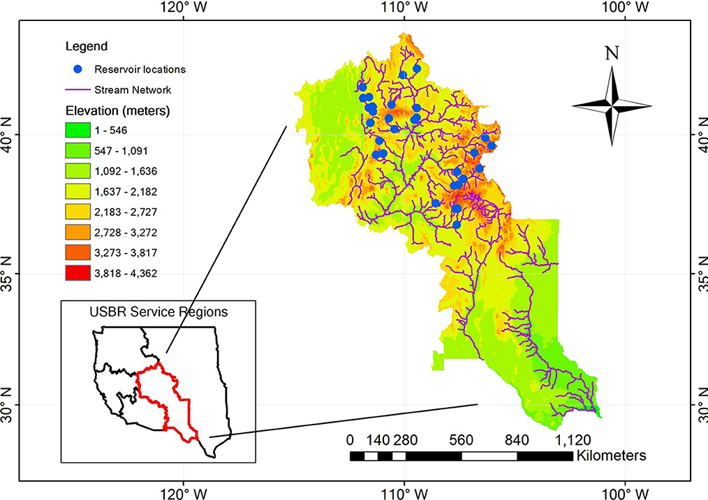
Figure 1. The 30 reservoirs (blue dots) in Upper Colorado River Basin are considered in this study. The figure is modified from Yang et al. (2021).

TABLE 1

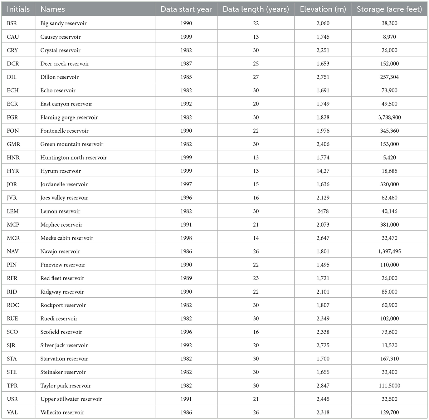
Table 1. The summary of reservoir information for the reservoirs considered in this study.

Besides the hydrological data of inflow and storage, we additionally consider the influence of meteorological data on reservoir releases. The daily average precipitation and temperature data are retrieved from the AN81d dataset generated from Parameter-elevation Regressions on Independent Slopes Model (PRISM). The gridded PRISM has a spatial resolution of 4 km (about 0.04 degrees) and merges surface measurement with an elevation model (Daly and Bryant, 2013). Both PRISM precipitation and temperature data are retrieved from the overlapping pixels of the corresponding study reservoirs in the period between 01/01/1982 and 12/31/2011 to match the reservoir data period listed in Table 1. Considering that the 30 reservoirs have different data lengths on inflow, storage, and release, for each reservoir, we trim the precipitation and temperature data length to match its reservoir data length to ensure these five data sequences have the same periods for the machine learning tasks.

2.2. Model development

In this study, two hydrological variables, reservoir storage S and inflow Q, and two meteorological forcings, precipitation P and Temperature T, are considered as input variables to forecast the reservoir release R. Let random Vector x_k denote previous k days of hydrometeorological observations:

$\begin{array}{l}{\text{x}}_k=[S_{t-1},S_{t-2},...,S_{t-k},\\ Q_{t-1},Q_{t-2},...,Q_{t-k},P_{t-1},P_{t-2},...,P_{t-k},T_{t-1},T_{t-2},...,T_{t-k}]& (1)\end{array}$

It is assumed that the relationship between the multi-inputs and reservoir release can be learned through the ML algorithm from observation data x_k to R_t:

$\begin{array}{ll}{R}_t=f_{\theta }\left({\text{x}}_k\right)& (2)\end{array}$

Where f is a ML function learned by an ML algorithm and θ are parameters of f.

2.3. Long short-term memory network

We use LSTM networks to simulate reservoir releases from hydrometeorological observations and investigate their influences. As a special type of recurrent neural networks, LSTM is structured to learn long-term dependence in time series prediction. In daily reservoir release modeling, we use previous t days of hydrometeorological observations as inputs to predict release on the current day. LSTM learns a mapping for the inputs over time to an output. Thus, it knows what observations it has seen previously are relevant and how they are relevant to the prediction, which enables a dynamical learning of temporal dependence.

The LSTM cell uses four functions and three of them are acting as regulatory gates to control the information flow extracted from the inputs. Furthermore, LSTM introduces an additional cell state c_t to add and store information and then transfer the stored information to the hidden state h_t. Specifically, LSTM first uses a sigmoid (σ) function f_t that acts as a forget gate to decide what information should be thrown away from the old cell state. Then, it uses another two functions g_t and i_t to decide what new information should be stored in the cell state, where the hyperbolic tangent (tanh) function g_t first creates a vector of new candidate values that could be added to the cell state, and a sigmoid function i_t that performs as an input gate then decides which candidate values need to be updated. Next, the two input functions are combined with the forget gate to update the old cell state c_t−1 to a new cell state c_t. Finally, LSTM uses the fourth function o_t that acts as an output gate to decide what parts of the cell state should be exported to update the hidden state. And then we use the input information saved in the hidden state h_t to predict reservoir release y.

Mathematically, the learning process of LSTM networks can be summarized below.

$\begin{array}{ll}{\text{f}}_t=\sigma \left({\text{W}}_f{\text{x}}_t+{\text{U}}_f{\text{h}}_{t-1}+{\text{b}}_f\right)& (3)\end{array}$

$\begin{array}{ll}{\text{g}}_t=tanh\left({\text{W}}_g{\text{x}}_t+{\text{U}}_g{\text{h}}_{t-1}+{\text{b}}_g\right)& (4)\end{array}$

$\begin{array}{ll}{\text{i}}_t=\sigma \left({\text{W}}_i{\text{x}}_t+{\text{U}}_i{\text{h}}_{t-1}+{\text{b}}_i\right)& (5)\end{array}$

$\begin{array}{ll}{\text{c}}_t={\text{f}}_t\times {\text{c}}_{t-1}+{\text{i}}_t\times {\text{g}}_t& (6)\end{array}$

$\begin{array}{ll}{\text{o}}_t=\sigma \left({\text{W}}_o{\text{x}}_t+{\text{U}}_o{\text{h}}_{t-1}+{\text{b}}_o\right)& (7)\end{array}$

$\begin{array}{ll}{\text{h}}_t={\text{o}}_t\times tanh\left({\text{c}}_t\right)& (8)\end{array}$

$\begin{array}{ll}y={\text{W}}_d{\text{h}}_t+{\text{b}}_d& (9)\end{array}$

Where x_t presents previous t days of hydrometeorological observations, and y presents the reservoir release on the current day. W and U are weight matrices and b is the bias vector that need to be calculated during LSTM training.

2.4. SHapley Additive exPlanations (SHAP)

Understanding why a reservoir release prediction is made by a LSTM model is useful for reservoir operators to build trust in ML model forecasts and make further operation decisions. In this work, SHAP is adopted to quantify the contribution of each input variable to the prediction for LSTM models. This local interpretation method is based on the game theoretically optimal Shapley values, which were designed to fairly distribute the payout among the features in coalition games where each feature of the instance is a "player" in a game and the prediction is the payout (Molnar, 2020). SHAP developed by Lundberg and Lee (2017) is a unified approach to explain ML model predictions through integrating several existing ML interpretation methods with Shapley values. To produce an interpretable approximation of the original ML model, SHAP uses an additive feature attribution method and defines the output of the ML model as a linear function of binary variables. Let f(x) be the original prediction model with input variables x = (x₁, x₂, ..., x_M), where M is the number of input features, and g(x′) be the explanation model with simplified inputs ${\text{x}}^{\prime }=(x_1^{\prime },x_2^{\prime },...,x_M^{\prime })$, the explanation model can be expressed as:

$\begin{array}{ll}f(x)=g(x^{\prime })={\varphi }_0+{\displaystyle \sum _{i=1}^M}{\varphi }_i{x}_i^{\prime }& (10)\end{array}$

Where ϕ₀ represents the constant value when all inputs are missing, x′ ∈ {0, 1}^M, and ϕ_i ∈ ℝ denotes the explanation in terms of feature importance scores for the prediction f(x), known as Shapley values. In explanation models, simplified inputs x′ can be mapped to the original inputs through a mapping function $\text{x}=h_x({\text{x}}^{\prime })$.

As noted by Lundberg and Lee (2017), SHAP has a solid theoretical foundation with three desirable properties, guaranteeing that there is a unique solution for Equation 10. Local accuracy requires the explanation model to match the output of f(x) for the simplified input x′ to ensure that the output of the function is the sum of the feature attributions. Missingness requires features absent in the original input have no influence on the output to ensure that the importance assigned to the absent feature is zero. Consistency states that a model changes will not decrease the marginal contribution of a feature value. The possible explanation model that follows Equation (10) and satisfies the three desirable properties is defined as:

$\begin{array}{ll}{\varphi }_i(f,x)={\displaystyle \sum _{z^{\prime }\subseteq x^{\prime }}}\frac{|z^{\prime }|!(M-|z^{\prime }|-1)!}{M!}\left[f_x(z^{\prime })-f_x(z^{\prime }\backslash i)\right]& (11)\end{array}$

Where |z′| is the number of non-zero entries in z′, and z′ ⊆ x′ represents all z′ vectors where the non-zero entries are a subset of the non-zero entries in x′. $f_x(z^{\prime })=f(h_x(z^{\prime }))=E\left[f(z)|z_S\right]$ and S is the set of non-zero indexes in z′.

Equation (11) shows that SHAP can provide explanations to the ML models by assigning an importance value to each input feature in the instance through evaluating the model using all possible sets of features with and without that feature to be explained. Shapley values can be approximated by different approaches, such as Kernel SHAP, Deep SHAP, and Tree SHAP (Lundberg and Lee, 2017; Lundberg et al., 2020). In this work, we use Deep SHAP to explain the LSTM model predictions and assess the contribution of each input variable to the prediction.

2.5. Numerical experiments

The framework of investigation of hydrometeorological influences on reservoir releases consists of the following three steps: In step I, we use the LSTM model to establish a nonlinear predictive relationship between four hydrometeorological drivers and the reservoir release for 30 reservoirs. In step II, we apply SHAP to the trained LSTM models and determine the feature importance of the hydrometeorological input variables and their temporal importance in predicting reservoir releases. In step III, we design experiments and use domain-specific knowledge to examine feature contributions and their temporal importance determined from the SHAP analysis. Figure 2 illustrates this framework briefly.

FIGURE 2

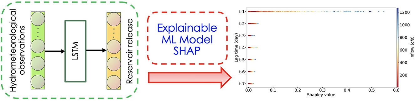
Figure 2. The framework of investigating the hydrometeorological influences on reservoir releases in this study. First, a LSTM model is trained for the reservoir release prediction and then the SHAP analysis is used to evaluate the variable importance and variable-wise temporal importance. Lastly, we assess the physical reliability of the SHAP explanation.

For each reservoir, we use 80% of its data record as a training set to construct and calibrate the LSTM model, and then use the rest of 20% of the data as a test set to evaluate the model prediction performance. The data record is split sequentially and uses a unit of years. For example, reservoir CRY has 30 years of data from 1982, then the first 24 years of data (i.e., 01/01/1982–12/31/2005) are in the training period and the subsequent 6 years of data (i.e., 01/01/2006–12/31/2011) are in the test period. The 80:20 ratio on training-test data split was generally taken in machine learning studies (Joseph, 2022), and it is also suitable for our problems here. In the results, we demonstrate that the 80% training data are able to learn the input-output relationship and the remaining 20% test data provide a good representative data set to evaluate the model prediction performance under different meteorological and reservoir management conditions.

LSTM models have several hyperparameters that need to be determined before they can be used for prediction, such as those parameters related to network architectures, learning rates, and the look-back window size t of the input sequence. The t value is particularly important (Zhang et al., 2019), which determines the lag length of input observations used to generate the model output, i.e., the t value represents the period over which the influence of hydrometeorological inputs is taken into account to calculate the reservoir release. We use 20% of the training data as the validation set for the hyperparameter tuning. In this process, we consider a set of possible values for each hyperparameter and evaluate the model prediction performance for all the hyperparameter combinations, and then select the set of hyperparameters giving the best performance on the validation set. After the tuning, we use the following hyperparameters for our LSTM model simulation. In terms of the model structure, we use one hidden layer with different numbers of nodes for different reservoirs. For example, 100 nodes for reservoir NAV with a long record of data, and 20 nodes for reservoir CAU with a relatively short period of data. For all the reservoirs, the Adam optimizer with the batch size of 20 and the learning rate of 0.001 are applied and the training ends at the epoch of 200. All the four input variables are scaled into the range of [0,1] to facilitate the training. Additionally, we use the previous 7 days of the hydrometeorological observations for reservoir release prediction (i.e., t = 7), which demonstrate the best prediction performance on the validation data among the range of t values between 1 and 15 (Fan et al., 2022b). Correspondingly, we investigate the hydrometeorological influence on the reservoir release in this 7-day period.

2.6. Model evaluation metrics

We employ six statistical metrics widely used in hydrological community (Gupta et al., 2009; Yang et al., 2021) to evaluate the LSTM model prediction performance, which includes the Correlation Coefficient (CORR), the Root Mean Squared Error (RMSE), the Nash-Sutcliffe Model Efficiency Coefficient (NSE), Kling-Gupta Efficiency (KGE), RMSE-observation standard deviation ratio (RSR), and Percent bias (PBIAS). They are defined as follows.

$\begin{array}{ll}CORR=\frac{{\displaystyle {\sum }_{k=1}^n}\left((S_k-\overline{S_k})(O_k-\overline{O_k})\right)}{\sqrt{{\displaystyle {\sum }_{k=1}^n}{\left(S_k-\overline{S_k}\right)}^2{\displaystyle {\sum }_{k=1}^n}{\left(O_k-\overline{O_k}\right)}^2}}& (12)\end{array}$

$\begin{array}{ll}NSE=1-\frac{{\displaystyle {\sum }_{k=1}^n}{\left(S_k-O_k\right)}^2}{{\displaystyle {\sum }_{k=1}^n}{\left(O_k-\overline{O_k}\right)}^2}& (13)\end{array}$

$\begin{array}{ll}KGE=1-\sqrt{{(1-CORR)}^2+{(1-{\sigma }_S/{\sigma }_O)}^2+{(1-{\mu }_S/{\mu }_O)}^2}& (14)\end{array}$

$\begin{array}{ll}RMSE=\sqrt{\frac{{\displaystyle {\sum }_{k=1}^n}{(S_k-O_k)}^2}{n}}& (15)\end{array}$

$\begin{array}{ll}RSR=\frac{\sqrt{{\displaystyle {\sum }_{k=1}^n}{\left(O_k-S_k\right)}^2}}{\sqrt{{\displaystyle {\sum }_{k=1}^n}{\left(O_k-\overline{O_k}\right)}^2}}& (16)\end{array}$

$\begin{array}{ll}PBIAS=\frac{{\displaystyle {\sum }_{k=1}^n}\left(O_k-S_k\right)\times 100}{{\displaystyle {\sum }_{k=1}^n}(O_k)}& (17)\end{array}$

Where S_k and O_k are the predicted and observed values, respectively, and $\overline{S_k}$ and $\overline{O_k}$ are their corresponding averages; σ_S and μ_S are the mean and standard deviation of the predicted values; σ_O and μ_O are the mean and standard deviation of the observed values; and n is the total number of observations.

The measurements of CORR, RMSE, and NSE are widely used statistical measures to quantify how the simulated reservoir release matches the observed release. CORR measures how the simulated time series data vary with the corresponding observations. RMSE quantifies the accumulated biases between the prediction and observation. As a combined statistic of both CORR and RMSE, NSE reflects both the temporal variation and bias between the prediction and observation. KGE can amend some shortcomings of the NSE measurments by decomposing NSE values into linear correlation, bias, and variability components. PBIAS quantifies the percentage of biases between the prediction and observation. Based on above definitions, the criteria of RMSE, RSR, and PBIAS with a value of zero, and the metric of CORR, NSE, and KGE having a value of 1 indicate the best prediction accuracy. According to previous studies (Moriasi et al., 2007; Yang et al., 2021), the model performance and the NSE/KGE scores have the following correspondence: NSE/KGE > 0.75: Very good prediction; 0.65 < NSE/KGE ≤ 0.75: Good prediction; 0.5 < NSE/KGE ≤ 0.65: Satisfactory prediction; 0.4 < NSE/KGE ≤ 0.5: Acceptable prediction; and NSE/KGE ≤ 0.4: Unsatisfactory prediction.

3. Results

In this section, we first present the reservoir release prediction results using LSTM networks based on four hydrometeorological inputs using their 7-day lag observations and evaluate the prediction performance using multiple statistics. Then, we use SHAP to identify the four hydrometeorological factors' contributions to the reservoir release prediction. Last, we verify the correctness of temporal importance determined from the SHAP method for the hydrological factors and investigate their long-term effects on the reservoir release prediction.

3.1. LSTM model prediction performance

In this section, we present the summary of six statistical measurements in the test period for 30 reservoirs, as illustrated in Table 2. The statistical values for all 30 reservoirs are summarized with the following range: 0.83 ≤ CORR ≤ 1.00, 0.69 ≤ NSE ≤ 0.99, 0.52 ≤ KGE ≤ 0.98, 0.21 ≤ RMSE ≤ 9.35, 0.10 ≤ RSR ≤ 0.56, and −34.15% ≤ PBIAS ≤ 22.98%. According to the NSE categorization defined in Section 2.6, 28 reservoirs are categorized as very good predictions and the other two reservoirs are categorized as good predictions, which indicates the LSTM model's capability to successfully capture the variations of daily reservoir releases. The other five metrics present a consistently good forecasting performance as the NSE. This remarkably good prediction performance on these diversely featured reservoirs demonstrates that LSTM models can effectively extract the long-term dependence information from hydrometeorological variables and successfully forecast the reservoir release.

TABLE 2

Table 2. The summary of LSTM model prediction performance on the reservoir release.

According to the study of Yang et al. (2021), the ML model prediction performance can be affected by many factors, including the reservoir elevation, the maximum capacity of the reservoir storage, and the primary function, etc. In the following, we analyze three different featured reservoirs, including the reservoir HYR with a low elevation, reservoir NAV with a large capacity of storage, and reservoir FGR with a hydropower functionality in more detail. We will demonstrate that even though these factors could conjunctively affect the human-controlled release decision, the LSTM model can capture the embedded information from historical observation data and effectively simulate the reservoir release and human's decision-making process.

Figure 3 illustrates the observed and LSTM-predicted daily release at the reservoir HYR in both training and test periods with NSE scores being 0.91 and 0.93, respectively. As observed, although the reservoir HYR has the lowest elevation which may increase the management complexity for the LSTM model to forecast the human's release decision, the predicted reservoir release closely matches the observations. Taking a detailed analysis of the release patterns, we can observe that reservoir HYR has a regular seasonal variation in the controlled reservoir release for most of years. This is because the reservoir refills in the Upper Colorado River region are mainly dominated by the seasonal runoff produced by melting snow and mountainous hydrology instead of the heavy precipitation from the atmospheric river events, where the water routing in upstream river basins can notably influence the release decisions of downstream reservoirs. Despite these challenges, the LSTM model can still capture the reservoir release variations even at certain years when there is an abnormally large reservoir release. Furthermore, the upstream operation and coordination between reservoirs are affected by different operation policies and interests, which can further increase the difficulty in forecasting the releases for reservoirs with lower elevations. Nevertheless, the high prediction performance demonstrates that the LSTM model can capture the high variation information brought from the upstream reservoir management.

FIGURE 3

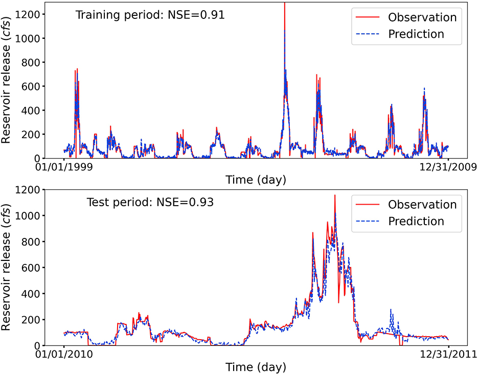
Figure 3. Observed and LSTM-predicted daily release at reservoir HYR. The LSTM model provides an accurate prediction with high NSE scores, although reservoir HYR has the lowest elevation, which is more susceptible to the influences from water routing in upstream river basins and possible releases from reservoirs with higher elevations.

Figure 4 depicts the observations and predictions of daily release at reservoir NAV with NSE scores being 0.94 and 0.83 for the training and test periods, respectively. Although the LSTM model misses some peak flows, it can accurately capture the release patterns and predict the timings of the peak reservoir releases, which is crucial for flood control and water resources management. Taking a detailed inspection, it can be observed that the fluctuations at low flow regimes are small, and when it releases water, a great volume of water is discharged within a short period of time. This is because when the reservoir (e.g., NAV) has a large storage capacity, it plays multiple functions roles such as agriculture irrigation, ecosystem productivity, and recreation, and thus is associated with more constraints and operation criteria. Therefore, the lack of flexibility in adjusting to the reservoir inflow variations may lead to more challenges for the LSTM model to capture human's release decisions.

FIGURE 4

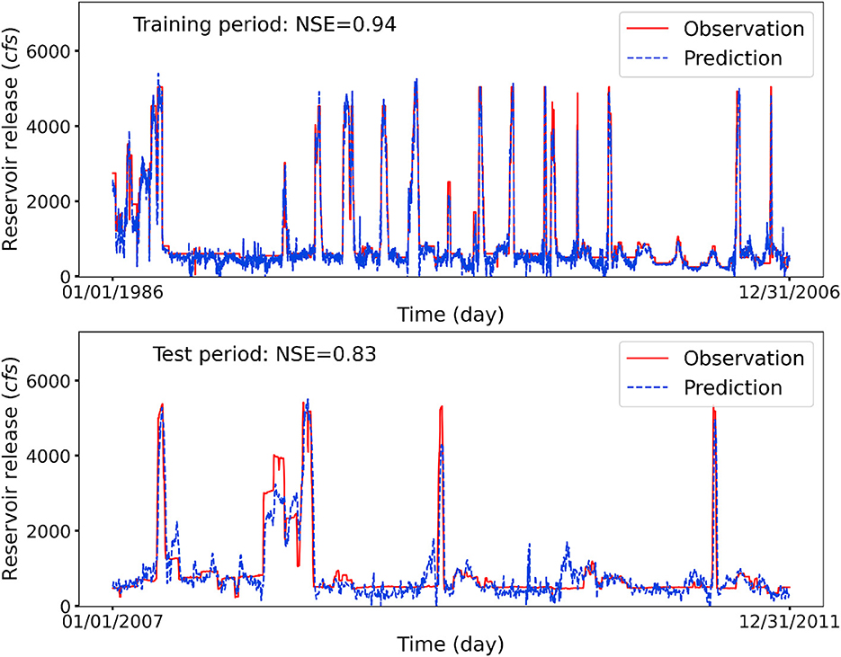
Figure 4. Observed and LSTM-predicted daily release at reservoir NAV. The LSTM model provides an accurate reservoir release forecasting despite the erratic release patterns caused by the large storage capacity.

As expected, the LSTM predicted daily release are in great agreement with the observations at reservoir FGR with NSE scores being 0.95 and 0.96 for the training and test periods, as illustrated in Figure 5. It is clearly observed that the reservoir FGR has many non-smooth variations in release patterns at low flow regimes. This is because the reservoir function such as the hydro-electric power generation, also plays a crucial role in the operation decision-making process. For reservoirs with the functionality of hydropower generation, when providing hydroelectric supplies to meet the energy demands during peak hours, the water is required to be diverted to the powerhouse first to enable the system to be flexibly turned on and off (Ding et al., 2021). Despite this irregular reservoir release because of the required reserves to effectively stabilize the power grid variations, the high agreement between the observation and predicted reservoir release demonstrates the LSTM model's capacity in accurately capturing human's release decisions.

FIGURE 5

Figure 5. Observed and LSTM-predicted daily release at reservoir FGR. The LSTM model accurately capture the release flow patterns, although reservoir FGR has irregular daily releases because of hydro-electric power generation.

We use multi-step lag observations of four hydrometeorological factors to accurately forecast the reservoir release in the 30 reservoirs of the Upper Colorado River Basin. To help operators comprehensively understand how LSTM makes reservoir release predictions from hydrometeorological variables, we use SHAP to investigate the contribution of each hydrometeorological factor to the amount of water to be released and the temporal importance of hydrological factors in the reservoir release forecasting. More importantly, we explore whether SHAP can provide reliable and physically plausible explanations for the hydrological processes being simulated by the LSTM model.

3.2. The importance of hydrometeorological factors identification

In this section, we compute the Shapley value for each input variable in the LSTM model at each time step using the test data and then average each hydrometeorological factor importance over 7 days. Next, we design experiments to examine the correctness of the contribution of each factor to the prediction determined by the SHAP analysis. Last, we use domain knowledge to assess the physical realism of the inferred hydrological processes.

Figure 6 presents the importance of four hydrometeorological factor contributions determined from the SHAP analysis. To ensure a fair comparison among different reservoirs, the importance scores of four hydrometeorological factors for each reservoir are normalized such that the sum of the importance scores of four features is one. As illustrated in Figure 6, all the reservoirs are categorized into two groups, where the reservoirs with a relatively small storage capacity are highlighted in yellow and the reservoirs with a relatively large storage capacity are highlighted in blue. It is clearly observed that the inflow is the dominant factor of reservoir release prediction for the small reservoirs and the storage will dominate the reservoir release forecasting for the large reservoirs. Overall, the top two contributors are storage and inflow and both the temperature and precipitation play a minor role in forecasting the reservoir daily release. This finding is consistent with the domain knowledge that the hydrological factors have more influence than the meteorological factors, since the climate forcing tends to have a hysteresis effect on the reservoir inflow.

FIGURE 6

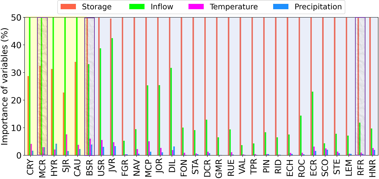
Figure 6. The importance of four hydrometeorological factors determined from the SHAP analysis. When the reservoir has a small storage capacity, the inflow is the dominant factor (highlighted in yellow). When the reservoir has a relatively large storage capacity, the storage is the dominant factor (highlighted in blue).

Next, we verify the feature contributions determined from the SHAP analysis. Specifically, we select three representative reservoirs to design experiments: when the inflow is the primary driver for the release forecasting, we design an additional experiment for reservoir MCR that only considers inflow; when both the inflow and storage are the main drivers for the release forecasting, we perform three additional experiments for reservoir BSR, where experiment I considers inflow only, experiment II considers storage only, and experiment III considers both inflow and storage; when the storage is the dominant factor for the release forecasting, we perform two additional experiments for reservoir RFR, where experiment I considers storage only and experiment II considers both inflow and storage. All experiments use 7-day lag observations as input variables.

Based on the SHAP analysis illustrated in Figure 6, the inflow is the dominant driver in affecting the release prediction for reservoir MCR. Therefore, we design an experiment to test whether only considering inflow can obtain a good forecasting of the reservoir's daily releases forecasting. As illustrated in Figure 7, the high NSE score of using only inflow as the input to forecast the reservoir release verifies the correctness of SHAP analysis. From the perspective of domain knowledge, small reservoirs are subjected to fewer constraints and operation criteria and thus easier to manage. In consequence, the reservoir operators can easily adjust the reservoir storage volumes in response to the variations in reservoir inflows. Therefore, the inflow plays a more important role for small reservoirs, and it affects reservoir release decisions. The feature importance determined from the SHAP method is consistent with the designed experiment results and domain knowledge.

FIGURE 7

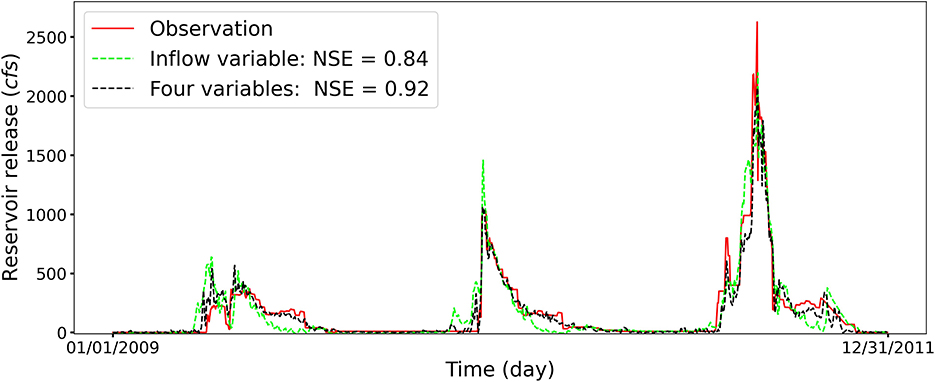
Figure 7. The comparison of prediction results for reservoir MCR between using four hydrometeorological variables and using only inflow variable as the LSTM input to forecast the daily reservoir release. The legend (Four variables) represents the experiment considering all four inputs of storage, inflow, temperature, and precipitation. The high NSE score of using only the inflow as input variable to predict the reservoir release verifies the SHAP result that the inflow is the dominant factor.

Although using only inflow to forecast the reservoir release can accurately capture the trend and peak timing, the LSTM model over- or under-estimate the reservoir release at different flow regimes. Specifically, due to the functionality of flood control, the reservoir MCR has a clear periodic water releasing pattern throughout the testing period. The reservoir operators will empty the reservoir storage for the required flood control during winter and make preparations for the spring snowmelt. Therefore, incorporating four hydrometeorological information can assist LSTM in capturing the reservoir inflow-release dynamics and improve the prediction accuracy, which is crucial for flood control and water management.

Based on the SHAP analysis, both the inflow and storage play important roles for reservoir BSR in affecting the reservoir release prediction. Therefore, we perform additional three experiments to assess the influence of inflow (experiment I), storage (experiment II), and both storage and inflow (experiment III) on the reservoir release forecasting. As illustrated in Figure 8, the NSE values are 0.66, 0.62, and 0.92 for experiments I, II, and III, respectively. It is clearly observed that using only inflow or storage to forecast the reservoir release leads to similar prediction performance, which tends to decrease the prediction accuracy. When both storage and inflow are used to forecast the reservoir release, the prediction accuracy improves significantly, which has a similar NSE score as the case including all four hydrometeorological factors. In the respective of hydrological knowledge, the functions of the reservoir storage and inflow are interconnected. The reservoir storage is a state variable, which collects and stores water from upstream river basins. The influence of the reservoir inflow on the reservoir release is affected by the amount of water kept in quantity and operation constraints in large reservoirs. Thus, both inflow and storage play important roles on the water release for reservoirs with relatively large storage capacities. The designed experiment results verify the analysis from the SHAP method, and the inferred physical process is consistent with the hydrological knowledge.

FIGURE 8

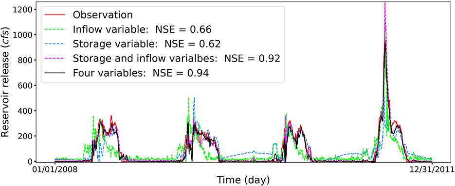
Figure 8. The predicted daily release of reservoir BSR for the four experiments using different hydrometeorological inputs. The legend (Four variables) represents the experiment considering all four inputs of storage, inflow, temperature, and precipitation. The feature importance learned from the SHAP method is consistent with the designed experiment result.

According to the SHAP analysis, the storage plays an important role in affecting the release prediction for the reservoir RFR. Therefore, we additionally design two experiments to evaluate whether the major prediction gains are from the storage feature for the reservoir RFR. Figure 9 illustrates the experiment predictions and observations for the reservoir RFR. As illustrated, using only storage to forecast the reservoir release leads to poor prediction performance, as well as overestimation at low flow regimes and underestimation at high flow regimes. However, using both storage and inflow to forecast the reservoir release can significantly improve the prediction performance, which achieves a high NSE score close to including all four hydrometeorological factors. With respect to the domain knowledge explanations, when the storage is the dominant factor and has a relatively small storage capacity (e.g., reservoir RFR), the storage buffer function of a reservoir is less significant, and the release is more susceptible to the variations of reservoir inflow. Under this circumstance, both the reservoir inflow and storage can affect the reservoir release. Therefore, the relatively low NSE score of using only storage as the input variable indicates that the feature importance selected from SHAP should be evaluated against the physical processes being modeled.

FIGURE 9

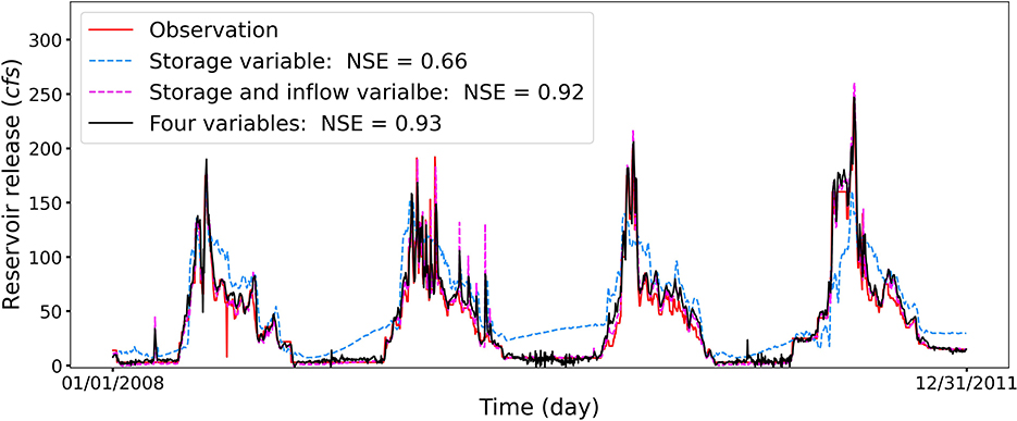
Figure 9. The predicted daily release of reservoir RFR for the three experiments using different hydrometeorological inputs. The legend (Four variables) represents the experiment considering all four inputs of storage, inflow, temperature, and precipitation. The relatively low NSE score of using only storage as the input variable demonstrates that using the feature importance selected from the SHAP analysis should refer to physical processes being modeled.

3.3. The temporal importance of hydrological factors identification

In this section, we investigate the temporal importance of hydrological factors in affecting reservoir release forecasting. Since the meteorological factors play minor roles in the reservoir release prediction, only the hydrological factors are used as the LSTM model inputs to predict the reservoir release. We first calculate Shapley values to determine the temporal importance of hydrological factors at each time step. The importance scores from the 3 to day 7 are combined because of decreased contributions to the release forecasting. Next, we design experiments to examine the temporal importance of hydrological factors determined by the SHAP analysis. Last, we evaluate the inferred physical process from the SHAP analysis against the domain hydrological knowledge.

Figure 10 presents the importance of reservoir storage and inflow determined from the SHAP analysis. To ensure a fair comparison among different reservoirs, the importance scores of each time step are normalized in each reservoir such that the sum of the importance scores of the two variables is one. The contributions of 7-day lag observations to the release prediction present different behaviors in different hydrological factors. For the reservoir storage factor, the first- and second-day lag observations are the dominant drivers in forecasting the reservoir release. Meanwhile, the rest 5 days' storage observations still have significant contributions to the release forecasting. For the reservoir inflow factor, the release prediction is mostly contributed by the inflow that occurred within the past 2 days. Compared to the storage factor, the rest 5 days' inflow observations play a minor role in forecasting the reservoir release.

FIGURE 10

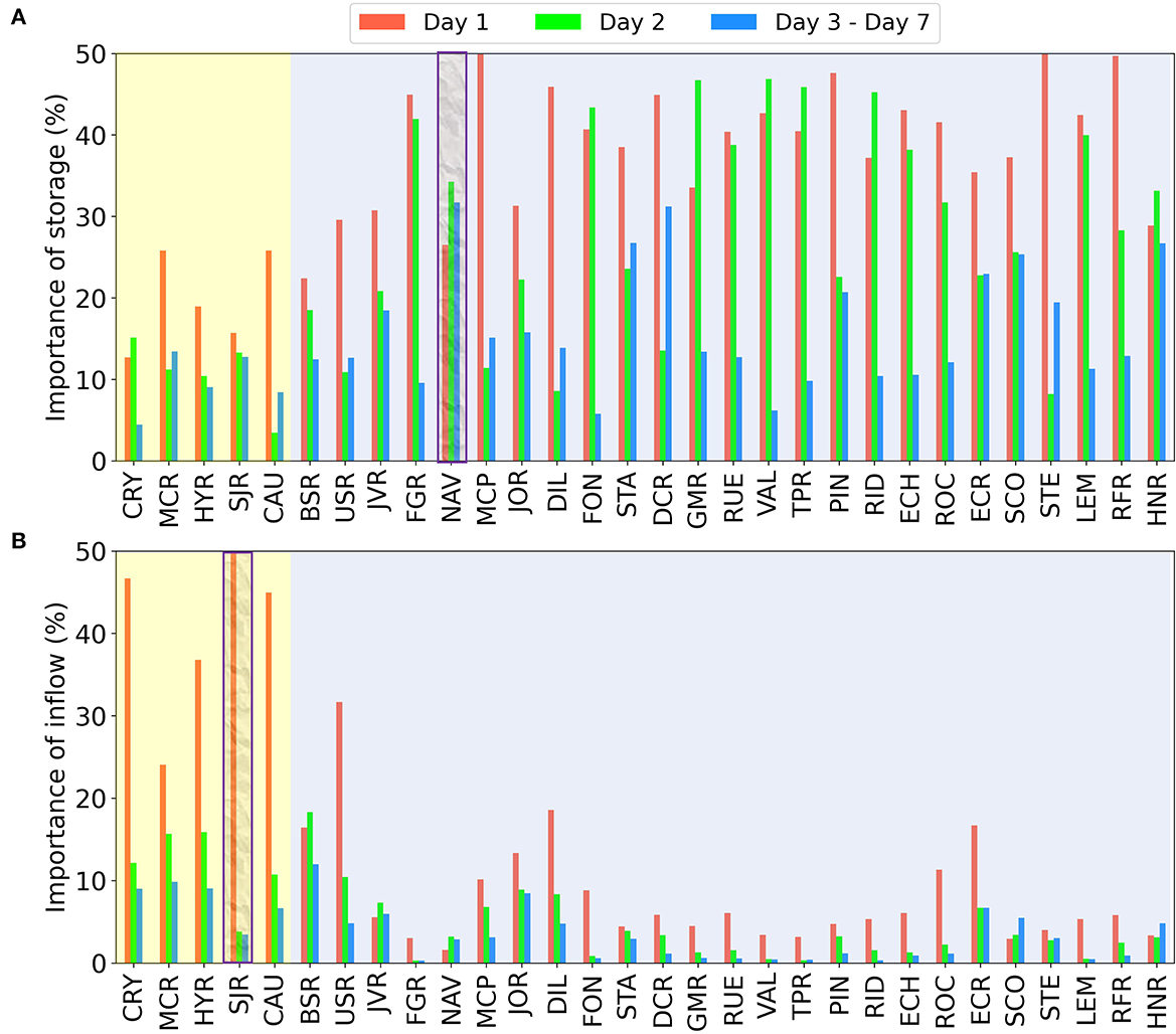
Figure 10. The temporal importance of reservoir (A) storage and (B) inflow determined from the SHAP analysis. The importance scores from day 3 to day 7 are combined. The SHAP analysis demonstrates that the first- and second-day lag observations have more influences on the release forecasting, which is consistent with the domain knowledge.

Next, we verify the temporal importance determined from the SHAP analysis. Specifically, we select two representative reservoirs to design experiments: for the storage factor, we examine its temporal importance in release forecasting for the reservoir NAV, since all 7 days have similar contributions to the release prediction; for the inflow factor, we evaluate its temporal importance in release forecasting for the reservoir SJR, because the first day is the dominant driver in the release forecasting. We compare the prediction performance from two experiments, where one using 7-day lag observations and the other using 2-day lag observations for both reservoir NAV and SJR. In both experiments, we only consider storage and inflow as the inputs.

According to the storage importance scores from the SHAP analysis, all 7 days' storage have significant contributions to the release forecasting for the reservoir NAV. Thus, we examine the Shapley values within the past 7 days for the reservoir NAV storage feature, as illustrated in Figure 11A. It can be observed that the storage observations that occurred within past 7 days all contribute significantly to the reservoir release forecasting. In general, the large storage values correspond to the large Shapley values, which indicates that the large storage has a more significant contribution to the release prediction. Figure 11B presents the predicted daily release of reservoir NAV for the two experiments using 7- and 2-day lag observations with NSE scores being 0.74 and 0.22, respectively. It can be clearly observed that with 2-day lag observations as inputs, the LSTM model fail to predict the reservoir release, which verifies the temporal importance analysis using the SHAP analysis. From the perspective of domain knowledge, since reservoir NAV has a large storage capacity, more lag observations will be evaluated to make the release decision. It is also noticeable that the Shapley values assigned to each day fluctuate across time steps for the reservoir NAV, which indicates that in the LSTM simulation, some days (e.g., days 1, 2, 4, and 5) have more important contributions to the release prediction when compared to others. However, this quantified importance for each time step deviates from the fact that storage of more recent time steps should have a higher impact on the reservoir release prediction. The results of this experiment show that inferred hydrological processes can be partially consistent with physical realism.

FIGURE 11

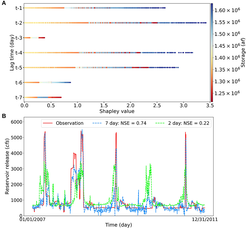
Figure 11. (A) The temporal Shapley values for the reservoir NAV storage factor. (B) The comparison of simulated reservoir releases between using 7 day lag and 2 day lag observations, where the legend (7 day) represents using previous 7 days of storage and inflow data to predict the reservoir release on the current day. The significantly improved accuracy of using 7-day lag observations is in consistent with the feature importance identified by the SHAP analysis.

As illustrated in Figure 10B, the inflow importance score for day 1 lag observation is significantly higher than the other days for the Reservoir SJR. We additionally designed an experiment to examine the temporal importance quantified by the SHAP analysis. Figure 12A illustrates the Shapley values for the lag 7-day inflow observations and presents that the past 1-day inflow observation has the most significant contribution to reservoir release forecasting. For reservoir SJR, a consistent pattern is observed that there are no large fluctuations in the importance of inflow within the past observations. The large Shapley values correspond to the large inflow values, which is also consistent with the hydrological knowledge that the small reservoirs (e.g., SJR) are more flexible to adjust to the variations of water release. Figure 12B presents the predicted reservoir release using 7- and 2-day lag observations along with the observed release with NSE scores being 0.97 for both two experiments. We can observe that using 2-day lag observations can also provide a good release prediction accuracy, which verifies the correctness of SHAP analysis. It is also noticeable that even though the metric score NSE is the same, using 7-day lag observations can help alleviate the over-estimations of reservoir releases at low-flow regimes. From the perspective of hydrological knowledge, the small reservoirs (e.g., SJR) are more sensitive to the inflow within past 2 days because the small storage leaves no room for the reservoir to store large amount of water and the inflow has direct influence on the release decision.

FIGURE 12

Figure 12. (A) The temporal Shapley values for the reservoir SJR inflow factor. (B) The comparison of simulated reservoir releases between using 7 day and 2 day lag observations, where the legend (7 day) represents using previous 7 days of stroage and inflow data to predict the reservoir release on the current day. For the reservoir SJR, the first 2 day information is the dominant driver in influencing the reservoir release. The little difference between two simulations confirms the correctness in using SHAP to identify the temporal feature importance.

4. Discussions

In this study, we first use LSTM to predict the reservoir daily release from the hydrometeorological drivers and then apply SHAP to the trained LSTM model to investigate the influence of these drivers on the prediction. The LSTM models have several hyperparameters that need to be determined before they can be used for prediction. The hyperparameter of look back window size (t value) is particularly important which determines the lag length of input observations used to predict the model output, i.e., the t value represents the period over which the influence of hydrometeorological inputs is taken into account to calculate the reservoir release. However, as a data-driven model, the t value in LSTM cannot be determined through physical constraints and mass balance equations. In this work, we use 20% of the training data as the validation set to tune the hyperparameters. Specifically, we consider a range of t from 1 to 15 and evaluate the prediction performance on the validation data for each t values. Results indicate that t = 7 days give the best prediction of the reservoir release. Take the reservoir CAU as an example, the following Figure 13 illustrates that the NSE value gradually increases as the increase of t at the beginning and achieves the highest value when the lag length t is 7 and then the performance drops again. We then use t = 7 for all the 30 reservoirs and find that it gives the best prediction performance on the validation data for most of the reservoirs. Therefore, in the numerical experiments of this study, we use previous 7 days of hydrometeorological observations for the reservoir release prediction.

FIGURE 13

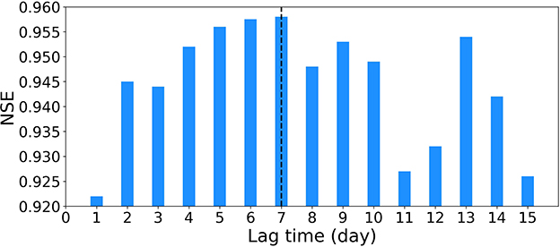
Figure 13. The NSE values in predicting reservoir release for the different lag length of hydrometeorological observations at reservoir CAU. The LSTM model yields the highest prediction accuracy when the lag length is 7.

A ML model is generally considered trustworthy if it can generate predictions in a way that is consistent with our knowledge of the system being modeled. SHAP is a model-agnostic explanation method. It can be generally applied to different ML models to explain the influence of model inputs on the outputs. Meanwhile, SHAP is a local method which does not consider variable interactions, which may result in some knowledge-inconsistent explanations. Moreover, SHAP could suffer from the unstable issue, i.e., multiple runs on the same data and the same model with the same parameter settings may result in different Shapley values. To address the possible instability of SHAP, for each reservoir, we perform 10 simulations of the SHAP analysis and use the mean value for explanation. We find that SHAP present stable results in this study where the 10 simulations have minor difference in SHAP values for all the 30 reservoirs. Take the reservoir SJR as an example, Figure 14 shows that for all the four hydrometeorological variables, the SHAP values at each time step are close to each other between the 10 simulations. For most of the 30 reservoirs, SHAP gives physics-consistent explanations on the variable importance and variable-wise temporal importance. But, in a few reservoirs it is difficult to interpret SHAP explanation on the temporal importance for a certain drivers from a hydrological point of view. For example, lag hydrological observations that occurred in the recent past generally have more impact on the release prediction. However, SHAP shows a slightly different pattern in this lag time influence of the storage variable for reservoir NAV. This is probably caused by the SHAP's ignorance of the variable interactions when it calculates attribution scores. In summary, SHAP is a useful tool for black-box ML model explanations, but the inferred physical processes should be cautiously evaluated against domain-specific hydrological knowledge to ensure the high prediction accuracy is associated with reasonable explanations.

FIGURE 14

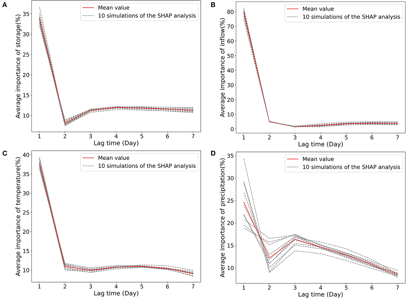
Figure 14. We perform 10 simulations of SHAP analysis and use the mean value for explanation. For all the four drivers, i.e., (A) inflow, (B) storage, (C) temperature, and (D) precipitation, their SHAP values are similar between the simulations, giving stable explanation, taking the reservoir SJR as an example here.

In the future, we will improve SHAP analysis to address its physics-inconsistent issues. Furthermore, we will apply our recently developed uncertainty quantification (UQ) method (Liu et al., 2022; Lu et al., 2022a; Zhang P. et al., 2022) to evaluate the prediction uncertainty of reservoir release to address the influence of the data noise and to ensure a credible prediction under the climate change. Additionally, we will apply our proposed interpretable ML methods with UQ for the diverse reservoirs across the contiguous Unites States (CONUS) to improve the predictive understanding of the reservoir release and support decision making of the reservoir operators.

5. Conclusions

In this work, we use the LSTM network to predict reservoir release from its hydrometeorological drivers including inflow, storage, precipitation and temperature, and apply the SHAP analysis to explain the variable importance and the variable-wise temporal importance of these drivers on the release. In the application to 30 diverse reservoirs in the Upper Colorado River Basin, we demonstrate that the LSTM models can reasonably learn the relationship between the hydrometeorological drivers and the reservoir release from their observations and make an accurate prediction under different meteorological and reservoir conditions. Additionally, SHAP identifies that storage and inflow are the two most influential drivers which have a relatively long-term impact on the release and this impact gradually decreases as the lag time increases. This interpretation of SHAP analysis is consistent with our physical knowledge. However, in a few reservoirs, SHAP does not show a clear influence decay along the increase of the lag time, which is difficult to explain and probably caused by the SHAP's ignorance of the variable interactions. To summarize, SHAP is a good method to interpret learning and prediction of the black-box machine learning models. In this study, the SHAP analysis enhances our understanding of the LSTM simulation, improves the trustworthiness of the model prediction, and assists the reservoir operators in making climate-resilient decisions. Nevertheless, due to the incapability of SHAP in calculating the variable interactions, its results should be cautiously interpreted in practice. In the future, we will improve SHAP analysis and apply it to other machine learning tasks for trustworthy and reliable scientific predictions.

Data availability statement

The original contributions presented in the study are included in the article/supplementary material, further inquiries can be directed to the corresponding author.

Author contributions

MF: conceptualization, methodology, software, result interpretation, and writing—original draft. LZ: data processing, result interpretation, writing—review, and editing. SL: software, result interpretation, writing—review, and editing. TY: result interpretation, writing—review, and editing. DL: conceptualization, methodology, software, result interpretation, writing—review, and editing. All authors contributed to the article and approved the submitted version.

Funding

The major funding support for this work is provided by the waterpower project funded by the U.S. Department of Energy (DOE), Water Power Technologies Office. Additional support was from the Artificial Intelligence Initiative as part of the Laboratory Directed Research and Development Program of Oak Ridge National Laboratory, managed by UT-Battelle, LLC, for the US DOE under contract DE-AC05-00OR22725. This research was also sponsored by the Data-Driven Decision Control for Complex Systems (DnC2S) project funded by the U.S. DOE, Office of Advanced Scientific Computing Research. The work was also partially supported by the National Science Foundation under Grant No. OIA-1946093 and its subaward No. EPSCoR-2020-3, and the Oklahoma EPSCoR Research Seed Grand supported by NSF. This work was also partially supported by U.S. Department of Defense, Army Corps of Engineers (DOD-COR) Engineering With Nature (EWN) Program (Award No. W912HZ-21-2-0038).

Conflict of interest

The authors declare that the research was conducted in the absence of any commercial or financial relationships that could be construed as a potential conflict of interest.

Publisher's note

All claims expressed in this article are solely those of the authors and do not necessarily represent those of their affiliated organizations, or those of the publisher, the editors and the reviewers. Any product that may be evaluated in this article, or claim that may be made by its manufacturer, is not guaranteed or endorsed by the publisher.

References

Beven, K. (2020). Deep learning, hydrological processes and the uniqueness of place. Hydrol. Process. 34, 3608–3613. doi: 10.1002/hyp.13805

CrossRef Full Text | Google Scholar

Bozorg-Haddad, O., Aboutalebi, M., Ashofteh, P.-S., and Loáiciga, H. A. (2018). Real-time reservoir operation using data mining techniques. Environ. Monit. Assess. 190, 1–22. doi: 10.1007/s10661-018-6970-2

PubMed Abstract | CrossRef Full Text | Google Scholar

Chang, F.-J., Wang, Y.-C., and Tsai, W.-P. (2016). Modelling intelligent water resources allocation for multi-users. Water Resour. Manag. 30, 1395–1413. doi: 10.1007/s11269-016-1229-6

CrossRef Full Text | Google Scholar

Daly, C., and Bryant, K. (2013). The Prism Climate and Weather System–An Introduction. Corvallis, OR: PRISM Climate Group 2.

Google Scholar

Ding, Z., Wen, X., Tan, Q., Yang, T., Fang, G., Lei, X., et al. (2021). A forecast-driven decision-making model for long-term operation of a hydro-wind-photovoltaic hybrid system. Appl. Energy 291, 116820. doi: 10.1016/j.apenergy.2021.116820

CrossRef Full Text | Google Scholar

Duan, W., He, B., Nover, D., Yang, G., Chen, W., Meng, H., et al. (2016). Water quality assessment and pollution source identification of the eastern poyang lake basin using multivariate statistical methods. Sustainability 8, 133. doi: 10.3390/su8020133

CrossRef Full Text | Google Scholar

Duan, W., He, B., Takara, K., Luo, P., Nover, D., and Hu, M. (2015). Modeling suspended sediment sources and transport in the ishikari river basin, japan, using sparrow. Hydrol. Earth Syst. Sci. 19, 1293–1306. doi: 10.5194/hess-19-1293-2015

CrossRef Full Text | Google Scholar

Duan, W., Takara, K., He, B., Luo, P., Nover, D., and Yamashiki, Y. (2013). Spatial and temporal trends in estimates of nutrient and suspended sediment loads in the ishikari river, Japan, 1985 to 2010. Sci. Total Environ. 461, 499–508. doi: 10.1016/j.scitotenv.2013.05.022

PubMed Abstract | CrossRef Full Text | Google Scholar

Ehsani, N., Vörösmarty, C. J., Fekete, B. M., and Stakhiv, E. Z. (2017). Reservoir operations under climate change: Storage capacity options to mitigate risk. J. Hydrol. 555, 435–446. doi: 10.1016/j.jhydrol.2017.09.008

CrossRef Full Text | Google Scholar

Fan, M., Lu, D., Rastogi, D., and Pierce, E. M. (2022a). A spatiotemporal-aware weighting scheme for improving climate model ensemble predictions. J. Mach. Learn. Model. Comput. 3, 29–55. doi: 10.1615/JMachLearnModelComput.2022046715

CrossRef Full Text | Google Scholar

Fan, M., Zhang, L., Liu, S., Yang, T., and Lu, D. (2022b). Identifying Hydrometeorological Factors Influencing Reservoir Releases Using Machine Learning Methods. ICDMW 2022.

Google Scholar

Fryer, D., Strümke, I., and Nguyen, H. (2021). Shapley values for feature selection: the good, the bad, and the axioms. IEEE Access 9, 144352–144360. doi: 10.1109/ACCESS.2021.3119110

CrossRef Full Text | Google Scholar

García-Feal, O., González-Cao, J., Fernández-Nóvoa, D., Astray Dopazo, G., and Gómez-Gesteira, M. (2022). “Comparison of machine learning techniques for reservoir outflow forecasting,” in Natural Hazards and Earth System Sciences, 22, pp. 3859–3874. Available online at: https://nhess.copernicus.org/articles/22/3859/2022/

Google Scholar

Gupta, H. V., Kling, H., Yilmaz, K. K., and Martinez, G. F. (2009). Decomposition of the mean squared error and nse performance criteria: Implications for improving hydrological modelling. J. Hydrol. 377, 80–91. doi: 10.1016/j.jhydrol.2009.08.003

CrossRef Full Text | Google Scholar

Jiang, S., Zheng, Y., Wang, C., and Babovic, V. (2022). Uncovering flooding mechanisms across the contiguous united states through interpretive deep learning on representative catchments. Water Resour. Res. 58, e2021WR030185. doi: 10.1029/2021WR030185

CrossRef Full Text | Google Scholar

Joseph, V. R. (2022). Optimal ratio for data splitting. Stat. Anal. Data Min. 15, 531–538. doi: 10.1002/sam.11583

CrossRef Full Text | Google Scholar

Lees, T., Reece, S., Kratzert, F., Klotz, D., Gauch, M., De Bruijn, J., et al. (2022). Hydrological concept formation inside long short-term memory (LSTM) networks. Hydrol. Earth Syst. Sci. 26, 3079–3101. doi: 10.5194/hess-26-3079-2022

CrossRef Full Text | Google Scholar

Lin, Y., Wang, D., Wang, G., Qiu, J., Long, K., Du, Y., et al. (2021). A hybrid deep learning algorithm and its application to streamflow prediction. J. Hydrol. 601, 126636. doi: 10.1016/j.jhydrol.2021.126636

CrossRef Full Text | Google Scholar

Liu, S., Zhang, P., Lu, D., and Zhang, G. (2022). “PI3NN: out-of-distribution-aware prediction intervals from three neural networks,” in International Conference on Learning Representations. Available online at: https://arxiv.org/abs/2108.02327

Google Scholar

Liu, X., Chen, L., Zhu, Y., Singh, V. P., Qu, G., and Guo, X. (2017). Multi-objective reservoir operation during flood season considering spillway optimization. J. Hydrol. 552, 554–563. doi: 10.1016/j.jhydrol.2017.06.044

CrossRef Full Text | Google Scholar

Liu, Y., Qin, H., Zhang, Z., Yao, L., Wang, Y., Li, J., et al. (2019). Deriving reservoir operation rule based on bayesian deep learning method considering multiple uncertainties. J. Hydrol. 579, 124207. doi: 10.1016/j.jhydrol.2019.124207

CrossRef Full Text | Google Scholar

Lu, D., Konapala, G., Painter, S. L., Kao, S.-C., and Gangrade, S. (2021). Streamflow simulation in data-scarce basins using bayesian and physics-informed machine learning models. J. Hydrometeorol. 22, 1421–1438. doi: 10.1175/JHM-D-20-0082.1

CrossRef Full Text | Google Scholar

Lu, D., Liu, S., Painter, S. L., Griffiths, N. A., and Pierce, E. M. (2022a). “Uncertainty quantification of machine learning models to improve streamflow prediction under changing climate and environmental conditions,” in Earth and Space Science Open Archive, 26. Available online at: https://essopenarchive.org/users/533787/articles/598310-uncertainty-quantification-of-machine-learning-models-to-improve-streamflow-prediction-under-changing-climate-and-environmental-conditions?commit=7c4f59173fbca595e066c3951538b35e70d2b89e

Google Scholar

Lu, D., Ricciuto, D. M., and Liu, S. (2022b). An interpretable machine learning model for advancing terrestrial ecosystem predictions. Technical report, Oak Ridge National Lab.(ORNL), Oak Ridge, TN.

Google Scholar

Lundberg, S. M., Erion, G., Chen, H., DeGrave, A., Prutkin, J. M., Nair, B., et al. (2020). From local explanations to global understanding with explainable ai for trees. Nat. Mach. Intell. 2, 56–67. doi: 10.1038/s42256-019-0138-9

PubMed Abstract | CrossRef Full Text | Google Scholar

Lundberg, S. M., and Lee, S.-I. (2017). “A unified approach to interpreting model predictions,” in Advances in Neural Information Processing Systems, Vol. 30. Available online at: https://dl.acm.org/doi/10.5555/3295222.3295230

Google Scholar

Molnar, C. (2020). Interpretable Machine Learning. Available online at: Lulu.com.

Google Scholar

Moriasi, D. N., Arnold, J. G., Van Liew, M. W., Bingner, R. L., Harmel, R. D., and Veith, T. L. (2007). Model evaluation guidelines for systematic quantification of accuracy in watershed simulations. Trans. ASABE 50, 885–900. doi: 10.13031/2013.23153

CrossRef Full Text | Google Scholar

Murdoch, W. J., Singh, C., Kumbier, K., Abbasi-Asl, R., and Yu, B. (2019). Definitions, methods, and applications in interpretable machine learning. Proc. Natl. Acad. Sci. U.S.A. 116, 22071–22080. doi: 10.1073/pnas.1900654116

PubMed Abstract | CrossRef Full Text | Google Scholar

Niu, W.-J., Feng, Z.-K., Feng, B.-F., Min, Y.-W., Cheng, C.-T., and Zhou, J.-Z. (2019). Comparison of multiple linear regression, artificial neural network, extreme learning machine, and support vector machine in deriving operation rule of hydropower reservoir. Water 11, 88. doi: 10.3390/w11010088

CrossRef Full Text | Google Scholar

Rahnamay Naeini, M., Yang, T., Tavakoly, A., Analui, B., AghaKouchak, A., Hsu, K.-,l., et al. (2020). A model tree generator (mtg) framework for simulating hydrologic systems: application to reservoir routing. Water 12, 2373. doi: 10.3390/w12092373

CrossRef Full Text | Google Scholar

Reichstein, M., Camps-Valls, G., Stevens, B., Jung, M., Denzler, J., Carvalhais, N., et al. (2019). Deep learning and process understanding for data-driven earth system science. Nature 566, 195–204. doi: 10.1038/s41586-019-0912-1

PubMed Abstract | CrossRef Full Text | Google Scholar

Shen, C. (2018). A transdisciplinary review of deep learning research and its relevance for water resources scientists. Water Resour. Res. 54, 8558–8593. doi: 10.1029/2018WR022643

CrossRef Full Text | Google Scholar

Slack, D., Hilgard, A., Singh, S., and Lakkaraju, H. (2021). Reliable post-hoc explanations: modeling uncertainty in explainability. Adv. Neural Inf. Process. Syst. 34, 9391–9404. Available online at: https://arxiv.org/abs/2008.05030

Google Scholar

Slack, D., Hilgard, S., Jia, E., Singh, S., and Lakkaraju, H. (2020). “Fooling lime and shap: Adversarial attacks on post-hoc explanation methods,” in Proceedings of the AAAI/ACM Conference on AI, Ethics, and Society, 180–186. doi: 10.1145/3375627.3375830

CrossRef Full Text | Google Scholar

Song, X., Hao, H., Liu, W., Wang, Q., An, L., Yeh, T.-C. J., et al. (2022). Spatial-temporal behavior of precipitation driven karst spring discharge in a mountain terrain. J. Hydrol. 612, 128116. doi: 10.1016/j.jhydrol.2022.128116

CrossRef Full Text | Google Scholar

Sundararajan, M., and Najmi, A. (2020). “The many shapley values for model explanation,” in International Conference on Machine Learning (PMLR), 9269–9278. Available online at: https://proceedings.mlr.press/v119/sundararajan20b.html

Google Scholar

Uysal, G., Alvarado-Montero, R., Schwanenberg, D., and Şensoy, A. (2018). Real-time flood control by tree-based model predictive control including forecast uncertainty: a case study reservoir in turkey. Water 10, 340. doi: 10.3390/w10030340

CrossRef Full Text | Google Scholar

Yang, T., Asanjan, A. A., Welles, E., Gao, X., Sorooshian, S., and Liu, X. (2017). Developing reservoir monthly inflow forecasts using artificial intelligence and climate phenomenon information. Water Resour. Res. 53, 2786–2812. doi: 10.1002/2017WR020482

CrossRef Full Text | Google Scholar

Yang, T., Gao, X., Sorooshian, S., and Li, X. (2016). Simulating california reservoir operation using the classification and regression-tree algorithm combined with a shuffled cross-validation scheme. Water Resour. Res. 52, 1626–1651. doi: 10.1002/2015WR017394

CrossRef Full Text | Google Scholar

Yang, T., Liu, X., Wang, L., Bai, P., and Li, J. (2020). Simulating hydropower discharge using multiple decision tree methods and a dynamical model merging technique. J. Water Resour. Plann. Manag. 146, 04019072. doi: 10.1061/(ASCE)WR.1943-5452.0001146

PubMed Abstract | CrossRef Full Text | Google Scholar

Yang, T., Zhang, L., Kim, T., Hong, Y., Zhang, D., and Peng, Q. (2021). A large-scale comparison of artificial intelligence and data mining (ai&dm) techniques in simulating reservoir releases over the upper colorado region. J. Hydrol. 602, 126723. doi: 10.1016/j.jhydrol.2021.126723

CrossRef Full Text

Yang, Y., and Chui, T. F. M. (2021). Modeling and interpreting hydrological responses of sustainable urban drainage systems with explainable machine learning methods. Hydrol. Earth Syst. Sci. 25, 5839–5858. doi: 10.5194/hess-25-5839-2021

CrossRef Full Text | Google Scholar

Yu, Y., Si, X., Hu, C., and Zhang, J. (2019). A review of recurrent neural networks: LSTM cells and network architectures. Neural Comput. 31, 1235–1270. doi: 10.1162/neco_a_01199

PubMed Abstract | CrossRef Full Text | Google Scholar

Zhang, D., Lin, J., Peng, Q., Wang, D., Yang, T., Sorooshian, S., et al. (2018). Modeling and simulating of reservoir operation using the artificial neural network, support vector regression, deep learning algorithm. J. Hydrol. 565, 720–736. doi: 10.1016/j.jhydrol.2018.08.050

CrossRef Full Text | Google Scholar

Zhang, D., Peng, Q., Lin, J., Wang, D., Liu, X., and Zhuang, J. (2019). Simulating reservoir operation using a recurrent neural network algorithm. Water 11, 865. doi: 10.3390/w11040865

CrossRef Full Text | Google Scholar

Zhang, D., Wang, D., Peng, Q., Lin, J., Jin, T., Yang, T., et al. (2022). Prediction of the outflow temperature of large-scale hydropower using theory-guided machine learning surrogate models of a high-fidelity hydrodynamics model. J. Hydrol. 606, 127427. doi: 10.1016/j.jhydrol.2022.127427

CrossRef Full Text | Google Scholar

Zhang, P., Liu, S., Lu, D., Sankaran, R., and Zhang, G. (2022). An out-of-distribution-aware autoencoder model for reduced chemical kinetics. Discrete Contin. Dyn. Syst. 15, 913–930. doi: 10.3934/dcdss.2021138

PubMed Abstract | CrossRef Full Text | Google Scholar

Zolfaghari, M., and Golabi, M. R. (2021). Modeling and predicting the electricity production in hydropower using conjunction of wavelet transform, long short-term memory and random forest models. Renewable Energy 170, 1367–1381. doi: 10.1016/j.renene.2021.02.017

CrossRef Full Text | Google Scholar