 Adam M. Collins1*†
 Peter Rivera-Casillas2
 Sourav Dutta3
 Orie M. Cecil4
 Andrew C. Trautz5Matthew W. Farthing4
- 1Coastal and Hydraulics Laboratory, U.S. Army Engineer Research and Development Center, Duck, NC, United States
- 2Information Technology Laboratory, U.S. Army Engineer Research and Development Center, Vicksburg, MS, United States
- 3Oden Institute for Computational Engineering and Sciences, The University of Texas at Austin, Austin, TX, United States
- 4Coastal and Hydraulics Laboratory, U.S. Army Engineer Research and Development Center, Vicksburg, MS, United States
- 5Geotechnical and Structures Laboratory, U.S. Army Engineer Research and Development Center, Vicksburg, MS, United States
The goal of this study is to leverage emerging machine learning (ML) techniques to develop a framework for the global reconstruction of system variables from potentially scarce and noisy observations and to explore the epistemic uncertainty of these models. This work demonstrates the utility of exploiting the stochasticity of dropout and batch normalization schemes to infer uncertainty estimates of super-resolved field reconstruction from sparse sensor measurements. A Voronoi tessellation strategy is used to obtain a structured-grid representation from sensor observations, thus enabling the use of fully convolutional neural networks (FCNN) for global field estimation. An ensemble-based approach is developed using Monte-Carlo batch normalization (MCBN) and Monte-Carlo dropout (MCD) methods in order to perform approximate Bayesian inference over the neural network parameters, which facilitates the estimation of the epistemic uncertainty of predicted field values. We demonstrate these capabilities through numerical experiments that include sea-surface temperature, soil moisture, and incompressible near-surface flows over a wide range of parameterized flow configurations.
1. Introduction
High-resolution reconstruction (super-resolution) of sparsely sensed flow fields is important for, but not limited to, hydraulic and hydrological applications. The most successful approaches for super-resolution modeling of dynamical physical systems using sparse measurements have primarily involved deep learning approaches, specifically variations on convolutional neural networks (CNNs) and generative adversarial networks (GANs) (Deng et al., 2019; Fukami et al., 2019, 2021; Liu et al., 2020; Wang and Ročková, 2020; Bode et al., 2021; Gao et al., 2021; Wang L. et al., 2021; Zayats et al., 2022; Zhou et al., 2022). These methods include both residual loss functions, which minimize the disparity between predicted and target values, and physics-informed (PI) loss functions, where physical laws are enforced to supplement the learning process with relevant information about higher-resolution features, thus effectively solving a sub-grid modeling problem. However, deep learning methods tend to suffer from a so-called “black box” issue, which makes it difficult to interpret results from trained models using the same techniques that are traditionally applied to analytical models. Hence, reliable estimates of where a given model can fail are important for most applications. While there is burgeoning research on the explainability of neural networks (Goldstein et al., 2015; Carvalho et al., 2019; Nori et al., 2019; Apley and Zhu, 2020) (and many others), these results are often for simpler models and cases that are not in the scope of technological readiness for dynamical physical systems. Additionally, many situations exist where the interpretability of a model may be less critical than a measure of prediction uncertainty, especially for regimes that do not often have a solid mathematical theory. Because of this, and to sidestep the issue of infancy of explainability in deep learning, uncertainty quantification of machine learning models has become popular as a corollary with regards to estimating areas with a potential for high errors (Pearce et al., 2018; Kar and Biswas, 2019; Cortinhal et al., 2020; Wang and Ročková, 2020; Abdar et al., 2021). To this end, we present an exploration of low-shot single-image uncertainty estimation for the super-resolution of dynamical physical systems with sparse sensors.
1.1. Machine learning for super-resolution
The rapid development in the field of modern machine learning (ML) methods has created new and transformative approaches to not only approximate and accelerate existing numerical models but also solve a wide array of challenging problems in various areas of computational science. By leveraging the capabilities to incorporate multi-fidelity data streams from diverse sources, seamlessly explore massive design spaces, and identify complex, multivariate correlations, a variety of data-driven, ML-based methods have been proposed for image processing (Krizhevsky et al., 2017; Wang et al., 2020), inverse problems (Collins et al., 2020; Qian et al., 2020; Patel et al., 2022) reduced order modeling (Dutta et al., 2021a,b, 2022), solution of systems of partial differential equations (Chen et al., 2018; Raissi et al., 2019; Kadeethum et al., 2021), and turbulence modeling (Duraisamy et al., 2019; Beck and Kurz, 2021) to name a few. In particular, ML has also proven adept at super-resolution tasks (Wang et al., 2020) for dynamical physical systems by utilizing variations of CNNs (Liu et al., 2020), fully convolutional neural networks (FCNNs) (Fukami et al., 2019), and GANs (Kim et al., 2021; Güemes et al., 2022). Fukami et al. (2019, 2021) developed a field reconstruction approach for sparse sensors based on Voronoi tessellation and FCNNs, which was first applied to fluid flow and then to large-scale geospatial problems. Their introduction of a Downsampled Skip-Connection Multi-Scale (DSC/MS) model (Fukami et al., 2019), which features skip connections between the downsampling and upsampling blocks of the FCNN, showed superior results than CNNs in reconstructing turbulent flows. Supervised, self-supervised, and unsupervised methods have also been developed using CNNs (Maulik et al., 2019; Gao et al., 2021; Zayats et al., 2022) and GANs (Bode et al., 2019, 2021; Li and McComb, 2022) augmented with physics-informed (PI) loss functions.
A primary goal of developing a super-resolution methodology that can be applied to fluid flow scenarios is to create a framework that can ingest sparsely sensed measurements from multi-fidelity sources like wind tunnel experiments or low-cost, distributed field observations and produce high-resolution field reconstructions that are easily amenable for further analysis. Unfortunately, data collected from experimental and field measurement sources, like the ones mentioned above, can often be scarce. However, fluid flow problems are usually governed by known physical laws and conservation principles like the incompressible Navier-Stokes equations and the depth-averaged shallow water equations. Loss functions augmented with PI constraints defined by these governing equations can help alleviate the need for large amounts of training data in purely supervised learning, the downside is that PI networks are often resource intensive to train. Additionally, they may require measurements or estimates of the necessary fields to solve the physics constraints that are applicable to the scenario at hand (Karniadakis et al., 2021). In practice, due to sensor cost and limitations on the resolution of obtained measurements, data collection is often necessarily constrained, resulting in sparse spatiotemporal measurements with emphasis given to only a few relevant variables. For instance, one of the numerical experiments adopted in this study involves mean fluid flow over multiple surface geometries simulated by time-averaging of Direct Numerical Simulation (DNS)/Large Eddy Simulation (LES) results (McConkey et al., 2021). In order to effectively constrain the learning process with relevant governing equations such as the incompressible Navier-Stokes equations or the Reynolds-averaged Navier-Stokes equations and avoid well-known gradient flow pathologies (Wang S. et al., 2021), the neural network model would need well-resolved simulation or experimental data for each component of the system, namely velocity, pressure, and density. The collection of such data, simulation-based or experimental, may be limited by computational or observational constraints as discussed before. Alternatively, if only partial data for a particular component of the system, such as velocity is available, then the network would have to learn multiple unseen fields in order to train with the full system of governing equations as PI constraints; this would add even more computational complexity to the training and convergence of the model. Because of these drawbacks of both supervised and self/unsupervised approaches that use either purely residual or the full set of relevant physics-informed loss constraints, the methods explored here combine supervised and self/unsupervised techniques to mitigate the issues of both supervised training (large datasets) and self/unsupervised training (resource/variable intensive), which could prove useful in various applied scenarios.
1.2. Uncertainty estimation for machine learning in super-resolution
Some of the most common methods for uncertainty estimation in machine learning have focused on Bayesian approaches (or approximations thereof) (Osband, 2016; Wang and Ročková, 2020; Abdar et al., 2021). One of the most straightforward methods to approximate Bayesian inference is to use Bayesian Neural Networks (BNNs) (Blundell et al., 2015), which learn both a mean and a deviation instead of a scalar value for the network weights. This allows for an ensemble of predictions by repeatedly predicting on the same input image and looking at the variance of predictions created by the fluctuating network parameters. These provide an advantage over deterministic networks by allowing for a probabilistic prediction of the distribution of the predicted output; it is the variability in these distributions that are often interpreted as model uncertainty. However, this suffers from the same pitfall as typical Bayesian calculations (Minka, 2001) in that they are extremely resource-intensive to implement and train.
Another method for estimating uncertainty with neural networks involves the creation of an ensemble of trained models. There are various methods (Pearce et al., 2018; Malinin et al., 2019; Abdar et al., 2021) (both Bayesian and non-Bayesian) to combine with model ensembling to estimate confidence. However, while these methods improve on BNNs by not requiring as much memory to train the models (if trained sequentially), the amount of time it takes to create an analysis framework scales linearly with the number of models desired in the ensemble.
Due to the resource-intensive drawbacks of BNNs and ensembles of models, there has also been intense research on methods to estimate the epistemic uncertainty of a single trained model. One of the popular methods called Monte Carlo dropout (MCD) (Gal and Ghahramani, 2016; Gal et al., 2017; Wang and Ročková, 2020; Abdar et al., 2021) utilizes dropout during the testing step to generate an ensemble of model predictions. In Gal and Ghahramani (2016), Gal et al. showed that such an ensemble of predictions can be interpreted in an approximate Bayesian sense to be the Monte Carlo samples of the predictive distribution. Another technique for creating ensembles from a single model includes Monte Carlo batch normalization (MCBN), which has also been shown to approximate Bayesian inference techniques (Teye et al., 2018; Atanov et al., 2019; Kar and Biswas, 2019). Data augmentation is a technique typically employed during the training process to induce robustness in the model for unseen inputs. It has recently been shown to have the ability to approximate results obtained using Gaussian processes during test-time (Jiang et al., 2022). This work develops a framework for super-resolution that utilizes a Voronoi tessellation-based method to generate coarse, gridded training samples from sparse observations, and adopts the MC dropout and MC batch normalization techniques to generate an ensemble of super-resolved predictions such that the ensemble variance provides an estimate of the model uncertainty.
2. Approach
2.1. Supervised training
For this investigation, two well-known training strategies were explored that have seen a lot of success for single-image super-resolution tasks, namely supervised learning using FCNN architectures and adversarial training. The FCNN we used for this model was based on the U-Net architecture (Ronneberger et al., 2015). Figure 1 shows a schematic of the supervised training workflow adopted in this study. Figure 1A shows the generation of a set of coarse resolution input images from a high-resolution target image using Voronoi tessellation and data augmentation, as described later. Figure 1C shows the ensemble of model predicted output images with the corresponding error and uncertainty plots. A detailed diagram of the exact ordering of the layers in each convolutional block is shown in Figure 1B. As suggested by the name, it is a U-shaped network that consists of a contracting path and an expansive path that are made up of a series of downsampling and upsampling blocks, respectively, and features skip connections between these downsampling and upsampling blocks to help preserve finer-resolution details during the pooling process. Each downsampling block is made up of a pair of convolutional layers and batch normalization layers arranged alternately, that are followed by an optional Gaussian noise layer. The Gaussian noise layers are optional in the network as they did not improve prediction accuracy or the uncertainty estimate in our numerical experiments and were therefore set to 0 while obtaining the results reported in the following sections. Each downsampling block is further augmented by a dropout layer followed by either a max or average pooling layer. To preserve the symmetric U-shape nature of the U-net design, the upsampling blocks are almost identical to the downsampling blocks with the exception of an additional transposed convolution layer and a corresponding batch normalization layer, as shown in Figure 1B. The dropout and batch normalization layers in each block are key contributors to estimating the model prediction uncertainty, as will be explained in the following sections. The optimizer utilized was the Nesterov Adam (Dozat, 2016), with an initial learning rate of 1 × 10⁻³ that decays by 5% after each training epoch in which the validation loss does not improve.
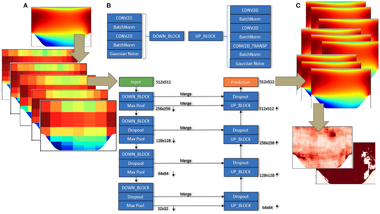
Figure 1. A schematic of the proposed super-resolution framework. (A) Shows the creation of an augmented and downsampled input feature space from the input field using Voronoi tessellation, (B) shows the chosen U-net architecture containing additional dropout and batch normalization layers, and (C) shows the ensemble of super-resolved field outputs along with the estimated uncertainties and error bounds.
2.2. Adversarial training
Generative Adversarial Networks (GANs) are a type of deep learning algorithm that are used to generate new, synthetic data samples that are similar to a training dataset. They consist of two neural networks: a generator network and a discriminator network. The generator network is trained to generate new, synthetic data samples, while the discriminator network is trained to distinguish between real and synthesized data samples. The two networks are trained together in an adversarial process, where the generator tries to generate samples that the discriminator cannot distinguish from real ones, and the discriminator tries to accurately identify whether a given sample is real or synthesized. GANs have been successful in a wide range of different types of super-resolution tasks (Deng et al., 2019; Bode et al., 2021; Güemes et al., 2022).
PatchGAN (Isola et al., 2016) is a kind of GAN model that employs a special type of discriminator network which only penalizes structure at the scale of local image patches and has proved to be helpful in the generation of high-quality, realistic images. The primary difference between a PatchGAN and a regular GAN discriminator is that while the regular GAN maps from a N × N image to a single scalar output, that indicates “real” or “fake,” the PatchGAN runs a k × k patch convolutionally across the N × N image to produce a d × d array of outputs Y (d = N − k + 1 with no padding and stride=1) where each Yij indicates whether the ijth patch in the original image is “real” or “fake.” If needed, a final scalar output can be obtained by averaging the responses in the output array. However, by assuming independence between pixels separated by more than a patch diameter, this training paradigm is able to mimic a more sophisticated type of texture or style loss.
Both regular GAN and PatchGAN discriminators were explored in this work and the basic adversarial training workflow is detailed in Figure 2. The results reported in the following sections use the U-Net described above as the generator network, which compared favorably to using a randomly initialized CNN during development. The tessellated features are input into the U-Net generator, and the discriminator network is trained to predict the validity of the generated component velocity fields. Results from both residual and “weak”-PI losses are considered for a variety of mean flow geometries, which is explained more in the following section. All of the GAN results reported were obtained with a fixed learning rate of 1 × 10⁻⁴.

Figure 2. Overview of a single iteration of the training routine for the regular GAN model with weak-PI loss. The tessellated variables are input into the generator network (see Figure 1), which can utilize a combined residual and physics-informed loss function. The generated SR output is checked by the discriminator to be a real or fake flow, and the entire model is trained iteratively in this adversarial fashion.
2.3. Approximate bayesian techniques for uncertainty estimation
The predictive uncertainty of a deep learning (DL) model usually consists of two parts—the epistemic (model uncertainty) and aleatoric (data uncertainty). Aleatoric uncertainty is an inherent property of the data distribution that can be attributed to the stochasticity of the observations caused by noise and randomness. As such this type of uncertainty is considered irreducible. Epistemic uncertainty refers to the model's uncertainty due to the lack of relevant, annotated, high-quality training data. Models are always expected to have high epistemic uncertainty when the training data is either limited in quantity or when it is rich in quantity but poor in informative quality, and thus offers inadequate knowledge about the actual use cases.
Bernoulli dropout was originally (and still is) used for regularizing a model to perform better on unseen scenarios (Wager et al., 2013; Srivastava et al., 2014). This methodology multiplies the output of each neuron by a binary mask drawn from a Bernoulli distribution, thus effectively deleting a random set of weights in the neural network during each epoch of training, which forces the network to create multiple pathways to make the correct inference. Several studies have shown dropout to be an effective technique to reduce overfitting while training deep neural networks. However, Gal and Ghahramani (2016) showed that Monte Carlo samples of the posterior distribution for a specific input can be efficiently obtained at test time by performing several stochastic forward passes while sampling different dropout masks for each prediction. They showed that any deep network trained with dropout is an approximate Bayesian model, and estimates of the epistemic uncertainty can be obtained by computing the variance of multiple predictions on the same input with different dropout masks, thus avoiding expensive Monte Carlo (MC) computations. This so-called Monte Carlo dropout (MCD) technique was also adopted in this work to estimate the epistemic uncertainty of the trained SR model with minimal changes to the network architecture and training algorithm. For each downsampling and upsampling block, the MCD rate was 10% (meaning 10% of the neurons were turned off during any given forward pass), with the exception of the lowest resolution upsampling layer which had a dropout rate of 50%. While 50% is much higher than the typical rates used in dropout-enabled studies, the skip connections present in the U-Net architecture alleviated the need to retain and transmit all important information between consecutive block layers.
Many modern neural network architectures have adopted another regularization technique called batch normalization (Ioffe and Szegedy, 2015) (BN) due to its ability to stabilize learning with improved generalization. BN is a neuron-wise operation to standardize the input distribution for each neuron in a particular layer of a deep network. For instance, in a fully connected layer, the input u for a neuron is transformed by the relation . Here the statistical measures (expectation and variance) are calculated over mini-batches during training and over the entire training set during evaluation or testing. Thus, effectively the inference for a sample x during training becomes a stochastic process that is dependent on other samples in the mini-batch. This stochasticity was utilized in Teye et al. (2018) to show that training using BN can also be cast as approximate Bayesian inference, similar to training with dropout, and this allows the estimation of epistemic uncertainty using a technique called Monte Carlo batch normalization (MCBN). In this strategy, during inference for a given query, several mini-batches are constructed by taking random samples to accompany the query. The mean and variance of the ensemble of outputs are then used to estimate the predictive distribution.
In this work, batch normalization layers were used in addition to dropout to serve the dual purpose of further enhancing the generalizability and robustness of the trained SR model, while also facilitating the uncertainty estimation of the trained model using an ensemble of predictions. For the cases where training data was extremely limited, multiple realizations of each input sample were generated to artificially augment the training dataset in order to enable the use of batch normalization. Because of the asymmetric nature of the physical systems studied here, a unique data augmentation method was adopted. In this process, sensor measurements are first projected onto a 512 × 768 grid using Voronoi tessellation to create a high-resolution estimate of the flow field represented, following Fukami et al. (2019, 2021). In the second step, several “downsampled,” uniformly gridded representations (n being the sensor count, 49 ≤ n ≤ 225) of the high-resolution tessellated field are generated to imitate lower sensor counts or sparse data, thus augmenting the initial dataset. Eventually, the lower-resolution instances are used for training the model while the instance with the highest sensor count is used for testing and validation. These artificially simulated sensor configurations not only enriched the training set but also allowed the successful sampling of multiple mini-batches for the implementation of MCBN. While this data augmentation strategy was uniquely appropriate for the problems explored in this work, several other related techniques of artificial data augmentation which exploit various symmetries of the physical systems or the geometrical configurations may be relevant for other problems.
3. Numerical experiments
Training and testing consisted of several different applications, with experiments done to highlight the capability of the model to bound the prediction error for unseen testing scenarios with the estimated epistemic uncertainty, as derived from a combination of Voronoi tessellation-based upsampling, MC batch normalization, and MC dropout. Numerical examples were selected from a variety of domains, including multi-geometry Reynolds-Averaged Navier Stokes (RANS) mean fluid flow, global sea-surface temperature, and global soil moisture datasets. This was done to explore and demonstrate the applicability of the model to different dynamical and realistic physical systems. The highest-resolution gridded representation used for training or inference in this study was a uniform sensor grid of 15 × 15 sensors. These input features were super-resolved to a 512 × 756 grid in the multiple geometry flow cases and to a 180 × 360 grid in the time-dependent geospatial datasets. The model performance for each numerical example was evaluated on not only the quality of the super-resolution reconstruction but also the ability of the uncertainty estimate (two times the standard deviation of the ensemble of predictions) and the range of the ensemble predictions to bound the error during inference. Implementation details and methodologies tested differed slightly from case to case, as will be discussed in Section 4.
3.1. Flow over varied geometries
Different combinations of network architectures and loss functions were evaluated for different surface geometries from the time-averaged Direct Numerical Simulation (DNS)/RANS dataset of McConkey et al. (2021). Table 1 shows the different cases of McConkey et al. (2021) used in the present study. Three different geometries were chosen: (1) Periodic Hills (PH) that had five realizations of varying steepness but a constant Reynolds number (Re) of 5, 600; (2) a Parametric Bump (PB) with five realizations of different height and a Re between 13, 260 and 27, 850; and (3) a Converging-Diverging channel (CD) with two realizations with a varying Re of 12, 600 and 20, 580. Nine of these twelve mean-flow scenarios were employed for training and the remaining three were reserved for testing. Due to the relatively small training set a low-shot training process was necessary.
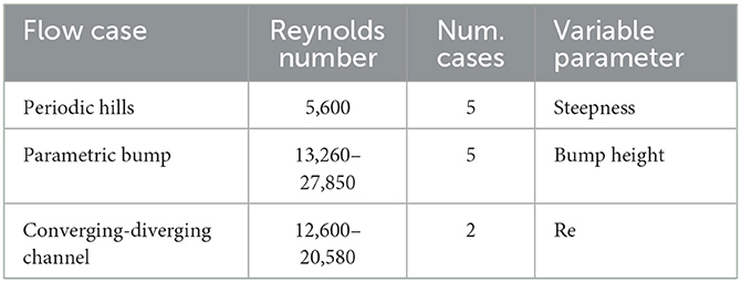
Table 1. Different mean flow cases extracted from the McConkey et al. (2021) dataset with their corresponding Reynolds numbers, number of cases, and variable parameters.
To supplement the low sample count, a Voronoi tessellation-based data augmentation strategy was adopted, as described in Section 2. The sensor locations were designed to follow a logarithmic scale in the y-direction starting from the bottom wall, with uniform spacing in the x-direction, and had no local refinement near the surface features. While following this gridded approach to generate the downsampled training instances, if a sensor was placed outside the flow domain (e.g., within a hill), the associated velocity fields were assigned zero values. Training time was approximately 1 h on an NVIDIA Titan V RTX graphics processing unit (GPU).
To further address the issue of an extremely limited training set (nine flow scenarios), a hybrid learning strategy was explored by enforcing the principle of mass conservation, also known as the continuity equation, as a physics-informed (PI) constraint to the loss function while training the neural network models. As shown in Equation (1), a penalty term was added to the loss function by taking the absolute value of the divergence of the velocity vector.
This combined loss, referred to as weak-PI loss for the remainder of the paper, was used as a methodology to perform physics-guided training of the deep learning models in low-resource paradigms by ensuring that the manifold of possible solutions was constrained by known physical laws. The use of only the conservation of mass principle instead of the full system of governing equations was a judicious choice that allowed more flexibility in the training process. The continuity constraint requires only two or three components of velocity as input and outputs the same variables at a higher resolution, thus being inherently more similar to the true spirit of single-image super-resolution tasks. Considering the full system of Navier-Stokes equations as a PI constraint would have required the other two coupled variables, pressure, and density, to also be included in the input feature space and in the output labels, thus significantly increasing the computational and data burden.
Two different approaches were studied to implement the weak-PI loss during training. The first approach involved numerical approximation of the divergence term by computing second-order finite difference derivatives of the output velocity fields. Despite the limitations in accuracy owing to the use of finite difference approximations, this approach was simpler to implement in an existing residual-loss architecture and required very minimal information about the spatial discretization of the computational domain. In the second approach, the well-known automatic differentiation technique utilized by the PINN method and its variants (Bode et al., 2021; Karniadakis et al., 2021; Yang et al., 2021) was adopted. In this technique, the neural network model requires information about the spatial discretization in order to compute a high-precision numerical approximation of the spatial derivatives of the output fields using automatic differentiation during every iteration of the training loop. However, in our numerical experiments with the weak-PI loss, the second approach provided negligible benefit over the first one despite requiring significantly more memory and training time. Hence, all of the numerical results presented in this work were obtained using the first approach.
The models were tested simultaneously on all three geometries, using the most extreme example for each case (periodic hills: steepest hill; parametric bump and converging-diverging channel: highest Reynolds Number [27,850 and 20,580, respectively]; details are provided in Table 1). An ensemble of size 100 was generated for each test example using either the U-Net or the GAN-based model, both with and without the weak-PI loss term. In an effort to keep input fields to a minimum and to minimize computational complexity, only the tessellated versions of the Ux and the Uy components of the flow velocities were used as input features along with a “wall distance” metric, that returns the distance of a sensor location from a wall.
3.2. Soil moisture
Based on the results of the multi-geometry mean flow example, the architecture and loss function combination with the lowest RMSE and uncertainty bounding percentage was also applied to a global soil moisture (SM) dataset (Orth, 2021), that provides soil moisture snapshots at three depths (0 − 10 cm, 10 − 30 cm, 30 − 50 cm) at a 0.25° spatial resolution and at a daily temporal resolution spanning the years 2000 − 2019. As detailed in Orth (2021), this dataset was created using in-situ moisture measurement data from more than 1, 000 stations around the world. These measurements, along with dynamic and static meteorological measurements, were used to train a Long short-term memory (LSTM) neural network. This network was then used to infer global soil moisture fields daily in response to dynamic changes in meteorological measurements.
Similar to the previous case, several sparse representations were derived from each SM snapshot using Voronoi tessellation to produce different sensor configurations for the training set. During this process, all grid cells that were closest to any sensor not located on the land surface were assigned a value of zero soil moisture. The model was trained on a subset (due to memory constraints) of daily SM snapshots from years 2000 − 2016 and tested on 16 snapshots evenly sampled from 2019. Training time was approximately 3 h on the system described above. Also similar to the previous mean flow example, the model output statistics for each test case were computed using an ensemble size of 100. Tessellated sparse representations of the soil moisture snapshots as well as a land-sea mask were used as input features. The purpose of the land-sea mask was to focus the learning process only on the land surface and to ensure that the artificially labeled sensors on the sea surface did not bias the RMSE calculations.
3.3. Sea-surface temperature
The third and final numerical example was the National Oceanographic and Atmospheric Association's (NOAA) Optimum Interpolation (OI) SST V2 weekly mean temperature dataset (Reynolds et al., 2002, 2007). This dataset provides weekly mean sea-surface temperature (SST) snapshots on a 1° × 1° resolution global grid (180 × 360 cells) for the years 1981 − 2022. The SST snapshots were augmented and downsampled using Voronoi tessellation to generate a collection of different sensor configurations for the training set. Following the same principle as in the previous examples, sensors and associated closest cells that fell on land were assigned a temperature value of zero.
The model was trained on weekly mean SST snapshots for the years 1991 − 2015 and tested on 17 snapshots evenly sampled from the year 2019. Training time was approximately 3 h on the system described above. As in the previous example, tessellated sparse representations of the SST snapshots and a land-sea mask were provided as input features to the model. In addition to evaluating the quality of the super-resolution reconstruction and the associated uncertainty estimates, the SST dataset was also used to study the effect of ensemble size on the model prediction statistics. Each test case was evaluated using a series of ensemble sizes from 100 to 800 and the comparative results will be discussed in the following Section 4.
4. Results
4.1. Flow over varied geometries
The performances of different combinations of network architecture and loss function implementation for the extrapolatory case of each mean flow geometry is reported in Table 2. There are substantial differences in two key metrics: (1) the super-resolution reconstruction accuracy, with mean absolute errors (MAEs) ranging from 0.016 to 0.134, and (2) the ability to bound the prediction error during out-of-sample inference using the uncertainty estimate, with error bound (EB) percentages, (defined as the percentage of points in the output field variable where the error is less than the uncertainty estimate), ranging from 22% to 93%. The U-Net with residual loss had the lowest MAEs for the periodic hills (PH) and parametric bump (PB) cases (MAE = 0.016 and 0.019, respectively) and the second lowest MAE=0.055 for the converging-diverging channel (CD) case. The U-Net with residual loss also performed the best in terms of bounding the error with the uncertainty estimate (EB = 93%) for the converging-diverging channel case. Training the U-net with the continuity-based weak-PI loss performed better than any other model, although only marginally, in terms of bounding the error with the uncertainty estimate (EB = 77%) for the PB case, whereas it was significantly worse for every other case.

Table 2. The mean absolute errors (MAEs) and error bound (EB) percentages for the extrapolative test cases of different geometric flow fields from the mean flow example, using every combination of model architecture and loss function type.
The regular GAN model, using the U-Net architecture as the generator network and a standard scalar-valued discriminator, didn't perform as well as the U-Net trained with either of the loss functions. In particular, the regular GAN trained with the weak-PI loss had the lowest reconstruction accuracy (MAE = 0.134) for the CD case and the lowest error bounding percentage (EB = 22%) for the PB case, among all the trained models (see Table 2). However, it is worth noting that the CD test case was the most extreme low-shot learning scenario, with both training and test datasets comprising only one mean flow case each.
The PatchGAN model, trained with the array-valued discriminator and a residual loss function, significantly outperformed the regular GAN model, trained with residual loss, in all of the cases. In particular, the PatchGAN model trained with residual loss had the highest error bounding percentage (EB = 85%) for the PH case, and the highest reconstruction accuracy (MAE = 0.046%) for the CD case among all of the models. Even for the PB case, it was one of the best-performing models. However, the PatchGAN model when trained with the weak-PI loss performed significantly worse. In fact, the regular GAN and the PatchGAN models when trained with the weak-PI loss were comparably the two of the worst-performing models in all of our numerical tests.
4.2. Soil moisture and sea-surface temperature
Based on the results of the mean flow example, further numerical tests were carried out using two non-fluid-flow examples, namely the multi-layer global soil moisture (SM) and the sea-surface temperature (SST) datasets, as outlined in Section 3. Table 3 presents a comparative summary of the performance of the best model, namely U-net trained with residual loss, on all three datasets. This quantitative comparison is presented in terms of the following metrics to measure accuracy—the normalized root mean square error (RMSE), the normalized MAE, and the normalized prediction bias (i.e. the difference between the mean of the predicted ensemble and the true target value). Additionally, two more metrics are evaluated to measure the quality of the uncertainty estimate— the error bound (EB) i.e. the percentage of points where the error is bounded by the uncertainty estimate, and the value bound (VB), defined as the percentage of points where the true target value is bounded by the maximum and minimum values of the ensemble. The RMSE and MAE values for both the SST and SM examples (0.016, 0.026, and 0.012, 0.017, respectively) were lower than the corresponding values for the mean flow example averaged over all the different geometries. Also, the biases for both the SST and SM examples (0.006 and 0.002 respectively) were about an order of magnitude lower than the mean flow example. In contrast, the EB fell from 82% for the mean flow example to 74 and 66% for the SST and SM examples, respectively. However, while the improvement from an EB of 82 to a VB of 84% was minimal for the mean flow example, the corresponding increment for the SST and SM examples were substantial, namely from 74 to 91% and from 66 to 79%, respectively.
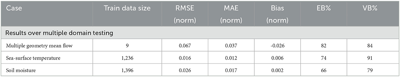
Table 3. The root-mean-squared error (RMSE), mean absolute error (MAE), bias, error bound (EB) percentage, and value bound (VB) percentage for the U-net residual model when trained and tested on the multiple-geometry mean flow, sea-surface temperature, and soil moisture datasets.
5. Discussion
In this work, a new method is proposed that utilizes a combination of Voronoi tessellation, MC batch normalization, and MC dropout to generate a high-quality super-resolution field reconstruction from sparse sensors for different dynamical physical systems. The method was tested on several numerical examples including both fluid flow and non-flow scenarios. When used to model mean flow fields across different geometric configurations, a U-net inspired architecture trained with a residual loss function was found to be more effective than a similar architecture trained with a physics-informed loss function, and also an adversarially trained generative model with an array-valued PatchGAN discriminator (Table 2).
An estimate of the epistemic uncertainty of the model was computed by returning two times the standard deviation of the ensemble of predictions at each location. The uncertainty estimate of the model was successful at bounding the error of the prediction mean (EB = 82%) in the low-shot learning environment for the multiple geometry mean flow cases from the McConkey et al. (2021) dataset, as listed in Table 1. When applied to the SST and the SM datasets, the percentage of points in the test set where the error was bounded by the uncertainty dropped to 76 and 67%, respectively. However, it was observed that the target values were still bounded by the range of the predicted ensemble, as measured by a VB of 91 and 79%, respectively.
Figure 3 shows a graphical representation of the relationship between error during inference and the estimated epistemic uncertainty of the model (left column) as well as a distribution of the model's prediction and target values at each pixel (right column). The scatter plots in the right column show that overall there was very good agreement between the model predicted and the true target values for all three numerical examples. However, there were some outliers in the multiple-geometry mean flow cases that are concentrated near the scalar extremes of the prediction values. In the left column of Figure 3, the scatter plots of the error and the uncertainty show that a vast majority of pixels in each example were located inside the red cone, indicating a bounding of the error by the estimated uncertainty. However, there were some noticeable differences in the distribution of errors and uncertainties for the three different examples. The ensemble of mean flow predictions was seen to be skewed toward a negative bias, which resulted in nearly all pixels with a positive bias being easily bounded by the uncertainty estimates, while some of the pixels with extreme negative biases fell outside the bounding red cone in the top left plot. The ensemble of predictions in the sea-surface temperature example was also skewed in a similar fashion but in the opposite direction. In other words, the positively skewed ensemble led to a majority of pixels with a negative bias being bounded by the uncertainty estimate but failed to bound some of the pixels with the most pronounced positive biases in prediction. The three-layer soil moisture example had a much more symmetric distribution in the scatter plot of error vs. uncertainty (bottom left plot) which meant that an almost equitable number of pixels with positive and negative biases were bounded by the uncertainty estimates. However, unlike the mean flow and SST examples, the prediction ensemble of the SM example had a large number of pixels with extremely low values of uncertainty, and thus a subset of these pixels were found to have errors that weren't bounded by the uncertainty estimates. These effects and others are discussed in more depth with specific examples in Sections 5.1, 5.2.
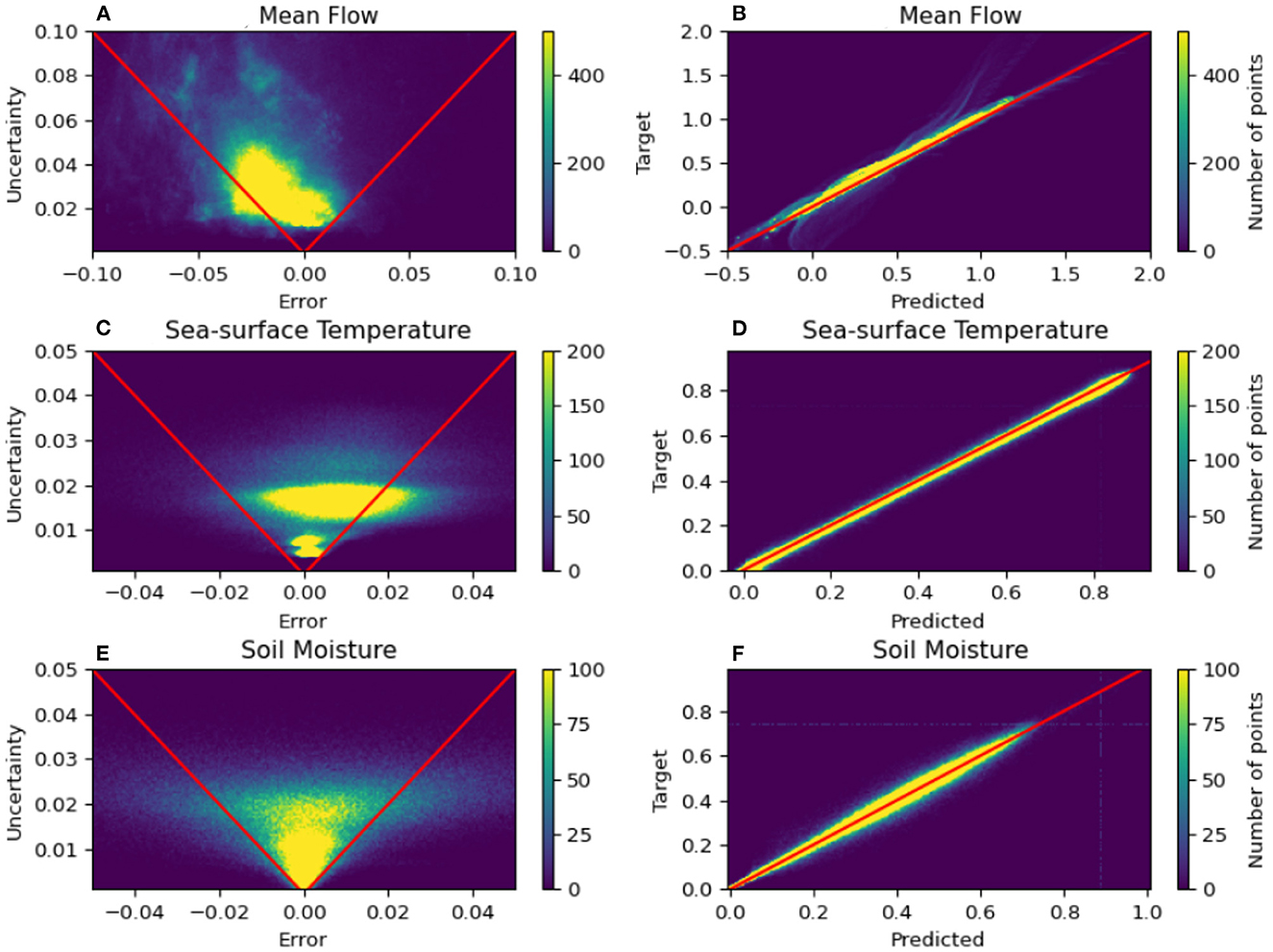
Figure 3. Summary of the relationship between the epistemic uncertainty and the prediction error for the mean flow (A, B), sea-surface temperature (C, D), and soil moisture (E, F) examples. Figures in the left column show the correlation between the prediction error and the estimated uncertainty for each of the examples while the figures in the right column show the correlation between the predicted and the true target values for the same example. The areas of the figures in the left column that fall within the red cone contain the points in the super-resolved fields where the uncertainty estimate bounds the prediction error. The red lines in the right column signify the points where the predicted and the target values match.
5.1. Mean flow accuracy and uncertainty quantification
The U-Net model with a residual-based loss performed better than the U-Net model trained with the weak-PI loss, as well as the regular GAN and the PatchGAN models both with and without the weak-PI loss. The negligible benefits of training the different models with either form of the continuity-based weak-PI loss (see Table 2) demonstrates that training with simply a residual loss function can be effectively used for super-resolution reconstruction and error estimation in problems where the governing physical laws may not be known. However, while the weak-PI loss function did not improve the results of our tests significantly, it also had a minimal negative impact on the ability of the model-predicted uncertainty to bound the error during inference. This leaves open the possibility that similar forms of physics-informed loss functions could improve results in other computational fluid flow problems. Specifically, an interesting extension of the study conducted here would be to constrain the learning process by enforcing the full set of relevant governing equations including the conservation of momentum, as they arise in the incompressible Navier-Stokes or the Reynolds averaged Navier-Stokes (RANS) equations.
Additionally, when the low-shot mean flow model was trained exclusively on samples involving a single geometry, the phenomenon of overfitting led to a reduction in the accuracy of the super-resolved output for extrapolatory test cases. Moreover, it also caused the model to erroneously overestimate its certainty, thus generating an ensemble of predictions with a very low variance that was not sufficient to bound the prediction error. Combining data samples from multiple geometries of the mean flow example in the training dataset improved the ability of the model to accurately extrapolate on test cases, and also increased the effectiveness of using an uncertainty-based bound to track the error in inference. It should be noted that an additional input feature in the form of a “wall distance” metric was necessary when data samples from multiple geometries were used for training the model. This “wall distance” metric measured the distance of a pixel from the closest boundary in any given geometry, and was introduced as an additional input channel. Moreover, additional care was taken to ensure that the state variables (input features) arising from flows with different geometric and flow parameters such as steepness, bump height and Reynolds number, were appropriately scaled before training and inference.
Specific examples can help highlight the capacity of the uncertainty of the model to estimate regions of increased error. Test results using the U-net model trained with the residual loss function for mean flow over three different geometries are depicted in Figure 4. Figures 4A–C show the tessellated input fields, the target fields, and the predicted flow fields, respectively. Figure 4D depicts the relative prediction error fields, Figure 4E shows the relative uncertainty fields, and Figure 4F uses a binary color-coded visualization format to differentiate the pixels where the estimated uncertainty bounds the error (red) from the ones where it doesn't (blue). The results across these different geometries (PH, PB, and CD) highlighted the natural variance that the U-Net model outputs when looking at different flow fields. In each case, the relative error field (Figure 4D) was found to qualitatively emulate the same spatial patterns observed in the corresponding epistemic uncertainty field (Figure 4E). Regions of the flow field with a high amount of mixing such as the wake regions downstream of the obstructing features were consistently well represented in the relative uncertainty fields as regions of significantly high uncertainty (> 20%), whereas regions with nearly laminar flow characteristics, away from the obstacle, were predicted to have much lower uncertainty (< 5%). While some of the flow regions with higher relative error were not bounded by the uncertainty (Figure 4F), in most cases this could be attributed to regions with very low levels of both error and epistemic uncertainty. The super-resolution reconstruction results for the CD case (Figure 4, column three) were the worst among the three. This could be explained by the extreme lack of data, with only one flow instance (Re = 12,600) available for training and one (Re = 20,580) available for carrying out tests. Not surprisingly, the estimated epistemic uncertainty of the CD case was much higher than the other two cases and consequently, the percentage of pixels where the error was bounded by the uncertainty was the highest for this case (EB = 93%). On the other hand, the PatchGAN model outperformed the U-Net residual loss model in the CD case (U-net MAE = 0.055 and PatchGAN MAE = 0.046). These results indicated that the stronger structural relationships enforced by the PatchGAN discriminator during training could potentially be helpful for training these types of models in situations with very limited data, however further research is needed to better understand these effects.
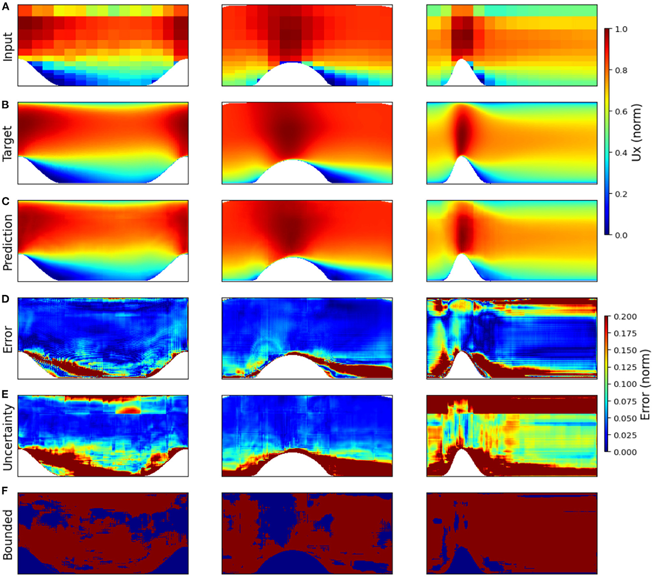
Figure 4. Results for the different test cases of the mean flow example taken from McConkey et al. (2021). The dimensionality and aspect ratio of each case varied significantly, and are shown as dimensionless reconstructions on a 512 × 756 grid for ease of visualization. The x component of velocity, Ux, is shown, with the tessellated input (A), the target values (B), and the predicted values (C) all normalized between 0 and 1. The relative error (D) and relative uncertainty (E) are shown for each case. Finally, the areas where the epistemic uncertainty bound the observed error are shown in a binary color-coded format (F) where red indicates a pixel is bounded, and blue indicates it is not.
5.2. Non-flow accuracy and uncertainty quantification
5.2.1. Soil moisture
The multi-layer SM dataset (Orth, 2021) provided an opportunity to apply this methodology on a different, realistic physical system with a much richer set of training and testing data. Figure 5 shows the results obtained using the U-net residual loss model on a data sample from the test set. Figures 5A–C in the top row show the tessellated input field, the super-resolved soil moisture field, and the high-resolution target soil moisture field, respectively, as false color composite images using the standard visual RGB band range (red, green, and blue). The first layer (0–10 cm depth) is represented by the red channel, the second layer (10–30 cm depth) is represented by the green channel, and the third layer (30–50 cm depth) is represented by the blue channel. Darker regions in each color band represent lower values of soil moisture, while lighter regions indicate more moisture, and different intermediate hues indicate moisture imbalance by depth. Even though the tessellated input field was extremely sparse and contained many regions with zero soil moisture content across all three layers as denoted by the black colored blocks in Figure 5A, the model prediction (Figure 5B) showed excellent agreement with the target soil moisture field (Figure 5C). The relative error fields for the three soil layers as depicted in descending order of depth in Figures 5D–F, respectively, showed a distinct trend of decreasing moisture content with increasing depth. This was intuitively expected given the understanding that the seasonal variation in soil moisture content typically reduces with increasing depth below the surface.
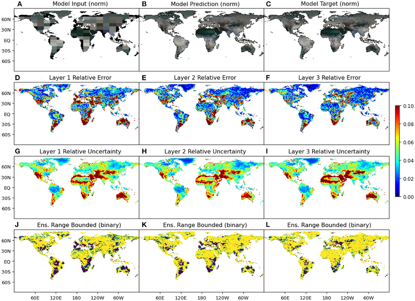
Figure 5. Results for an unseen test snapshot from the three-layer global soil moisture dataset (Orth, 2021). The tessellated input (A), the model prediction (B), and the model target (C), all normalized between 0 and 1, are depicted by a false-color composite plot with the moisture content in each layer being represented by an individual channel of an RGB image. Thus, the whole spectrum from darker to lighter colors is used to denote lower to higher moisture content, respectively, across all three layers. (D–F) Show the relative errors, (G–I) show the relative uncertainty fields, and (J–L) show the areas where the target value is bounded by the model ensemble prediction for the layers 0−10 cm, 10−30 cm, and 30−50 cm in depth, respectively.
Semi-arid regions (such as the Australian Outback, Mongolia, the Middle East, South Asia, and large parts of Africa) are known to experience the largest variations in the dryness of climate (aridity index of 3–10) over the course of a given year (Lin, 1999). These large variations manifested as significant temporal changes in soil moisture content across the training dataset which, in turn, led to a high amount of variance in the ensemble of model predictions for these regions. Combined with the low absolute values of moisture in many of these regions for the test instance presented in Figure 5C, this led to large amounts of relative uncertainties, as shown in Figures 5G–I in descending order of depth. The absolute uncertainty of each layer also decreased with depth, but less than the corresponding reduction in error. This led to an increase in the layer-wise area where the target moisture value was bounded by the predicted ensemble, as shown in Figures 5J–L using a binary color-coded format with yellow representing the pixels that were bounded and purple representing the ones that weren't. In this example, the points with higher relative error and relative uncertainty were primarily located in arid and semi-arid zones and in areas of the input field where the soil moisture content was estimated to be zero due to the effect of tessellation across land-sea boundaries (colored black in Figure 5A). Hyper-arid zones, such as the Sahara Desert, had extremely low soil moisture variations in the training dataset, and subsequently, showed extremely low relative errors and uncertainties. The soil moisture content in the uppermost layer (0 − 10 cm in depth) is expected to be the most sensitive to changes in weather patterns, and consequently, underwent large variations in the training set. As a result, both the reconstruction accuracy (Figure 5D) and the percentage of points where the target soil moisture value was bounded by the range of the prediction ensemble (Figure 5J) were observed to be the lowest in the uppermost soil layer. While the regions with the highest error (>|0.02|) had a strong positive correlation with higher uncertainty values ((> |0.015|), the magnitude of the uncertainty was not always sufficient to bound the target moisture value.
5.2.2. Sea-surface temperature
Finally, the U-net with residual loss methodology was evaluated on the global sea-surface temperature dataset from NOAA (Reynolds et al., 2002, 2007). Figures 6A–F show the super-resolution results on an extrapolatory test snapshot of the weekly mean sea surface temperature for the 33rd week of 2019. The contours of the reconstructed field (Figure 6B) exhibit very close agreement with those of the target field (Figure 6C), even on subgrid-scale features, despite the large information gap with the lower-resolution grid of the tessellated input field (Figure 6A). Most of the finer scale details were well resolved, as demonstrated by a pixel-wise relative error of less than 5% for most of the non-polar waters, although the contours of the predicted field were noticeably smoother than those of the target field. According to the relative error field in Figure 6D, areas with high relative errors, especially in warmer waters, were primarily concentrated around areas of high gradient in the tessellated sensor measurements (Figure 6A). However, high relative error regions were also observed in coastal areas, such as in coastal Eastern Asia and Western North America, and were caused by the effect of tessellation on a coarse grid across land-sea boundaries combined with large gradients in the near-shore sea surface temperatures.

Figure 6. Results for an unseen test snapshot from the NOAA sea-surface temperature dataset (Reynolds et al., 2002, 2007). (A) Shows the tessellated input field, (B) the contours of the predicted temperature field, (C) the contours of the target temperature field, (D) the relative error field, (E) the relative uncertainty field, and (F) the regions where the range of the predicted ensemble bounds the prediction error, represented as a binary color-coded plot where red indicates a pixel is bounded, and blue indicates it is not.
The estimated epistemic uncertainty of the model (Figure 6E) bounded the observed error to a large extent (EB = 76%), whereas the percentage of pixels where the full ensemble range bounded the target value (Figure 6F) was significantly higher (VB = 85%). The uncertainty of the model was consistently low for temperate waters with normalized temperatures ranging between 0.3 and 1.0 (roughly 14° C to 31°C), as reflected in the nearly constant relative uncertainty values between latitudes 30S to 30N (see Figure 6E). The steep increase in both the relative error and the relative uncertainty values in the polar regions could be primarily attributed to the sharp drop in the magnitude of the sea surface temperatures while the absolute values of error and uncertainty exhibited a more gradual decline. Moreover, the trained model showed a consistent change in the variability of the predicted ensemble that was typically proportional to the changes in the prediction error while keeping the magnitude of the error low almost throughout the domain. This amounted to the trained model being highly effective in bounding the target values within the range of the predicted ensemble, as reflected in the highest value of VB = 85% among all the numerical examples (see Figure 6F).
To understand the characteristics of the distribution of predictions generated by the framework, the ensemble of predictions for three individual pixels across three different temperature ranges (approximately 0.15, 0.41, and 0.83) were studied. Figures 7A–F shows the histograms of the model predictions obtained either with an ensemble of size 100 (Figures 7A, C, E) or with an ensemble of size 300 (Figures 7B, D, F). In each figure, the red vertical line marks the target value for each pixel while the black curve depicts the probability density function defined by the ensemble statistics assuming it follows a normal distribution. The global coordinates of the chosen pixels are denoted by three black dots on the super-resolved prediction field in Figure 7G. Figures 7A, C, E, show that given the choice of the numerical example (SST) and the modeling framework (U-net with residual loss), an ensemble size of 100 was sufficiently large for the model to adequately capture the temporal variability in the training dataset in order to generate an approximately normally distributed ensemble of predictions. Specifically, for Figure 7A, while the ensemble of size 100 did not show a peak of predictions around the mean (nearly uniform distribution between the values of 0.125 to 0.155), increasing the ensemble count to 300 (Figure 7B) showed a much more peaked distribution around the mean with the target value falling inside the two largest prediction bins. However, this barely affected the mean (0.137 vs. 0.136) or standard deviation (0.011 vs. 0.011) for the 100 and 300 ensemble count distributions, respectively. In Figure 7C, the smaller ensemble of predictions was more concentrated near the mean of the ensemble leaving the bins at the lower and higher ends of the distribution (centered at roughly 0.390 and 0.435) largely unpopulated. Increasing the ensemble size generated a more well-balanced distribution, as shown in Figure 7D. However, the ensemble mean (0.417) and std (0.008) remained unchanged up to three significant digits. The smaller ensemble for the final pixel location (Figures 7E, F) showed a similar under-representation at the lower end of the prediction range (0.79 − 0.81), creating a long (flat) tail. Similar to the other pixels, increasing the ensemble size allowed the model to generate a more well-balanced distribution of predictions that more closely resembled a normal distribution, without significantly altering the mean (0.825 vs. 0.826) or std (0.009 vs. 0.009) of the ensemble. Finally, Figure 7H shows the change in the percentage of points where (i) the uncertainty bounded the error (EB) and (ii) the range of ensemble predictions bounded the target value (VB) with the increase in ensemble sizes. Increasing the ensemble size from 5 to 100, showed a faster rate of improvement both for VB (< 50 to 80%) and a more gradual but significant rate of improvement for EB (≈60 to 74%). However, with any further increase in the ensemble size, there was very little improvement in the percentage of error bounded by uncertainty; at the same time, the percentage of points where the target value is bounded by the range continued to grow to over 90%, with very little degradation in the accuracy of the mean.
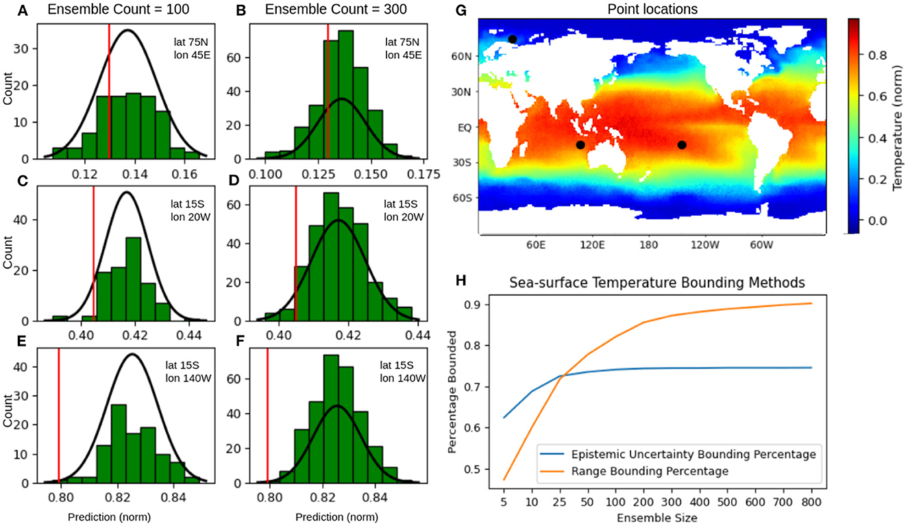
Figure 7. Analysis of the predicted ensemble for three different pixels of a random test sample from the NOAA Sea-Surface Temperature (SST) example. (A–F) Show a histogram of the model predictions at the indicated lat, lon coordinate, with the target value for that pixel represented by the vertical red line, (G) shows the location of these pixels as black dots superimposed on the prediction field, and (H) shows a plot of the percentage of pixels where the error is bounded by the epistemic uncertainty (blue) or the percentage of points where the target value lies within the range of ensemble predictions (orange) over the entire SST test set.
The previous analysis strongly indicated that with increasing ensemble sizes, the distribution of predicted values was starting to asymptotically converge, at least formally, to a Gaussian distribution. This implies an inherent reliability of the proposed MCBN/MCD ensembling methodology with repeated use, and this asymptotic behavior was observed for test datasets across multiple experimental domains. This analysis also indicated that for experiments and scenarios where computational resources and inference time are not limited, predictions with larger (>100) ensemble sizes had a higher chance of bounding the target value, providing a much better estimation of the range of possible values than looking at the epistemic uncertainty alone. Thus the reliability of the ensemble range to bound the error improved with additional computational time (> 90%). For extremely fast predictions and applications that require real-time prediction, the standard deviation of the ensemble provided more reliable results for the tested domains, especially when the ensemble size was less than 25.
5.2.3. Ongoing work
Ongoing work includes the exploration and application of this methodology for super-resolution modeling of wind tunnel experiments, currently being conducted at the U.S. Army Engineer Research and Development Center (ERDC) Synthetic Environment for Near-Surface Sensing and Experimentation (SENSE) wind tunnel facility. The immediate objective is to use super-resolution reconstruction to supplement and inform physical data collection in order to generate high-resolution data sets to support the development of generalized closure schemes for near-surface flows. This work will, in turn, support ongoing field observations and near-surface vegetated flow studies being conducted by the ERDC at the USDA Jornada Experimental Range in Las Cruces, NM, and the U.S. Army Corps of Engineers Field Research Facility in Duck, NC. Additional directions of future research at ERDC will involve using super-resolved soil moisture fields to support the generation of high-resolution maps from remote sensing and sparse in-situ observations. These maps are a key component of global hydrological analysis efforts that support a variety of missions, such as providing antecedent soil moisture conditions for flooding analysis in remote areas.
6. Conclusion
Using the U-Net architecture with a residual loss coupled with data augmentation and a Monte Carlo batch normalization and dropout scheme generates stochastic network predictions, such that for a statistically significant ensemble size the variability in the predicted distribution can be interpreted as epistemic uncertainty for super-resolution of dynamical physical systems. These estimates of epistemic uncertainty were shown to qualitatively follow inference error in all the problems and to successfully bound error in a majority of the cases for the low-shot multiple-geometry mean flow, soil moisture, and sea-surface temperature applications. However, results indicated that using the epistemic uncertainty itself may not always be the most reliable method for estimating inference error across all domains. By looking at the entire ensemble range, results were significantly improved with negligible degradation of the ensemble mean when compared to the target value, thus also showcasing the reliability of the MCD/MCBN ensemble-based estimation method. These results highlighted the utility of incorporating the epistemic uncertainty estimates with small ensembles (<25) for real-time prediction on computationally-intensive datasets. However, the observed ranges of predictions with larger ensembles (>25) were demonstrably more accurate in the characterization of possible inference values.
The methodology worked well for low-shot learning scenarios (only 9 training samples for the multiple-geometry mean flow example). Additionally, the incorporation of the continuity loss in the mean flow example produced comparable results in the uncertainty estimation (80 vs. 80%, 74 vs. 77%, and 93 vs. 78%; residual loss vs. weak-PI loss) for the periodic hills, parametric bump, and converging-diverging channel geometries, respectively. This shows the potential of similar deep ensemble-based frameworks constrained by appropriate physical laws for the estimation of target values and the range of possible errors when applied to dynamic physical systems with well-defined governing equations.
Data availability statement
The mean flow dataset is available at: https://www.kaggle.com/datasets/ryleymcconkey/ml-turbulence-dataset. NOAA Optimum Interpolation (OI) SST V2 data is provided by the NOAA PSL, Boulder, Colorado, USA, on their website at: https://psl.noaa.gov/data/gridded/data.noaa.oisst.v2.html. The soil moisture dataset is available at: https://doi.org/10.6084/m9.figshare.c.5142185.v1. All codes developed in this work will be publicly available on GitHub upon publication, accessible through the link https://github.com/erdc/SRUncertainty.
Author contributions
AC, PR-C, and SD handled dataset pipelines and network implementation and wrote sections of the manuscript. AC wrote the first draft of the manuscript. All authors contributed to the conception and design of the study, manuscript revision, read, and approved the submitted version.
Funding
Funding support for this research was provided by the U.S. Army Engineer Research and Development Center Fundamental Adaptive Protection/Projection Program (FAN: U4381188/Project: 500538) sponsored by the Assistant Secretary of the Army for Acquisition, Logistics, and Technology (ASA-ALT).
Acknowledgments
Ms. Pamela Kinnebrew was the program manager with the assistance of Mr. Justin Putnam for the fundamental research program sponsoring this work. The authors would like to acknowledge the technical support and input provided by Dr. Ian Dettwiller, Dr. Mathew Boyer, and Ms. Sandra LeGrand. The authors would also like to thank the internal reviewers at the ERDC for their time and constructive comments. Permission was granted by the Chief of Engineers to publish this information.
Conflict of interest
The authors declare that the research was conducted in the absence of any commercial or financial relationships that could be construed as a potential conflict of interest.
Publisher's note
All claims expressed in this article are solely those of the authors and do not necessarily represent those of their affiliated organizations, or those of the publisher, the editors and the reviewers. Any product that may be evaluated in this article, or claim that may be made by its manufacturer, is not guaranteed or endorsed by the publisher.
References
Abdar, M., Pourpanah, F., Hussain, S., Rezazadegan, D., Liu, L., Ghavamzadeh, M., et al. (2021). A review of uncertainty quantification in deep learning: techniques, applications and challenges. Inf. Fusion 76, 243–297. doi: 10.1016/j.inffus.2021.05.008
Apley, D. W., and Zhu, J. (2020). Visualizing the effects of predictor variables in black box supervised learning models. J. R. Stat. Soc. B Stat. Methodol. 82, 1059–1086. doi: 10.1111/rssb.12377
Atanov, A., Ashukha, A., Molchanov, D., Neklyudov, K., and Vetrov, D. (2019). “Uncertainty estimation via stochastic batch normalization,” in Advances in Neural Networks-ISNN 2019, volume 11554 LNCS, eds H. Lu, H. Tang, and Z. Wang (Cham: Springer International Publishing), 261–269.
Beck, A., and Kurz, M. (2021). A perspective on machine learning methods in turbulence modeling. GAMM-Mitteilungen 44, e202100002. doi: 10.1002/gamm.202100002
Blundell, C., Cornebise, J., Kavukcuoglu, K., and Wierstra, D. (2015). “Weight uncertainty in neural networks,” in Proceedings of the 32nd International Conference on International Conference on Machine Learning-Vol. 37, ICML'15 (Lille), 1613–1622.
Bode, M., Gauding, M., Lian, Z., Denker, D., Davidovic, M., Kleinheinz, K., et al. (2019). Using physics-informed super-resolution generative adversarial networks for subgrid modeling in turbulent reactive flows. arXiv preprint arXiv:1911.11380. doi: 10.48550/arXiv.1911.11380
Bode, M., Gauding, M., Lian, Z., Denker, D., Davidovic, M., Kleinheinz, K., et al. (2021). Using physics-informed enhanced super-resolution generative adversarial networks for subfilter modeling in turbulent reactive flows. Proc. Combustion Inst. 38, 2617–2625. doi: 10.1016/j.proci.2020.06.022
Carvalho, D. V., Pereira, E. M., and Cardoso, J. S. (2019). Machine learning interpretability: a survey on methods and metrics. Electronics 8, 832. doi: 10.3390/electronics8080832
Chen, R. T. Q., Rubanova, Y., Bettencourt, J., and Duvenaud, D. (2018). Neural ordinary differential equations. ArXiv 109, 31–60. doi: 10.1007/978-3-662-55774-7_3
Collins, A. M., Brodie, K. L., Bak, A. S., Hesser, T. J., Farthing, M. W., Lee, J., et al. (2020). Bathymetric inversion and uncertainty estimation from synthetic surf-zone imagery with machine learning. Remote Sens. 12, 3364. doi: 10.3390/rs12203364
Cortinhal, T., Tzelepis, G., and Erdal Aksoy, E. (2020). “SalsaNext: fast, uncertainty-aware semantic segmentation of LiDAR point clouds,” in Advances in Visual Computing, Lecture Notes in Computer Science, eds G. Bebis, Z. Yin, E. Kim, J. Bender, K. Subr, B. C. Kwon, J. Zhao, D. Kalkofen, and G. Baciu (Cham: Springer International Publishing), 207–222.
Deng, Z., He, C., Liu, Y., and Kim, K. C. (2019). Super-resolution reconstruction of turbulent velocity fields using a generative adversarial network-based artificial intelligence framework. Phys. Fluids 31, 125111. doi: 10.1063/1.5127031
Duraisamy, K., Iaccarino, G., and Xiao, H. (2019). Turbulence modeling in the age of data. Annu. Rev. Fluid Mech. 51, 357–377. doi: 10.1146/annurev-fluid-010518-040547
Dutta, S., Rivera-Casillas, P., Cecil, O. M., Farthing, M. W., Perracchione, E., and Putti, M. (2021a). “Data-driven reduced order modeling of environmental hydrodynamics using deep autoencoders and neural ODEs,” in Proceedings of the IXth International Conference on Computational Methods for Coupled Problems in Science and Engineering (COUPLED PROBLEMS 2021) (Stanford, CA: International Center for Numerical Methods in Engineering, CIMNE), 1–16.
Dutta, S., Rivera-Casillas, P., and Farthing, M. W. (2021b). “Neural ordinary differential equations for data-driven reduced order modeling of environmental hydrodynamics,” in Proceedings of the AAAI 2021 Spring Symposium on Combining Artificial Intelligence and Machine Learning with Physical Sciences (Barcelona: CEUR-WS), 1–10.
Dutta, S., Rivera-casillas, P., Styles, B., and Farthing, M. W. (2022). Reduced order modeling using advection-aware autoencoders. Math. Comput. Appl. 27, 34. doi: 10.3390/mca27030034
Fukami, K., Fukagata, K., and Taira, K. (2019). Super-resolution reconstruction of turbulent flows with machine learning. J. Fluid Mech. 870, 106–120. doi: 10.1017/jfm.2019.238
Fukami, K., Maulik, R., Ramachandra, N., Fukagata, K., and Taira, K. (2021). Global field reconstruction from sparse sensors with Voronoi tessellation-assisted deep learning. Nat. Mach. Intell. 3, 945–951. doi: 10.1038/s42256-021-00402-2
Gal, Y., and Ghahramani, Z. (2016). “Dropout as a Bayesian approximation: Representing model uncertainty in deep learning,” in Proceedings of the 33rd International Conference on International Conference on Machine Learning-Volume 48, ICML'16 (New York, NY), 1050–1059.
Gal, Y., Hron, J., and Kendall, A. (2017). “Concrete dropout,” in Proceedings of the 31st International Conference on Neural Information Processing Systems, NIPS'17 (Red Hook, NY: Curran Associates Inc.), 3584–3593.
Gao, H., Sun, L., and Wang, J. X. (2021). Super-resolution and denoising of fluid flow using physics-informed convolutional neural networks without high-resolution labels. Phys. Fluids 33, 1–34. doi: 10.1063/5.0054312
Goldstein, A., Kapelner, A., Bleich, J., and Pitkin, E. (2015). Peeking Inside the black box: visualizing statistical learning with plots of individual conditional expectation. J. Comput. Graph. Stat. 24, 44–65. doi: 10.1080/10618600.2014.907095
Güemes, A., Vila, C. S., and Discetti, S. (2022). Super-resolution generative adversarial networks of randomly-seeded fields. Nat. Mach. Intell. 4, 1165–1173. doi: 10.1038/s42256-022-00572-7
Ioffe, S., and Szegedy, C. (2015). “Batch normalization: accelerating deep network training by reducing internal covariate shift,” in Proceedings of the 32nd International Conference on International Conference on Machine Learning-Volume 37, ICML'15 (Lille), 448–456.
Isola, P., Zhu, J.-Y., Zhou, T., and Efros, A. A. (2016). Image-to-image translation with conditional adversarial networks. arXiv 1125–1134. doi: 10.1109/CVPR.2017.632
Jiang, W., Zhao, Y., Wu, Y., and Zuo, H. (2022). “Capturing model uncertainty with data augmentation in deep learning,” in Proceedings of the 2022 SIAM International Conference on Data Mining, SDM 2022, eds A. Banerjee, Z. Zhou, E. E. Papalexakis, and M. Riondato (Alexandria, VA: SIAM), 271–279.
Kadeethum, T., O'Malley, D., Fuhg, J. N., Choi, Y., Lee, J., Viswanathan, H. S., et al. (2021). A framework for data-driven solution and parameter estimation of PDEs using conditional generative adversarial networks. Nat. Comput. Sci. 1, 819–829. doi: 10.1038/s43588-021-00171-3
Kar, A., and Biswas, P. K. (2019). Fast Bayesian uncertainty estimation and reduction of batch normalized single image super-resolution network. arXiv. doi: 10.48550/arXiv.1903.09410
Karniadakis, G. E., Kevrekidis, I. G., Lu, L., Perdikaris, P., Wang, S., and Yang, L. (2021). Physics-informed machine learning. Nat. Rev. Phys. 3, 422–440. doi: 10.1038/s42254-021-00314-5
Kim, H., Kim, J., Won, S., and Lee, C. (2021). Unsupervised deep learning for super-resolution reconstruction of turbulence. J. Fluid Mech. 910:A29. doi: 10.1017/jfm.2020.1028
Krizhevsky, A., Hinton, G. E., Krizhevsky, B. A., Sutskever, I., and Hinton, G. E. (2017). Imagenet classification with deep convolutional neural networks. Commun. ACM. 60, 84–90. doi: 10.1145/3065386
Li, M., and McComb, C. (2022). Using physics-informed generative adversarial networks to perform super-resolution for multiphase fluid simulations. J. Comput. Inf. Sci. Eng. 22, 044501. doi: 10.1115/1.4053671
Liu, B., Tang, J., Huang, H., and Lu, X.-Y. (2020). Deep learning methods for super-resolution reconstruction of turbulent flows. Phys. Fluids 32, 025105. doi: 10.1063/1.5140772
Malinin, A., Mlodozeniec, B., and Gales, M. (2019). Ensemble distribution distillation. arXiv. doi: 10.48550/arXiv.1905.00076
Maulik, R., San, O., Jacob, J. D., and Crick, C. (2019). Sub-grid scale model classification and blending through deep learning. J. Fluid Mech. 870, 784–812. doi: 10.1017/jfm.2019.254
McConkey, R., Yee, E., and Lien, F. S. (2021). A curated dataset for data-driven turbulence modelling. Sci. Data 8, 1–14. doi: 10.1038/s41597-021-01034-2
Minka, T. P. (2001). A Family of Algorithms for Approximate Bayesian Inference (Ph.D. thesis). Massachusetts Institute of Technology, USA. AAI0803033.
Nori, H., Jenkins, S., Koch, P., and Caruana, R. (2019). InterpretML: A Unified Framework for Machine Learning Interpretability. ArXiv [Preprint].
Orth, R. (2021). Global soil moisture data derived through machine learning trained with in-situ measurements. Sci. Data 8, 170. doi: 10.1038/s41597-021-00964-1
Osband, I. (2016). “Risk versus uncertainty in deep learning: bayes, bootstrap and the dangers of dropout,” in Workshop on Bayesian Deep Learning, NIPS, 1–5.
Patel, D. V., Ray, D., and Oberai, A. A. (2022). Solution of physics-based Bayesian inverse problems with deep generative priors. Comput. Methods Appl. Mech. Eng. 400, 115428. doi: 10.1016/j.cma.2022.115428
Pearce, T., Leibfried, F., Brintrup, A., Zaki, M., and Neely, A. (2018). Uncertainty in neural networks: Approximately Bayesian ensembling. arXiv. doi: 10.48550/arXiv.1810.05546
Qian, Y., Forghani, M., Lee, J. H., Farthing, M., Hesser, T., Kitanidis, P., et al. (2020). Application of deep learning-based interpolation methods to nearshore bathymetry. arXiv. doi: 10.48550/arXiv.2011.09707
Raissi, M., Perdikaris, P., and Karniadakis, G. E. (2019). Physics-informed neural networks: a deep learning framework for solving forward and inverse problems involving nonlinear partial differential equations. J. Comput. Phys. 378, 686–707. doi: 10.1016/j.jcp.2018.10.045
Reynolds, R. W., Rayner, N. A., Smith, T. M., Stokes, D. C., and Wang, W. (2002). An improved in situ and satellite SST analysis for climate. J. Climate 15, 1609–1625. doi: 10.1175/1520-0442(2002)015and<1609:AIISASand>2.0.CO;2
Reynolds, R. W., Smith, T. M., Liu, C., Chelton, D. B., Casey, K. S., and Schlax, M. G. (2007). Daily high-resolution-blended analyses for sea surface temperature. J. Clim. 20, 5473–5496. doi: 10.1175/2007JCLI1824.1
Ronneberger, O., Fischer, P., and Brox, T. (2015). “U-net: convolutional networks for biomedical image segmentation,” in International Conference on Medical Image Computing and Computer-Assisted Intervention (Springer), 234–241.
Srivastava, N., Hinton, G., Krizhevsky, A., Sutskever, I., and Salakhutdinov, R. (2014). Dropout: a simple way to prevent neural networks from overfitting. J. Mach. Learn. Res. 15, 1929–1958.
Teye, M., Azizpour, H., and Smith, K. (2018). Bayesian uncertainty estimation for batch normalized deep networks. arXiv. doi: 10.48550/arXiv.1802.06455
Wager, S., Wang, S., and Liang, P. S. (2013). “Dropout training as adaptive regularization,” in Advances in Neural Information Processing Systems (Lake Tahoe, NV), 351–359.
Wang, L., Luo, Z., Xu, J., Luo, W., and Yuan, J. (2021). A novel framework for cost-effectively reconstructing the global flow field by super-resolution. Phys. Fluids 33, 095105. doi: 10.1063/5.0062775
Wang, S., Teng, Y., and Perdikaris, P. (2021). Understanding and mitigating gradient flow pathologies in physics-informed neural networks. SIAM J. Sci. Comput. 43, 3055–3081. doi: 10.1137/20M1318043
Wang, Y., and Ročková, V. (2020). Uncertainty quantification for sparse deep learning. arXiv. doi: 10.48550/arXiv.2002.11815
Wang, Z., Chen, J., and Hoi, S. C. (2020). Deep learning for image super-resolution: a survey. IEEE Trans. Pattern Anal. Mach. Intell. 43, 3365–3387. doi: 10.1109/TPAMI.2020.2982166
Yang, L., Meng, X., and Karniadakis, G. E. (2021). B-PINNs: Bayesian physics-informed neural networks for forward and inverse PDE problems with noisy data. J. Comput. Phys. 425, 109913. doi: 10.1016/j.jcp.2020.109913
Zayats, M., Zimoń, M. J., Yeo, K., and Zhuk, S. (2022). Super resolution for turbulent flows in 2D: stabilized physics informed neural networks. arXiv preprint arXiv:2204.07413. doi: 10.1109/CDC51059.2022.9992729
Keywords: super-resolution, machine learning, uncertainty, fluid flow, sea-surface temperature, soil moisture
Citation: Collins AM, Rivera-Casillas P, Dutta S, Cecil OM, Trautz AC and Farthing MW (2023) Super-resolution and uncertainty estimation from sparse sensors of dynamical physical systems. Front. Water 5:1137110. doi: 10.3389/frwa.2023.1137110
Received: 04 January 2023; Accepted: 23 February 2023;
Published: 14 March 2023.
Edited by:
Xiaofeng Liu, The Pennsylvania State University (PSU), United StatesReviewed by:
Haibin Chang, Peking University, ChinaKalyana Babu Nakshatrala, University of Houston, United States
Copyright © 2023 Collins, Rivera-Casillas, Dutta, Cecil, Trautz and Farthing. This is an open-access article distributed under the terms of the Creative Commons Attribution License (CC BY). The use, distribution or reproduction in other forums is permitted, provided the original author(s) and the copyright owner(s) are credited and that the original publication in this journal is cited, in accordance with accepted academic practice. No use, distribution or reproduction is permitted which does not comply with these terms.
*Correspondence: Adam M. Collins, YWRhbS5tLmNvbGxpbnNAZXJkYy5kcmVuLm1pbA==
†ORCID: Adam M. Collins orcid.org/0000-0003-3852-1509