The Budyko shape parameter as a descriptive index for streamflow loss

Increases in evapotranspiration (ET) from global warming are decreasing streamflow in headwater basins worldwide. However, these streamflow losses do not occur uniformly due to complex topography. To better understand the heterogeneity of streamflow loss, we use the Budyko shape parameter (ω) as a diagnostic tool. We fit ω to 37-year of hydrologic simulation output in the Upper Colorado River Basin (UCRB), an important headwater basin in the US. We split the UCRB into two categories: peak watersheds with high elevation and steep slopes, and valley watersheds with lower elevation and gradual slopes. Our results demonstrate a relationship between streamflow loss and ω. The valley watersheds with greater streamflow loss have ω higher than 3.1, while the peak watersheds with less streamflow loss have an average ω of 1.3. This work highlights the use of ω as an indicator of streamflow loss and could be generalized to other headwater basin systems.

Key points

- Sub-watersheds in the Upper Colorado River Basin respond differently to global warming due to the basin complex topography.

- Valley watersheds have had more streamflow loss than peak watersheds during dry years.

- The amount of streamflow loss can be quantified by the commonly used Budyko shape parameter.

1. Introduction

Global warming is causing streamflow loss in headwater basins globally (Immerzeel et al., 2010; Mastrotheodoros et al., 2020; Milly and Dunne, 2020). One of the most heavily affected headwater basins is the Upper Colorado River Basin (UCRB), whose streamflow is projected to decline by 35% by the end of the 21st century (Udall and Overpeck, 2017). Streamflow from the UCRB provides water to 40 million people for irrigation, power supply and household use (Harding et al., 2012). A series of droughts (e.g., 1988–1996; 2000–2015) that hit the UCRB has exacerbated concerns about the water availability in the region (Barnett and Pierce, 2008, 2009; U.S. Department of the Interior Bureau of Reclamation, 2012; Xiao et al., 2018; Barsugli et al., 2020; Woodhouse et al., 2021). Studies about the effects of warming on the UCRB streamflow reduction have been conducted since the early 2000s (Christensen et al., 2004; Udall and Overpeck, 2017; Milly and Dunne, 2020).

As the UCRB primarily constitutes a snow-dominated watershed, previous research has predominantly centered on assessing the warming effects within its mountainous regions, given that these areas receive a significant portion of their precipitation as snowfall (Christensen and Lettenmaier, 2007; Foster et al., 2016). Milly and Dunne (2020) found that warming affects not only snow volume but also the reflection of solar radiation, thus decreasing the annual mean streamflow by 9.3% per degree Celsius. Foster et al. (2016) reported that summer evapotranspiration induced by warming was the main cause of streamflow reduction in two mountain watersheds of the UCRB. However, the relationships between warming and streamflow reduction are not straightforward because groundwater recharge is demonstrated to play an important role in maintaining the streamflow in the mountainous regions (Carroll et al., 2019; Tran et al., 2020). Carroll et al. (2019) found that the annual groundwater contribution to streamflow is substantial at 35 ± 7% of total annual streamflow in the East River head watershed in the UCRB, thus making the streamflow of this watershed resilient to drought.

Since groundwater contribution to streams mitigates flow reductions in the headwaters of the UCRB, where does streamflow loss occur? The UCRB has complex topography. Regions with high altitude and steep slopes are located in the eastern side of the UCRB (i.e., the Rockies) whereas other regions of the UCRB are dominated with flat valley areas. Thus, the rate of streamflow loss could be heterogeneous spatially across the UCRB. While majority of studies focus on the mountainous areas, the valley areas are the actual regions that reach warning levels of streamflow loss (Colorado Department of Natural Resources, 2021; Natural Resources Conservation Service, 2021). We need to evaluate with more spatial detail the impact of topographical and climatic characteristics of the mountainous and valley areas on streamflow loss. We hypothesize that by dividing the UCRB into sub-watersheds that have common topography and climate conditions, we could expect similar streamflow loss behavior in those respective sub-watersheds. More humid weather and groundwater lateral flow would make mountainous sub-watersheds more resilient to streamflow loss during dry years, which will likely to happen more frequent in the future.

In previous work we generated a high-resolution, 37-year simulation dataset of the UCRB by running an integrated hydrological model, ParFlow-CLM, with meteorological inputs from the North American Land Data Assimilation System (NLDAS). The dataset has been validated with a whole range of remotely sensed products and point observations and proven its fidelity. More details can be found in Tran et al. (2022). Budyko (1963, 1974) framework divides long-term mean precipitation in a specific watershed into streamflow and evapotranspiration based on the watershed water balance. The framework has been used extensively to study the characteristic of watersheds world-wide. In this work, we analyzed the above-mentioned dataset by using the Budyko framework. We split the UCRB into smaller Hydrologic Unit Codes (HUC) 12 watersheds and characterize them into two types: peak watersheds with high elevation and steep slopes, and valley watersheds with lower elevation and gradual slopes. For each watershed, we calculate the Budyko shape parameter ω and the streamflow loss (i.e., an amount of streamflow decreased in a specific year with respect to the long-term average streamflow). By exploring how each watershed of the UCRB behaved during the study period we find that the Budyko shape parameter ω is able to explain the heterogeneity of streamflow loss in the UCRB.

2. Methods

2.1. The topographic and climate condition of the UCRB and its hydrological dataset

The UCRB is a snowmelt dominated system with annual average precipitation for the Rockies area of 1,000 mm. In the recent four decades, the basin has experienced multiple drought events with increased frequency and intensity (Woodhouse et al., 2021). Highest and lowest annual average temperature during the study period were 8.5 and 5.67°C in 2012 and 1984, respectively. Highest and lowest annual average precipitation were 553 and 275 mm in 1982 and 2002, respectively (NOAA—Climate at a Glance Regional Time Series: https://www.ncei.noaa.gov/access/monitoring/climate-at-a-glance/regional/time-series/205/pcp/12/12/1983-2023?base_prd=true&begbaseyear=1901&endbaseyear=2000). For selecting representative years in this study, the dry and wet years are chosen in both the 80′s, 90′s, 00′s, and 10′s so that they can be representative as the climate of the UCRB continues to change. The dry years (WY 1989, 1994, 2002, and 2012) are years that have temperature and precipitation among the highest and lowest in its decade based on NOAA—Climate at a Glance Regional Time Series (https://www.ncei.noaa.gov/access/monitoring/climate-at-a-glance/regional/time-series/205/pcp/12/12/1983-2023?base_prd=true&begbaseyear=1901&endbaseyear=2000). On the contrary, wet years (WY 1983, 1995, 2005, and 2015) are years that have temperature and precipitation among the lowest and highest in its decade.

We analyzed the hydrological cycle of the UCRB from a 37-year simulation from October 1982 to September 2019 with an hourly temporal resolution and 1-km spatial resolution. The UCRB hydrological dataset encompasses a wide range of hydrologic variables including streamflow, water table depth (WTD), Potential Evapotranspiration (ET_P) and evapotranspiration (ET) from an integrated hydrological model, ParFlow-CLM (Tran et al., 2022). Dynamic atmospheric forcing for the model is from the NLDAS project. NLDAS inputs include eight variables, namely, precipitation, air temperature, short and long-wave radiation, east-west and south-north wind speed, atmospheric pressure and specific humidity (Cosgrove et al., 2003; Mitchell et al., 2004). When comparing the dataset with a wide range of products and observations, the average monthly relative bias (measuring differences in the simulated and observed variables volume) for streamflow, WTD and ET are 0.043, 0.356, and 0.001, respectively (Tran et al., 2022). The corresponding average monthly Spearman's Rho (measuring differences in the simulated and observed variables timing) for streamflow, WTD and ET are 0.460, 0.432, and 0.854, respectively (Tran et al., 2022). Thus, this dataset is deemed to be accurate in representing the UCRB hydrological cycle.

2.2. Watershed segmentation and classification

From the Budyko hypothesis, the Budyko curve can be applied in all watersheds with different spatial scales (Budyko, 1963, 1974) given a long-term dataset (from 1983 to 2020). We segment the UCRB into 3,180 HUC-12 watersheds with areas ranging from 11 to 324 km². For the period of 37 years, all watersheds satisfy the water balance requirement (i.e., long-term steady state) for the Budyko analysis to be applied.

There are two different types of climate condition in the UCRB: relatively humid and cold in the mountains in the mountainous regions and more arid and warm in the valley regions (Supplementary Figure S1). While we acknowledge the role of other watershed properties (e.g., soil and land cover) in watershed classification, elevation has been suggested as a main surrogate for watershed characteristics that affect UCRB's streamflow (Rumsey et al., 2015; Miller et al., 2016). According to the above-mentioned studies in the UCRB, climate and topography are not only closely correlated with each other but also the two most influential factors on streamflow. We further classify the HUC-12 watersheds into two types based on elevation and slope information: (1) a watershed is classified as a “peak” watershed if its average elevation is ≥2,400 m and its average slope is ≥0.08, (2) the watershed is classified as a “valley” watershed if either its average elevation is smaller than 2,400 m or its average slope is smaller than 0.08 (Supplementary Figure S2). The experimental thresholds for elevation and slope ensure that peak watersheds are distributed in the mountainous areas and valley watersheds are distributed in lower elevation and downstream area (Supplementary text S2). We calculate the spatial average of WTD, ET, ET_P and precipitation for each watershed.

2.3. The Budyko shape parameter ω

The Budyko (1974) curve estimates ET from precipitation and potential evapotranspiration (ET_P) via an empirical curve. Since the original Budyko curve is deterministic and non-parametric, the curve is unable to satisfactorily predict ET in some basins (Budyko, 1974; Gentine et al., 2012; Xu et al., 2013; Bai et al., 2020). To examine the impact of basin characteristics in ET estimation, Fu (1981) proposed to include an empirical parameter ω, often known as the shape parameter, into the Budyko equation as follow:

$\begin{array}{ll}\frac{ET}{P}=1+\frac{E{T}_P}{P}-{(1+{(\frac{E{T}_P}{P})}^{\omega })}^{\frac{1}{\omega }}& (1)\end{array}$

Given the variables of the Fu's equation (P, ET, ET_P) of one basin for multiple years, the ω can be inferred by a curve fitting process between the modeled and measured evaporative index (ET/P). Given the same aridity index (ET_P/P), the larger the ω, the higher ET and thus, less runoff. Donohue et al. (2007) suggested a default value of 2.6. The shape parameter value for a specific basin will vary based on its climatological (ET_P, P) and hydrological (ET, baseflow, streamflow) characteristics (Equation 1).

The shape parameter ω has been used extensively as an indicator to reflect the characteristics of a basin such as climate (Feng et al., 2012, 2015; Xu et al., 2013), vegetation (Li et al., 2013), topography (Yang et al., 2014; Bai et al., 2020), and combinations of the above mentioned parameters (Milly, 1993, 1994; Zhang et al., 2001, 2004; Porporato et al., 2004; Donohue et al., 2007; Yang et al., 2007, 2009; Abatzoglou and Ficklin, 2017; Yao and Wang, 2022). For example, Li et al. (2013) found a strong correlation between ω and annual vegetation coverage in 26 major global river basins. In smaller basins with areas <50,000 km², Bai et al. (2020) found that topography and human activities, in addition to vegetation, also has a strong effect on the variability of ω.

In the scope if this study, we use the shape parameter ω to assess the streamflow loss due to excessive ET of the peak and valley watersheds in the UCRB. We calculated the WY average of P, ET, ET_P and fit a Budyko curve to each watershed. ω value is derived by minimizing the difference between ET/P calculated from Equation (1) and average ET/P for each sub-watershed. The search range of ω is between 1.2 and 12. High ω values (typically > 2) indicate the watershed's Budyko curve is close to the limit lines (water and energy limits). On the contrary, low ω value means the watershed's Budyko curve is relatively flat, moving further from the limit lines. An illustration of shifting the Budyko curve with changing shape parameter can be found in Figure 1 of Hamel and Guswa (2015). Please note that in watersheds where the evaporative indices in some years are >1, ET in these watersheds is likely contributed by groundwater thus it could be higher than the incoming precipitation. Other studies (Maxwell and Condon, 2016; Condon and Maxwell, 2017; Ryken et al., 2022) using the same integrated model, ParFlow-CLM, have shown that groundwater has a significant effect on ET processes, particularly, shifting the Budyko curve vertically. Our approach in this study is similar to the “direct evapotranspiration” method in Condon and Maxwell (2017) as ω is derived directly from Equation (1). Please note that using this approach, some watersheds with ET greater than P will be above the “water limit” line of the Budyko curve. We will discuss about different approaches to the Budyko hypothesis in the Section 4.

2.4. The generalized streamflow loss

Since the purpose of this study is to determine the amount of streamflow loss due to ET during dry years, we calculated the average fraction of annual streamflow loss (Q_{annual loss}) in dry years with respect to the normal streamflow for each HUC-12 watershed as follow:

$\begin{array}{ll}{Q}_{annualloss}=\frac{{\displaystyle {\sum }_{dryi}^{n_{dryyears}}\frac{Q_{dryi}-Q_{average}}{Q_{average}}}}{n_{dryyears}}& (2)\end{array}$

In which n_{dry years} is the number of dry years during the study period. Q_dryi is the average flow of a specific dry year. Q_average is the average flow for the whole period.

The UCRB however has multiple river systems with different flow rates. Equation (2) will generate a range of average streamflow losses for watersheds belong to different river systems. In order to generalize streamflow loss for the whole UCRB, we subtract an additional value of ET/P multiplied by 0.25 to Equation (2) as follow, the resulting flow loss will be referred as ($Q_{annualloss}^{generalized}$):

$\begin{array}{ll}{Q}_{annualloss}^{generalized}=\frac{{\displaystyle {\sum }_{dryi}^{n_{dryyears}}\frac{Q_{dryi}-Q_{average}}{Q_{average}}}}{n_{dryyears}}-{0.25}^{\ast }\frac{ET}{P}& (3)\end{array}$

ET and P are calculated for the whole period for each sub-watershed. The rationale of subtracting ET/P to Equation (2) is each river system has its own distinctive ET/P values (Yang et al., 2009; Knowles et al., 2015). If we remove the ET/P part from Equation (2), we will have a generalized streamflow loss for most of the river systems in the UCRB. The value of 0.25 is an empirical value, selected so the curves relationship between $Q_{annualloss}^{generalized}$ and ω for all the river system in the UCRB can be approximately shifted to one curve.

3. Results

We find different characteristics of peak and valley watersheds in precipitation, ET, ET/P, groundwater and ultimately, the shape parameter ω (Figure 1). The differences in characteristics of peak and valley watersheds are reflected in their behaviors during wet and dry years (Figure 2). Dry years shift the ET/P of valley watersheds up, on average, by 1.5 times higher than wet years. For peak watersheds, ET/P from dry years are 1.2 times higher than ones from wet years. The shift in ET/P ultimately affects the shape parameter ω. In Figure 3, we show that the shape parameter ω can be used to describe the disproportional decrements of the streamflow. The higher the shape parameter is, the larger proportion of streamflow the system losses during dry years. We walkthrough the above-mentioned results in details in the following subsections.

FIGURE 1

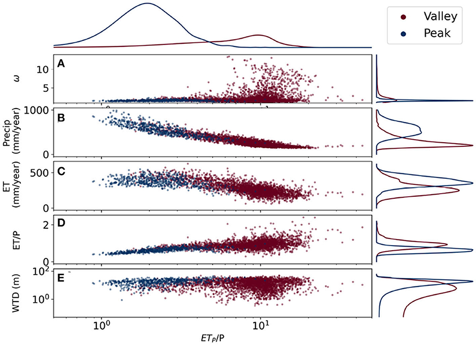
Figure 1. Relationship between aridity index (ET_P/P) and shape parameter ω (A), Precipitation (B), Evapotranspiration (ET; C), Evaporative index (ET/P; D), and water table depth (WTD; E). The blue dots represent for peak watersheds and the red dots represent for valley watersheds. (A) Some of the valley watersheds with the aridity index >8 have high (>3) ω; other valley and peak watersheds have relatively low ω with an average ω of 1.5. (B, C) The watersheds show linear relationships between precipitation and evapotranspiration to aridity index where the aridity index increases and the precipitation/evapotranspiration amount decreases. (D) While most of the precipitation in the peak watersheds contribute to runoff (evaporative index <0.8), in some valley watersheds, the precipitation amount is less than the evapotranspiration amount (evaporative index > 1.0). (E) Water table is generally deep (around 10 m) for peak watersheds and shallow for valley watersheds.

FIGURE 2

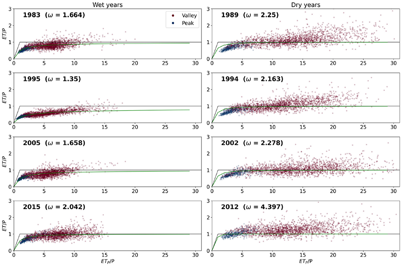
Figure 2. Budyko curves for selected dry and wet years. The blue dots represent for peak watersheds and the red dots represent for valley watersheds. The watersheds are plotted against evaporative index (ET/P) and aridity index (ET_P/P). Selected wet years are: 1983, 1995, 2005, and 2015. Selected dry years are: 1989, 1996, 2002, and 2012.

FIGURE 3

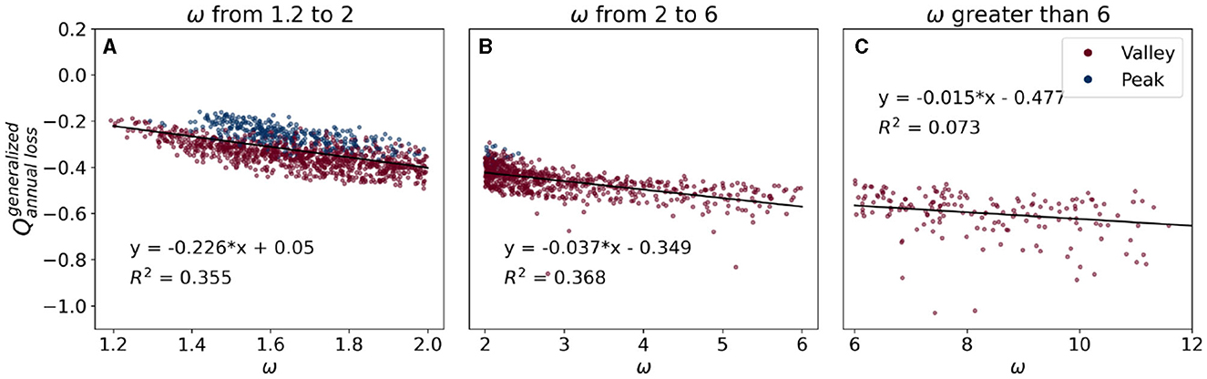
Figure 3. Generalized streamflow loss as a function of the shape parameter ω. Generalized streamflow loss is calculated as in Section 2.4. Blue dots denote the peak watersheds, red dots denote the valley watersheds. (A–C) Show average generalized streamflow loss in different ranges of shape parameter ω and their corresponding coefficient of determination (R²).

3.1. Two distinct types of watersheds within the UCRB

We find that the watershed delineation scheme is accurate in two distinct types of watersheds within the UCRB (Figure 1). Figures 1B, C display precipitation and ET as functions of aridity index and watershed types. Peak watersheds have a much higher precipitation rate of around 800 mm/year compared with around 275 mm/year from valley watersheds. ET also happens more in peak watersheds (>280 mm/year) than in valley watersheds (<280 mm/year). Figure 1D shows the Budyko scatter plot of the peak (blue dots) and valley (red dots) watersheds. This figure indicates precipitation in peak watersheds contributes to runoff or groundwater recharge (ET/P <0.5) and most precipitation in the valley watersheds becomes ET (ET/P closer or larger than 1). Lastly, water table for valley watersheds is shown to have higher variability than one for peak watersheds (Figure 1E).

Moreover, the shape parameter ω values are also drastically different for peak and valley watersheds (Figure 1A). While the shape parameters ω of peak watersheds are consistent across the UCRB with ω ranging from 1.2 to 1.5, ω of valley watersheds show much more variability with ω ranging from 1.2 to 10. Downstream valley watersheds, whose aridity indices are high (>5) and evaporative index are >1, have the most extreme values of shape parameters, with ranges between 5 and 10 (Figure 1A). With dry years will likely to happen more frequent in the future, we then focus on the behaviors of the peak and valley watersheds in selected “wet” and “dry” years in the next section.

3.2. New insight into wet and dry years

Figure 2 shows Budyko plots of the UCRB's watersheds for representative “wet” and “dry” years. The aridity index differentiates dry years from wet years. The aridity indices (ET_P/P) for wet years exhibit a range of 0.8–15, with median values of 2.31 for peak watersheds and 7.23 for valley watersheds. In contrast, during dry years, the aridity indices span from 0.8 to over 20, with median values of 3.12 for peak watersheds and 12.44 for valley watersheds. Peak watersheds show an average shift of 1.2 in aridity indices between wet and dry years. While the aridity indices increased for the whole UCRB in the dry years, precipitation in peak watersheds is still contributing to runoff and recharging processes with the evaporative index (ET/P) consistently smaller than 1 except for the water year (WY) 2012. The WY 2012 is an exceptional dry year which results to high evaporative index of peak watersheds and much higher evaporative index of valley watersheds (Figure 2). On the other hand, during dry years, the shift for aridity indices in valley watersheds is higher with an average shift of 3.5 and the maximum shift of 10 (Figure 2). The high evaporative index (ET/P > 1) of valley watersheds is reflected by their high shape parameters ω. In a same aridity condition, higher the shape parameter led to higher evaporative index. This led to the streamflow loss of the valley watersheds.

3.3. Relationship between streamflow loss and the shape parameter ω

Figure 3 shows the generalized streamflow loss in dry years as a function of the shape parameter ω. Shape parameters for peak watersheds only range from 1.2 to 2. With similar shape parameter range between 1.2 and 2, valley watersheds (red dots) experienced higher streamflow loss (average −0.35) than peak watersheds (blue dots; average −0.24) (Figure 3A). Streamflow losses increased when ω are increased up to 6 with average $Q_{annualloss}^{generalized}$ of −0.41 and −0.6 for ω in 2–6 and >6, respectively. The coefficient of determination (R²) between streamflow losses and ω for watersheds with ω smaller than 2 and with ω from 2 to 6 are 0.355 and 0.368, respectively. When ω are >6, there is no clear relationship between streamflow losses and ω (the corresponding R² is 0.073). One possible explanation of this no clear relationship is watersheds with high ω (ω > 6) have a wider range of WTD values (Figure 1). In watersheds that have high ω and low WTD (red dots that have ω from 6 to 10 in Figure 1A and WTD values closed to 0 in Figure 1E), their streamflow was subsidized by lateral groundwater flow (Figure 4). Thus, their generalized streamflow losses ($Q_{annualloss}^{generalized}$) are lower than ones from watersheds that have high ω and high WTD. To conclude, watersheds with small to medium shape parameters (ω from 1.2 to 6) show a strong relationship between theirs $Q_{annualloss}^{generalized}$and theirs corresponding ω.

FIGURE 4

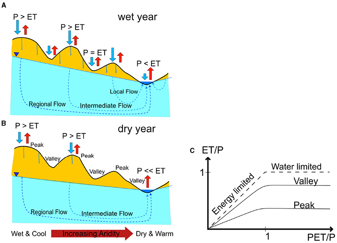
Figure 4. A conceptual diagram for peak and valley watersheds. (A, B) show the difference in precipitation and evapotranspiration for cross-sections of peak and valley watersheds during wet and dry years. For the wet year (A) the whole system gets recharged; precipitation is much higher than ET in peak watersheds; ET amount approaches the amount of precipitation and surpasses precipitation in discharge points. For the dry year (B) the system only gets recharged by precipitation in peak watersheds in which ET is much stronger than one in a wet year; the water table is lower than in the wet year; in discharge points, ET is much higher than precipitation which takes water out of the system. There is a transition in aridity where the peak watersheds are more wet and cool and the valley watersheds are more dry and warm. (C) Shows different Budyko curves for peak and valley watersheds. The peak watershed has lower omega value thus flatter curve than the valley watershed. Diagram modified and combined from several prior studies (Tóth, 1963; Haitjema and Mitchell-Bruker, 2005; Gleeson and Manning, 2008; Fan and Schaller, 2009; Maxwell et al., 2016; Carroll et al., 2019).

As mentioned in Section 2.4, the UCRB is comprised on multiple river systems such as the Green (northern UCRB), the Gunnison (eastern UCRB) or the San Juan (southeastern UCRB) (Supplementary Figure S1). Since each system has its own distinct aridity index (Yang et al., 2009; Knowles et al., 2015), we could find similar behaviors in Figure 3 if we examine each river system individually (i.e., study the relationship between ω and Q_annualloss for all sub-watersheds belong to the same river system). We would find that, in a single river system, the peak sub-watersheds have low ω and stable stream loss, while as the river travels further downstream, the valley sub-watersheds have higher ω and more volatile stream loss. A conceptual explanation for this behavior is illustrated in Figure 4 and discussed in the next section. Subtracting the $0.25^{*}\frac{ET}{P}$ term from Q_annualloss is not an ad-hoc formulation of the loss index. We did that only to shift all curves of the river systems into one and provide to readers a more generalize view of how peak and valley watersheds behave in the UCRB.

Lastly, there are a portion of valley watersheds that have low ω (ω <2) which are shown in Figures 1A, 3A. While peak watersheds have low ω in part because they have high precipitation (mean annual precipitation is >600 mm), those “low ω” valley watersheds have lowest ET in the basin (Figure 1C; Supplementary Figure S1B), moderate temperature of 278 K mean annual (Supplementary Figure S1C) and shallow WTD (Figure 1E). Most of those “low ω” valley watersheds locate in the Green River Basin (North of the UCRB) whose terrain is flat. River systems originated from the Green River Basin exhibit the same behavior of streamflow loss when ω in the river system increase from upstream to downstream.

4. Conclusion and discussion

Streamflow loss because of ET in the UCRB has been well-studied. However, due to the UCRB complex topography, which part of the basin losses more water during dry years remains an open question. In our study, we analyzed the heterogeneity of streamflow loss due to ET of sub-watersheds within the UCRB using Budyko curves.

We started by dividing UCRB sub-watersheds into either peak or valley watersheds based on their topographic characteristics (Supplementary Figure S2). Then, using a 37-year hydrological dataset (Tran et al., 2022), we calculated the hydrologic characteristic for each of the watersheds. Peak and valley watersheds are found to be distinctive in term of evaporative index, dryness index, precipitation and WTD (Figure 1). This distinctive behavior leads to different responses of peak and valley watersheds to evaporative water during dry years.

In dry years, valley watersheds experienced a much bigger shift in both the aridity index and evaporative index than the peak watersheds, 3.5–1.2 for aridity and 1.2–0.8 for evaporative indices, respectively. The big shift in Budyko curve leads to an overall higher shape parameter of the valley watershed (an average value of 3.1) than the peak watershed (an average value of 1.3). When comparing with the streamflow loss in dry years relatively to normal years, the shape parameter ranges from 1.2 to 2 and from 2 to 6 correlates well with R² of 0.355 and 0.368, respectively. The shape parameter can then be used to describe the severity of streamflow loss for a watershed during dry years.

Figure 4 shows our conceptual diagram of peak and valley watersheds dynamics during wet and dry years. Cross-sections of peak watersheds are represented by three “mountains” while ones of valley watersheds are represented by three “depressions” of the figure. During wet years, the groundwater gets recharged from the both the peak and valley regions on the right-hand side of the figure which leads to high water table and more groundwater lateral flows to streams (blue region—Figure 4A). During dry years, the groundwater gets recharged in much fewer places (in only two peaks) which leads to lower water table and fewer lateral flows to stream (Figure 4B). Figure 4C shows an example of how the Budyko curve might look like for peak and valley watersheds: peak watersheds have lower ω hence flatter Budyko curves while valley watersheds have higher ω so their corresponding Budyko curves are closer to the limit lines. The lateral flows during dry years are exacerbating water loss of the basin during warming since these flows subsidize ET in valley watersheds leading to more loss in total flow. Previous studies have shown the role of groundwater in adjusting the Budyko curve. Carroll et al. (2019) shown groundwater releases to streams more during dry years, resulting in a water table elevation decline. Condon and Maxwell (2017) shown that positive groundwater contribution can shift the Budyko curve vertically by contributing more to ET. In conjunction with other metrics used to predict streamflow anomalies, such as the snowmelt rate (Barnhart et al., 2016), the fraction of annual precipitation as snowfall (Berghuijs et al., 2014), and the Snow Storage Index (SSI; Hale et al., 2023), the descriptive behavior of ω to watershed's streamflow loss is an important finding which might be applied to other headwaters systems.

One limitation of this study is the use of a shorter timeframe for calculating the Budyko shape parameters compared to the typical 50-year study periods employed in previous research (Berghuijs et al., 2014; Barnhart et al., 2016; Hale et al., 2023). Given that dry and wet years can be relative to local climate conditions, a follow-up study could investigate the sensitivity of peak and valley watersheds to their respective local drought events. It is important to note that different approaches to the Budyko hypothesis such as “effective precipitation” (Chen et al., 2013; Condon and Maxwell, 2017) and “direct evapotranspiration” (this study; Condon and Maxwell, 2017) could yield different results of ω. Therefore, approach to the Budyko hypothesis should be highlighted along with the assessment of ω. The “direct evapotranspiration” approach is useful in many cases when the groundwater system is not directly measured.

Open research

The simulations were conducted using ParFlow version 3.6.0 (https://zenodo.org/record/4639761#.YovpAZPMLVs). The data processing step was done using Python3.7 programming language with necessary toolboxes including NumPy (https://numpy.org/), the Geospatial Data Abstraction Library (GDAL; https://gdal.org/) and the Python Data Analysis Library (PANDAS; https://pandas.pydata.org/).

The simulation dataset used for this study is hosted in CyVerse: https://doi.org/10.25739/nv2q-ct31. For more information related to the dataset, please referred to Tran et al. (2022).

Data availability statement

The datasets presented in this study can be found in online repositories. The names of the repository/repositories and accession number(s) can be found in the article/Supplementary material.

Author contributions

HT: Conceptualization, Data curation, Formal analysis, Investigation, Methodology, Validation, Visualization, Writing—original draft, Writing—review and editing. CY: Conceptualization, Investigation, Writing—review and editing. LC: Funding acquisition, Project administration, Resources, Supervision, Writing—review and editing. RM: Funding acquisition, Investigation, Project administration, Resources, Supervision, Writing—review and editing.

Funding

The author(s) declare financial support was received for the research, authorship, and/or publication of this article. High-performance computing for ParFlow-CLM simulations were provided by the National Center for Atmospheric Research Computational and Information Systems Laboratory. This work was supported by the US National Science CyberInfrastructure project, HydroFrame (NSF-OAC 1835903) and the IDEAS-Watersheds (DOE Office of Science) project.

Conflict of interest

The authors declare that the research was conducted in the absence of any commercial or financial relationships that could be construed as a potential conflict of interest.

Publisher's note

All claims expressed in this article are solely those of the authors and do not necessarily represent those of their affiliated organizations, or those of the publisher, the editors and the reviewers. Any product that may be evaluated in this article, or claim that may be made by its manufacturer, is not guaranteed or endorsed by the publisher.

Supplementary material

The Supplementary Material for this article can be found online at: https://www.frontiersin.org/articles/10.3389/frwa.2023.1258367/full#supplementary-material

References

Abatzoglou, J. T., and Ficklin, D. L. (2017). Climatic and physiographic controls of spatial variability in surface water balance over the contiguous United States using the Budyko relationship. Water Resour. Res. 53, 7630–7643. doi: 10.1002/2017WR020843

CrossRef Full Text | Google Scholar

Bai, P., Liu, X., Zhang, D., and Liu, C. (2020). Estimation of the Budyko model parameter for small basins in China. Hydrol. Process. 34, 125–138. doi: 10.1002/hyp.13577

CrossRef Full Text | Google Scholar

Barnett, T. P., and Pierce, D. W. (2008). When will Lake Mead go dry? Water Resour. Res. 44, 3201. doi: 10.1029/2007WR006704

CrossRef Full Text | Google Scholar

Barnett, T. P., and Pierce, D. W. (2009). Sustainable water deliveries from the Colorado River in a changing climate. Proc. Natl. Acad. Sci. U. S. A. 106, 7334–7338. doi: 10.1073/pnas.0812762106

PubMed Abstract | CrossRef Full Text | Google Scholar

Barnhart, T. B., Molotch, N. P., Livneh, B., Harpold, A. A., Knowles, J. F., and Schneider, D. (2016). Snowmelt rate dictates streamflow. Geophys. Res. Lett. 43, 8006–8016. doi: 10.1002/2016GL069690

CrossRef Full Text | Google Scholar

Barsugli, J. J., Ray, A. J., Livneh, B., Dewes, C. F., Heldmyer, A., Rangwala, I., et al. (2020). Projections of mountain snowpack loss for wolverine denning elevations in the Rocky Mountains. Earth's Future 8, e2020EF001537. doi: 10.1029/2020EF001537

CrossRef Full Text | Google Scholar

Berghuijs, W., Woods, R., and Hrachowitz, M. (2014). A precipitation shift from snow towards rain leads to a decrease in streamflow. Nat. Clim. Change 4, 583–586. doi: 10.1038/nclimate2246

CrossRef Full Text | Google Scholar

Budyko, M. (1963). Evaporation Under Natural Conditions. Israel Program for Scientific Translations. Available online at: https://agris.fao.org/agris-search/search.do?recordID=US201300573953

Google Scholar

Budyko, M. (1974). Climate and Life. Available online at: https://agris.fao.org/agris-search/search.do?recordID=US201300514816

Google Scholar

Carroll, R. W. H., Deems, J. S., Niswonger, R., Schumer, R., and Williams, K. H. (2019). The importance of interflow to groundwater recharge in a snowmelt-dominated headwater basin. Geophys. Res. Lett. 46, 5899–5908. doi: 10.1029/2019GL082447

CrossRef Full Text | Google Scholar

Chen, X., Alimohammadi, N., and Wang, D. (2013). Modeling interannual variability of seasonal evaporation and storage change based on the extended Budyko framework. Water Resour. Res. 49, 6067–6078. doi: 10.1002/wrcr.20493

CrossRef Full Text | Google Scholar

Christensen, N. S., and Lettenmaier, D. P. (2007). A multimodel ensemble approach to assessment of climate change impacts on the hydrology and water resources of the Colorado River Basin. Hydrol. Earth Syst. Sci. 11, 1417–1434. doi: 10.5194/hess-11-1417-2007

CrossRef Full Text | Google Scholar

Christensen, N. S., Wood, A. W., Voisin, N., Lettenmaier, D. P., and Palmer, R. N. (2004). The effects of climate change on the hydrology and water resources of the Colorado River basin. Climat. Change 62, 337–363. doi: 10.1023/B:CLIM.0000013684.13621.1f

CrossRef Full Text | Google Scholar

Colorado Department of Natural Resources (2021). Drought Condition Report for August 2021. Available online at: https://dnrweblink.state.co.us/cwcbsearch/0/edoc/215346/GovReportAug2021.pdf?searchid=f403b1f3-0f91-497e-aad2-c69539792cdd (accessed September 22, 2023).

Google Scholar

Condon, L. E., and Maxwell, R. M. (2017). Systematic shifts in Budyko relationships caused by groundwater storage changes. Hydrol. Earth Syst. Sci. 21, 1117–1135. doi: 10.5194/hess-21-1117-2017

CrossRef Full Text | Google Scholar

Cosgrove, B. A., Lohmann, D., Mitchell, K. E., Houser, P. R., Wood, E. F., Schaake, J. C., et al. (2003). Real-time and retrospective forcing in the North American Land Data Assimilation System (NLDAS) project. J. Geophys. Res. 108, 8842. doi: 10.1029/2002JD003118

CrossRef Full Text | Google Scholar

Donohue, R. J., Roderick, M. L., and McVicar, T. R. (2007). On the importance of including vegetation dynamics in Budyko's hydrological model. Hydrol. Earth Syst. Sci. 11, 983–995. doi: 10.5194/hess-11-983-2007

CrossRef Full Text | Google Scholar

Fan, Y., and Schaller, M. F. (2009). River basins as groundwater exporters and importers: Implications for water cycle and climate modeling. J. Geophys. Res. Atmosph. 114, 4103. doi: 10.1029/2008JD010636

CrossRef Full Text | Google Scholar

Feng, X., Porporato, A., and Rodriguez-Iturbe, I. (2015). Stochastic soil water balance under seasonal climates. Proc. R. Soc. A Math. Phys. Eng. Sci. 471, 20140623. doi: 10.1098/rspa.2014.0623

PubMed Abstract | CrossRef Full Text | Google Scholar

Feng, X., Vico, G., and Porporato, A. (2012). On the effects of seasonality on soil water balance and plant growth. Water Resour. Res. 48, W05543. doi: 10.1029/2011WR011263

CrossRef Full Text | Google Scholar

Foster, L. M., Bearup, L. A., Molotch, N. P., Brooks, P. D., and Maxwell, R. M. (2016). Energy budget increases reduce mean streamflow more than snow-rain transitions: using integrated modeling to isolate climate change impacts on Rocky Mountain hydrology. Environ. Res. Lett. 11, 044015. doi: 10.1088/1748-9326/11/4/044015

CrossRef Full Text | Google Scholar

Fu, B. (1981). On the calculation of evaporation from land surface in mountainous areas (in Chinese). Sci. Atmos. Sin. 5, 23–31.

Google Scholar

Gentine, P., D'Odorico, P., Lintner, B. R., Sivandran, G., and Salvucci, G. (2012). Interdependence of climate, soil, and vegetation as constrained by the Budyko curve. Geophys. Res. Lett. 39, L19404. doi: 10.1029/2012GL053492

CrossRef Full Text | Google Scholar

Gleeson, T., and Manning, A. H. (2008). Regional groundwater flow in mountainous terrain: three-dimensional simulations of topographic and hydrogeologic controls. Water Resour. Res. 44, 10403. doi: 10.1029/2008WR006848

CrossRef Full Text | Google Scholar

Haitjema, H. M., and Mitchell-Bruker, S. (2005). Are water tables a subdued replica of the topography? Ground Water 43, 781–786. doi: 10.1111/j.1745-6584.2005.00090.x

PubMed Abstract | CrossRef Full Text | Google Scholar

Hale, K. E., Musselman, K. N., Newman, A. J., Livneh, B., and Molotch, N. P. (2023). Effects of snow water storage on hydrologic partitioning across the mountainous, western United States. Water Resour. Res. 59, e2023WR034690. doi: 10.1029/2023WR034690

CrossRef Full Text | Google Scholar

Hamel, P., and Guswa, A. J. (2015). Uncertainty analysis of a spatially explicit annual water-balance model: case study of the Cape Fear basin, North Carolina. Hydrol. Earth Syst. Sci. 19, 839–853. doi: 10.5194/hess-19-839-2015

CrossRef Full Text | Google Scholar

Harding, B. L., Wood, A. W., and Prairie, J. R. (2012). The implications of climate change scenario selection for future streamflow projection in the Upper Colorado River Basin. Hydrol. Earth Syst. Sci. 16, 3989–4007. doi: 10.5194/hess-16-3989-2012

CrossRef Full Text | Google Scholar

Immerzeel, W. W., van Beek, L. P. H., and Bierkens, M. F. P. (2010). Climate change will affect the asian water towers. Science 328, 1382–1385. doi: 10.1126/science.1183188

PubMed Abstract | CrossRef Full Text | Google Scholar

Knowles, J. F., Harpold, A. A., Cowie, R., Zeliff, M., Barnard, H. R., Burns, S. P., et al. (2015). The relative contributions of alpine and subalpine ecosystems to the water balance of a mountainous, headwater catchment. Hydrol. Process. 29, 4794–4808. doi: 10.1002/hyp.10526

CrossRef Full Text | Google Scholar

Li, D., Pan, M., Cong, Z., Zhang, L., and Wood, E. (2013). Vegetation control on water and energy balance within the Budyko framework. Water Resour. Res. 49, 969–976. doi: 10.1002/wrcr.20107

CrossRef Full Text | Google Scholar

Mastrotheodoros, T., Pappas, C., Molnar, P., Burlando, P., Manoli, G., Parajka, J., et al. (2020). More green and less blue water in the Alps during warmer summers. Nat. Clim. Change 10, 155–161. doi: 10.1038/s41558-019-0676-5

CrossRef Full Text | Google Scholar

Maxwell, R. M., and Condon, L. E. (2016). Connections between groundwater flow and transpiration partitioning. Science 353, 377–380. doi: 10.1126/science.aaf7891

PubMed Abstract | CrossRef Full Text | Google Scholar

Maxwell, R. M., Condon, L. E., Kollet, S. J., Maher, K., Haggerty, R., and Forrester, M. M. (2016). The imprint of climate and geology on the residence times of groundwater. Geophys. Res. Lett. 43, 701–708. doi: 10.1002/2015GL066916

CrossRef Full Text | Google Scholar

Miller, M. P., Buto, S. G., Susong, D. D., and Rumsey, C. A. (2016). The importance of base flow in sustaining surface water flow in the Upper Colorado River Basin. Water Resour. Res. 52, 3547–3562. doi: 10.1002/2015WR017963

CrossRef Full Text | Google Scholar

Milly, P. C. D. (1993). An analytic solution of the stochastic storage problem applicable to soil water. Water Resour. Res. 29, 3755–3758. doi: 10.1029/93WR01934

CrossRef Full Text | Google Scholar

Milly, P. C. D. (1994). Climate, soil water storage, and the average annual water balance. Water Resour. Res. 30, 2143–2156. doi: 10.1029/94WR00586

CrossRef Full Text | Google Scholar

Milly, P. C. D., and Dunne, K. A. (2020). Colorado River flow dwindles as warming-driven loss of reflective snow energizes evaporation. Science 367, 1252–1255. doi: 10.1126/science.aay9187

PubMed Abstract | CrossRef Full Text | Google Scholar

Mitchell, K. E., Lohmann, D., Houser, P. R., Wood, E. F., Schaake, J. C., Robock, A., et al. (2004). The multi-institution North American Land Data Assimilation System (NLDAS): Utilizing multiple GCIP products and partners in a continental distributed hydrological modeling system. J. Geophys. Res. Atmosp. 109, D07S90. doi: 10.1029/2003JD003823

CrossRef Full Text | Google Scholar

Natural Resources and Conservation Service (2021). Colorado Water Availability Task Force. Denver, CO: Colorado Water Conservation Board.

Google Scholar

Porporato, A., Daly, E., and Rodriguez-Iturbe, I. (2004). Soil water balance and ecosystem response to climate change. Am. Nat. 164, 625–632. doi: 10.1086/424970

PubMed Abstract | CrossRef Full Text | Google Scholar

Rumsey, C. A., Miller, M. P., Susong, D. D., Tillman, F. D., and Anning, D. W. (2015). Regional scale estimates of baseflow and factors influencing baseflow in the Upper Colorado River Basin. J. Hydrol. Reg. Stud. 4, 91–107. doi: 10.1016/j.ejrh.2015.04.008

CrossRef Full Text | Google Scholar

Ryken, A. C., Gochis, D., and Maxwell, R. M. (2022). Unravelling groundwater contributions to evapotranspiration and constraining water fluxes in a high-elevation catchment. Hydrol. Process. 36, e14449. doi: 10.1002/hyp.14449

CrossRef Full Text | Google Scholar

Tóth, J. (1963). A theoretical analysis of groundwater flow in small drainage basins. J. Geophys. Res. 68, 4795–4812. doi: 10.1029/JZ068i016p04795

CrossRef Full Text | Google Scholar

Tran, H., Zhang, J., Cohard, J. M., Condon, L. E., and Maxwell, R. M. (2020). Simulating groundwater-streamflow connections in the upper Colorado River Basin. Groundwater 58, 392–405. doi: 10.1111/gwat.13000

PubMed Abstract | CrossRef Full Text | Google Scholar

Tran, H., Zhang, J., O'Neill, M. M., Ryken, A., Condon, L. E., and Maxwell, R. M. (2022). A hydrological simulation dataset of the Upper Colorado River Basin from 1983 to 2019. Sci. Data 9, 1–17. doi: 10.1038/s41597-022-01123-w

PubMed Abstract | CrossRef Full Text | Google Scholar

U.S. Department of the Interior Bureau of Reclamation (2012). Annual Operating Plan for Colorado River Reservoirs 2013. Available online at: https://www.usbr.gov/uc/water/rsvrs/ops/aop/AOP11_final.pdf (accessed September 22, 2023).

Google Scholar

Udall, B., and Overpeck, J. (2017). The twenty-first century Colorado River hot drought and implications for the future. Water Resour. Res. 53, 2404–2418. doi: 10.1002/2016WR019638

CrossRef Full Text | Google Scholar

Woodhouse, C. A., Smith, R. M., McAfee, S. A., Pederson, G. T., McCabe, G. J., Miller, W. P., et al. (2021). Upper Colorado River Basin 20th century droughts under 21st century warming: Plausible scenarios for the future. Clim. Serv. 21, 100206. doi: 10.1016/j.cliser.2020.100206

CrossRef Full Text | Google Scholar

Xiao, M., Udall, B., and Lettenmaier, D. P. (2018). On the causes of declining colorado river streamflows. Water Resour. Res. 54, 6739–6756. doi: 10.1029/2018WR023153

PubMed Abstract | CrossRef Full Text | Google Scholar

Xu, X., Liu, W., Scanlon, B. R., Zhang, L., and Pan, M. (2013). Local and global factors controlling water-energy balances within the Budyko framework. Geophys. Res. Lett. 40, 6123–6129. doi: 10.1002/2013GL058324

CrossRef Full Text | Google Scholar

Yang, D., Shao, W., Yeh, P. J. F., Yang, H., Kanae, S., and Oki, T. (2009). Impact of vegetation coverage on regional water balance in the nonhumid regions of China. Water Resour. Res. 45, W00A14. doi: 10.1029/2008WR006948

CrossRef Full Text | Google Scholar

Yang, D., Sun, F., Liu, Z., Cong, Z., Ni, G., and Lei, Z. (2007). Analyzing spatial and temporal variability of annual water-energy balance in nonhumid regions of China using the Budyko hypothesis. Water Resour. Res. 43, W04426. doi: 10.1029/2006WR005224

CrossRef Full Text | Google Scholar

Yang, H., Qi, J., Xu, X., Yang, D., and Lv, H. (2014). The regional variation in climate elasticity and climate contribution to runoff across China. J. Hydrol. 517, 607–616. doi: 10.1016/j.jhydrol.2014.05.062

PubMed Abstract | CrossRef Full Text | Google Scholar

Yao, L., and Wang, D. (2022). Hydrological basis of different budyko equations: the spatial variability of available water for evaporation. Water Resour. Res. 58, e2021WR030921. doi: 10.1029/2021WR030921

CrossRef Full Text | Google Scholar

Zhang, L., Dawes, W. R., and Walker, G. R. (2001). Response of mean annual evapotranspiration to vegetation changes at catchment scale. Water Resour. Res. 37, 701–708. doi: 10.1029/2000WR900325

CrossRef Full Text | Google Scholar

Zhang, L., Hickel, K., Dawes, W. R., Chiew, F. H. S., Western, A. W., and Briggs, P. R. (2004). A rational function approach for estimating mean annual evapotranspiration. Water Resour. Res. 40, W02502. doi: 10.1029/2003WR002710

CrossRef Full Text | Google Scholar