 Colin A. Richardson*
 R. Edward Beighley
- Department of Civil and Environmental Engineering, Northeastern University, Boston, MA, United States
Surface water flooding represents a significant hazard for many infrastructure systems. For example, residential, commercial, and industrial properties, water and wastewater treatment facilities, private drinking water wells, stormwater systems, or transportation networks are often impacted (i.e., in terms of damage or functionality) by flooding events. For large scale events, knowing where to prioritize recovery resources can be challenging. To help communities throughout North Carolina manage flood disaster responses, near real-time state-wide rapid flood mapping methods are needed. In this study, Height Above Nearest Drainage (HAND) concepts are combined with National Water Model river discharges to enable rapid flood mapping throughout North Carolina. The modeling system is calibrated using USGS stage-discharge relationships and FEMA 100-year flood maps. The calibration process ultimately provides spatially distributed channel roughness values to best match the available datasets. Results show that the flood mapping system, when calibrated, provides reasonable estimates of both river stage (or corresponding water surface elevations) and surface water extents. Comparing HAND to FEMA hazard maps both in Wake County and state-wide shows an agreement of 80.1% and 76.3%, respectively. For the non-agreement locations, flood extents tend to be overestimated as compared to underestimated, which is preferred in the context of identifying potentially impacted infrastructure systems. Future research will focus on developing transfer relationships to estimate channel roughness values for locations that lack the data needed for calibration.
1 Introduction
Throughout the US and globally, flood disasters are one of the worst natural disasters in terms of loss of life and damage (Jonkman, 2005; Wing et al., 2020). Climate change and urbanization are likely to further exacerbate the impacts of flooding (Shao et al., 2020; Rashid et al., 2023). For assessing locations that have potential to flood, flood hazard maps published as part of the Federal Emergency Management Agency (FEMA) National Flood Insurance Program are generally available. These maps are useful indicators of flood risk throughout the United States (US) as they provide the expected flood boundaries of the 1% annual exceedance probability (AEP) (i.e., 100-year return period) events, and are based on well-established hydrologic and hydraulic modeling frameworks such as the Hydrologic Engineering Center's River Analysis System (HEC-RAS) developed by the US Army Corps of Engineers (USACE, 2016). While these maps provide a general flood hazard assessment across the US, they require detailed input data (e.g., LIDAR or cross-sectional surveys and river discharge/stage observations) and do not provide hazard information for specific flooding events. For event specific flood mapping, efforts using remote sensing techniques such as those used by the Dartmouth Flood Observatory (Brakenridge, 2023) and showcased in numerous studies (Syifa et al., 2019; DeVries et al., 2020; Shahabi et al., 2020; Kalantar et al., 2021; Tripathi et al., 2021; Ammirati et al., 2022). These mapping efforts make use of a variety of earth observation data products from sources including Landsat 8, Sentinel 1, and MODIS, and through change detection algorithms they allow for the creation of event specific flood maps and continuous monitoring. However, cloud cover, data latency, and spatial-temporal resolution impacts can be significant challenges to these methods in terms of providing near-real-time flood maps.
In cases where near-real-time or forecasted flood mapping is needed for mitigation and recovery efforts, hydrodynamic models can be used. Many hydrodynamic models have been employed for flood mapping such as 1 and 2 dimensional HEC-RAS models (Farooq et al., 2019; Salman et al., 2021; Tamiru and Dinka, 2021; Namara et al., 2022; Vashist and Singh, 2023), LISFLOOD-FP (Amarnath et al., 2015; Rahimzadeh et al., 2019; Rajib et al., 2020; Nandi and Reddy, 2022), and FLO-2D (Haltas et al., 2016; Erena et al., 2018; Cruz et al., 2019; Li et al., 2021) to name a few. These models are commonly used in practice and provide the basis for some of the flood risk information sources mentioned above. Due to the large amount of input data and time required to develop, run, and validate these types of models, as well as the significant computational requirements, they generally lend themselves to smaller scale and more detailed modeling efforts. Leveraging recent advances in large scale model systems such as NASA's North American Land Data Assimilation System (NLDAS) and the US National Weather Service's National Water Model (NWM), a suite of applications have been developed to allow for near real-time and short-term forecasts across the US (Xia et al., 2012; Kumar et al., 2017; Abdelkader et al., 2023). These platforms are both powerful and valuable due to their extents covering the entirety of the US, and their abilities to provide information on the current and future hydrologic conditions. These platforms do not, however, include flood mapping and must be coupled to some sort of flood mapping method to provide more actionable information related to flood extents.
In contrast to hydrodynamic models, geomorphic modeling methods relating basin geomorphology to floodplain extents using morphometric relationships have been widely developed and applied in the past for floodplain delineation (Noman et al., 2001; Gallant and Dowling, 2003; Dodov and Foufoula-Georgiou, 2006; Nardi et al., 2006; Manfreda et al., 2011; Degiorgis et al., 2012; Jalayer et al., 2014; Samela et al., 2016). These methods leverage the landscape shaping effect of floods and terrain analysis to generate simplified relationships for floodplain identification based on a basin's morphology. By combining simplified hydrologic methods for estimating flood depths with geomorphic terrain analyses, hydrogeomorphic methods are born which can be used for floodplain delineation in areas where hydrologic observations (e.g., stage, discharge, etc.) are scarce. Multiple hydrogeomorphic methods have been developed under this paradigm including the GFPLAIN algorithm (Nardi et al., 2006, 2018, 2019), and the Geomorphic Flood Index (GFI) (Manfreda et al., 2015; Samela et al., 2016, 2017). Both GFPLAIN and GFI inform the varying flood depth used for floodplain delineation using a contributing drainage area scaling relationship based on the work of Leopold and Maddock (1953), but GFPLAIN flags floodplain cells as those with elevations less than the maximum flood elevation, while GFI classifies floodplain cells by comparing the natural logarithm of the ratio between the maximum flood depth and the height above the nearest hydrologically connected river cell to a specific threshold value for binary classification. One geomorphic method used for mapping flood extents from large scale models such as the NWM is Height Above Nearest Drainage (HAND) (Afshari et al., 2018; Garousi-Nejad et al., 2019; Johnson et al., 2019; Aristizabal et al., 2023). HAND is a geomorphic method that takes a digital elevation model (DEM) as an input and converts the elevation data into a relative elevation wherein every cell represents the local height above the nearest hydrologically connected drainage channel (Rennó et al., 2008; Nobre et al., 2011). In 2018, CyberGIS computation schemes have allowed for the generation of HAND data products across the Conterminous US (Liu et al., 2018). Additionally, coupling reach-averaged channel geometries extracted from DEM's, Manning's Equation for open channel flow, and an assumed Manning's roughness value allows for the generation of synthetic rating curves (SRCs) at the reach scale where a given discharge can be converted to depth of water for a particular reach (Zheng et al., 2018). Herein lies the rapid aspect of the HAND method compared to conventional hydraulic models, since the only required input to generate a flood map is a discharge, which can be converted to a water depth using a SRC and subtracted from the preprocessed HAND layer to create an inundation map for an area of interest. Recently, HAND has been coupled with the NWM to allow for near-real-time and forecasted flood mapping across the Conterminous US (Johnson et al., 2019). While the work in Johnson et al. (2019) found that the HAND + NWM method contained some issues with flood extent prediction in lower order reaches and areas of low relief, the researchers did find that HAND + NWM was generally able to distinguish between areas of lower and higher flood risk, especially in higher order reaches. It should be noted that the SRCs generated in Zheng et al. (2018) and used in Johnson et al. (2019) were created using a uniform Manning's roughness value of 0.05, and the researchers note that the performance of the HAND + NWM method could likely be improved if the SRCs were calibrated using the Manning's roughness parameter.
In this study, the HAND methodology is used to enable rapid, state-wide flood mapping. Central to this study is the calibration of the SRC relationships for all catchments within NC. Calibration includes three different approaches for three geographic domains, with the first entailing the calibration of SRC relationships to best match rating curve field measurements obtained at United States Geological Service (USGS) gauges throughout Wake County, NC. For the second, SRC relationships are calibrated to maximize agreement with FEMA hazard maps in Wake County using 1% AEP discharges extracted from the HEC-RAS models used to create the FEMA maps. Finally, SRC relationships are calibrated to maximize agreements with FEMA hazard maps across all of NC using 1% AEP discharges generated using USGS regional regression equations.
2 Methods
2.1 Study area and data sources
The study region for this analysis is shown in Figure 1. All data included in this study were obtained from publicly available data sources. The preprocessed HAND, National Hydrography Dataset Medium Resolution (NHDPlus MR) catchment files, NHDPlus MR flow line files, and SRC tables covering the extent of NC were obtained from version 0.2.1 of the Continental Flood Inundation Mapping Data Repository for HAND and Hydraulic Property Tables maintained by Oak Ridge National Laboratory (Liu et al., 2020). Version 0.2.1 utilizes a stream etching process which improves HAND performance at the intersections of streams and roads where the original DEM may not accurately represent the flow path of the stream. These data are provided on the USGS HUC6 unit basis. All HUC6 unit boundaries within or crossing the state boundary were used to obtain the required input data. The HAND layers, NHDPlus MR catchments, NHDPlus MR flowlines, and SRC table files were merged respectively to produce seamless data layers for the analysis. These data preprocessing steps were accomplished through the use of QGIS 3.28 for raster and vector data, and the Pandas Python package for the SRC tables. Ultimately, a total of 69,071 NHDPlus MR catchments were included in the statewide analysis, with a subset of 1,995 catchments included in the Wake County analysis.
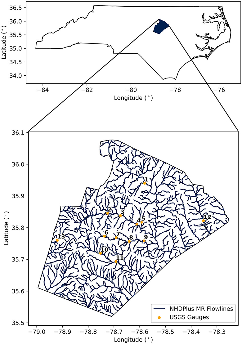
Figure 1. Top: study region extent (North Carolina) with Wake County shown in blue; Bottom: magnified view of Wake County with NHDPlus MR flowlines shown in blue and USGS gauge locations shown as points labeled according to the Site IDs in Table 1.
The USGS gauges within Wake County (Figure 1) that possessed stage and discharge field measurements necessary to generate site specific rating curves were identified using the USGS Site Web Service (USGS, 2023). Only active gauge sites within Wake County, NC with recently updated field measurements and upstream drainage areas >10 km2 were considered for this analysis, which resulted in 13 total sites being included. The USGS gauges included in this study are listed in Table 1.
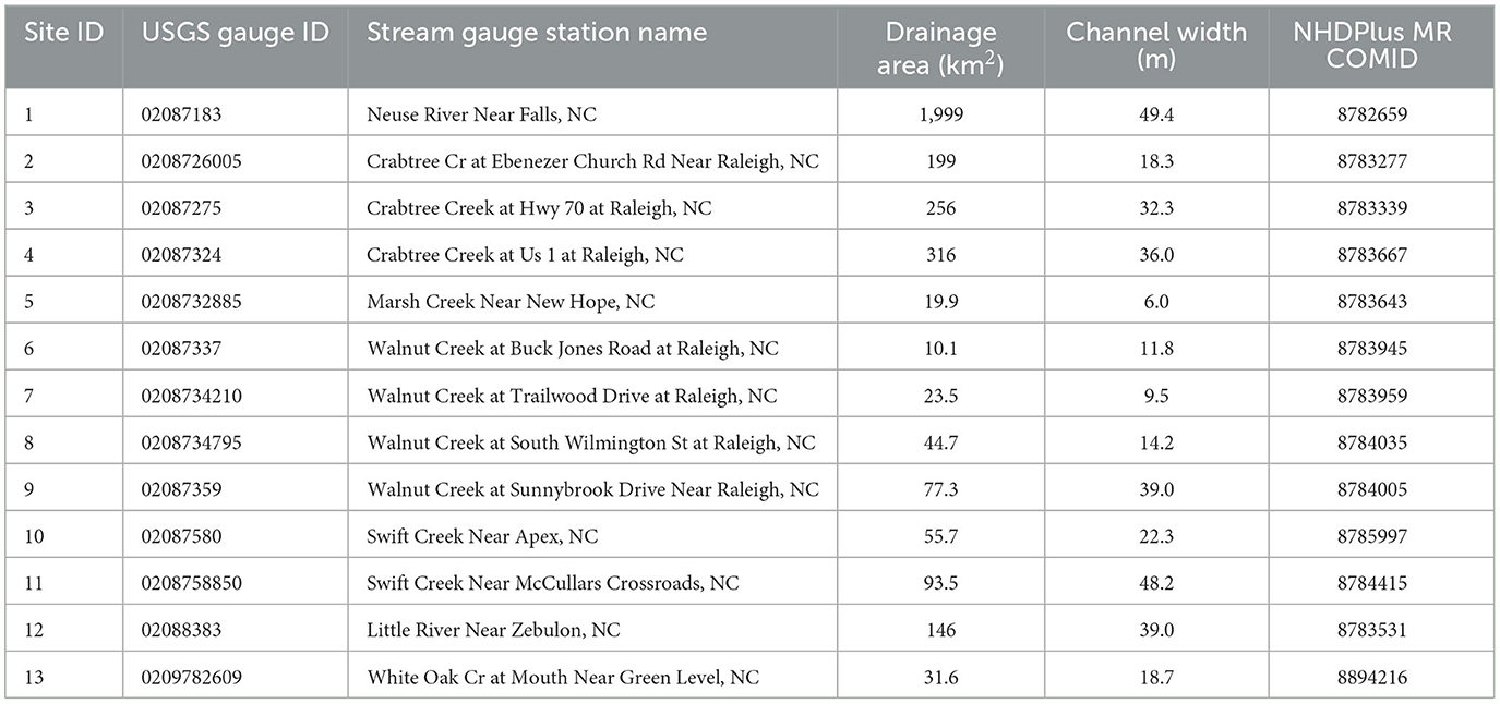
Table 1. A list of all USGS gauges included in this study with the gauge ID, station name, total upstream drainage area (km2), channel width (m) corresponding to the maximum discharge available from the USGS field measurements, and the NHDPlus MR common identifier (COMID) corresponding to each USGS gauge shown in Figure 1.
FEMA hazard maps and related metadata were obtained from the FEMA Map Service Center (FEMA, 2023). Specifically, the geodatabase encompassing all of the effective FEMA National Flood Hazard Layer for NC was acquired, and the statewide flood hazard boundary for the 1% AEP event as well as the discharge nodes representing 1% AEP flow change locations within Wake County, NC were utilized within this study. Ultimately, 1,566 discharge nodes were available which fell within 707 of the 1,995 NHDPlus MR catchments present in Wake County. Additionally, FEMA hazard maps were only available in 49,230 of the 69,071 NHDPlus MR catchments present in NC. Accordingly, only catchments with FEMA hazard maps and discharges available within their bounds were able to be calibrated, and for catchments that possessed multiple FEMA discharges, a catchment average discharge was calculated and used in the calibration process. The FEMA 1% AEP hazard map and the discharge nodes within Wake County are shown in Figure 2.
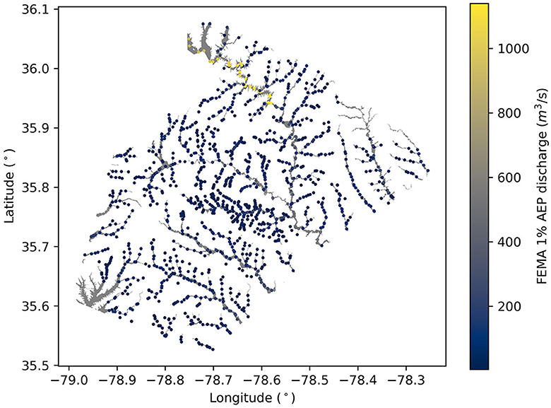
Figure 2. FEMA 1% AEP hazard boundary for Wake County with FEMA 1% AEP discharge nodes.
Impervious surface land cover data were obtained from the National Land Cover Dataset (NLCD) for the year of 2021 (Dewitz, 2023). These data were available throughout the entire study area at a 30 × 30m resolution and represented the percentage of impervious area in each pixel. By classifying catchments according to their level of impervious cover, the calibration performance in urban vs. rural catchments was compared.
2.2 Calibration approach
This section describes the general calibration process and the metrics used to evaluate the final performance of the calibration. Central to the calibration process is the development of continuous rating curves, which are used in all three portions of the calibration approach. The calibration approach is broken into three separate analyses: rating curves for gauge locations within Wake County, flood boundaries with known discharges for Wake County, and state-wide flood boundaries with discharges estimated from regional relationships.
2.2.1 Rating curve functions
To allow for direct comparison between USGS and SRC derived stage-discharge data, continuous rating curves (RCs) were developed using the USGS field measurements and all NHDPlus MR reaches included in the analysis. These RCs take the form of Equation 1, where H represents water stage in m, Q represents reach discharge in m3/s, and a and b are coefficients specific to each USGS gauge or NHDPlus MR reach.
Use of continuous RCs also promotes the operational goal of rapid flood mapping across NC by eliminating the need for interpolation within the original USGS and SRC tabular data, which imparts a significant computational load. For the SRC derived RCs, the underlying stage-discharge data are originally calculated using Manning's Equation for open channel flow (Equation 2) where Q is discharge in m3/s, n is the Manning's Roughness coefficient, A is the cross-sectional area of flow in m2, R is the hydraulic radius in m, and S is the channel slope in m/m.
Because Equation 2 underlays the SRC derived RCs, the only parameter available to calibrate these relationships is the Manning's n coefficient as the other quantities in Equation 2 are derived from the HAND layers (i.e., A and R) or the flowlines (i.e., S) pertaining to each NHDPlus MR reach. Consequently, during the SRC RC calibration process, only the a coefficient is adjusted as the b coefficient remains the same for each reach no matter how the Manning's n value is adjusted.
Once calibration for a reach has been completed, the a coefficient for the RC for a given reach is adjusted using a scale factor c. The c value is calculated using Equation 3 where n-2 is the calibrated Manning's Roughness coefficient, n–1 is the original uniform Manning's Roughness coefficient of 0.05, and b is the RC coefficient specific to each NHDPlus MR reach.
The calibrated RC incorporating the scale factor c takes the form of Equation 4, where H' is the adjusted reach stage in m, Q is the reach discharge in m3/s, a and b are the original RC coefficients, c is the scale factor given by Equation 3, and a' is the calibrated leading coefficient.
As a precursor to the calibration process, RCs were generated for each USGS gauge and for each NHDPlus MR reach included in the study area. For this study, the fifty most recent field measurements available at each gauge listed in Table 1 were utilized to generate the USGS RCs. This step ensures that the RCs were generated using the most relevant field measurement data to the present while also possessing a sufficient number of measurements to extract a general rating curve relationship. Of the 50 most recent measurements, any measurements with a quality rating of “Poor” as determined by the USGS technicians were discarded. Additionally, because the SRC stage values are referenced to the HAND cells equal to zero for a certain reach, and the USGS field measurements are referenced to their respective gauge datum, a standardization of the two sets of stages was required. This was accomplished by determining the minimum DEM elevation where HAND was also equal to zero in the vicinity of the gauge location, and subtracting this elevation from the USGS water surface elevation values for that gauge location to create adjusted USGS stage values which are congruent with the definition of the SRC stages. In this process, any negative adjusted stage values are discarded before the generation of the USGS RCs. For the SRC RCs, the entire set of stage-discharge points available for each NHDPlus MR reach were utilized to generate the RCs. The function curve_fit() from the Python package SciPy was utilized to determine the appropriate values for a and b from Equation 1 for each USGS and SRC RC using the default function parameters (Virtanen et al., 2020). To assess the goodness-of-fit for both the USGS and SRC RCs, the R2 value between the original USGS or SRC points and the respective RC was calculated.
2.2.2 USGS gauge calibration
With RCs developed for each USGS gauge and NHDPlus MR reach, the NHDPlus MR catchments corresponding to each gauge location were determined by intersecting the gauge point locations with the NHDPlus MR catchment polygons. The intersected NHDPlus MR catchments provided the COMIDs associated with each intersected catchment which allowed for the corresponding SRC RC to be associated with each USGS RC. Additionally, the upstream drainage areas associated with the USGS gauges and the intersected NHDPlus MR catchments were compared and checked to match to ensure the USGS field measurements and SRC data were referring to the same drainage basins.
For each pair of associated USGS and SRC RCs, the SRC RC was adjusted to best match the USGS RC by holding the SRC RC b coefficient value constant while employing the curve_fit() function again to determine the optimal adjusted a coefficient value (i.e., a' in Equation 4) that minimized the residual error when compared against the stage values produced by the USGS RC. Figure 3 represents the general process described herein for USGS Gauge #02087183, Neuse River Near Falls, NC, where the general intent is to determine the optimal a coefficient for the SRC RC that results in the closest match to the USGS RC.
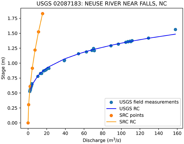
Figure 3. Calibration example for USGS gauge #02087183, Neuse River Near Falls, NC.
To assess the goodness-of-fit, the relative root mean square error (rRMSE) between the USGS RC and the calibrated SRC RC were calculated according to Equation 5 where HSRCi is the stage generated by the SRC RC for each discharge included in the USGS field measurements for a site in m, HUSGSi is the stage generated by the USGS RC for each discharge included in the USGS field measurements for a site in m, is the mean of the USGS stage values for a site, and n is the total number of stage values compared between the SRC RC and USGS RC.
2.2.3 Wake county FEMA calibration
The calibration process for Wake County uses the FEMA discharge nodes, NHDPlus MR reaches, and FEMA hazard maps shown in Figure 2. The FEMA 1% AEP discharge value for each NHDPlus MR reach was determined by spatially joining the nodes to the NHDPlus MR catchments polygons. For catchments in which more than one node existed, the average discharge value was assigned to that catchment. Using the uncalibrated RC associated with each NHDPlus MR reach, the initial water stage in meters was calculated using the FEMA discharge value assigned to said reach. A HAND flood map was created for each initial stage value by determining which cells in the HAND layer for a particular reach were less than or equal to the initial stage value. Next, the associated FEMA hazard maps for Wake County were clipped to the equivalent extent of the created HAND flood maps.
To maximize the spatial agreement between HAND produced flood maps and FEMA hazard maps depicting the same map extent, all cells in the two maps being compared were categorized as wet-wet (WW) for cells inundated in both maps, wet-dry (WD) for cells inundated in the HAND map but not inundated in the FEMA hazard map, dry-wet (DW) for cells inundated in the FEMA hazard map but not inundated in the HAND map, and dry-dry (DD) for cells shown as not inundated in both the HAND map and the FEMA hazard map. Using the relative counts of cells in each of these four categories, agreement between the HAND map and the FEMA hazard map is calculated using Equation 6.
The portion of the comparison where the HAND map overpredicts inundation compared to the FEMA hazard map is calculated using Equation 7.
Finally, the portion of the comparison where the HAND map underpredicts inundation compared to the FEMA hazard map is calculated using Equation 8.
These AOU metrics have been adapted from Johnson et al. (2019) to allow for comparison between the two flood maps. Note that the three AOU statistics sum to 100% indicating the relative proportions of agreement, overprediction, and underprediction in the flood mapping extent being analyzed. The initial AOU statistics (i.e., before calibration) were calculated for each reach according to Equations 6–8. These initial AOU values were saved for each reach to allow for comparison with the final AOU values to determine the improved agreement between the HAND and FEMA hazard maps following calibration.
For the actual calibration, the minimum and maximum HAND values present in a HAND layer corresponding to a particular reach were determined and a sequence of stage values incremented by 0.025 meters was generated between the minimum and the maximum values. For each stage in this sequence, a HAND flood map was generated, then AOU values between the HAND map and the FEMA hazard map were calculated, and the corresponding stage and AOU values were cataloged for each reach. The maximum HAND vs. FEMA agreement was determined from the cataloged stage and AOU values, and the corresponding optimal stage value for each reach was determined to be the stage associated with the maximum agreement for each reach.
Using the initial and optimal stage values, the calibrated Manning's n value was determined using Equation 9, where n2 is the calibrated Manning's Roughness coefficient, A2 is the cross-sectional flow area from the SRC table associated with the optimal stage (H' in Equation 4) in m2, R2 is the hydraulic radius from the SRC table associated with the optimal stage in m, A1 is the cross-sectional flow area from the SRC table associated with the initial stage in m2, R1 is the hydraulic radius from the SRC table associated with the initial stage in m, and n1 is the original uniform Manning's Roughness of 0.05.
Lastly, the SRC RC scale factor was calculated using Equation 3 and the updated SRC RC was created using Equation 4 in which the original a coefficient value was multiplied by the scale factor c value so that the optimal stage value H' is generated when the FEMA 1% AEP discharge is input to the calibrated SRC RC. For reaches in which no FEMA discharge nodes were available, the calibration was not performed to ensure only flood maps derived from known discharges were compared. Figure 4 shows an example HAND vs. FEMA flood map comparison for NHDPlus MR reach 8783261, where the general intent of the calibration scheme is to maximize the areas where both flood maps agree by adjusting the stage generated by the SRC RC.
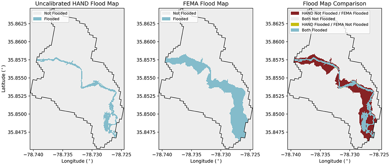
Figure 4. Example HAND vs. FEMA flood map comparison used in calibration for NHDPlus MR reach 8783261.
2.2.4 North Carolina FEMA calibration
The statewide FEMA calibration scheme was nearly identical to the Wake County calibration scheme described in Section 2.2.3, with the only difference being the method for determining the 1% AEP discharge associated with each NHDPlus MR reach. Due to the FEMA discharge nodes not being available for all NHDPlus MR reaches in which a FEMA hazard map was published, 1% AEP discharge values were estimated using USGS regional regression equations for the State of NC (Feaster et al., 2023). To determine the 1% AEP discharges, Equation 10 [from Table 2 in Feaster et al. (2023)] was used where Q1% is the 1% AEP discharge in m3/s; PCT1, PCT2, PCT3, and PCT5 are the drainage area percentages falling within hydrologic regions 1, 2, 3, and 5 in % from Feaster et al. (2023), and DA is the total upstream drainage area in square miles.
2.3 Urban vs. rural calibration comparison
As identified in Di Baldassarre et al. (2020) a common drawback of hydrogeomorphic flood mapping methods, like those employed in this study, is that they cannot account for the role of hydraulic structures and other artificial alterations on the determination of the floodplain extents in a basin. To examine the effect of this drawback, the calibration results were classified into urban and rural categories using NLCD imperviousness data (Dewitz, 2023). First, the percentage of impervious cover in each catchment was calculated using the Zonal Statistics tool in QGIS 3.28, and a threshold of 20% impervious cover was selected based on the low end of the developed land classification from the full NLCD dataset. Catchments with >20% impervious cover were classified as urban and catchments below 20% impervious cover were classified as rural. Using this breakdown of urban and rural catchments, the relative calibration performance was examined to evaluate the effect of artificial catchment modifications on the efficacy of the calibration.
3 Results and discussion
3.1 USGS gauge calibration results
The results of initially fitting the USGS and uncalibrated SRC RCs as described in Section 2.2.1, and adjusting the SRC RC a coefficient as described in Section 2.2.2, are shown in Table 2, where the values for the number of USGS field measurements used to fit the USGS RC, the USGS a and b coefficients, the R2 value of the USGS RC, the uncalibrated SRC a and b coefficients, the R2 value of the uncalibrated SRC RC, the calibrated SRC -a' coefficient (i.e., c * a in Equation 4), and rRMSE for the calibrated SRC RC are shown. Generally, the USGS RCs fit the field measurements well with USGS R2 values at or above 0.9, though sites 6 and 13 yield lower values of 0.74 and 0.56, respectively. In contrast, the SRC R2 values are all very near 1 indicating close adherence of the SRC RCs to the original SRC points. Note that the SRC RCs were expected to fit the relationship well given they were derived from Manning's Equation and reach-averaged quantities that were developed by systematically increasing stage values (i.e., HAND values).
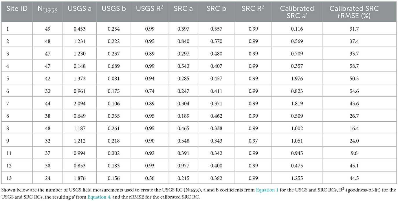
Table 2. RC generation results for USGS, uncalibrated SRC, and calibrated SRC RCs according to the Site ID shown in Table 1.
The overall results of the USGS gauge calibration scheme are shown in Figure 5, where the USGS field measurements, original SRC points, USGS RC, uncalibrated SRC RC, and the calibrated SRC RC are all shown for each for each site listed in Table 1. The resulting mean RMSE value is 0.41 m, ranging from 0.085 m to 0.80 m (Figure 5). While RMSE has units of meters, the stages across the 13 sites are roughly the same order of magnitude. Thus, rRMSE, RMSE normalized by the range in stages used for the calibration (Table 2), is used for comparisons. The median rRMSE is 37% ranging from 10% to 59%. A key finding is that rRMSE tends to increase as channel width decreases (Table 1). This is likely due to resolution issues as the reach-averaged HAND values are based on 10 m resolution DEM values as compared to the survey-based cross-sectional data used at the gauge locations.
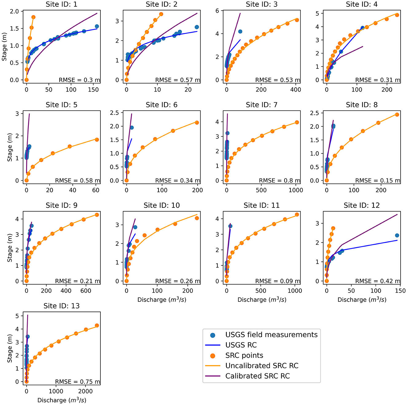
Figure 5. USGS calibration results with each plot Site ID corresponding to the gauges listed in Table 1. The vertical axes show water stage in meters, with the horizontal axes showing discharge in m3/s. The RMSE between the SRC RC and the USGS RC is shown in the bottom right corner of each plot.
The scale factors and calibrated Manning's roughness coefficients (n2) associated with each USGS gauge site are shown in Table 3. In summary, the USGS calibration results in a mean scale factor of 2.75 ranging from 0.29 to 6.93. In terms of roughness values, the mean value is 1.38 ranging from 0.0054 to 6.22 across all sites. The wide range of scale factor and corresponding n2 values suggest that the SRC RCs calibrated under this method require significantly different adjustments depending on the gauge location, highlighting the potential mismatch between high-resolution cross-sectional vs. coarser resolution reach-averaged quantities. Ideally, the scale factor would be close to one with variations leading to more reasonable increases/decreases in roughness from the baseline value of 0.05. Here, 10 of 13 sites have resulting roughness values between 0.01 and 1.0. Given the scaling between cross-sectional vs. reach-averaged hydraulic characteristics, the resulting range in effective roughness seems reasonable at those 10 sites. The high values at the remaining 3 sites need further investigation (e.g., limited range in H-Q pairs, unique hydraulic controls at the gauge locations, uncertainty in the DEM data along the reach, etc.) Two of the three sites (5 and 7) with high n2 values have widths <10 m (Table 1). The remaining site (13) with a high n2 value only had an R2 value of 0.56 for the USGS RC suggesting the H-Q relationship is not well defined at this location. Additional challenges include the range of USGS field measurement pairs used to conduct the calibration. For example, the USGS RC for site 13 was generated for a relatively small range in stage (1.5–3.2 m) and discharge (0.02–11.7 m3/s) and only achieved an R2 value of 0.56. For sites like this, an expansion of the field measurements used to generate the USGS RC may be beneficial to the calibration process to include a wider range of stage-discharge pairs in the subset of field measurements. While no definitive relationship was found between available gauge site characteristics (e.g., reach averaged slope or width) and calibrated roughness, the above rationale suggests that with additional research it may be possible to develop transfer functions to estimate roughness values for ungauged locations.

Table 3. Scale factors and calibrated Manning's roughness coefficients (n2) across all USGS gauge sites according to the three calibration methods explained in Sections 2.2.2–2.2.4.
In general, calibration for each USGS gauge site resulted in SRC RCs adhering much closer to the USGS field measurements as compared to the uncalibrated SRC RCs. However, it is clear that error is generally present in the lower and upper ranges of discharge values for each set of USGS field measurements. This error persists due to the unchanging b coefficient between the uncalibrated and calibrated SRC RCs, which remains constant because Manning's Equation (Equation 2) is used to create the SRC RC approximations. Because the constant b coefficient effectively dictates the shape of the RC, there is a built-in limitation to the calibration process which prevents the SRC RC from more closely matching the USGS RC unless their two b coefficients happen to be similar.
Since the USGS field measurements are collected in-situ and more accurately reflect the localized hydraulic controls dictating the stage-discharge relationship at a gauge, and the SRC relationships are approximated from 10 m resolution DEMs using an empirical formula (Equation 2), it is not surprising that there would be some level of inherent incongruency between the SRC and USGS RCs. In the context of this work supporting rapid flood mapping, it must be determined whether or not this inherent incongruency truly matters when attempting to project impacted areas before, during, or after flooding events. With the USGS gauge calibration focused on matching SRC RCs to the USGS stages (i.e., water surface elevation measurements if the gauge datum is applied), it is crucial to evaluate these calibrated relationships in contrast to the flooding extent-based calibrations encompassed in the Wake County and Statewide FEMA calibration results discussed next.
3.2 Wake County FEMA calibration results
Figure 6 shows the final agreement between the calibrated HAND and FEMA flood maps generated from the Wake County calibration. First, we look at AOU statistics aggregated over all 707 of the 1995 NHDPlus MR catchments in the Wake County study area. The AOU statistics given by Equations 6–8 resulted in an initial agreement of 62.4%, an initial underprediction of 24.8%, and an initial overprediction of 12.8%. The final calibration resulted in a final agreement of 80.1%, a final underprediction of 5.4%, and a final overprediction of 14.5%. These values indicate a 28.4% increase in agreement (17.7 percentage points improvement), a 78.2% decrease in underprediction (19.4 percentage points), and a 13.3% increase in overprediction (1.7 percentage points). Overall, this calibration significantly improved the agreement between the HAND and FEMA flood maps, supporting the cause of improving the prediction of flood extents for large events like the 1% AEP flood. Additionally, the decrease in underprediction and increase in overprediction appears preferrable in the operational context of this work related to rapid flood hazard mapping. This is because a moderate overprediction can be translated to a larger population designated as at risk of flooding, while a moderate underprediction can be translated to a smaller population designated as at risk of flooding. To a certain extent, overprediction is preferred since underprediction could result in some populations not being notified of flood risk when they potentially should be. In addition, locations overpredicted are likely near the actual flood boundary and only separated by a modest elevation gradient. Thus, there is still potential for flood water to enter wells via shallow subsurface flow paths.
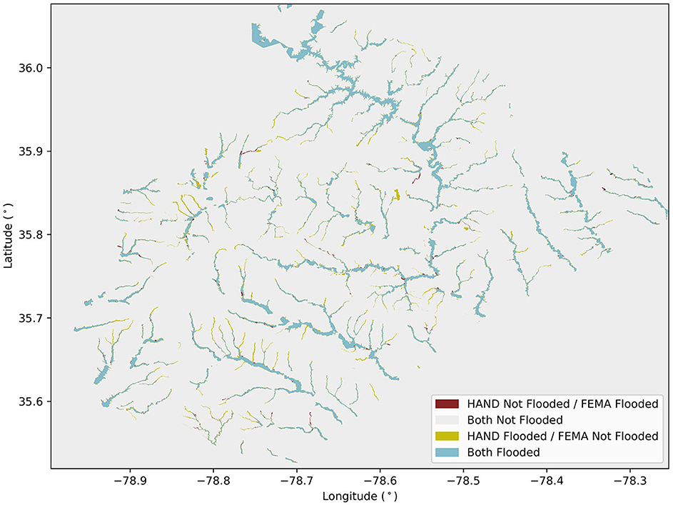
Figure 6. Final HAND vs. FEMA agreement for the 707 NHDPlus MR catchments included in the Wake County calibration.
Looking at the HAND vs. FEMA agreement at the catchment scale, the initial catchment average agreement was 57.2%, while the final catchment average agreement is 72.7%, resulting in a 27.1% improvement (15.5 percentage points) in agreement following calibration. Additionally, the standard deviation of the optimal agreement throughout all catchments was 25.0%, while the minimum, median, and maximum agreement values were 0.17%, 81.8%, and 100%, respectively. This wide range of agreement values indicates that the FEMA hazard map extent-based calibration approach varies in efficacy from catchment to catchment, with some catchments able to match FEMA bounds nearly identically and others not coming close. Judging by the final catchment average agreement and the overall Wake County calibrated agreement, it is clear that the majority of catchments possess good calibration results, though the calibrated SRC RCs associated with very low catchment agreement must be further examined. In some instances, the FEMA hazard map and the HAND map did not cover the same extent of a catchment, with the FEMA map generally covering a smaller portion of the catchment extent. This is likely due to where the creators of the FEMA map decided to delineate their study area in lower order reaches, thus resulting in a somewhat uneven comparison between the HAND and FEMA maps in these reaches. In summary, these edge cases will be further investigated in future work, with alternative methods of determining the optimal scale factor for these cases being a focus.
The spatial distribution of SRC scale factors for all NHDPlus MR catchments included in the Wake County calibration is shown in Figure 7 with areas of white indicating catchments that were not calibrated as part of this analysis. Additionally, the specific scale factors for the NHDPlus MR catchments associated with the USGS gauges are shown in Table 3, though three catchments associated with USGS sites 1, 3, and 13 did not possess FEMA 1% AEP discharges. Thus, no scale factors were determined for these catchments. Of the 707 catchments for which scale factors were determined, 24% have values within the range of 0.75–1.25 (i.e., minimal scaling) and 40% have values within the range of 0.25–0.75 or 1.25–1.75 (i.e., moderate scaling). However, there does not appear to be any spatial pattern in the scale factors. By examining the correlation of catchment scale factors with different catchment characteristics (i.e., drainage area, soil type, average HAND value, land use, etc.), it may be possible to develop regional relationships that can determine SRC RC scale factors in catchments where no calibration could occur. This would allow for a seamless collection of SRC RCs to be generated across Wake County or all of NC, which could allow for gapless forecasted flood maps when coupling HAND and the NWM. This would also be particularly useful in the context of the Wake County calibration since less than half of the NHDPlus MR catchments included in Wake County were able to be calibrated using this method.
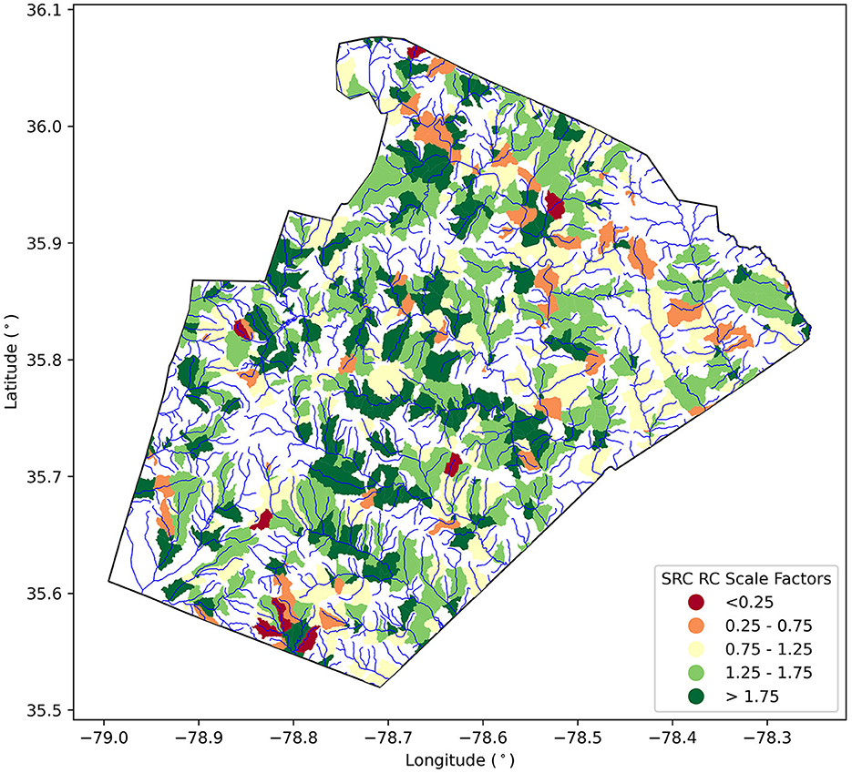
Figure 7. Scale factors for all catchments included in the Wake County calibration with the NHDPlus MR flowlines shown in blue.
Since a lack of FEMA 1% AEP discharges was the main reason for excluding so many catchments from this calibration scheme, it is possible that discharge interpolation based on the flow network provided with the NHDPlus MR dataset could fill in the data for catchments missing discharges. Though this method would still not allow for determination of a RC scale factor for catchments in which a FEMA hazard map has not been published.
3.3 North Carolina FEMA calibration results
Figure 8 shows the final agreement between the calibrated HAND and FEMA flood maps generated from the statewide calibration. For the statewide study area encompassing 49,230 of the 69,071 NHDPlus MR catchments, the AOU statistics given by Equations 6–8 resulted in an initial agreement of 47.2%, an initial underprediction of 38.9%, and an initial overprediction of 13.9%. The final calibration resulted in a final agreement of 76.3%, a final underprediction of 5.4%, and a final overprediction of 18.3%. These values indicate an overall 61.7% increase in agreement (29.1 percentage points), an 86.1% decrease in underprediction (33.5 percentage points), and a 31.7% increase in overprediction (4.4 percentage points), generally following the trend set by the Wake County calibration results. The lower initial agreement and higher initial underprediction from the statewide calibration compared to the Wake County calibration suggest that the 1% AEP discharges generated using the regional regression equations from Feaster et al. (2023) are underestimated compared to the FEMA 1% AEP discharges used in the Wake County calibration. It would make sense for the FEMA discharges to be more accurate since they are generated from hydrologic models (i.e., HEC-HMS) or more localized regression equations specific to the area encompassed in the FEMA hazard map. However, since the final agreement in the statewide calibration is comparable to the final agreement in the Wake County calibration, it appears that the calibration process was able to account for the differences in the source of the 1% AEP discharges. The discrepancy between the two sources of 1% AEP discharges will need to be examined to understand the effect of using these discharges on the RC scale factors generated, and on the operational forecasting of flood extents.
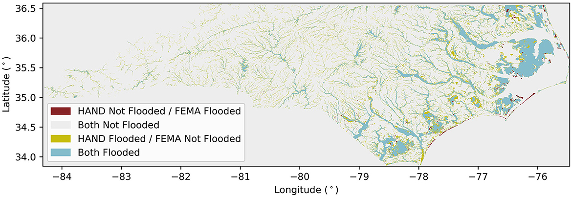
Figure 8. Comparison between FEMA and calibrated HAND flood maps for all 49,230 NHDPlus MR reaches included in the statewide calibration of North Carolina.
The distribution of the HAND vs. FEMA agreement and the optimal scale factor across all NHDPlus MR catchments included in the statewide calibration is shown in Figure 9. However, note that only the bottom 95% of the optimal scale factor data is shown in Figure 9 as a few extreme outlier scale factors prevented the distribution from being legible otherwise. Additionally, the specific scale factors and calibrated Manning's roughness coefficients (n2) for the NHDPlus MR catchments associated with the USGS gauge sites are shown in Table 3.
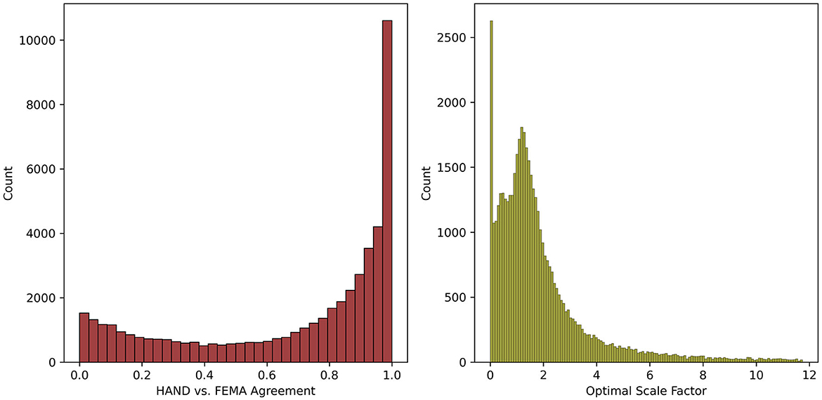
Figure 9. Histograms showing the distribution of the HAND vs. FEMA agreement and the optimal scale factors for the catchments included in the statewide calibration. The optimal scale factor histogram only includes the bottom 95% of scale factor data as extreme outliers in the top 5% (e.g., a scale factor of 6,823) prevented the plot from being legible.
Looking to the HAND vs. FEMA agreement distribution, 58.6% of catchments included in the statewide calibration show an agreement ≥0.75, with the remaining catchments possessing agreements <0.75 spread in a mostly uniform distribution. Building off the scale factor regionalization concept discussed in Section 3.2, it may be useful to build regionalization relationships using this subset of catchments which possess higher agreement. This could allow for higher quality scale factors to be developed for catchments which did not result in high agreement values in this current calibration scheme. The optimal scale factor distribution appears to be skewed to the left with a long and tapering tail to the right side. This tail represents increasingly large and rare scale factors ranging all the way to a maximum scale factor of 6,823 (not shown for legibility). These exceedingly high scale factors are another indication that the statewide calibration process seems to work well in many catchments, but in others the efficacy of the calibration is called into question. Additionally, the large number of catchments with scale factors close to or equal to 0 indicate scenarios where the calibration scheme is essentially attempting to turn flooding off for these catchments. This is similar to the Wake County calibration results where the FEMA map does not cover as much of the catchment as the HAND map. Thus, the resulting scale factors are excessively low as result of this process. For example, Figure 10 shows results for one catchment (scale factor = 0) where the FEMA flood map is only defined for a small portion of the catchment. In this case, the optimal stage is zero as this provides the maximum HAND vs. FEMA agreement, and the resulting scale factor prevents any river stage from being produced given the 1% AEP discharge input.
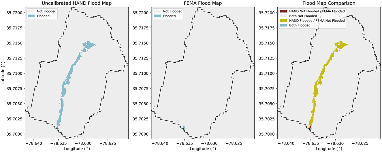
Figure 10. Flood mapping results for NHDPlus MR reach 8784365 showing a non-continuous FEMA flood map along a river.
3.4 Comparing calibration results
Scale factors and calibrated Manning's roughness coefficients (n2) associated with each USGS gauge site and across all three calibration schemes are shown in Table 3. When interpreting the scale factors it is helpful to note that values less than one indicate SRC RCs need to decrease the magnitude of stage required for a given discharge, while scale factors greater than one indicate SRC RCs need to increase the magnitude of stage required for a given discharge. A similar relationship is present for the n2 values where roughness values >0.05 indicate that the stage magnitude should be increased for a given catchment, and it should be decreased for roughness values <0.05. When the three scale factors associated with a particular USGS site are all either greater than or less than one, this indicates that the three methods generally agree in how the SRC RC should be modified. However, varying scale factors of greater than or less than one between calibration methods at a given site indicate that the methods disagree in how the SRC RC should be modified. Taking site 2 as an example, all three scale factors are less than one and all three n2 values are <0.05 indicating that the three calibration methods concur in how this particular SRC RC should be adjusted. Additionally, all three scale factors are rather close together when compared to the rest of the values in Table 3. Overall, this provides good confidence that the adjustment of the SRC RC associated with site 2 should result in lower stages at a given discharge as compared to the original uncalibrated RC. In contrast to site 2, site 4 possesses a scale factor <1 from the USGS calibration but has scale factors greater than one for the Wake County and Statewide calibrations. This discrepancy may be related to the fact that the USGS field measurements' maximum discharge for this site is 125 m3/s, while the 1% AEP discharges for the Wake County and statewide calibrations were 308 and 373 m3/s, respectively. Since the magnitude of discharges is quite different between the calibration methods, it is possible that the reach may have quite different stage responses to these large discharges, thus resulting in the varied scale factors based on the different calibration methods.
Comparing the n2 values between the Wake County and statewide calibration results in Table 3 clearly shows that there is some discrepancy amongst these values. Since the only difference between these two calibration schemes is the method for generating the input discharge, these discrepancies are closely linked to the differences in the 1% AEP discharges employed in each calibration. Figure 11 shows the relationship between the ratio of the Statewide and Wake County 1% AEP discharges (QState/QWake), and the ratio of the Statewide and Wake County calibrated n2 values (nState/nWake). Strikingly, nearly all sites where the QState/QWake value is <1 correspond to a nState/nWake value >1, while the inverse is true for QState/QWake values >1. This makes sense since a QState value < a QWake value would result in a proportionally higher nState value compared to the nWake value because a lower discharge at the same optimal stage would force a higher Manning's roughness value to meet that optimal stage. However, there are outliers in Figure 11 in which this relationship does not seem to hold. For example, the point in which the nState/nWake value is equal to 1, but the QState/QWake value is nearly equal to 4. This and other outliers occur due to discontinuities present in the underlying SRC tabular data used to generate the SRC RCs. The SRC tabular data are determined for a maximum stage value of roughly 25 m, and the initial stages generated by the uncalibrated SRC RCs are capped to this maximum value in order to keep the RC output within the stage range originally calculated for each SRC table. In the case of this example, both the Q-State and QWake discharges resulted in initial stage values above the maximum stage of 25 m, thus both were reduced to the maximum value. Thus, the initial stages and the corresponding optimal stages were equal for both calibration methods. Since the initial and optimal stage values were equal for each method, the final n2 value was also equal due to Equation 9. This type of discrepancy appears to only occur in catchments with SRC RCs that are particularly sensitive to the discharge input, resulting in stages above the 25 m limit. Other noise in the points shown in Figure 11 also appears to arise from the RC approximations used as a substitute to the raw SRC tabular data. While the RCs are very close approximations of the underlying SRC tables, they are still approximations introducing minor sources of error to the calibration process. Combining this minor error with the differences in the discharge inputs to both calibration schemes results in the slight shifts from the expected relationship between the ratios observed in Figure 11. Overall, there do appear to be edge cases where the efficacy of the SRC RC calibration is questionable, but the vast majority of cases show that the calibration scheme works as intended. In terms of future work, these edge cases will be addressed alongside catchments with low optimal agreement values and catchments with extreme scale factors in the development of a regionalization scheme for scale factors based on the catchment characteristics.
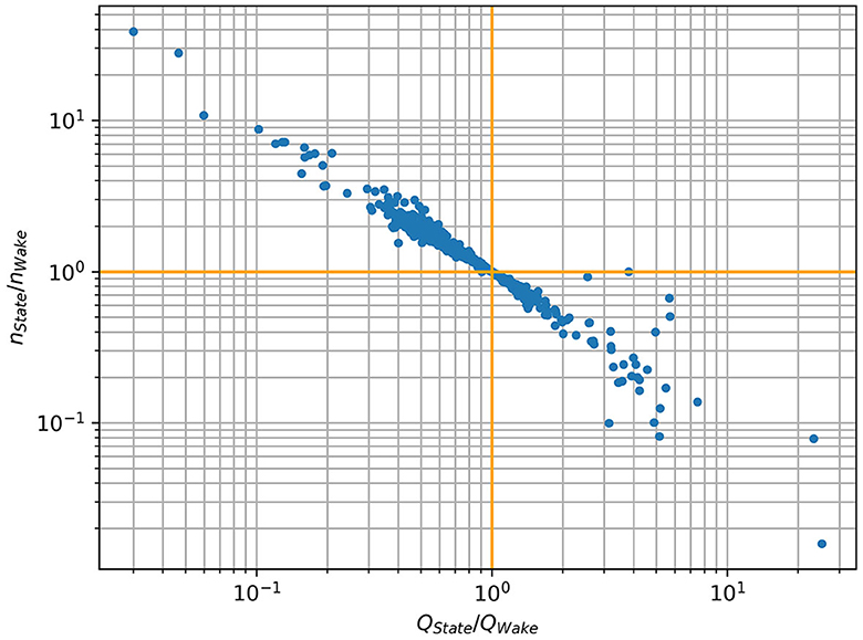
Figure 11. The ratio of the 1% AEP discharges between the Statewide calibration and the Wake County calibration (QState/QWake) vs. the ratio of the calibrated Manning's roughness coefficient between the statewide calibration and the Wake County calibration (nState/nWake).
3.5 Urban vs. rural calibration results
For the Wake County calibration, 210 of 707 catchments were classified as urban. Within this breakdown, urban catchments possessed an average optimal agreement of 63.0%, compared to 76.8% in catchments designated as rural indicating an overall better calibration performance in rural vs. urban catchments. The mean calibrated Manning's n value in urban catchments is 0.45 compared to 0.28 in rural catchments indicating a tendency for urban catchments to produce higher stages in general due to the heightened roughness coefficient. These results taken together illustrate a limitation of this calibration approach in urban catchments where the effects of hydraulic control structures and other human influence on the waterways are more pronounced. Since HAND coupled to a SRC is a hydrogeomorphic method, it cannot account for the effect of hydraulic control structures, so the effect of this infrastructure on the FEMA flood extents is bundled into the Manning's n coefficient during the HAND calibration.
For the Statewide calibration, 2,082 of 49,230 catchments were classified as urban. As discussed in Section 3.3, some catchments in the Statewide calibration resulted in extremely high scale factors and calibrated Manning's n values. These outlier values appear to result from combining the USGS estimated discharge inputs with poorly fit RC functions that overcorrect the calibrated Manning's n value and resulting scale factor. These outliers do not reflect efficacious calibration results, and will be addressed in future work, but for the sake of the current urban vs. rural comparison their effect is negated by only examining the bottom 90% of the Statewide output based on the scale factor of catchments. Using this subset, the urban catchments possessed an average optimal agreement of 62.5% compared to 68.3% in rural catchments. The mean calibrated Manning's n value in urban catchments is 0.35 compared to 0.28 in rural catchments. Similar to the Wake County results, these results reinforce the limitation of this calibration approach, and hydrogeomorphic methods in general, when applied in urban catchments.
By identifying this limitation in urban catchments, future work will focus calibration on non-urban catchments in order to minimize the effect of flood control infrastructure on the final calibration results. However, one upside for using hydrogeomorphic methods identified in Di Baldassarre et al. (2020) is that these methods can identify floodplains as if no flood protection were in place, thus producing more conservative estimates of flood plain extent. Taking this with the tendency of both the Wake County and Statewide calibrations to overpredict flooded area compared to the FEMA extents, we would rather more conservative flood bounds be generated when estimating the potential impacted population. This equates to a larger number of individuals designated as impacted which is preferable to underprediction and potentially missing impacted individuals.
Building off recent findings (Di Baldassarre et al., 2020; Lindersson et al., 2021), hydrogeomorphic methods can be valuable for the estimation of flood-prone areas, especially in data scarce regions, though, where available, they should be used in concert with more data intensive hydrologic flood mapping methods to better inform flood-prone area estimation. In the context of this research, hydrogeomorphic methods are intended to serve as a rapid and approximate estimation of flood hazards to people and infrastructure, though where data availability allows, these estimations will be supplemented and compared with hydrologic and remotely sensed flood extents to further inform the flood hazard estimation.
3.6 Limitations
The analysis and results presented in this study are not without limitations. The statewide calibration scheme relies upon estimated discharge inputs derived from regional regression equations (Equation 10). Since these equations are based solely on geographic region and basin drainage area, their use allows for a potential mismatch between the 1% AEP discharge and FEMA flood extent utilized in this calibration scheme, unlike in the Wake County calibration where flood extents were directly tied to the discharge inputs used for calibration. While this potential mismatch could reduce the efficacy of some catchment calibrations, the strength of the regional relationship lies in its ability to provide discharge inputs throughout the entirety of NC. One method of addressing this limitation could be further reliance on FEMA published 1% AEP discharge nodes available in other areas of NC. While the published nodes do not cover the entirety of NC, future work could also leverage data from the Flood Risk Information System (FRIS) published by the North Carolina Department of Public Safety (NCDPS, 2023). The FRIS provides engineering models used to generate FEMA hazard maps throughout NC, so further discharge nodes across NC could be extracted from these models, thus increasing the scope of catchments in which the 1% AEP discharge is directly associated with the FEMA hazard boundary being calibrated to.
The use of Manning's equation for steady open channel flow (Equation 2) to estimate flood stage is certainly an approximation of dynamic hydraulic processes and represents another limitation for a few reasons. Defining flood depth as a single uniform value per reach often serves as a good approximation, though this assumption may breakdown in longer reaches with greater elevation change from the high to low points. Assigning a single Manning's n value to each reach also introduces uncertainty since the roughness profile of the floodplain may vary depending on the magnitude and extent of the flood. Manning's equation is unable to account for unsteady flows and their varied flood stage effects. These limitations could be mitigated through the use of a compound uniform flow equation to differentiate between in-bank and overbank flows, by varying the Manning's n value throughout the reach, or by employing a more complex flow equation to account for unsteady flow effects. However, in concurrence with Zheng et al. (2018), the current use of Manning's equation is sufficient for approximate inundation mapping intended to screen flood risk rapidly at large scales.
Related to the use of Manning's equation to calculate flood depth, the original SRC data were calculated in a stage range of 0–25 meters. Following calibration and when using the 1% AEP discharge as an input, some RCs can produce stage values above the maximum value of 25 meters. Specifically, 11 of the 707 Wake County catchments and 395 of the 49,230 Statewide catchments produce this behavior, so in these cases the flood stage is limited to the 25-meter maximum value so as to not leave the range originally defined by the SRC tabular data. This limitation could be addressed by extending the range of stages included in the SRC tables to encompass more of the range of HAND values present in each catchment.
The number, extent, and data record of USGS gauges is also limited in this study. The gauges employed in this analysis were kept to those within Wake County as an initial venture into using these data for SRC RC parameter calibration, and to provide a means to compare water surface elevation-based RC calibration with the extent-based calibration employed in the rest of the study. After examining the performance of the USGS calibration, the limited degree to which the SRC RC could be modified to better match the USGS RC, and the limited number of active USGS field measurement stations we realized this method would not be suitable for wide calibration application unlike the extent-based calibration. Use of historical annual peak flow and stage measurements, which are generally more available, could serve as an alternative to the field measurement data used herein. This would also shift this calibration scheme to be more focused on higher return period events, which would be beneficial for mapping extents of larger and more destructive flood events.
Another limitation of this study is the geographic area in which it is currently applicable. Data availability varies across the various inputs to this analysis. The FEMA hazard boundaries and preprocessed HAND products (HAND layer, catchment layer, SRC tables, etc.) are available throughout the entirety of the conterminous US, though the 1% AEP discharge nodes are only partially available throughout the US where they have been published by FEMA. These data sources limit the current analysis to the bounds of the US, though other data sources could be employed to conduct a similar analysis elsewhere in the world. For terrain and hydrography, preprocessed global products like MERIT-Hydro (Yamazaki et al., 2019) or FABDEM (Hawker et al., 2022) could be used anywhere outside of the US with the HAND layer and SRC tables able to be generated from the underlying elevation data. Discharge inputs may not be available in-situ throughout much of the world, but remotely sensed discharge estimation techniques could be employed to provide discharges in data scarce regions (Brocca et al., 2020; Huang et al., 2020; Tarpanelli et al., 2023). The Surface Water Ocean Topography (SWOT) satellite launched in 2022 will also provide discharge estimates along with measurements of water surface extent for large rivers at a global scale, which could respectively serve as powerful inputs and calibration data in this optimization scheme (Revel et al., 2021; Durand et al., 2023). Additionally, crowdsourced or citizen science produced data could serve as other sources of information used to inform both discharge inputs and flood extents during real events (Le Coz et al., 2016; Weeser et al., 2019). Ultimately, the HAND optimization and rapid flood mapping scheme presented herein is flexible in that it could be applied elsewhere in the world provided data are available for the terrain, hydrography, discharge, and water surface extent inputs to this method.
4 Conclusion
In this study, the HAND method was implemented to generate 100-year flood hazard maps throughout NC as a first step to enable dynamic flood mapping based on National Water Model discharge estimates for given storm events. Three different cases were investigated to assess the performance of HAND for rapid flood mapping throughout NC. These three cases included fitting SRC relationships to USGS stage-discharge measurements at 13 stream gauge locations within Wake County, maximizing agreement with FEMA hazard map flood extents for 707 of the 1995 NHDPlus MR reaches within Wake County using FEMA 1% AEP discharges as inputs, and maximizing agreement with FEMA hazard map flood extents for 49,230 of the 69,071 NHDPlus MR reaches within NC using regional regression equations to estimate the 1% AEP discharge inputs.
The results show that the three calibration schemes improved the ability of HAND to produce river stages similar to gauge observations in Wake County and flood extents similar to the 1% AEP FEMA hazard maps published throughout the State of North Carolina. The USGS calibration scheme improved the ability of the HAND process to replicate field measured stage-discharge relationships, while the Wake County and statewide calibration schemes resulted in final agreements of 80.1% and 76.3%, respectively when compared with corresponding FEMA hazard maps. This equates to a 28.4% and 61.7% improvement in agreement from the uncalibrated results for Wake County and the statewide calibrations, respectively.
While the state-wide calibration is expected to provide reasonable performance for predicting flood extents for large discharge events (i.e., 100-year floods), future work is needed to address the limitations of this calibration for smaller events, and to provide scale factors for catchments without FEMA flood maps. Specifically, scale factor and Manning's n regionalization relationships will be sought to fill in the gaps for catchments in which no calibration was able to be conducted or catchments which resulted in low quality calibrations. Ultimately, we intend to create gapless parameter sets across the entire State of North Carolina, supporting the future goal of rapid forecasting of flood extents throughout NC to support local agencies and residents in managing their surface flooding disaster mitigation and response efforts.
Data availability statement
Publicly available datasets were analyzed in this study. The HAND product datasets analyzed for this study can be found in the Continental Flood Inundation Mapping Data Repository for HAND and Hydraulic Property Tables (https://cfim.ornl.gov/data/). The USGS gauge datasets analyzed for this study can be found from the USGS National Water Information System (https://waterdata.usgs.gov/nwis). The FEMA flood hazard datasets analyzed for this study can be found at the FEMA Map Service Center (https://msc.fema.gov/portal/home). Jupyter notebooks and other materials used to conduct this study are available in a custom HydroShare resource (https://www.hydroshare.org/resource/423b6d0d46a3454b97bade8e40f686ed/).
Author contributions
CR: Conceptualization, Data curation, Formal analysis, Methodology, Writing – original draft. RB: Conceptualization, Funding acquisition, Methodology, Project administration, Writing – review & editing.
Funding
The author(s) declare financial support was received for the research, authorship, and/or publication of this article. This research was funded by the NASA Applied Sciences Program — Water Resources (Grant no. 80NSSC22K0921).
Acknowledgments
The authors would like to thank Dr. Kelsey J. Pieper of Northeastern University and Dr. C. Nathan Jones of the University of Alabama for their assistance in conceptualization, funding acquisition, and project administration related to this work.
Conflict of interest
The authors declare that the research was conducted in the absence of any commercial or financial relationships that could be construed as a potential conflict of interest.
Publisher's note
All claims expressed in this article are solely those of the authors and do not necessarily represent those of their affiliated organizations, or those of the publisher, the editors and the reviewers. Any product that may be evaluated in this article, or claim that may be made by its manufacturer, is not guaranteed or endorsed by the publisher.
References
Abdelkader, M., Temimi, M., and Ouarda, T. B. M. J. (2023). Assessing the national water model's streamflow estimates using a multi-decade retrospective dataset across the contiguous United States. Water 15, 2319. doi: 10.3390/w15132319
Afshari, S., Tavakoly, A. A., Rajib, M. A., Zheng, X., Follum, M. L., Omranian, E., et al. (2018). Comparison of new generation low-complexity flood inundation mapping tools with a hydrodynamic model. J. Hydrol. 556, 539–556. doi: 10.1016/j.jhydrol.2017.11.036
Amarnath, G., Umer, Y. M., Alahacoon, N., and Inada, Y. (2015). Modelling the flood-risk extent using LISFLOOD-FP in a complex watershed: case study of Mundeni Aru River Basin, Sri Lanka. Proc. Int. Assoc. Hydrol. Sci. 370, 131–138. doi: 10.5194/piahs-370-131-2015
Ammirati, L., Chirico, R., Di Martire, D., and Mondillo, N. (2022). Application of multispectral remote sensing for mapping flood-affected zones in the Brumadinho mining district (Minas Gerais, Brasil). Remote Sens. (Basel, Switzerland) 14, 1501. doi: 10.3390/rs14061501
Aristizabal, F., Salas, F., Petrochenkov, G., Grout, T., Avant, B., Bates, B., et al. (2023). Extending height above nearest drainage to model multiple fluvial sources in flood inundation mapping applications for the U.S. National Water Model. Water Res. Res. 59, 5. doi: 10.1029/2022WR032039
Brakenridge, G. R. (2023). Global Active Archive of Large Flood Events. (Dartmouth Flood Observatory: University of Colorado, USA).
Brocca, L., Massari, C., Pellarin, T., Filippucci, P., Ciabatta, L., Camici, S., et al. (2020). River flow prediction in data scarce regions: soil moisture integrated satellite rainfall products outperform rain gauge observations in West Africa. Scient. Rep. 10, 12517. doi: 10.1038/s41598-020-69343-x
Cruz, A. C. E., Dizon, J. M. D., Mediavillo, R. B. L. M., Nepomuceno, B. O., Cunanan-Yabut, A., and Vergel, J. M. B. (2019). Two-dimensional hydrodynamic modelling of urban flood inundation caused by the southwest monsoon to characterize the impact of twenty-year difference in land use in valenzuela-obando-meycauayan (VOM) USING FLO-2D. Int. Arch. Photogramm. XLII-4/W19, 133–140. doi: 10.5194/isprs-archives-XLII-4-W19-133-2019
Degiorgis, M., Gnecco, G., Gorni, S., Roth, G., Sanguineti, M., and Taramasso, A. C. (2012). Classifiers for the detection of flood-prone areas using remote sensed elevation data. J. Hydrol. 470–471, 302–315. doi: 10.1016/j.jhydrol.2012.09.006
DeVries, B., Huang, C., Armston, J., Huang, W., Jones, J. W., and Lang, M. W. (2020). Rapid and robust monitoring of flood events using Sentinel-1 and Landsat data on the Google Earth Engine. Remote Sens. Environm. 240, 111664. doi: 10.1016/j.rse.2020.111664
Dewitz, J. (2023). National Land Cover Database (NLCD) 2021 Products: U.S. Geological Survey Data Release. Reston, VA: U.S. Geological Survey.
Di Baldassarre, G., Nardi, F., Annis, A., Odongo, V., Rusca, M., and Grimaldi, S. (2020). Brief communication: comparing hydrological and hydrogeomorphic paradigms for global flood hazard mapping. Nat. Hazards Earth Syst. Sci. 20, 1415–1419. doi: 10.5194/nhess-20-1415-2020
Dodov, B. A., and Foufoula-Georgiou, E. (2006). Floodplain morphometry extraction from a high-resolution digital elevation model: a simple algorithm for regional analysis studies. IEEE Geosci. Remote Sens. Lett. 3, 410–413. doi: 10.1109/LGRS.2006.874161
Durand, M., Gleason, C. J., Pavelsky, T. M., Prata de Moraes Frasson, R., Turmon, M., David, C. H., et al. (2023). A framework for estimating global river discharge from the surface water and ocean topography satellite mission. Water Res. Res. 59, e2021WR031614. doi: 10.1029/2021WR031614
Erena, S. H., Worku, H., and De Paola, F. (2018). Flood hazard mapping using FLO-2D and local management strategies of Dire Dawa city, Ethiopia. J. Hydrol. Regional Stud. 19, 224–239. doi: 10.1016/j.ejrh.2018.09.005
Farooq, M., Shafique, M., and Khattak, M. S. (2019). Flood hazard assessment and mapping of River Swat using HEC-RAS 2D model and high-resolution 12-m TanDEM-X DEM (WorldDEM). Natural Hazards (Dordrecht) 97, 477–492. doi: 10.1007/s11069-019-03638-9
Feaster, T. D., Gotvald, A. J., Musser, J. W., Weaver, J. C., Kolb, K. R., Veilleux, A. G., et al. (2023). “Magnitude and frequency of floods for rural streams in Georgia, South Carolina, and North Carolina, 2017—Results,” in Scientific Investigations Report. (Reston, VA: Scientific Investigations Report).
FEMA (2023). Map Service Center. Available: https://msc.fema.gov/portal/home (accessed August 21, 2023).
Gallant, J. C., and Dowling, T. I. (2003). A multiresolution index of valley bottom flatness for mapping depositional areas. Water Res. Res. 39, 12. doi: 10.1029/2002WR001426
Garousi-Nejad, I., Tarboton, D. G., Aboutalebi, M., and Torres-Rua, A. F. (2019). Terrain analysis enhancements to the height above nearest drainage flood inundation mapping method. Water Res. Res. 55, 7983–8009. doi: 10.1029/2019WR024837
Haltas, I., Tayfur, G., and Elci, S. (2016). Two-dimensional numerical modeling of flood wave propagation in an urban area due to Ürkmez dam-break, Izmir, Turkey. Natural Hazards (Dordrecht) 81, 2103–2119. doi: 10.1007/s11069-016-2175-6
Hawker, L., Uhe, P., Paulo, L., Sosa, J., Savage, J., Sampson, C., et al. (2022). A 30 m global map of elevation with forests and buildings removed. Environm. Res. Lett. 17, 024016. doi: 10.1088/1748-9326/ac4d4f
Huang, Q., Long, D., Du, M., Han, Z., and Han, P. (2020). Daily continuous river discharge estimation for ungauged basins using a hydrologic model calibrated by satellite altimetry: implications for the SWOT mission. Water Res. Res. 56, e2020WR027309. doi: 10.1029/2020WR027309
Jalayer, F., De Risi, R., De Paola, F., Giugni, M., Manfredi, G., Gasparini, P., et al. (2014). Probabilistic GIS-based method for delineation of urban flooding risk hotspots. Natural Hazards 73, 975–1001. doi: 10.1007/s11069-014-1119-2
Johnson, J.M., Munasinghe, D., Eyelade, D., and Cohen, S. (2019). An integrated evaluation of the National Water Model (NWM)–Height Above Nearest Drainage (HAND) flood mapping methodology. Nat. Hazards Earth Syst. Sci. 19, 2405. doi: 10.5194/nhess-19-2405-2019
Jonkman, S. N. (2005). Global perspectives on loss of human life caused by floods. Natural Hazards (Dordrecht) 34, 151–175. doi: 10.1007/s11069-004-8891-3
Kalantar, B., Ueda, N., Saeidi, V., Janizadeh, S., Shabani, F., Ahmadi, K., et al. (2021). Deep neural network utilizing remote sensing datasets for flood hazard susceptibility mapping in Brisbane, Australia. Remote Sens. (Basel, Switzerland) 13, 2638. doi: 10.3390/rs13132638
Kumar, S. V., Wang, S., Mocko, D. M., Peters-Lidard, C. D., and Xia, Y. (2017). Similarity assessment of land surface model outputs in the north american land data assimilation system. Water Resour. Res. 53, 8941–8965. doi: 10.1002/2017WR020635
Le Coz, J., Patalano, A., Collins, D., Guillén, N. F., García, C. M., Smart, G. M., et al. (2016). Crowdsourced data for flood hydrology: feedback from recent citizen science projects in Argentina, France and New Zealand. J. Hydrol. 541, 766–777. doi: 10.1016/j.jhydrol.2016.07.036
Leopold, L. B., and Maddock, T. (1953). The Hydraulic Geometry of Stream Channels and Some Physiographic Implications. Washington, D.C.: US Government Printing Office.
Li, T., Lee, G., and Kim, G. (2021). Case study of urban flood inundation—impact of temporal variability in rainfall events. Water (Basel) 13, 3438. doi: 10.3390/w13233438
Lindersson, S., Brandimarte, L., Mård, J., and Di Baldassarre, G. (2021). Global riverine flood risk – how do hydrogeomorphic floodplain maps compare to flood hazard maps? Nat. Hazards Earth Syst. Sci. 21, 2921–2948. doi: 10.5194/nhess-21-2921-2021
Liu, Y.Y., Tarboton, D.G., and Maidment, D.R. (2020). Height Above Nearest Drainage (HAND) and Hydraulic Property Table for CONUS - Version 0.2.1. Available online at: https://cfim.ornl.gov/data/
Liu, Y. Y., Maidment, D. R., Tarboton, D. G., Zheng, X., and Wang, S. (2018). A CyberGIS integration and computation framework for high-resolution continental-scale flood inundation mapping. JAWRA 54, 770–784. doi: 10.1111/1752-1688.12660
Manfreda, S., Di Leo, M., and Sole, A. (2011). Detection of flood-prone areas using digital elevation models. J. Hydrol. Eng. 16, 781–790. doi: 10.1061/(ASCE)HE.1943-5584.0000367
Manfreda, S., Samela, C., Gioia, A., Consoli, G. G., Iacobellis, V., Giuzio, L., et al. (2015). Flood-prone areas assessment using linear binary classifiers based on flood maps obtained from 1D and 2D hydraulic models. Natural Hazards 79, 735–754. doi: 10.1007/s11069-015-1869-5
Namara, W. G., Damisse, T. A., and Tufa, F. G. (2022). Application of HEC-RAS and HEC-GeoRAS model for flood inundation mapping, the case of awash bello flood plain, upper awash river basin, oromiya regional State, Ethiopia. Model. Earth Syst. Environm. 8, 1449–1460. doi: 10.1007/s40808-021-01166-9
Nandi, S., and Reddy, M. J. (2022). An integrated approach to streamflow estimation and flood inundation mapping using VIC, RAPID and LISFLOOD-FP. J. Hydrol. (Amsterdam) 610, 127842. doi: 10.1016/j.jhydrol.2022.127842
Nardi, F., Annis, A., Di Baldassarre, G., Vivoni, E. R., and Grimaldi, S. (2019). GFPLAIN250m, a global high-resolution dataset of Earth's floodplains. Scient. Data 6, 180309. doi: 10.1038/sdata.2018.309
Nardi, F., Morrison, R. R., Annis, A., and Grantham, T. E. (2018). Hydrologic scaling for hydrogeomorphic floodplain mapping: insights into human-induced floodplain disconnectivity. River Res. Appl. 34, 675–685. doi: 10.1002/rra.3296
Nardi, F., Vivoni, E. R., and Grimaldi, S. (2006). Investigating a floodplain scaling relation using a hydrogeomorphic delineation method. Water Res. Res. 42, 9. doi: 10.1029/2005WR004155
NCDPS (2023). Flood Risk Information System. Available online at: https://fris.nc.gov/fris/Home.aspx?ST=NC (accessed January 10, 2023).
Nobre, A. D., Cuartas, L. A., Hodnett, M., Rennó, C. D., Rodrigues, G., Silveira, A., et al. (2011). Height Above the Nearest Drainage – a hydrologically relevant new terrain model. J. Hydrol. (Amsterdam) 404, 1. doi: 10.1016/j.jhydrol.2011.03.051
Noman, N. S., Nelson, E. J., and Zundel, A. K. (2001). Review of automated floodplain delineation from digital terrain models. J. Water Res. Plann. Manage. 127, 394–402. doi: 10.1061/(ASCE)0733-9496(2001)127:6(394)
Rahimzadeh, O., Bahremand, A., Noura, N., and Mukolwe, M. (2019). Evaluating flood extent mapping of two hydraulic models, 1D HEC-RAS and 2D LISFLOOD-FP in comparison with aerial imagery observations in Gorgan flood plain, Iran. Nat. Res. Model. 32, 4. doi: 10.1111/nrm.12214
Rajib, A., Liu, Z., Merwade, V., Tavakoly, A. A., and Follum, M. L. (2020). Towards a large-scale locally relevant flood inundation modeling framework using SWAT and LISFLOOD-FP. J. Hydrol. (Amsterdam) 581, 124406. doi: 10.1016/j.jhydrol.2019.124406
Rashid, M. M., Wahl, T., Villarini, G., and Sharma, A. (2023). Fluvial flood losses in the contiguous United States Under climate change. Earth's Future 11, e2022EF003328. doi: 10.1029/2022EF003328
Rennó, C. D., Nobre, A. D., Cuartas, L. A., Soares, J. V., Hodnett, M. G., Tomasella, J., et al. (2008). HAND, a new terrain descriptor using SRTM-DEM: mapping terra-firme rainforest environments in Amazonia. Remote Sens. Environm. 112, 3469–3481. doi: 10.1016/j.rse.2008.03.018
Revel, M., Ikeshima, D., Yamazaki, D., and Kanae, S. (2021). A framework for estimating global-scale river discharge by assimilating satellite altimetry. Water Resour. Res. 57, e2020WR027876. doi: 10.1029/2020WR027876
Salman, A., Hassan, S. S., Khan, G. D., Goheer, M. A., Khan, A. A., and Sheraz, K. (2021). HEC-RAS and GIS-based flood plain mapping: a case study of Narai Drain Peshawar. Acta Geophys. 69, 1383–1393. doi: 10.1007/s11600-021-00615-4
Samela, C., Manfreda, S., Paola Francesco, D., Giugni, M., Sole, A., and Fiorentino, M. (2016). DEM-based approaches for the delineation of flood-prone areas in an ungauged basin in Africa. J Hydrol. Eng. 21, 06015010. doi: 10.1061/(ASCE)HE.1943-5584.0001272
Samela, C., Troy, T. J., and Manfreda, S. (2017). Geomorphic classifiers for flood-prone areas delineation for data-scarce environments. Adv. Water Resour. 102, 13–28. doi: 10.1016/j.advwatres.2017.01.007
Shahabi, H., Shirzadi, A., Ghaderi, K., Omidvar, E., Al-Ansari, N., Clague, J. J., et al. (2020). Flood detection and susceptibility mapping using sentinel-1 remote sensing data and a machine learning approach: hybrid intelligence of bagging ensemble based on K-nearest neighbor classifier. Remote Sens. (Basel, Switzerland) 12, 266. doi: 10.3390/rs12020266
Shao, M., Zhao, G., Kao, S.-C., Cuo, L., Rankin, C., and Gao, H. (2020). Quantifying the effects of urbanization on floods in a changing environment to promote water security — a case study of two adjacent basins in Texas. J. Hydrol. 589, 125154. doi: 10.1016/j.jhydrol.2020.125154
Syifa, M., Park, S. J., Achmad, A. R., Lee, C.-W., and Eom, J. (2019). Flood mapping using remote sensing imagery and artificial intelligence techniques: a case study in Brumadinho, Brazil. J. Coastal Res. 90, 197–204. doi: 10.2112/SI90-024.1
Tamiru, H., and Dinka, M. O. (2021). Application of ANN and HEC-RAS model for flood inundation mapping in lower Baro Akobo River Basin, Ethiopia. J. Hydrol. Regional Stud. 36, 100855. doi: 10.1016/j.ejrh.2021.100855
Tarpanelli, A., Paris, A., Sichangi, A. W., O‘Loughlin, F., and Papa, F. (2023). Water resources in Africa: the role of earth observation data and hydrodynamic modeling to derive river discharge. Surveys Geophys. 44, 97–122. doi: 10.1007/s10712-022-09744-x
Tripathi, A., Attri, L., and Tiwari, R. K. (2021). Spaceborne C-band SAR remote sensing–based flood mapping and runoff estimation for 2019 flood scenario in Rupnagar, Punjab, India. Environm. Monitor. Assessm. 193, 110. doi: 10.1007/s10661-021-08902-9
USACE (2016). HEC-RAS River Analysis System Hydraulic Reference Manual Version 5.0. Available online at: https://www.hec.usace.army.mil/software/hec-ras/documentation/HEC-RAS%205.0%20Reference%20Manual.pdf (accessed August 21, 2023).
USGS (2023). USGS Site Web Service. Available online at: https://waterservices.usgs.gov/rest/Site-Service.html (accessed August 21, 2023).
Vashist, K., and Singh, K. K. (2023). HEC-RAS 2D modeling for flood inundation mapping: a case study of the Krishna River Basin. Water Pract. Technol. 18, 831–844. doi: 10.2166/wpt.2023.048
Virtanen, P., Gommers, R., Oliphant, T. E., Haberland, M., Reddy, T., Cournapeau, D., et al. (2020). SciPy 1.0: fundamental algorithms for scientific computing in Python. Nature Meth. 17, 261–272. doi: 10.1038/s41592-019-0686-2
Weeser, B., Jacobs, S., Kraft, P., Rufino, M. C., and Breuer, L. (2019). Rainfall-runoff modeling using crowdsourced water level data. Water Resour. Res. 55, 10856–10871. doi: 10.1029/2019WR025248
Wing, O. E. J., Pinter, N., Bates, P. D., and Kousky, C. (2020). New insights into US flood vulnerability revealed from flood insurance big data. Nat. Commun. 11, 1444. doi: 10.1038/s41467-020-15264-2
Xia, Y., Mitchell, K., Ek, M., Sheffield, J., Cosgrove, B., Wood, E., et al. (2012). Continental-scale water and energy flux analysis and validation for the North American Land Data Assimilation System project phase 2 (NLDAS-2): 1. Intercomparison and application of model products. J. Geophys. Res.: Atmospheres 117, 6048. doi: 10.1029/2011JD016048
Yamazaki, D., Ikeshima, D., Sosa, J., Bates, P.D., Allen, G.H., and Pavelsky, T.M. (2019). MERIT hydro: a high-resolution global hydrography map based on latest topography dataset. Water Resour. Res. 55, 6. doi: 10.1029/2019WR024873
Keywords: Height Above Nearest Drainage, flood mapping, North Carolina, flood resiliency, calibration
Citation: Richardson CA and Beighley RE (2024) Optimizing Height Above Nearest Drainage parameters to enable rapid flood mapping in North Carolina. Front. Water 5:1296434. doi: 10.3389/frwa.2023.1296434
Received: 18 September 2023; Accepted: 11 December 2023;
Published: 05 January 2024.
Edited by:
Nishant Yadav, Microsoft, United StatesReviewed by:
Rubayet Bin Mostafiz, Louisiana State University Agricultural Center, United StatesFernando Nardi, University for Foreigners Perugia, Italy
Copyright © 2024 Richardson and Beighley. This is an open-access article distributed under the terms of the Creative Commons Attribution License (CC BY). The use, distribution or reproduction in other forums is permitted, provided the original author(s) and the copyright owner(s) are credited and that the original publication in this journal is cited, in accordance with accepted academic practice. No use, distribution or reproduction is permitted which does not comply with these terms.
*Correspondence: Colin A. Richardson, UmljaGFyZHNvbi5jb2xpQG5vcnRoZWFzdGVybi5lZHU=