Planning for the future, algae bloom dynamics in water management and ecosystem restoration efforts

Eutrophication and chronic harmful algal blooms (HABs) are a challenge for ecosystem managers and restoration planners. Drivers of HABs include nutrient availability, temperature patterns, atmospheric conditions, rainfall-runoff relationships, and lake hydrodynamics. In South Florida, water is managed by water control plans that leverage restoration and water management infrastructure to control water levels in Lake Okeechobee and downstream systems. This study evaluated factors that contribute to algal blooms within Lake Okeechobee, assessed the long-term trends in algal biomass, and developed a modeling tool to evaluate lake algal bloom risk in the context of restoration and water management planning. For this study, Lake Okeechobee was divided into five distinct ecological zones based on physical (i.e., bathymetric), chemical (i.e., nutrient concentrations), and ecological (i.e., littoral, shallow, and open water zones) characteristics. Long-term changes in chlorophyll-a concentrations were interrelated with lake stage, volume, residence time, nitrogen, phosphorus, and temperature. Algal biomass, as indicated by concentrations of chlorophyll-a and phycocyanin, was significantly influenced by stage elevation, season, and location within the lake. Given the spatially unique characteristics of the lake and the potential drivers of algal blooms, two separate models were developed to evaluate scenarios. The first was an updated and expanded stage-based algal bloom indicator model used in prior restoration planning efforts. This model demonstrated the sensitivity of average summer chlorophyll-a concentration and bloom frequency across the lake, with littoral south, littoral west, and nearshore zones being the most responsive to changes in stage. The second model was a hierarchical model that used hydrodynamic and biogeochemical variables to predict chlorophyll-a concentrations across the lake. This model enhanced the understanding of summer chlorophyll-a concentrations across ecological zones. Moreover, these models both demonstrated how changes in water management regimes and restoration infrastructure can improve ecological conditions and significantly shift algal bloom potential for the lake. These models are valuable tools for understanding algal bloom potential and can be incorporated as a performance measure to evaluate future restoration planning efforts.

Introduction

Globally, the ecological function of aquatic ecosystem systems is being challenged by cultural eutrophication, leading to the proliferation of harmful algal blooms (HABs) (MacKeigan et al., 2023; Painter et al., 2023). In freshwater lake ecosystems, these blooms are typically dominated by cyanobacteria, also called harmful cyanobacterial blooms (CyanoHABs or cHABs). The combined effects of bloom conditions causing reduced light attenuation, oxygen depletion and potential toxin production threaten the ecological integrity of the system and pose significant human exposure risk (Carmichael, 2001; Backer, 2002; Orihel et al., 2012). In most freshwater lakes, including Lake Okeechobee (Florida, United States) the common bloom-forming cHABs include Dolichospermum, Microcystis, and Raphidiopsis (now Cylindrospermopsis) all of which are capable of generating toxins (Lefler et al., 2023).

Monitoring algae and cyanobacteria in waterbodies is essential for water managers and ecosystem restoration professionals. It serves various purposes, including water quality assessment and ecological health evaluation. A variety of methods are used, ranging from extensive sampling and identification (e.g., grab samples, cytometry) to in-situ monitoring with optical and fluorescence sensors. Each monitoring method spans a range of spatial and temporal resolutions to provide estimates of algal biomass or cell count. Typically, when estimating algal biomass, chlorophyll-a is used as a proxy. However, chlorophyll-a content varies among different algal species, is non-specific to cyanobacteria, and is generally non-linearly related to cyanobacteria cell count (Matthews, 2011). Phycocyanin is an accessory pigment present in cyanobacteria associated with photosystem II (Macário et al., 2015). Given this pigment specific to cyanobacteria, early warning and human health risk alert levels have been suggested using in-situ sensors to include both chlorophyll and phycocyanin concentrations (Macário et al., 2015; Thomson-Laing et al., 2020; Rousso et al., 2022). While phycocyanin is a more specific indicator of cyanobacteria, the abundance of phycocyanin data is limited relative to chlorophyll-a due to the lack of a standardized accepted extraction and analysis method specific to phycocyanin from cells (Stumpf et al., 2016). Finally, chlorophyll-a has been established as a standard water quality indicator, a common algal biomass metric and is used as a reference for cyanobacterial blooms (Chorus and Welker, 2021).

Drivers of cHABs and bloom formation have been extensively studied and reviewed with an emphasis on nutrient controls of growth (O’Neil et al., 2012). More recently, climate change perspectives centered on changes in temperature patterns, atmospheric conditions, and rainfall-runoff relationships have also been considered (Mowe et al., 2015; Martinsen and Sand-Jensen, 2022; Davidson et al., 2023; MacKeigan et al., 2023; Saros et al., 2025). Historically, the discussion of nutrient-driven productivity changes in cyanobacteria and cHAB proliferation has centered on phosphorus (P) loading and internal lake recycling of P (Vollenweider, 1975; Song and Burgin, 2017; Albright et al., 2022; Hanson et al., 2023; Waters et al., 2023). While understanding P dynamics is important more recently, the focus has shifted to include concepts related to the role of both nitrogen (N) and P in bloom proliferation and control (Elser et al., 2007; Schindler et al., 2008; Wu et al., 2022).

Lake Okeechobee is an iconic, large, shallow and very well studied lake in south Florida (United States) that has been affected by excessive external N and P loads, primarily from agricultural runoff, and manifests a chronic seasonal cHAB nearly annually (James et al., 1994, 2011; Havens, 1995; Havens et al., 1995). In the late 1970’s, the phytoplankton communities in Lake Okeechobee had an annual average composition of ~30% cyanobacteria (based on biovolume) with Bacillarophyceae and Cryptophyceae generally making up the remaining dominant phytoplankton classes (Marshall, 1977). By the early to mid-1990s the phytoplankton community structure shifted to a cyanobacteria dominated community (Cichra et al., 1995; Engstrom et al., 2006). During this time, high nutrient loads degraded environmental conditions and changes in sediment characteristics including increased coverage of high-P mud were noted (Julian et al., 2023). Additionally, during this time, several modifications to lake regulation schedules were adopted which managed the lake at different water levels and provided operational rules to water managers on when and how to release water to avoid flooding impacts and maintain or improve water supply, all of which negatively affected the ecology of the lake (Havens, 2002; Julian and Welch, 2022).

This study evaluates algal bloom dynamics within Lake Okeechobee, a subtropical eutrophic lake with persistent and chronic blooms often dominated by Microcystis (Phlips et al., 1993; Havens et al., 2016). We pursued three objectives: (1) evaluation of factors that contributed to favorable algal bloom conditions in unique ecological regions across the lake; (2) assessment of long-term trends and spatial distribution of algal pigments (chlorophyll-a and phycocyanin) within Lake Okeechobee, and (3) development of a tool to evaluate lake algal bloom risk. This tool is designed for application in ecosystem restoration and operational planning efforts within the Greater Everglades ecosystem. Hypotheses associated with these objectives included: (1) ecological zones across Lake Okeechobee are characterized by different variables with the pelagic/limnetic region experiencing higher nutrient concentrations and the littoral zones responding to changes in water levels (stage); (2) algal pigments have a pronounced seasonal peak and spatial distribution driven by environmental conditions; and (3) hydrodynamic variables such as water level (i.e., stage elevation), water residence time and discharge volume may affect limiting nutrient concentrations and algal biomass as indicated by chlorophyll-a concentrations. It is expected that the results of this study will aid in the understanding of the interplay between stage, other hydrodynamic variables, nutrients and seasonal algal biomass to evaluate algal bloom risk across restoration alternatives.

Methods

Study area

Lake Okeechobee (27°N, 81°W) is a large (1803 km²), shallow (mean depth 2.7 m) subtropical lake in South Florida at the center of the Kissimmee-Okeechobee-Everglades ecosystem and the Central and Southern Florida Project (Figure 1; Aumen, 1995). Water levels within Lake Okeechobee are influenced by the subtropical climate of South Florida combined with water management that focus on regulatory controls for water supply, flood protection and the environment (Qiu and Wan, 2013).

Figure 1

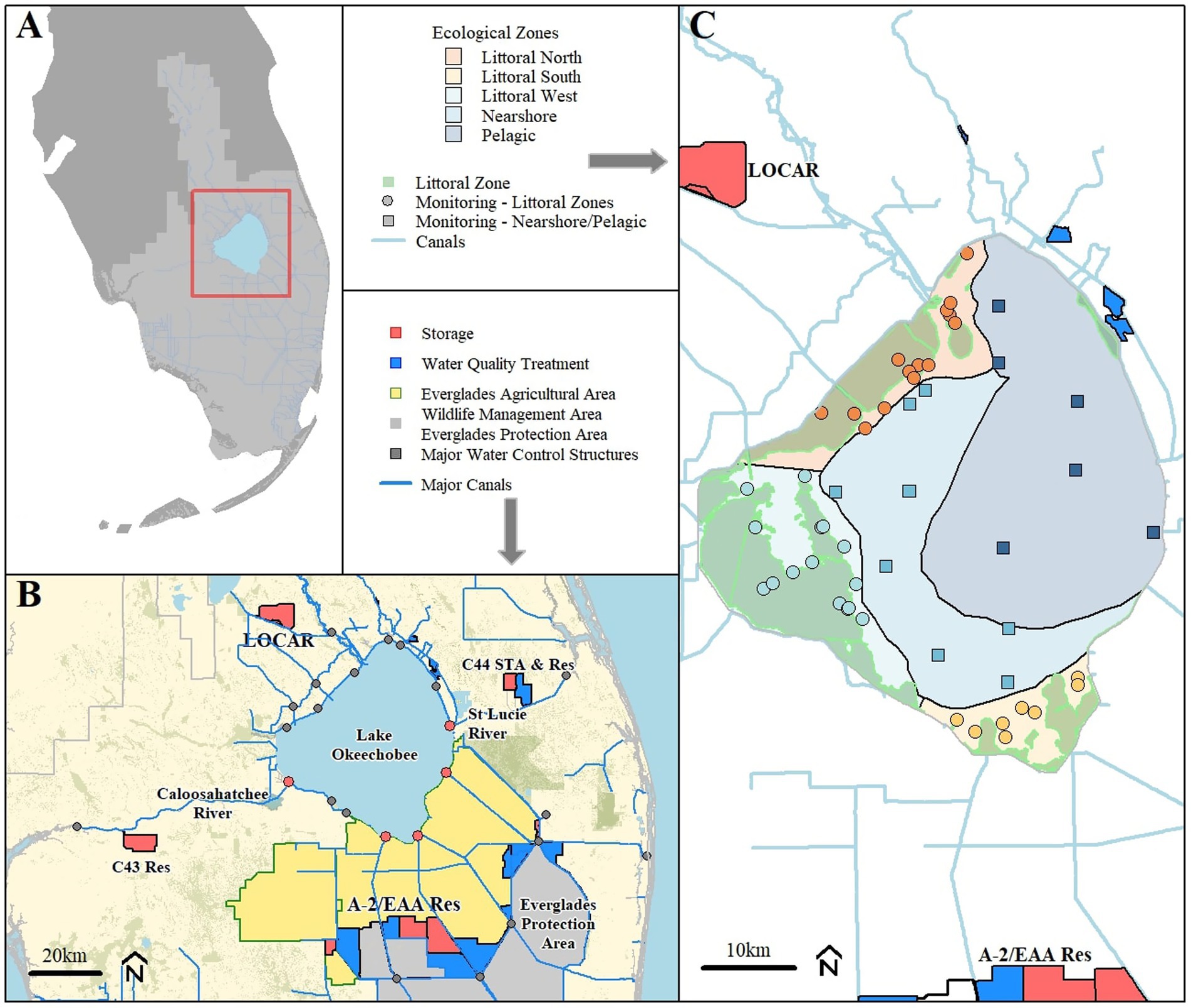
Figure 1. (A) Relative location of Lake Okeechobee within Florida, (B) overview map of important geographic features and restoration projects, and (C) monitoring locations used in this study and delineation of ecological zones, modified from Phlips et al. (1993).

We evaluate the lake as three regions: (1) littoral, (2) nearshore, and (3) limnetic zones. The shallow nearshore and littoral region comprises a third of the total lake surface area and contains a diverse plant community of emergent and submerged aquatic vegetation. The limnetic zone or open water region of the lake makes up the remaining two-thirds of the surface area. This limnetic portion in the central, north, and east has predominately flocculent mud sediments (Fisher et al., 2001; Julian et al., 2023), which are a persistent source of turbidity and nutrients in the lake (Phlips et al., 1993; Harris et al., 2007).

Data sources

Water quality and hydrodynamic data were retrieved from the South Florida Water Management District Online Environmental Database (Table 1) for locations across Lake Okeechobee (Figure 1) between October 1987 and September 2023 (Federal Water Years [WY] 1988 to 2023; Table 1). Nutrient and chlorophyll-a data were collected as surface water grab samples during the period of record. Daily average phycocyanin concentration data were collected from a subset of long-term, near-surface (0.5 m below water surface) monitoring locations (Figure 1) between October 2016 and September 2023. Any data associated with a fatal qualifier indicating a potential data quality problem was removed from the analysis. For data analyses and summary statistics, values reported below the method detection limit (MDL) were assigned a value of one-half the MDL.

Table 1

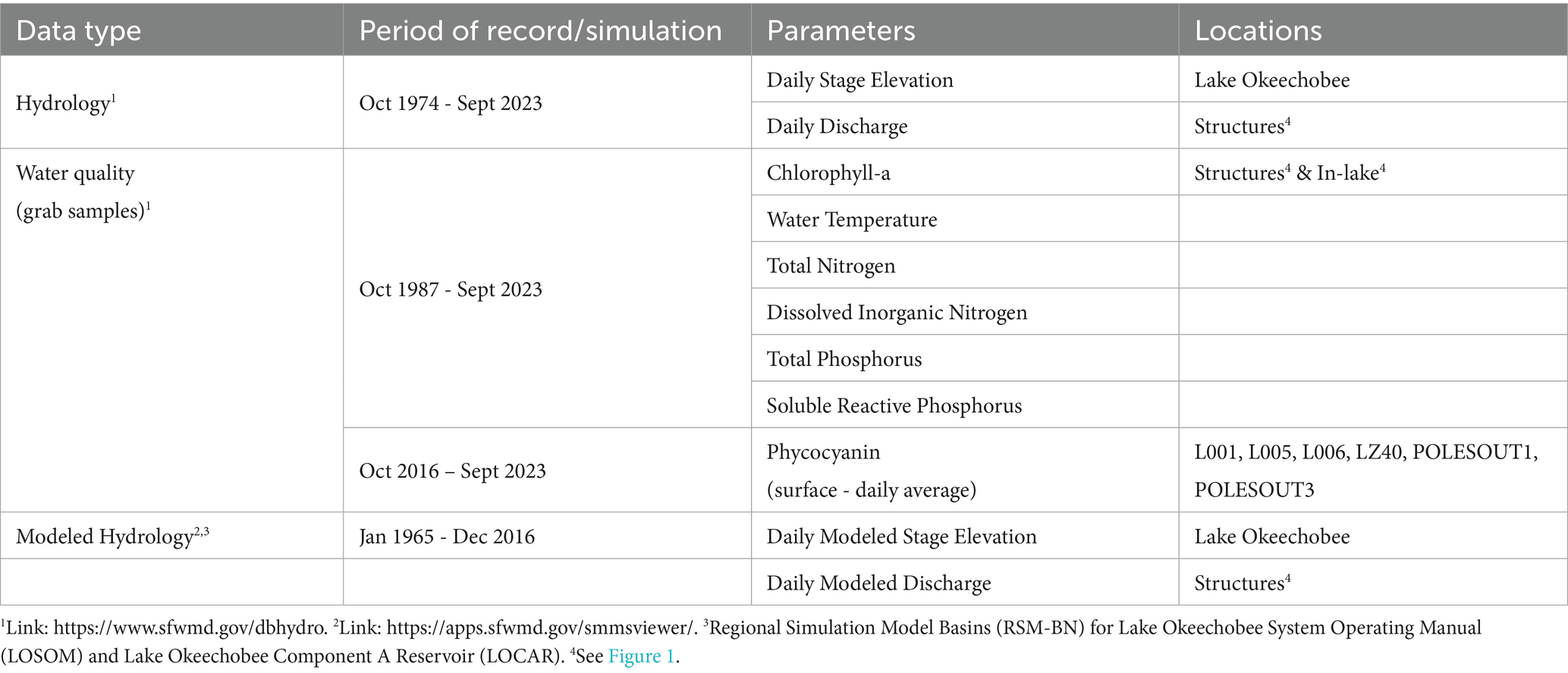
Table 1. Data type, parameters, and sources for data used in this study.

Scenario modeling was conducted using the Regional Simulation Model – Basins (RSM-BN). The RSM-BN model uses past climatology in a link-node framework to simulate hydrologic conditions by using a Hydrologic Simulation Engine (Chin et al., 2005) combined with a Management Simulation Engine (Bras et al., 2019). The RSM-BN model has a 52-year simulation period of record from January 1, 1965 to December 31, 2016. For purposes of restoration planning, the RSM-BN model uses observed variability in climatology across the SFWMD boundary as input to simulate water management changes. Therefore, over the 52-year simulation period, the model includes extreme events such as prolonged drought, hurricanes, tropical storms, and prolonged periods of high and low rainfall. The RSM-BN is a robust simulation tool that has been used in project planning efforts for several projects including the Central Everglades Planning Project, Lake Okeechobee Watershed Restoration Project, Western Everglades Restoration Project, Everglades Restoration Transition Plan, and Combined Operational Plan (South Florida Water Management District, 2020).

This study used the Lake Okeechobee System Operating Manual (LOSOM; US Army Corps of Engineers, 2024a) and the Lake Okeechobee Component a Reservoir (LOCAR; US Army Corps of Engineers, 2024b) RSM-BN based modeling efforts. Both efforts included unique baseline conditions and preferred/selected operational or restoration alternatives. Moreover, project planning and modeling were conducted at different times. In the LOSOM modeling effort, the intention was to evaluate changes in Lake Okeechobee’s regulation schedule, therefore, the no-action 2025 (NA25; equivalent to a future without project baseline) baseline condition assumes the Lake Okeechobee Regulation Schedule of 2008 (LORS08) lake operations. The infrastructure included in the NA25 baseline contained the completion of capital projects and foundational Comprehensive Everglades Restoration Plan (CERP) projects including the rehabilitation of the Herbert Hoover Dike (HHD), operation of the C-44 reservoir (to the east of Lake Okeechobee), and operation of stormwater treatment areas (STAs) downstream of Lake Okeechobee that treat lake water in addition to agricultural runoff. The final alternative was the preferred alternative 2025 (PA25) that represented the completed infrastructure outlined above for the NA25 alternative but also included C-43 reservoir (downstream of the western outlet), and the A-2 stormwater treatment area (downstream of southern outlets) with water management being guided by the new LOSOM regulation schedule (Table 2).

Table 2

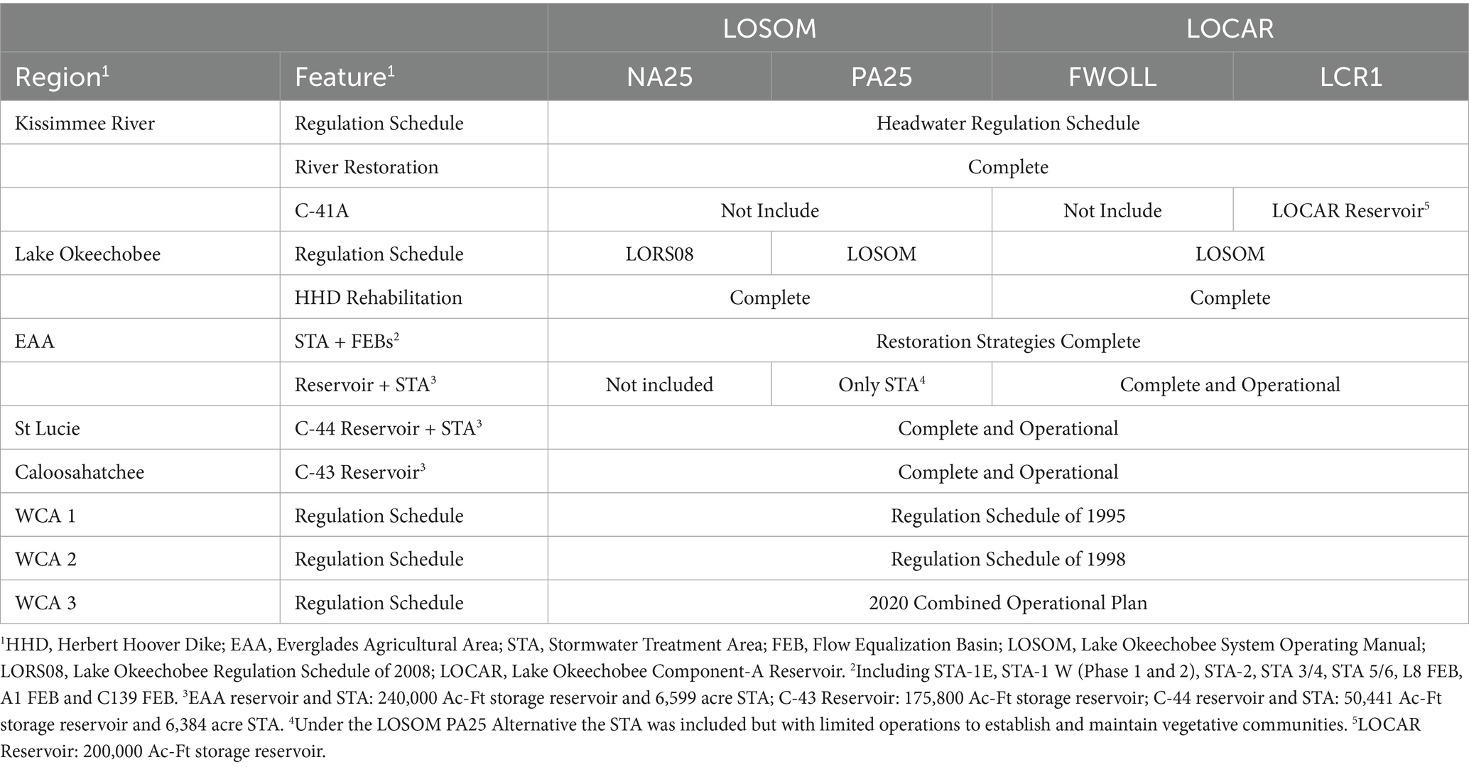
Table 2. Summary of baseline and restoration/operational alternative assumptions for the Lake Okeechobee System Operating Manual (LOSOM) and Lake Okeechobee Component a Reservoir (LOCAR) project.

For the LOCAR modeling effort, the baseline condition (FWOLL) assumes LOSOM water management and regulatory operational guidance for Lake Okeechobee and included the Everglades Agricultural Area (EAA) Reservoir and stormwater treatment area. In the preferred alternative for LOCAR (LCR1), a 200,000 acre-ft storage reservoir located north of Lake Okeechobee was also included. The northern reservoir was modeled to attenuate flows to the lake by capturing wet season flows, and provide supplemental flows during the dry season (USACE, 2024; Figure 1; Table 2).

Generally, LORS08 was a prescriptive operational plan with numerous water level-based management bands that dictated recommended discharge volumes to the major lake outlets. These discharges primarily benefited water supply while providing highly damaging discharges to the Northern Estuaries (Caloosahatchee and St Lucie River estuaries) and starving the Everglades ecosystem to the south (Julian and Reidenbach, 2024). Meanwhile, LOSOM was developed to provide operational flexibility, providing ample water supply benefits while improving salinity regimes for the Northern Estuaries and increasing ecological flows to the southern Everglades (Julian and Welch, 2022; Julian and Reidenbach, 2024).

Data analyses

Ecological zone factor analysis

To assess variations in biogeochemistry and the effect of hydrologic characteristics across the different ecological zones non-metric multidimensional-scaling analysis (NMDS; ‘metaMDS’ function in the vegan R-package; Oksanen and Guillaume, 2018) was used with the Kulczynski dissimilarity index. This approach, rather than other ordination techniques, was selected as this method preserves the rank order of dissimilarities and, therefore, the relationships among zones. The Kulczynski dissimilarity index was used as it is a good index for detecting underlying ecosystem gradients (Faith et al., 1987).

Global and pairwise analysis of similarities (ANOSIM) analyses using the ‘anosim’ (in the vegan R-package) and ‘anosim.pw’ (see supplemental) functions was conducted to test statistically whether there were significant differences between ecological zones. Variables included in these analyses were spatially averaged by ecological zone annual (WY) geometric mean concentrations of TP, TN, SRP, DIN, chlorophyll-a, surface water temperature, annual average stage elevation, storage volume, water residence time (WRT), total inflow discharge volume, TP load and TN Load, and total in-lake TP and TN load by zone.

Annual inflow nutrient loads were estimated by interpolating nutrient concentrations daily from grab samples collected at each respective water control structure during days of observed discharge. Daily interpolated nutrient concentrations were multiplied by daily flow and summed for each WY. Annual total in-lake nutrient loads were estimated for each monitoring location by determining a site-specific water depth based on lake stage and lake bottom (from lake bathymetry) for each sample. Water depth was multiplied by nutrient concentration and annual average computed to produce an annual average areal load.

The annual average load was then spatially averaged across the ecological zone and multiplied by ecological zone area. The annual average storage volume was estimated from the stage-area-volume curve, which was estimated from spatial bathymetric data combined with daily stage data and average over the water year. Annual average water residence time was calculated by dividing the annual average storage volume by the total annual outflow volume.

Pigment trend analyses

To evaluate seasonal trends and spatial variability of chlorophyll-a and phycocyanin pigment concentrations across Lake Okeechobee, spatiotemporal generalized additive models (GAM; mcgv R-package; Wood, 2017) were fit for chlorophyll-a and phycocyanin, separately using the ‘bam’ function. Due to significant differences in how Lake Okeechobee was managed between regulation schedules (Tarabih and Arias, 2021; Julian and Welch, 2022; Julian et al., 2024), this evaluation of chlorophyll-a will focus on the 2008 to 2023 period of record. The model was constructed consistent with Equation 1 for chlorophyll-a and Equation 2 for phycocyanin. Differences in model variables, smoothing functions, and interaction effects were necessary due to differences in the frequency of data collection, spatial coverage, and time-series duration. The chlorophyll-a model was fit using the Gaussian log-linked distribution. Meanwhile, the phycocyanin model was fit using the Tweedie distribution. Model fit distributions were selected based on data distribution, model residual distributions, and overall model fit.

$\begin{array}{l}E\left(\mathit{Chl}{a}_t\right)=\alpha +s\left(\mathit{\text{stage}}\right)+s\left(\mathit{\text{decMonth}}\right)+s\left(\mathit{CY}\right)\\ +s(\mathit{\text{Long}},\mathit{Lat})+\mathit{ti}(\mathit{CY},\mathit{\text{decMonth}})\\ +\mathit{ti}(\mathit{\text{Long}},\mathit{Lat},\mathit{\text{decMonth}})+\mathit{ti}(\mathit{\text{Long}},\mathit{Lat},\mathit{CY})\end{array}\text{ (1)}$

$\begin{array}{l}E\left({\mathit{\text{Phyco}}}_t\right)=\alpha +s\left(\mathit{\text{stage}}\right)+s\left(\mathit{\text{decYr}}\right)+s\left(\mathit{DOY}\right)\\ +s(\mathit{\text{Long}},\mathit{Lat})+\mathit{ti}(\mathit{\text{Long}},\mathit{Lat},\mathit{\text{decYr}})\end{array}\text{ (2)}$

Degrees of smoothing (knots = k) were initially used to minimize the generalized cross-validation score, followed by post hoc adjustments of ‘k’ for individual terms using the function ‘gam.check’. The first derivative of the fitted trend was evaluated using finite differences (gratia R-package; Simpson, 2021). Periods of significant change were identified when the confidence interval of the first derivative for the fitted stage, year and decimal month spline for the chlorophyll-a model and stage, day-of-year and decimal year spline for the phycocyanin model spline did not include zero, consistent with Simpson (2018).

Algal bloom risk tool

To develop a simple predictive framework to evaluate changes in chlorophyll-a concentrations and algal bloom risk across Lake Okeechobee a series of models were developed to support restoration planning efforts consistent with Walker (2020). The models include summer (May–August) mean chlorophyll-a concentration, and bloom frequency as defined by exceeding chlorophyll-a concentrations of 20 μg L⁻¹ (f_Chla20) and 40 μg L⁻¹ (f_Chla40). Data between October 1999 and September 2023 were used to fit the concentration and bloom frequency models with years of major hurricanes excluded (WYs 2000, 2004, 2006, 2017, and 2022).

Bloom condition thresholds were based on Lake Numeric Nutrient Criteria (i.e., 20 μg L⁻¹ for high color and alkalinity lakes) (Florida Administrative Code, 2016a, 2016b) and prior Lake Okeechobee algal studies (i.e., 40 μg L⁻¹) (Havens, 1994; Walker and Havens, 1995; Havens and Walker, 2002). Seasonal annual mean chlorophyll-a and exceedance frequencies (f_Chla20 and f_Chla40) were estimated for each location across the lake followed by a spatial aggregation by ecological zones (Figure 1) adapted from Phlips et al. (1993). These spatial aggregations reflect a combination of unique characteristics such as sediment types, vegetative communities, and average depth.

Ecological zone annual summer mean chlorophyll-a concentrations and exceedance frequencies (f_Chla20 and f_Chla40) were fit to summer mean lake stage elevation constrained to a minimum value of 3.5 meters National Geodetic Vertical Datum 1929 (NGVD29; 11.5 feet) using a mixed effect model framework with the ‘gam’ function of the ‘mgcv’ R-package, incorporating random effects smooths. The models were specified with constrained stage as the fixed effect and ecological zone as a random effect to account for random slope and intercepts. The chlorophyll-a concentration mixed effect model was fit using the Tweedie distribution and the exceedance frequency models were fit using the binomial logit linked distribution. Since no unified method to estimate conditional (entire model) and marginal (fixed effects only) goodness of fits (i.e., R²) are available for mixed effect models using the ‘mgcv’ package, a fixed effect only and entire model were fit separately to approximate conditional and marginal deviance explained. All models were validated using a k-fold procedure with a total of 5-folds, resulting in an approximately 20% testing and training split. Validation performance indicators used to evaluate the models include average mean absolute error (MAE), root mean square error (RMSE), and mean bias error (MBE). For completeness metric equations, hypothetical ranges and ideal values/goals are included in Supplementary Table S1.

The stage constraint was applied to daily summer stage elevations due to the low frequency of data below 3.5 m (2 out of 17 years used in the analysis) and the variability of chlorophyll-a concentrations across regions (Walker, 2020). This variability could be related to the difficulties in obtaining representative samples in shallow water depths and the spatial heterogeneity of water quality conditions under low-stage conditions.

Biogeochemical algal model

A second modeling approach was considered to evaluate summer average chlorophyll-a concentrations across the different ecological zones to assess the relative change in conditions across model alternatives. This modeling approach considered hydrodynamic and biogeochemical characteristics informed by the results of the NMDS evaluation and prior lake modeling studies (Olson and Jones, 2022; Hanson et al., 2023). Using the same period as identified above for the stage-based mixed models (October 1999 – September 2024 with hurricane years excluded). Summer average chlorophyll-a concentration data were fitted. The variables considered include summer mean TP, DIN concentrations, water residence time (WRT), depth (z), inflow discharge volume (Q_in), and ecological zone (Equation 3) in a hierarchical GAM (HGAM) framework (Pedersen et al., 2019) with parametric, smoothing (s), and tensor interaction (ti) terms. Due to the dependency of TP and DIN concentrations in the summer average chlorophyll model (Equation 3), two additional models were also fit to predict summer average TP and DIN concentrations (Equations 4, 5, respectively) using hydrodynamic predictor variables (lake volume [V], and outflow discharge volume [Q_out]) across ecological zones. Given the distribution of the data, chlorophyll and TP models were fitted using the Tweedie distribution with a log link while the Gamma distribution with a log link was applied to the DIN model. Models were tested using observed data between October 1976 and September 1999 with hurricane years excluded. Models were tested using several goodness of fit metrics including R² between the observed vs. predicted during the testing period Kling Gupta model efficiency (KGE; Supplementary Table S1; Gupta et al., 2009), and absolute model fit metric used above (i.e., MAE, RMSE, and MBE). Finally, models were validated using the leave-one-out cross-validation (LOOCV) procedure and assessed using MAE, RMSE and MBE as validation performance indicators.

$\begin{array}{l}E\left(\mathit{Chl}{a}_{\mathit{sum}}\right)=\alpha +\mathit{WRT}+\mathit{TP}+\mathit{DIN}+\mathit{ti}(\mathit{TP},\mathit{DIN},\mathit{\text{EcoZone}})\\ +s\left(z\right)+s\left(Q_{\mathit{\text{in}}}\right)+s\left(\mathit{\text{Ecozone}}\right)\end{array}\text{ (3)}$

$\begin{array}{ll}E\left(T{P}_{\mathit{sum}}\right)=\alpha +s(V,\mathit{\text{EcoZone}})+s\left(Q_{\mathit{\text{out}}}\right)+s\left(\mathit{\text{Ecozone}}\right)& (4)\end{array}$

$\begin{array}{ll}E\left(\mathit{DI}{N}_{\mathit{sum}}\right)=\alpha +Q_{\mathit{\text{out}}}+V+s(\mathit{WRT},\mathit{\text{EcoZone}})+s\left(\mathit{\text{Ecozone}}\right)& (5)\end{array}$

Application of algal risk models

Modeled stage elevation values for the entire period of simulation and summer only for all unique combinations of modeled scenarios were evaluated using the two-sample Anderson-Darling test (Anderson and Darling, 1952; Pettitt, 1976) using the ‘ad.test’ function in the ‘kSamples’ R-Package (Scholz and Zhu, 2023). To evaluate if simulated stage elevations were significantly different between alternatives considered in this study, a total of six unique comparisons were made (Supplementary Table S2). Other distribution comparison statistics such as the Kolmogorov Smirnov test (‘ks.test’) can become too sensitive in large sample sizes (high type II error) when computing test statistics and associated probabilities due to the high sample size of daily simulated stage values; therefore, the Anderson-Darling test was considered.

Using annual summer average stage elevations for each alternative, chlorophyll-a concentration, f_Chla20, and f_Chla40 were predicted for the entire period of simulation. For alternative comparison purposes, the average percent difference of chlorophyll-a concentration, f_Chla20, and f_Chla40 was calculated for each ecological zone between project alternatives to evaluate the integrated effect of changes in water management and the addition of storage capacity within the system. To avoid pseudo replication of estimated values, predicted chlorophyll-a concentration, f20_Chla, and f40_Chla from fixed effects were compared between alternatives using Pairwise Wilcoxon Rank Sum Test (‘pairwise.wilcox.test’ in the base R-package) with p-values being adjusted using the Holm-Bonferroni method. The fixed effects model, often called the “mean model” or “within estimator,” refers to the variation between groups. Therefore, in the case of this study, it better represents a comparison between model alternatives. Like the stage-based model, the Lake Okeechobee hydrodynamic and biogeochemical chlorophyll hierarchal additive zonal model (Equations 3–5; LOK HABAM) compared the average percent difference of predicted chlorophyll-a concentrations for each ecological zone between restoration and operations scenarios.

Due to the nature of GAMs, sharing a simple equation for future use in other code/object-oriented programs or spreadsheet-based platforms is not feasible, a shiny application (and source code) has been developed to extend the functionality of the models presented here. The stage-based mixed models and LOK HABAM predictive functionality is provided as an interactive application¹ where model alternatives presented in this study or future alternatives can be evaluated. The source code for this shiny application is available in a public repository.²

All statistical operations were performed with R © (Ver 4.1.0, R Foundation for Statistical Computing, Vienna Austria). Unless otherwise stated, all statistical operations were performed using the base R library. The critical level of significance was set at α = 0.05.

Results

Ecological zone factor analysis

Results from the NMDS demonstrated a clear separation of ecological regions for in-lake characteristics, in-lake load estimates, stage and lake inputs (inflow discharge volume and nutrient loading; Figure 2) with a stress value of 0.14 for the first two dimensions with a relatively high non-metric and linear fit R² values of 0.98 and 0.91, respectively (Supplementary Figure S1). Inflow discharge was linked to inflow TP and TN loads, while stage, volume, WRT, TN, temperature, and chlorophyll-a were also interrelated. Meanwhile, TP, SRP, and DIN concentrations were generally associated. Ecological regions were stretched across the first NMDS axis with the littoral zones clustering and pelagic and nearshore zones forming separate, distinct groups (Figure 2). This observed grouping of ecological zones was confirmed by ANOSIM, showing a significant global difference between groups and significant pairwise differences between pelagic/nearshore and littoral zones, while littoral zones were not significantly different from one another (Table 3).

Figure 2

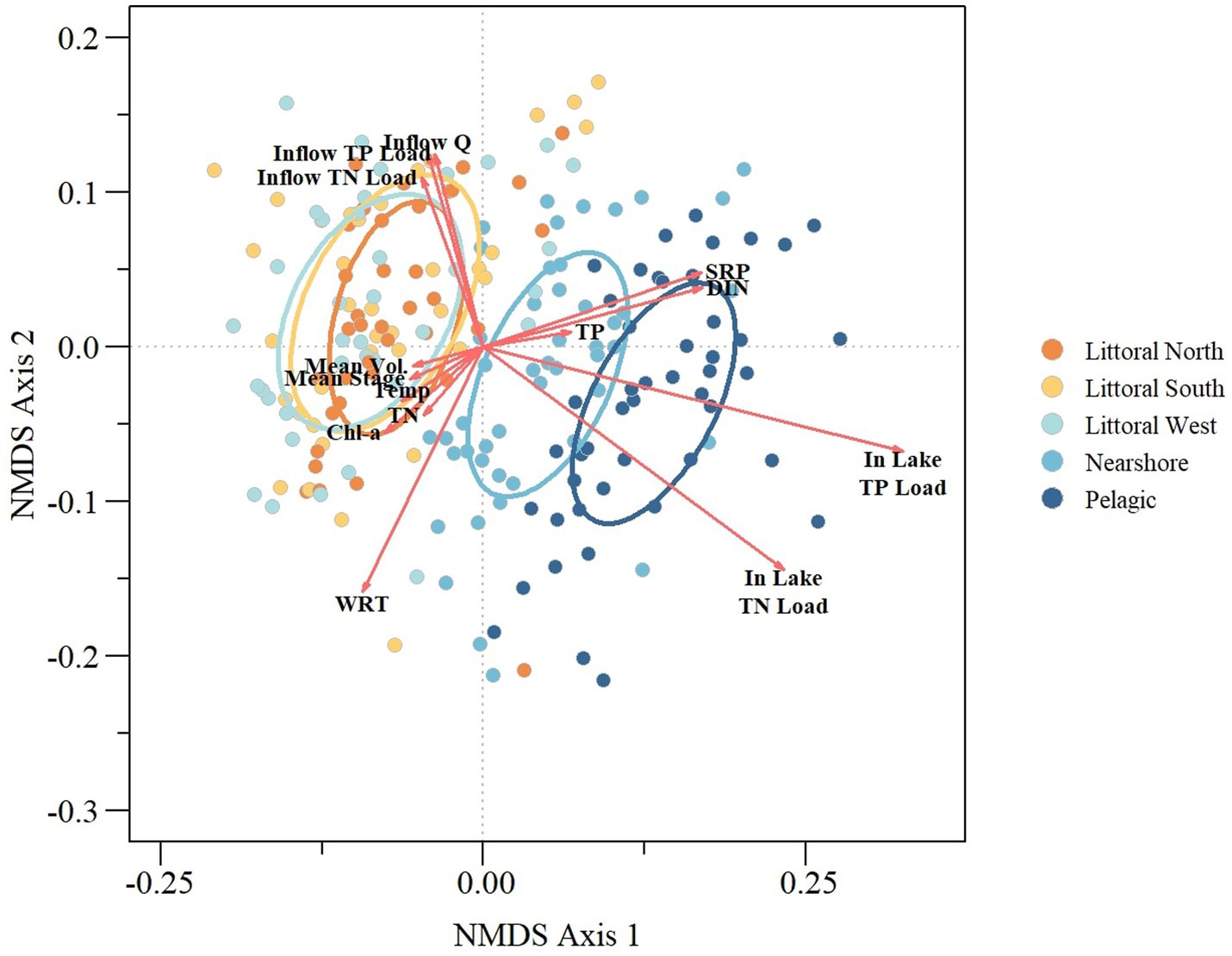
Figure 2. Nonmetric dimensional scaling (NMDS) biplot of in-lake and lake input parameters relative to lake ecological regions. Ordination ellipses are based on 95% confidence limit of the NMDS sites score.

Table 3

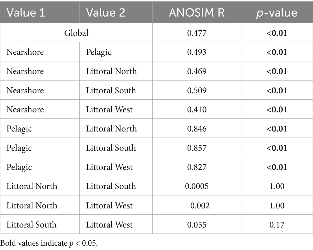
Table 3. Analysis of similarities results including global (overall) and pairwise comparisons between ecological zones in Lake Okeechobee.

Pigment trend models

Chlorophyll-a concentrations varied across space, time, and stage (Figures 3A–D) with the GAM explaining 75% of the deviance (relative to a null model) and an R² of 0.69 (Table 4). The spatial effect of the model (Figure 3D) varied across the lake with the largest spatial effect located in a region of the southwestern edge of the lake while the lowest spatial effect was adjacent to the southern part of the pelagic zone (Figures 1, 3D). Temporally, within year (i.e., monthly) effects were greatest in the summer months peaking around July with significant increases being detected between April and June and significant decreases between October and later November (Figure 3B). Between-year effects (Figure 3C) varied with some notable fluctuations after major hurricanes and other climatic events. For example, the annual effect significantly declined after 2008 following a tropical storm that relieved regional drought conditions, but increased, while not significant following 2017 (year of Hurricane Irma). The effect of stage elevation varied across the observed range of stage conditions during the 2008 to 2023 POR, with a significant increase between 3.57 and 3.96 m NGVD29 and a significant decrease between 4.91 and 5.15 m NGVD29 (Figure 3A).

Figure 3

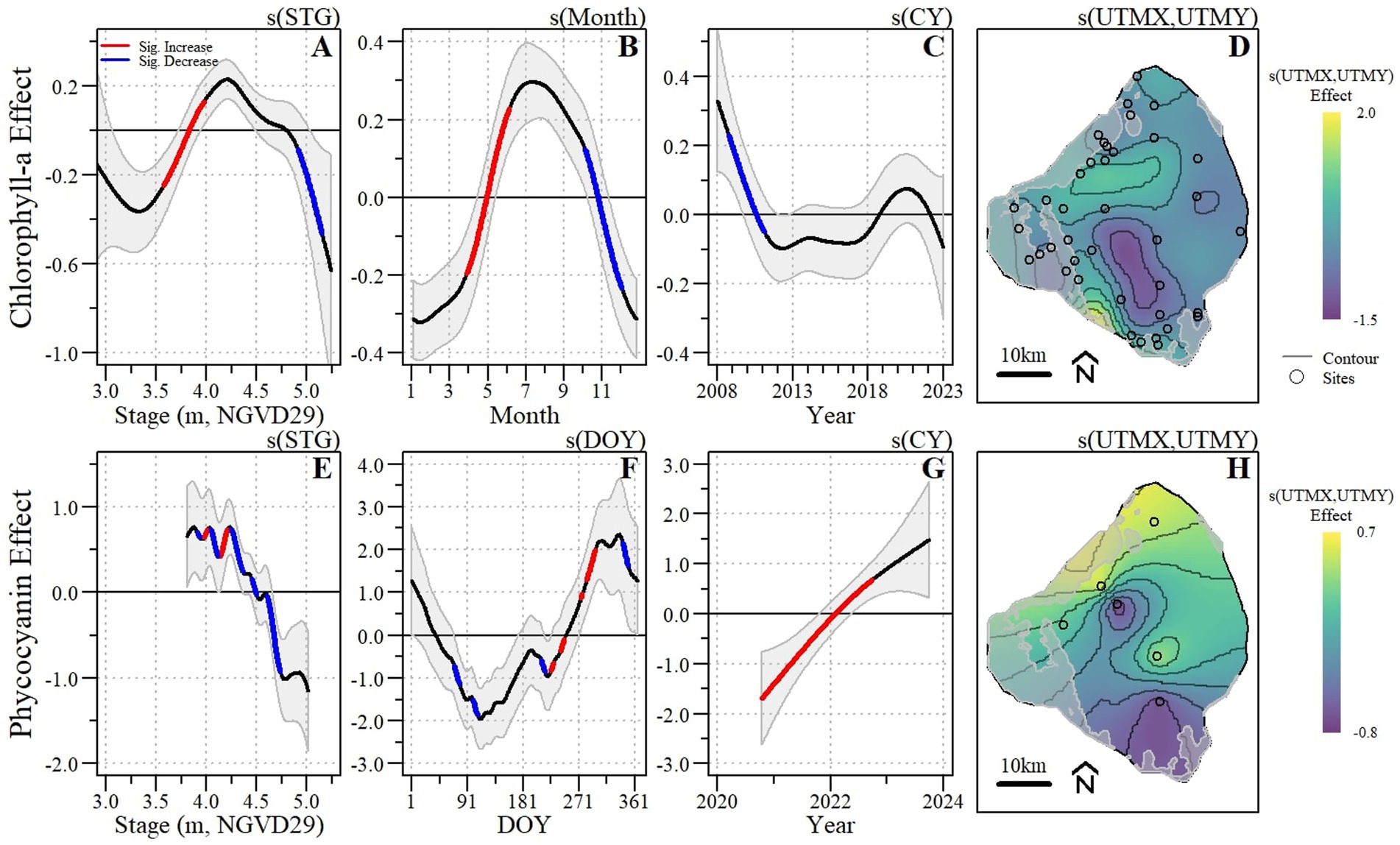
Figure 3. Chlorophyll-a (A–D) and phycocyanin (E–H) spatio-temporal generalized additive model effect plots for stage (A,E), short-term/within-year (B,F), long-term/annual (C,G) and spatial (D,H) effects with significant changes identified. For each respective effect, splines with significantly increasing and decreasing segments are indicated by red and blue line segments, respectively. Each spline represents the smoothed parameter, along with its 95% confidence interval.

Table 4

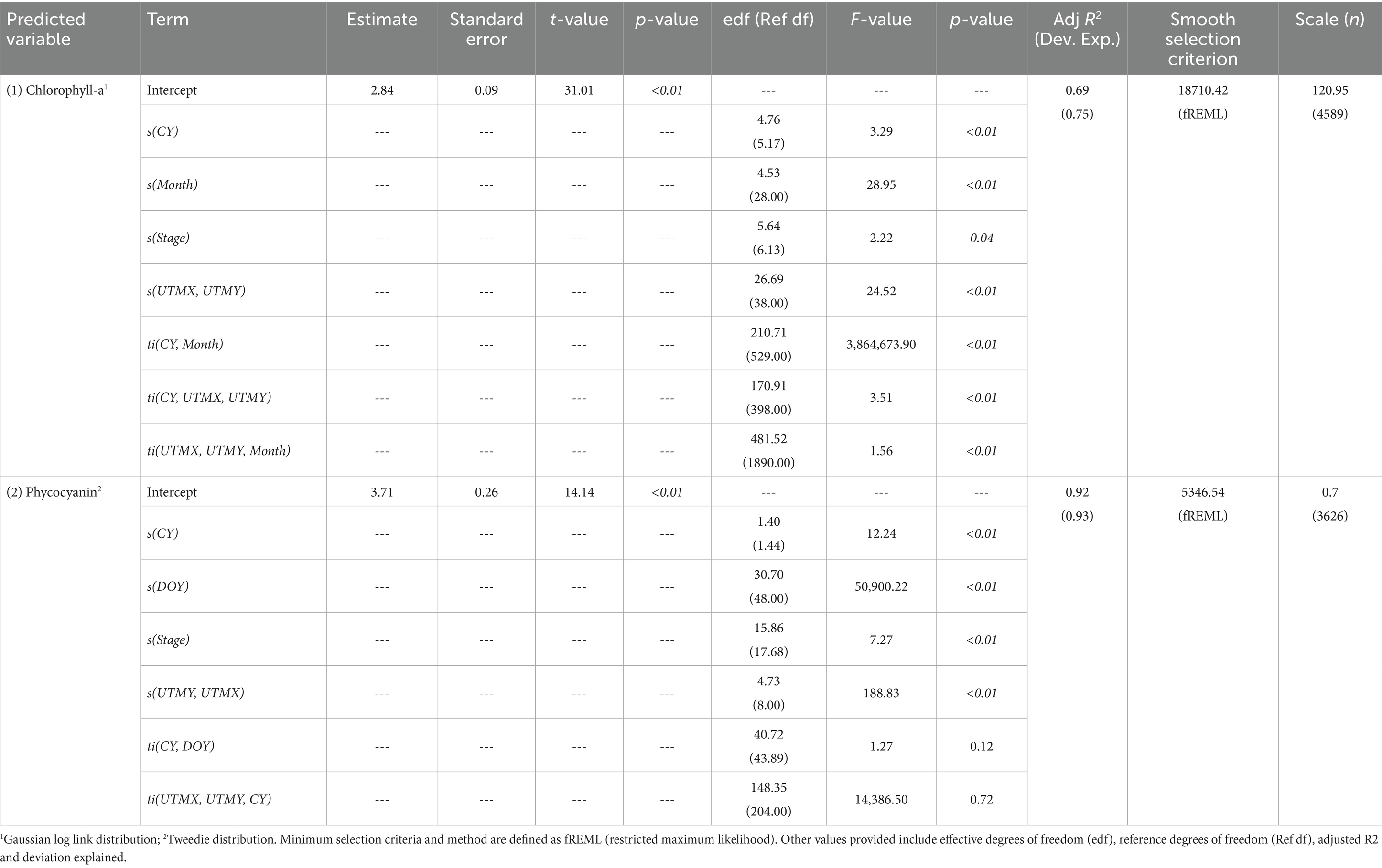
Table 4. Spatio-temporal generalized additive model results for chlorophyll-a (1) and phycocyanin (2) pigment concentration within Lake Okeechobee.

Despite the much shorter period of record and spatial coverage, variation in phycocyanin concentrations across space, time, and stage were also detected (Figures 3E–H) with the model explaining 93% of the deviance and an R² of 0.92 (Table 4). The spatial effect of the model (Figure 3H) varied across the lake with the greatest spatial effect along the northern littoral zone and at the center of the lake and the lowest adjacent to the northern and southern littoral zone edge (nearshore zone). Temporally, within-year (i.e., DOY) effects were greatest at the start and end of the year with a double peak in within-year effect with the first smaller peak occurring near the end of July/beginning of August followed by a significant increase and the second peak near the beginning of December. A significant increase in annual effect was detected between late 2020 and late 2022 (Figure 3G). Despite the relatively short time series, significant changes in model effect were also detected relative to stage elevation with a consistent relative decline starting after 4.25 m NGVD29 (Figure 3E). However, due to the short time-series, the stage effect curve was truncated relative to the longer POR for the chlorophyll model therefore the relationship between phycocyanin concentrations and stage is uncertain when stages are less than 3.81 m NGVD29.

Algal risk tool

Due to the limited temporal and spatial coverage of phycocyanin concentrations and the truncated stage conditions, a predictive equation was not developed. The effect of lake stage (constrained to 3.5 m) on summer mean chlorophyll-a concentrations was significant, with a coefficient of 0.178 (SE = 0.089; t-value = 2.0; p-value<0.01; Table 5; Figure 4). The random effect of the ecological zone was significant with respect to random effect on chlorophyll-a concentrations (F = 519.1; p-value <0.01) and chlorophyll-a and stage (F = 332.9; p-value <0.01) with a variance of 0.279 and 0.035, respectively. The deviance explained by the entire model (i.e., conditional deviance explained) was 0.47 (Table 5) meanwhile the deviance explained by just the fixed effects (i.e., marginal) was 0.12. The average MAE, RMSE, and MBE of the five-fold validation were 7.24, 9.24, and 0.27, respectively.

Table 5

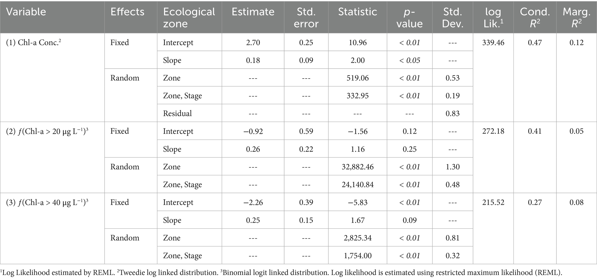
Table 5. Mixed effect model summary for chlorophyll-a concentration (1), frequency of exceeding 20 μg L^–1 (2), and frequency of exceeding 40 μg L^–1 (3) within Lake Okeechobee across ecological zones.

Figure 4

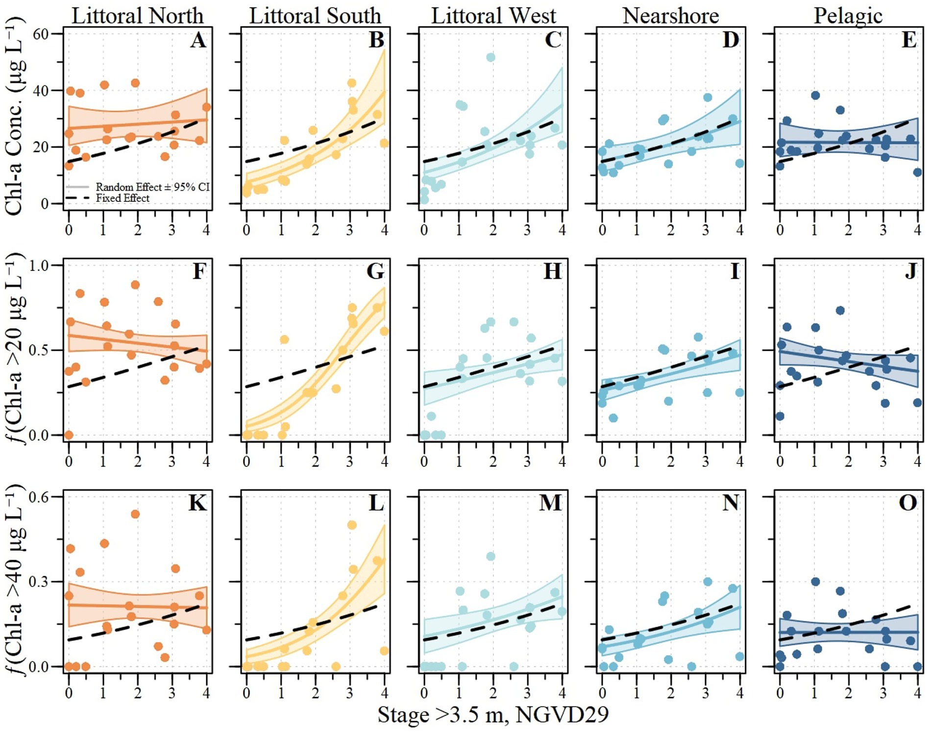
Figure 4. Summer mean Chlorophyll-a concentration (A–E), frequency of exceeding 20 μg L⁻¹ (f_Chla20; F–J), and frequency of exceeding 40 μg L⁻¹ (f_Chla40; K–O) for the five ecological zones across Lake Okeechobee. Random effect (i.e., ecological specific models; line with shading) and fixed effect (black dashed line) relative to observed values between water years 2000 and 2023 with hurricane years excluded (water years: 2000, 2004,2006,2017, and 2022).

The effect of lake stage (constrained to 3.5 m) on summer f_Chla20 was not significant, with a coefficient of 0.263 (SE = 0.1973; z-value = 1.33; p-value = 0.18; Table 5; Figure 4). However, the ecological zone had a significant random effect on f_Chla20 (χ² = 14,542,575; p-value <0.01) and f_Chla20 and stage (χ² = 13,042,007; p-value <0.01) with a variance of 1.68 and 0.235, respectively. The deviance explained by the entire model (i.e., conditional deviance explained) was 0.42 (Table 5) meanwhile the deviance explained by just the fixed effects (i.e., marginal) was 0.05. The average MAE, RMSE, and MBE of the five-fold validation were 0.14, 1.81, and 0.02, respectively.

The effect of lake stage (constrained to 3.5 m) on summer f_Chla40 was not significant, with a coefficient of 0.25 (SE = 0.15; z-value = 1.68; p-value = 0.09; Table 5; Figure 4). The ecological zone had a significant random effect on f_Chla40 (χ² = 2,825; p-value <0.01) and f_Chla40 and stage (χ² = 1754; p-value <0.01) with a variance of 0.660 and 0.100, respectively. The deviance explained by the entire model (i.e., conditional deviance explained) was 0.27 (Table 5) meanwhile the deviance explained by just the fixed effects (i.e., marginal) was 0.08. The average MAE, RMSE, and MBE of the five-fold validation were 0.10, 0.13, and 0.02, respectively.

Biogeochemical algal model

Summer average chlorophyll-a varied significantly between ecological regions, with water depth being a significant effect for nearshore and littoral west ecological zones (Supplementary Table S4). Additionally, TP and DIN parametric terms were significantly different from zero (Supplementary Table S4), while the interaction of TP and DIN did not significantly vary between ecological regions, including it in the model did improve the predictive capabilities of the model. However, TP and DIN interaction and mean depth by ecological zone resulted in a non-linear relationship for most ecological regions (based on effective degrees of freedom (edf) values; Supplementary Table S4). For the testing dataset, the chlorophyll-a model resulted in an R² of 0.51 (observed vs. predicted during the training period), KGE of 0.59, MAE of 5.61 μg L⁻¹, RMSE of 7.45 μg L⁻¹_, and MBE of −2.83 μg L⁻¹. For validation, the MAE, RMSE, and MBE were 8.75, 11.29, and −0.47 μg L⁻¹, respectively as estimated by the LOOCV procedure. The resulting model produced a model fit (R²_adj) of 0.70 and a deviance explained of 83.5% (Supplementary Table S4).

Summer average TP concentration varied between ecological zones, outflow discharge volume, and lake volume for most ecological zones (littoral south, littoral west, and nearshore; Supplementary Table S4). Based on the edf values of the lake volume by ecological zone smoothing terms, summer TP was linear and not significantly different from zero for littoral north and pelagic zones, the nearshore zone was linear but significantly different from zero (with a slight positive slope based on first derivative values) and the littoral south and littoral west were non-linear. For the testing dataset, the TP model resulted in an R² of 0.45, KGE of 0.49, MAE of 0.040 mg L⁻¹, RMSE of 0.044 mg L⁻¹_, and MBE of 0.038 mg L⁻¹. For validation, the MAE, RMSE, and MBE were 0.042, 0.052, and −0.0002 mg L⁻¹, respectively as estimated by the LOOCV procedure. The resulting model produced a model fit (R²_adj) of 0.64 and a deviance explained of 70.8% (Supplementary Table S4).

Summer average DIN concentrations varied between ecological zones, outflow discharge volume, and WRT, specifically within the littoral north zone. For the testing dataset, the DIN model resulted in an R² of 0.32, KGE of 0.22, MAE of 0.039 mg L⁻¹, RMSE of 0.048 mg L⁻¹_, and MBE of 0.025 mg L⁻¹. For validation, the MAE, RMSE, and MBE were 0.078, 0.100, and −0.009 mg L⁻¹, respectively as estimated by the LOOCV procedure. The resulting model produced a model fit (R²_adj) of 0.58 and a deviance explained of 61.2% (Supplementary Table S4).

Application of algal risk models

Over the simulation periods, among the four alternatives, daily stage elevation ranged from 2.5 to 5.4 m (NGVD29; Supplementary Table S5). Daily stage distributions among alternatives were significantly different (Table 6; Figure 5). Generally, NA25 has the lowest stage elevations while PA25 is the highest with the greatest difference in the two stage duration curves (or cumulative distribution curves) occurring at 4.75 m NVGD29 (Figures 5A,C,D). Meanwhile, the FWOLL and LCR1 stage duration curves fell between those of NA25 and PA25, with the latter two being closer together but showing a notable shift in stage timing (Figures 5B,E,F). LCR1 further reduced high stages and decreased the occurrence of relatively low stage conditions (<4.0 m NGVD29). The greatest difference between FWOLL and LCR1 occurred at 3.65 m NGVD29 (Figure 5B).

Table 6

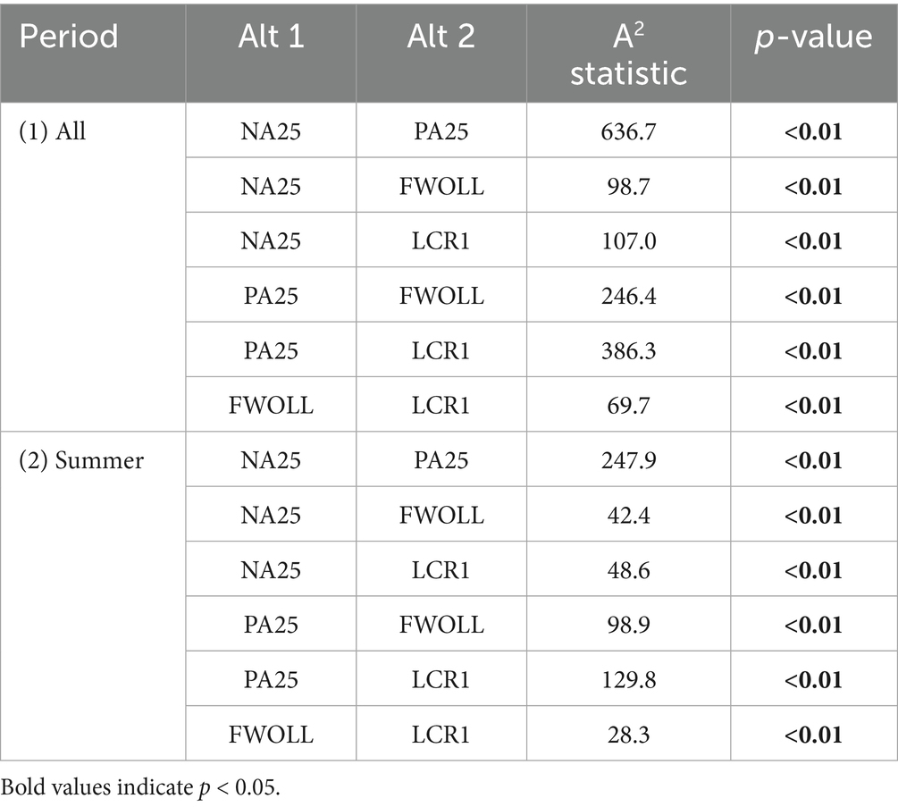
Table 6. Comparison of daily stage elevations over the entire period of simulation (1) and summer only (2) between all unique combinations of alternatives using the two-sample Anderson-Darling test.

Figure 5

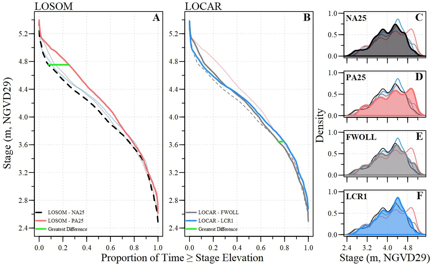
Figure 5. Stage duration curves for (A) the Lake Okeechobee System Operating Manual evaluation between the baseline (NA25) and preferred alternative (PA25) and (B) the Lake Okeechobee Component a Reservoir evaluation between baseline (FWOLL) and preferred alternative (LCR1) with the greatest difference in duration curves identified. For comparison, each plot has all alternatives presented but de-emphasized depending on the focus (i.e., LOSOM (A) presents both LOSOM and LOCAR with LOCAR alternatives in a light shade of color). Density plots of daily stage elevation during the period of simulation for (C) NA25, (D) PA25, (E) FWOLL, and (F) LCR1.

Mean predicted chlorophyll-a concentrations ranged from 7.6 to 55.6 μg L⁻¹ for random effects (ecological zones) and 14.9 to 35.1 μg L⁻¹ for fixed effects (Supplementary Table S6). Predicted f_Chla20 values ranged from 0.05 to 0.89 (proportion) for random effects and 0.29 to 0.58 for fixed effects (Supplementary Table S6). Finally, predicted f_Chla40 values ranged from 0.03 to 0.52 for random effects and 0.09 to 0.26 for fixed effects (Supplementary Table S6). In most cases, chlorophyll-a concentration, f_Chla20, and f_Chla40 increased between NA25 and PA25, with the greatest difference in all variables observed in the Littoral South ecological region (Figure 6; Table 7). For most ecological regions, chlorophyll variables showed a relative decrease or remained unchanged (±5%) between PA25 and FWOLL, as well as between FWOLL and LCR1 alternatives (Figure 6; Table 7). Finally, the comparison between PA25 and LCR1 indicated a decrease or relatively no change in bloom conditions across ecological zones (Figure 6, Table 7).

Figure 6

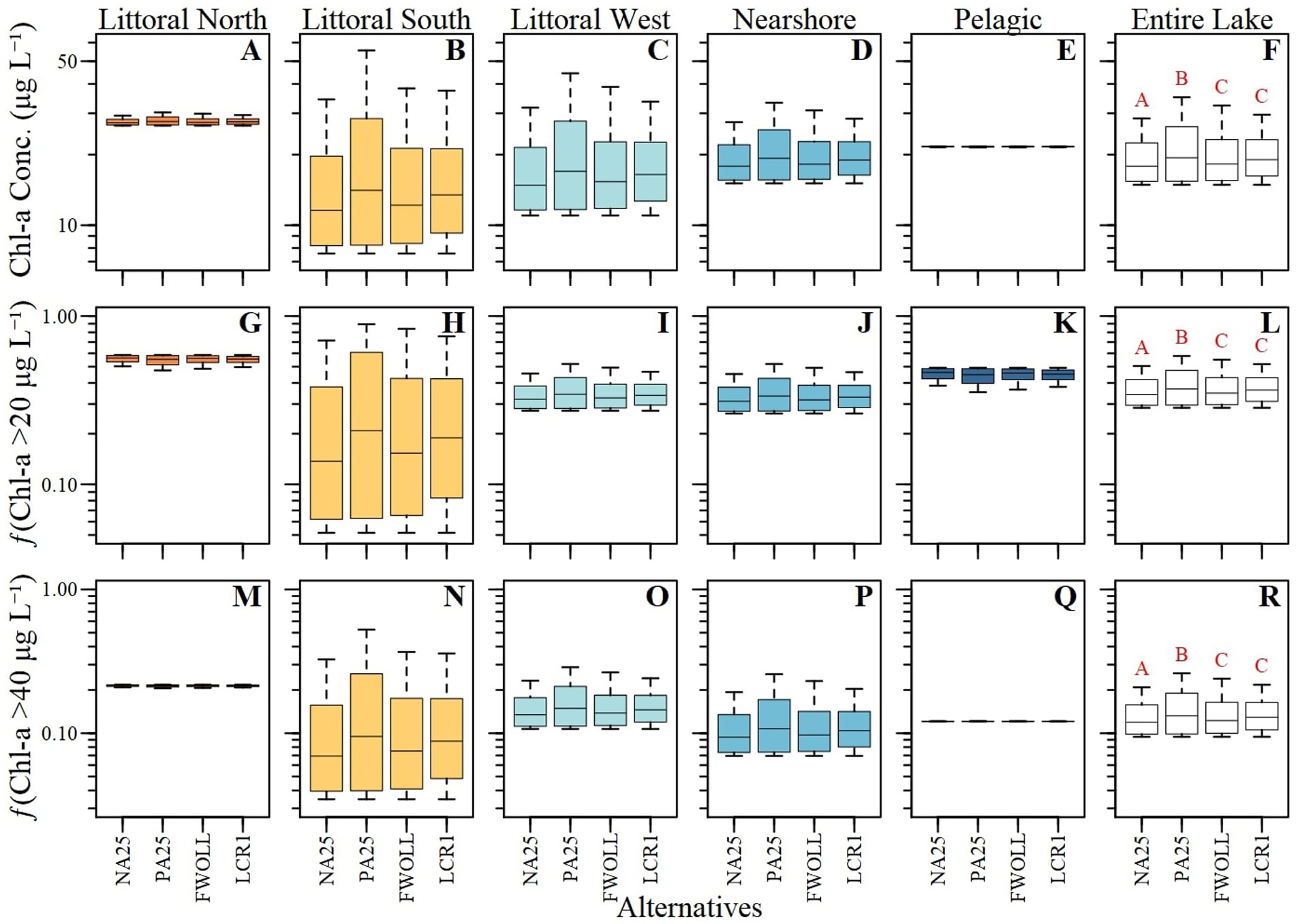
Figure 6. Boxplot of the 52-year period of simulation for each ecological zone (A–E, G–K and M–Q; i.e. random effects) and lake-wide (F,L and R; fixed effect) predictions of chlorophyll-a concentration (A–F), frequency of exceeding 20 μg L⁻¹ (G–L) and frequency of exceeding 40 μg L⁻¹ (M–R) across Lake Okeechobee and alternatives.

Table 7

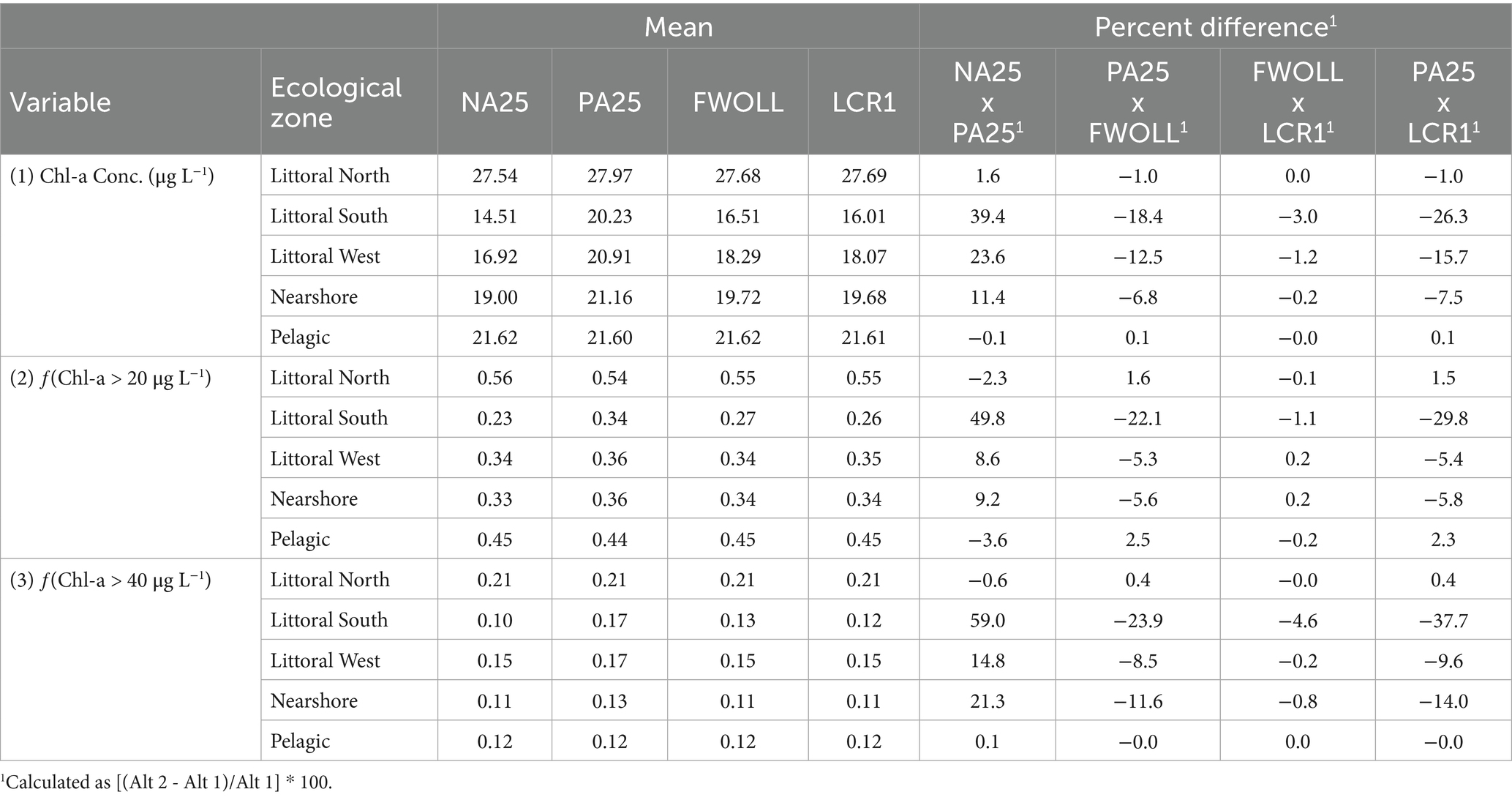
Table 7. Period of simulation mean and mean percent difference of predicted chlorophyll-a concentration (1), frequency of exceeding 20 μg L^–1 (2), and frequency of exceeding 40 μg L^–1 (3) across ecological zones and alternatives.

All chlorophyll parameters (i.e., concentration, f_Chla20, and f_Chla40) varied among alternatives (Supplementary Table S7) and across ecological zones (Supplementary Table S7; Figure 6). Since the models were developed using the annual summer average stages, each variable exhibited similar responses specific to the parameter of interest. Generally, the littoral north and pelagic zones exhibited the least variability in predicted chlorophyll concentrations and bloom categories (Figures 6A,E) while the other zones (Figures 6B,C,D) demonstrated notable variability among alternatives. Regardless of the slight lack of sensitivity in some regions (Figures 6A–E), there are significant differences in chlorophyll-a concentrations and exceedance rates among alternatives (Figure 6F; Supplementary Table S7). Chlorophyll-a concentrations and exceedance frequencies were significantly different between NA25 and PA25 and all other alternatives while FWOLL and LCR1 were similar (Supplementary Table S7; Figures 6F,L,R).

Predicted chlorophyll-a concentrations from LOK HABAM ranged from 4.5 to 113.5 μg L⁻¹ across all alternatives and ecological zones. Predicted chlorophyll-a values from LOK HABAM varied among alternatives and ecological zones (Figures 7A–E). Due to the much more complex nature of LOK HABAM relative to the stage-only model (above), chlorophyll-a concentrations demonstrated more variability between zones and alternatives, especially in the pelagic and littoral north zones (Figures 6E, 7E). Additionally, TP and DIN concentrations varied between zones and alternatives (Figures 7F–O). Consistent with the stage-based model, the average percent difference between NA25 and PA25 resulted in an increase in chlorophyll-a concentrations with the largest difference being observed in the littoral south zone (Table 8). Overall, across all zones a decrease in chlorophyll-a concentration up to 18.3% in the littoral south zone was detected between PA25 and FWOLL (Table 8). Little change in chlorophyll-a concentrations was predicted between FWOLL and LCR1 with littoral west seeing the largest percent increase of 5.2% (Table 8). Finally, the comparison of predicted chlorophyll-a concentrations between PA25 and LCR1 resulted in a net improvement across all ecological zones (Table 8).

Figure 7

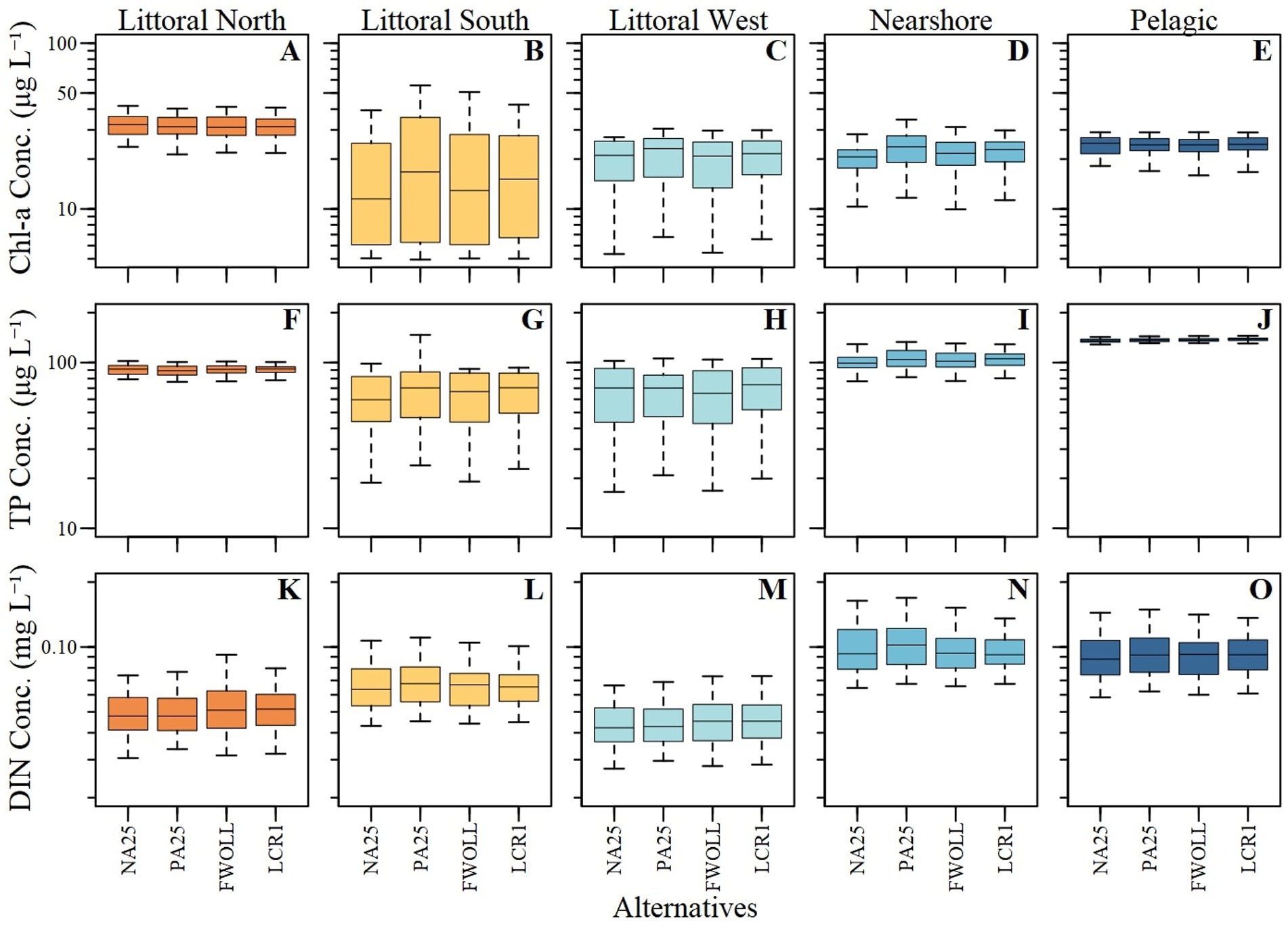
Figure 7. Boxplot of the 52-year period of simulation for each ecological zone predictions of chlorophyll-a concentration (A–E), total phosphorus (TP) concentrations (F–J), and dissolved inorganic nitrogen (DIN) concentrations (K–O) across Lake Okeechobee and alternatives.

Table 8

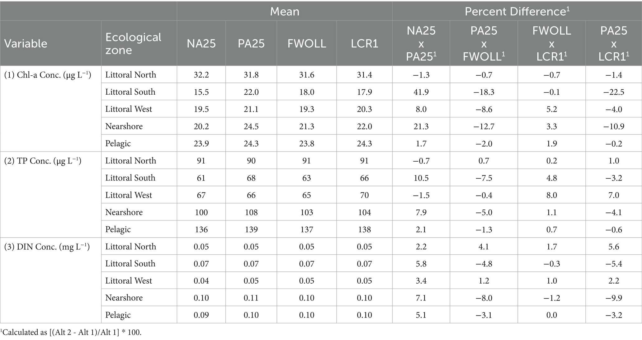
Table 8. Period of simulation mean and mean percent difference of predicted chlorophyll-a concentration (1), total phosphorus (TP) concentration (2), and dissolved inorganic nitrogen (DIN) concentration (3) across ecological zones and alternatives.

Discussion

Lake Okeechobee is a highly modified and heavily managed system with strong seasonal algal blooms that appear to be sensitive to water level management, as observed in this study and others (Havens, 1997, 2003). Additionally, while nutrient loading and concentrations have changed over time (Julian et al., 2023), internal nutrient loading has continued to subsidize the nutrient demand (Julian et al., In Prep), allowing for the proliferation of algal blooms. Watershed inputs, internal nutrient loading, and hydrodynamics have been identified as drivers of algal blooms for lakes that span the highly managed to semi-natural state (Havens et al., 2001; James et al., 2009; Isles et al., 2015).

Chlorophyll-a and phycocyanin concentrations within Lake Okeechobee follow a strong seasonal pattern that peaks during summer, when the days are relatively long with respect to daylight hours and temperatures (air and water) are warmer which corresponds to the start of the south Florida wet season (Figures 3B,F). Additionally, phycocyanin concentrations exhibit a dual peak seasonality suggesting something other than warm temperatures and long days contributed to the proliferation of the dominant pigment in cyanobacteria. While stage elevation has a significant effect on algal pigments (i.e., chlorophyll-a and phycocyanin), biogeochemical and hydrodynamic factors and processes also corresponded to changes in chlorophyll-a concentration over time with a notable spatial effect (Figures 2, 3D). However, due to spatial differences across the lake and how hydrodynamic and biogeochemical processes interacted across each ecological zone, stage alone was not sufficient enough to predict chlorophyll-a for all zones. Generally, littoral south, littoral west and nearshore zones are well characterized by changes in stage elevation (Figure 4). Although, including biogeochemical and hydrodynamic factors in a hierarchical statistical model framework provided a higher level of understanding concerning summer chlorophyll-a concentrations across ecological zones (Figure 7; Supplementary Table S4). The contrast between the hierarchical model and stage-based mixed models underscores the dynamic and complex drivers of phytoplankton in a highly variable system.

Seasonal patterns in algal biomass

Generally, in the northern hemisphere, algal biomass, expressed as chlorophyll-a concentrations, tends to peak between July and October (mid-summer to mid-fall) due to a complex interaction of between and within-season factors with significant intra- and inter-annual variability in peak season biomass (Singh and Singh, 2015; Wilkinson et al., 2022; Beal et al., 2023). This period was characterized by warmer temperatures and increased sunlight (longer days) that contributed to algal productivity. However, algal biomass is also driven by local hydrology and regional weather modulated to some degree by global climate teleconnections (weather and climate patterns that connect regions globally) (Beal et al., 2021). The hydrologic driver of algal productivity has been linked to the transport of external nutrients to lake ecosystems (Vollenweider, 1976; Schindler, 1977; Elliott et al., 2006) with watershed land cover composition influencing nutrient concentration and loading intensity (Bachmann et al., 2012; Xiong and Hoyer, 2019). Moreover, internal loading (nutrients fluxing from sediment and to some degree plant biomass decomposition) has resulted in a significant influence on the overlying water column and has been known to fuel algal blooms (Albright et al., 2022; Waters et al., 2023).

In addition to specific drivers of algae dynamics within discrete ecological zones, algae pigments varied spatially and temporally (Figure 3). While direct comparison of algal pigments (chlorophyll-a vs. phycocyanin) dynamics was problematic with the current analyses due to spatial and temporal limitations between datasets, it was apparent that stage elevation, season, and location affected pigment concentrations. Some drivers were different (e.g., seasonal and spatial; Figures 3B,F,D,H, respectively). Meanwhile, there appeared to be consistency with the influence of stage to some degree (Figures 3A,E; Supplementary Figure S2). The spatial differences observed in chlorophyll-a concentrations (Figure 3D) as demonstrated by the fine scale spatial effect, were consistent with zonal descriptions of algal dynamics in prior studies (Havens et al., 1994; Havens, 2003).

Lake Okeechobee experienced distinct wet and dry seasons where the wet season (May – October) corresponded with peak algal bloom periods. Moreover, the majority of surface water inputs occurred during the wet season. Wet season inputs combined with water management rules affected water storage volumes, water levels, and water retention times of the lake (Tarabih and Arias, 2021; Julian and Welch, 2022). Inflow discharges introduced the bulk of the surface water nutrient loads. However, internal lake loads were many times greater than surface water inputs (Havens and James, 2005) with some regions within the lake (i.e., pelagic) having a much higher sediment nutrient concentration, hence a nutrient reservoir (Julian et al., 2023). Internal loading effects on algal communities are not isolated to just Lake Okeechobee. In Lake Mendota (Wisconsin, United States), studies have demonstrated internal loading met phytoplankton demand for growth (Kamarainen et al., 2009b; Kamarainen et al., 2009a; Carpenter and Brock, 2024). This internal loading supplementation of phytoplankton simulation has been observed in other lake systems such as Lake Taihu (Ding et al., 2018; Yin et al., 2022), Lake Chaohu (Yang et al., 2020), Lake Rauwbraken (van Oosterhout et al., 2022), Lake Erie (Wang et al., 2021) to name a few.

Nearly all freshwater cyanobacteria contain phycocyanin, an accessory pigment that complements chlorophyll-a to produce energy, especially in low light conditions (Alegria Zufia et al., 2021; Kheimi et al., 2024). As observed in this study, chlorophyll-a and phycocyanin concentrations had distinct seasonality (Figure 3). This seasonal change corresponds with the typical algal biomass trends observed across the northern hemisphere in aquatic systems. However, phycocyanin concentrations within Lake Okeechobee exhibited a bimodal seasonality with the first peak occurring in the typical summer months followed by another peak later in the year (Figure 3). This bimodality was driven by either changes in light attenuation/water clarity, physiological changes in cyanobacteria due to changing seasonal conditions, shifts in species composition, or a combination of these factors (Zhang et al., 2016; Carpenter and Brock, 2024).

Seasonally, cyanobacteria blooms occurred in the summer months, predominately as Microcystis sp. (Supplementary Figure S3) between April to July. Meanwhile, later in the year between September and March there was a much more diverse cyanobacteria community composed of Microcystis sp., Cylindrospermopsis sp., Dolichopermum sp., and other species (Supplementary Figure S3). While phycocyanin pigments/sensors themselves cannot differentiate between species, they are more sensitive to detecting cyanobacteria specific biomass changes than just chlorophyll-a (Carpenter and Brock, 2024). However, in Lake Chaohu (Anhui Province, China), Zhang et al. (2016) observed seasonal changes in chlorophyll-a, phycocyanin concentrations, and species biomass. Additionally, Zhang et al. (2016) observed a bimodal seasonality in cyanobacteria biomass, with Anabaena sp. (now Dolichospermum sp.) as the dominant species contributing to this pattern, while Microcystis sp. was less dominant when bloom conditions peaked in summer and gradually declined throughout the rest of the year. While individual species demonstrated a single unimodal seasonality, together they exhibited a cyanobacteria biomass bimodal seasonality.

Algal bloom prediction

Generally, TP-chlorophyll-a statistical models have been used to predict chlorophyll-a concentrations, algal bloom conditions, and trophic conditions (Vollenweider, 1975, 1976; Nicholls and Dillon, 1978; Håkanson et al., 2005; Quinlan et al., 2021; Olson and Jones, 2022). However, these relationships typically had poor predictive capabilities due to stochastic dynamics, error, variability and uncertainty in predictors, simplified model structure and failure to meet model assumptions. Moreover, most of these models were developed using a single year or average values across several years thereby missing the year-to-year variability. Year-to-year variation in the TP-chlorophyll-a relationship has been significant, driven by a combination of internal and external processes that either maintain some disequilibrium or conflate inter-annual variation in relationships (Davidson et al., 2023). However, process-driven models, like the one presented by Olson and Jones (2022), can identify biological limitations and other factors driving variability in TP–chlorophyll-a relationships across space and time.

Between and within lakes the TP-chlorophyll-a relationship can be highly variable. Several synthesis studies have suggested the relationship was non-linear across the TP concentration continuum and affected by other factors. These factors included lake morphology, lake depth, thermal regime, N vs. P growth limitations, inputs, outflow, sedimentation, and depth-dependent processes (Guildford and Hecky, 2000; Phillips et al., 2008; Søndergaard et al., 2017; Qin et al., 2020; Quinlan et al., 2021; Davidson et al., 2023). Depth-dependent and hydrodynamic processes either directly affect the lake nutrient mass balance (e.g., changes in inflow P or N loads) or in-directly affect lake mixing, biotic interactions (e.g., zooplankton grazing) or biogeochemical cycling (e.g., denitrification). Some TP-chlorophyll-a modeling approaches attempted to account for the potential influences of these other factors by including lake depth, WRT, and water balance to name a few (Vollenweider, 1975; Olson and Jones, 2022).

Lake water depth, water level, or stage elevation, sometimes all used interchangeably, have been applied as metrics by water managers for reservoir and natural system management to estimate the storage volume in a given lake and to inform management decisions. Moreover, lake water level is a relatively easy and effective metric to measure. Storage volume, outflow discharge rate, and WRT are key factors in nutrient cycling, collectively influencing ‘contact time’—the duration for which nutrients remain available for uptake (dissolved) or settling (particulate).

Early Lake Okeechobee studies generally focused on algal biomass, TP concentrations, and water level (Walker and Havens, 1995; Havens and Walker, 2002). Prior studies documented a direct effect of water levels on algal biomass and recognized it as a local phenomenon generally restricted to the near-littoral region. However, on a lake-wide basis the correlation of stage and bloom frequency was observed to be highly variable (Havens et al., 1994; James et al., 1994). Lake Okeechobee is a spatially heterogeneous ecosystem with variability in physical attributes, water chemistry (Phlips et al., 1993), sediment nutrient distribution (Julian et al., 2023), and hydrodynamic influences (Chen and Sheng, 2003, 2005). These factors combined with seasonal variability in stage drives algal biomass trends and bloom frequency. This variability was also apparent in the stage-based chlorophyll-a and bloom frequency models developed by Walker (2020) and in this study (Figures 4, 6). Therefore, including other factors that account for the unique spatial characteristics of the system should provide a more robust estimation of algal biomass.

While phosphorus (P) is predominantly the limiting nutrient in most lake ecosystems, in some cases, nitrogen (N) can be a limiting nutrient for algal growth (Guildford and Hecky, 2000; Jones et al., 2008). Therefore, incorporating N into the TP-chlorophyll-a model can improve model fit and better explain changes in primary productivity (Søndergaard et al., 2017). While Lake Okeechobee has received high TP loads from its watershed, to the point of reducing its assimilative capacity and contributing to high internal loading (Havens and James, 2005; Julian et al., 2023) resulting in abundant resources for algal growth, N has been an important driver of algal dynamics as well.

For example, Havens (1995) documented a shift from P limitation to a secondary N limitation in the mid to late 1980s, however some variability in this limitation status has been identified across ecological regions of the lake (Supplementary Figure S4; Julian Unpublished Data). Moreover, it has been documented through in-situ observations and incubation experiments that algal dynamics in Lake Okeechobee have been driven in part by changes in DIN concentrations (Phlips and Ihnat, 1995; Gu et al., 1997; James et al., 2011). Based on this dynamic and the interplay between P, N, hydrodynamic characteristics, and the overall heterogeneity of the lake among regions, the hierarchical predictive models (i.e., LOK HABAM) presented in this study were developed to understand changes in chlorophyll-a with an aim to evaluate changes in system management. The inclusion of DIN and the interactive effect with TP allowed for capturing greater variability in the pelagic zone. In contrast, the stage-only model captured very little variability in the various algal bloom metrics with relatively flat slopes (Figure 4; Supplementary Table S3), resulting in reduced predictive capabilities in restoration scenarios (Figure 6). This result demonstrated that important ecosystem drivers other than stage influence this part of the system, consistent with prior studies discussed above.

Despite some variation in potential nutrient limitations (Supplementary Figure S4), prior studies have conducted nutrient limitation bioassays and determined that Lake Okeechobee is predominantly N-limiting, especially in summer when nitrate concentrations are typically the lowest (Supplementary Figure S5; Phlips and Ihnat, 1995; Philips et al., 1997; James et al., 2011). Additionally, Philips et al. (1997) noted regional occurrences of N and P co-limitation in the mid to late summer. These patterns suggest seasonal shifts in nutrient concentrations and biological cycling that align with variations in potential summer nutrient limitations observed over the period of record (Supplementary Figure S4). Meanwhile, ammonium concentrations remained relatively low and did not vary much between seasons (Supplementary Figure S5). Despite these low concentrations, Hampel et al. (2019) documented significant ammonium regeneration within Lake Okeechobee from internal sources suggesting rapid ammonium turnover rates have the ability to fuel and sustain algal blooms. Given this dynamic, including DIN concentrations as a predictor to the hierarchical predictive models not only resulted in an improved fit to the model it also captures the internal biogeochemical dynamics of the system.

Water management and planning

Water management, regional flood control, and restoration infrastructure (e.g., reservoirs, flow-equalization basins, stormwater treatment areas, etc.) have exhibited significant influences on local and regional hydrology as well as the ecology of lakes and downstream waterbodies (Havens, 2002; Richter et al., 2003; Julian and Welch, 2022). In the context of this study, both water management and restoration infrastructure were evaluated by comparing in-lake water, biogeochemical, and algal dynamics between LORS08 and LOSOM followed by the effect of utilizing storage north (LOCAR) and south (EAA Reservoir). Changes in lake hydrodynamics (i.e., inflow, outflow, storage volume, HRT, etc.) have shown a substantial effect on lake water quality and algal dynamics, effectively regulating the bioreactor nature of the lake as suggested by LOK HABAM and other modeling efforts in other lake ecosystems (Wang et al., 2013; Olson and Jones, 2022; Hanson et al., 2023).

As a potential application of LOK HABAM, water quality improvement scenarios were evaluated to understand the response of summer mean chlorophyll-a concentrations across the lake under LOSOM with the EAA reservoir in place. These scenarios are not necessarily the “how” but the final results of nutrient reductions observed within the lake. While more robust water quality modeling is needed, this modeling exercise demonstrates that not all parts of the lake respond similarly. Moreover, the predicted chlorophyll-a concentrations responded disproportionately with greater changes relative to in-lake TP concentration reductions (ranging from 10 to 30%) relative to concurrent changes in DIN concentrations (Supplementary Figure S6).

Under LOSOM (PA25) algal bloom conditions and/or bloom risk could be greater than all other alternatives. This risk is driven by significantly higher stage elevations relative to the baseline conditions (Julian and Welch, 2022) and alternatives associated with LOCAR (Figures 5–7) in its current eutrophic state with consistent exceedance of the regulatory inflow load limit. Although with the addition of southern storage features (FWOLL) and the addition of northern storage (LCR1) with LOSOM in place, the benefits of LOSOM (i.e., reduce discharges to northern Estuaries, increased discharges to the Everglades) (Julian and Reidenbach, 2024) were achieved and algal bloom risk was reduced with added storage. This added storage aids in modulating water levels in the lake by buffering high flow events from the north and reducing periods of high-water levels thereby improving the lake’s ecology and building resilience in the system (Figure 5). The combined effect of water management utilizing the necessary storage infrastructure significantly improved the hydrodynamic condition of the lake, which can alleviate some ecological stress associated with high water levels (Julian and Welch, 2022). However, other issues remained that also contribute to the lake’s chronic algal bloom and eutrophic condition, including high nutrient inflow loads and the legacy effect of high nutrient storage in lake sediment. While an attempt was made to address inflow nutrient loads with water quality improvement projects and deployment of best management practices, efforts may need to be more aggressive to achieve the expected goal outlined in the Lake Okeechobee Basin Action Management Plan to ensure that the Total Maximum Daily Load can be achieved (Florida Department of Environmental Protection, 2020; Julian et al., 2023).

Data availability statement

Publicly available datasets were analyzed in this study. This data can be found here: Data used in this study is publicly available from the South Florida Water Management District, DBHYDRO (https://www.sfwmd.gov/dbhydro), and Statewide Model Management System (https://apps.sfwmd.gov/smmsviewer/). R scripts used to analyze these data are also available on Github (https://github.com/SwampThingPaul/LOK_AlgaeEval_manu).

Author contributions

PJ: Validation, Methodology, Visualization, Data curation, Formal analysis, Software, Conceptualization, Writing – original draft, Writing – review & editing. WW: Writing – review & editing, Conceptualization. DS: Writing – review & editing, Writing – original draft, Conceptualization. SD: Writing – review & editing, Conceptualization, Writing – original draft.

Funding

The author(s) declare that no financial support was received for the research and/or publication of this article.

Acknowledgments

The authors would like to thank the US Army Corps of Engineers and the South Florida Water Management District for making the modeling output available. The authors would also like to thank the peer reviewer(s) and editor(s) for their efforts and constructive review of this manuscript.

Conflict of interest

PJ and SD were employed by The Everglades Foundation.

The remaining authors declare that the research was conducted in the absence of any commercial or financial relationships that could be construed as a potential conflict of interest.

Generative AI statement

The authors declare that no Gen AI was used in the creation of this manuscript.

Publisher’s note

All claims expressed in this article are solely those of the authors and do not necessarily represent those of their affiliated organizations, or those of the publisher, the editors and the reviewers. Any product that may be evaluated in this article, or claim that may be made by its manufacturer, is not guaranteed or endorsed by the publisher.

Supplementary material

The Supplementary material for this article can be found online at: https://www.frontiersin.org/articles/10.3389/frwa.2025.1619838/full#supplementary-material

Footnotes

1. ^https://swampthingpaul.shinyapps.io/lok_algaeevaltool/

2. ^https://github.com/SwampThingPaul/LOK_AlgaeEval

References

Albright, E. A., Rachel, F. K., Shingai, Q. K., and Wilkinson, G. M. (2022). High inter- and intra-lake variation in sediment phosphorus pools in shallow lakes. J. Geophys. Res. Biogeosci. 127:e2022JG006817. doi: 10.1029/2022JG006817

Crossref Full Text | Google Scholar

Alegria Zufia, J., Farnelid, H., and Legrand, C. (2021). Seasonality of coastal Picophytoplankton growth, nutrient limitation, and biomass contribution. Front. Microbiol. 12:590. doi: 10.3389/fmicb.2021.786590

PubMed Abstract | Crossref Full Text | Google Scholar

Anderson, T. W., and Darling, D. A. (1952). Asymptotic theory of certain “goodness of fit” criteria based on stochastic processes. Ann. Math. Stat. 23, 193–212. doi: 10.1214/aoms/1177729437

Crossref Full Text | Google Scholar

Aumen, N. G. (1995). “The history of human impacts, lake management, and limnological research on Lake Okeechobee, Florida (USA)” in Advances in limnology. eds. N. G. Aumen and R. G. Wetzel (Stuttgart: Germany).

Google Scholar

Bachmann, R. W., Bigham, D. L., Hoyer, M. V., and Canfield, D. E. (2012). A strategy for establishing numeric nutrient criteria for Florida lakes. Lake Reserv. Manage. 28, 84–91. doi: 10.1080/07438141.2012.667053

Crossref Full Text | Google Scholar

Backer, L. C. (2002). Cyanobacterial harmful algal blooms (CyanoHABs): developing a public health response. Lake Reserv. Manage. 18, 20–31. doi: 10.1080/07438140209353926

Crossref Full Text | Google Scholar

Beal, M. R. W., O’Reilly, B., Hietpas, K. R., and Block, P. (2021). Development of a sub-seasonal cyanobacteria prediction model by leveraging local and global scale predictors. Harmful Algae 108:102100. doi: 10.1016/j.hal.2021.102100

Crossref Full Text | Google Scholar

Beal, M. R. W., Wilkinson, G. M., and Block, P. J. (2023). Large scale seasonal forecasting of peak season algae metrics in the Midwest and northeast U.S. Water Res. 229:119402. doi: 10.1016/j.watres.2022.119402

PubMed Abstract | Crossref Full Text | Google Scholar

Bras, R. L., Ponce, V. M., and Sheer, D. (2019). Peer review of the regional simulation model. West Palm Beach, FL: South Florida water Management District.

Google Scholar

Carmichael, W. W. (2001). Health effects of toxin-producing Cyanobacteria: “the CyanoHABs.”. Hum. Ecol. Risk. Assess. 7, 1393–1407. doi: 10.1080/20018091095087

Crossref Full Text | Google Scholar

Carpenter, S. R., and Brock, W. A. (2024). Stochastic dynamics of phycocyanin in years of contrasting phosphorus load. Ecosphere 15:e4903. doi: 10.1002/ecs2.4903

Crossref Full Text | Google Scholar

Chen, X., and Sheng, Y. P. (2003). Modeling phosphorus dynamics in a shallow lake during an episodic event. Lake Reserv. Manage. 19, 323–340. doi: 10.1080/07438140309353942

Crossref Full Text | Google Scholar

Chen, X., and Sheng, Y. P. (2005). Three-dimensional modeling of sediment and phosphorus dynamics in Lake Okeechobee, Florida: spring 1989 simulation. J. Environ. Eng. 131, 359–374. doi: 10.1061/(ASCE)0733-9372(2005)131:3(359)

Crossref Full Text | Google Scholar

Chin, D. A., Dracup, J. A., Jones, N. L., Ponce, V. M., Schaffranek, R. W., and Therrien, R. (2005). Peer review of the regional simulation model. West Palm Beach, FL: South Florida Water Management District.

Google Scholar

Chorus, I., and Welker, M. (2021). Toxic cyanobacteria in water: A guide to their public health consequences, monitoring and management. 2nd Edn. Boca Raton, FL: CRC Press.

Google Scholar

Cichra, M. F., Badylak, S., Henderson, N., Rueter, B. H., and Phlips, E. J. (1995). Phytoplankton community structure in the open water zone of a shallow subtropical lake (Lake Okeechobee, Florida, USA). Ergeb. Limnol. 1, 157–176.

Google Scholar

Davidson, T. A., Sayer, C. D., Jeppesen, E., Søndergaard, M., Lauridsen, T. L., Johansson, L. S., et al. (2023). Bimodality and alternative equilibria do not help explain long-term patterns in shallow lake chlorophyll-a. Nat. Commun. 14:398. doi: 10.1038/s41467-023-36043-9

PubMed Abstract | Crossref Full Text | Google Scholar

Ding, S., Chen, M., Gong, M., Fan, X., Qin, B., Xu, H., et al. (2018). Internal phosphorus loading from sediments causes seasonal nitrogen limitation for harmful algal blooms. Sci. Total Environ. 625, 872–884. doi: 10.1016/j.scitotenv.2017.12.348

PubMed Abstract | Crossref Full Text | Google Scholar

Elliott, J. A., Jones, I. D., and Thackeray, S. J. (2006). Testing the sensitivity of phytoplankton communities to changes in water temperature and nutrient load, in a temperate lake. Hydrobiologia 559, 401–411. doi: 10.1007/s10750-005-1233-y

Crossref Full Text | Google Scholar

Elser, J. J., Bracken, M. E. S., Cleland, E. E., Gruner, D. S., Harpole, W. S., Hillebrand, H., et al. (2007). Global analysis of nitrogen and phosphorus limitation of primary producers in freshwater, marine and terrestrial ecosystems. Ecol. Lett. 10, 1135–1142. doi: 10.1111/j.1461-0248.2007.01113.x

PubMed Abstract | Crossref Full Text | Google Scholar

Engstrom, D. R., Schottler, S. P., Leavitt, P. R., and Havens, K. E. (2006). A reevaluation of the cultural eutrophication of Lake Okeechobee using multiproxy sediment records. Ecol. Appl. 16, 1194–1206. doi: 10.1890/1051-0761(2006)016[1194:arotce]2.0.co;2

PubMed Abstract | Crossref Full Text | Google Scholar

Faith, D. P., Minchin, P. R., and Belbin, L. (1987). Compositional dissimilarity as a robust measure of ecological distance. Vegetatio 69, 57–68. doi: 10.1007/BF00038687

Crossref Full Text | Google Scholar

Fisher, M. M., Reddy, K. R., and James, R. T. (2001). Long-term changes in the sediment chemistry of a large shallow subtropical lake. Lake Reserv. Manage. 17, 217–232. doi: 10.1080/07438140109354132

Crossref Full Text | Google Scholar

Florida Administrative Code (2016a). Chapter 62–302. 531 numeric interpretation of NArrative nutrient criteria. Florida: Florida Administrative Code.

Google Scholar

Florida Administrative Code (2016b). Chapter 62–303 identification of impaired surface Waters. Florida: Florida Administrative Code.

Google Scholar

Florida Department of Environmental Protection (2020). Lake Okeechobee basin management action plan. Tallahassee, FL: Florida Department of Environmental Protection.

Google Scholar

Gu, B., Havens, K. E., Schelske, C. L., and Rosen, B. H. (1997). Uptake of dissolved nitrogen by phytoplankton in a eutrophic subtropical lake. J. Plankton Res. 19, 759–770. doi: 10.1093/plankt/19.6.759

Crossref Full Text | Google Scholar

Guildford, S. J., and Hecky, R. E. (2000). Total nitrogen, total phosphorus, and nutrient limitation in lakes and oceans: is there a common relationship? Limnol. Oceanogr. 45, 1213–1223. doi: 10.4319/lo.2000.45.6.1213

Crossref Full Text | Google Scholar

Gupta, H. V., Kling, H., Yilmaz, K. K., and Martinez, G. F. (2009). Decomposition of the mean squared error and NSE performance criteria: implications for improving hydrological modelling. J. Hydrol. 377, 80–91. doi: 10.1016/j.jhydrol.2009.08.003

Crossref Full Text | Google Scholar

Håkanson, L., Blenckner, T., Bryhn, A. C., and Hellström, S.-S. (2005). The influence of calcium on the chlorophyll–phosphorus relationship and lake Secchi depths. Hydrobiologia 537, 111–123. doi: 10.1007/s10750-004-2605-4

Crossref Full Text | Google Scholar

Hampel, J. J., McCarthy, M. J., Reed, M. H., and Newell, S. E. (2019). Short term effects of hurricane Irma and cyanobacterial blooms on ammonium cycling along a freshwater–estuarine continuum in South Florida. Front. Mar. Sci. 6:640. doi: 10.3389/fmars.2019.00640

Crossref Full Text | Google Scholar

Hanson, P. C., Ladwig, R., Buelo, C., Albright, E. A., Delany, A. D., and Carey, C. C. (2023). Legacy phosphorus and ecosystem memory control future water quality in a eutrophic lake. J. Geophys. Res. Biogeosci. 128:e2023JG007620. doi: 10.1029/2023JG007620

Crossref Full Text | Google Scholar

Harris, W. G., Fisher, M. M., Cao, X., Osborne, T., and Ellis, L. (2007). Magnesium-rich minerals in sediment and suspended particulates of South Florida water bodies: implications for turbidity. J. Environ. Qual. 36, 1670–1677. doi: 10.2134/jeq2006.0559

PubMed Abstract | Crossref Full Text | Google Scholar

Havens, K. E. (1994). Relationships of annual chlorophyll a means, maxima, and algal bloom frequencies in a shallow eutrophic lake (Lake Okeechobee, Florida, USA). Lake Reserv. Manage. 10, 133–136. doi: 10.1080/07438149409354184

Crossref Full Text | Google Scholar

Havens, K. E. (1995). Secondary nitrogen limitation in a subtropical lake impacted by non-point source agricultural pollution. Environ. Pollut. 89, 241–246. doi: 10.1016/0269-7491(94)00076-P

PubMed Abstract | Crossref Full Text | Google Scholar

Havens, K. E. (1997). Water levels and total phosphorus in Lake Okeechobee. Lake Reserv. Manage. 13, 16–25. doi: 10.1080/07438149709354292

Crossref Full Text | Google Scholar

Havens, K. E. (2002). Development and application of hydrologic restoration goals for a large subtropical lake. Lake Reserv. Manage. 18, 285–292. doi: 10.1080/07438140209353934

Crossref Full Text | Google Scholar

Havens, K. E. (2003). Phosphorus–algal bloom relationships in large lakes of South Florida: implications for establishing nutrient criteria. Lake Reserv. Manage. 19, 222–228. doi: 10.1080/07438140309354087

Crossref Full Text | Google Scholar

Havens, K. E., Fukushima, T., Xie, P., Iwakuma, T., James, R. T., Takamura, N., et al. (2001). Nutrient dynamics and the eutrophication of shallow lakes Kasumigaura (Japan), Donghu (PR China), and Okeechobee (USA). Environ. Pollut. 111, 263–272. doi: 10.1016/S0269-7491(00)00074-9

PubMed Abstract | Crossref Full Text | Google Scholar

Havens, K. E., Hanlon, C., and James, R. T. (1994). Seasonal and spatial variation in algal bloom frequencies in Lake Okeechobee, Florida, U.S.a. Lake Reserv. Manage. 10, 139–148. doi: 10.1080/07438149409354185

Crossref Full Text | Google Scholar

Havens, K. E., Hanlon, C., and James, R. T. (1995). Historical trends in the Lake Okeechobee ecosystem. V. Algal blooms. Arch. Hydrobiol. 1, 89–100.

Google Scholar

Havens, K. E., and James, R. T. (2005). The phosphorus mass balance of Lake Okeechobee, Florida: implications for eutrophication management. Lake Reserv. Manage. 21, 139–148. doi: 10.1080/07438140509354423

Crossref Full Text | Google Scholar

Havens, K., Paerl, H., Phlips, E., Zhu, M., Beaver, J., and Srifa, A. (2016). Extreme weather events and climate variability provide a lens to how shallow lakes may respond to climate change. Water 8:229. doi: 10.3390/w8060229

Crossref Full Text | Google Scholar

Havens, K. E., and Walker, W. W. (2002). Development of a total phosphorus concentration goal in the TMDL process for Lake Okeechobee, Florida (USA). Lake Reserv. Manag. 18, 227–238. doi: 10.1080/07438140209354151

Crossref Full Text | Google Scholar

Isles, P. D. F., Giles, C. D., Gearhart, T. A., Xu, Y., Druschel, G. K., and Schroth, A. W. (2015). Dynamic internal drivers of a historically severe cyanobacteria bloom in Lake Champlain revealed through comprehensive monitoring. J. Great Lakes Res. 41, 818–829. doi: 10.1016/j.jglr.2015.06.006

Crossref Full Text | Google Scholar

James, R. T., Gardner, W. S., McCarthy, M. J., and Carini, S. A. (2011). Nitrogen dynamics in Lake Okeechobee: forms, functions, and changes. Hydrobiologia 669, 199–212. doi: 10.1007/s10750-011-0683-7

Crossref Full Text | Google Scholar

James, R. T., Havens, K., Zhu, G., and Qin, B. (2009). Comparative analysis of nutrients, chlorophyll and transparency in two large shallow lakes (Lake Taihu, P.R. China and Lake Okeechobee, USA). Hydrobiologia 627, 211–231. doi: 10.1007/s10750-009-9729-5

Crossref Full Text | Google Scholar

James, R. T., Smith, V., and Jones, B. L. (1994). Historical trends in the Lake Okeechobee ecosystem. III. Water quality. Arch. Hydrobiol. 107, 49–69.

Google Scholar

Jones, J. R., Obrecht, D. V., Perkins, B. D., Knowlton, M. F., Thorpe, A. P., Watanabe, S., et al. (2008). Nutrients, seston, and transparency of Missouri reservoirs and oxbow lakes: an analysis of regional limnology. Lake Reserv. Manage. 24, 155–180. doi: 10.1080/07438140809354058

Crossref Full Text | Google Scholar

Julian, P., and Reidenbach, L. (2024). Upstream water management and its role in estuary health, evaluation of freshwater management and subtropical estuary function. Watershed Ecol. Environ. 6, 84–94. doi: 10.1016/j.wsee.2024.05.002

Crossref Full Text | Google Scholar

Julian, P., Schafer, T., Cohen, M. J., Jones, P., and Osborne, T. Z. (2023). Changes in the spatial distribution of total phosphorus in sediment and water column of a shallow subtropical lake. Lake Reserv. Manage. 39, 213–230. doi: 10.1080/10402381.2023.2243606

Crossref Full Text | Google Scholar

Julian, P., Thompson, M., and Milbrandt, E. C. (2024). Dark waters: evaluating seagrass community response to optical water quality and freshwater discharges in a highly managed subtropical estuary. Reg. Stud. Mar. Sci. 69:103302. doi: 10.1016/j.rsma.2023.103302

Crossref Full Text | Google Scholar

Julian, P., and Welch, Z. (2022). Understanding the ups and downs, application of hydrologic restoration measures for a large subtropical lake. Lake Reserv. Manage. 38, 304–317. doi: 10.1080/10402381.2022.2126806

Crossref Full Text | Google Scholar

Kamarainen, A. M., Penczykowski, R. M., Van de Bogert, M. C., Hanson, P. C., and Carpenter, S. R. (2009a). Phosphorus sources and demand during summer in a eutrophic lake. Aquat. Sci. 71, 214–227. doi: 10.1007/s00027-009-9165-7

Crossref Full Text | Google Scholar

Kamarainen, A. M., Yuan, H., Wu, C. H., and Carpenter, S. R. (2009b). Estimates of phosphorus entrainment in Lake Mendota: a comparison of one-dimensional and three-dimensional approaches. Limnol. Oceanogr. Methods 7, 553–567. doi: 10.4319/lom.2009.7.553

Crossref Full Text | Google Scholar

Kheimi, M., Almadani, M., Ramezani-Charmahineh, A., and Zounemat-Kermani, M. (2024). Study of biological quality of lake waters based on phycocyanin using tree-based methodologies. Ecohydrology 17:e2688. doi: 10.1002/eco.2688

Crossref Full Text | Google Scholar

Lefler, F. W., Barbosa, M., Zimba, P. V., Smyth, A. R., Berthold, D. E., and Laughinghouse, H. D. (2023). Spatiotemporal diversity and community structure of cyanobacteria and associated bacteria in the large shallow subtropical Lake Okeechobee (Florida, United States). Front. Microbiol. 14:261. doi: 10.3389/fmicb.2023.1219261

PubMed Abstract | Crossref Full Text | Google Scholar

Macário, I. P., Castro, B. B., Nunes, M. I., Antunes, S. C., Pizarro, C., Coelho, C., et al. (2015). New insights towards the establishment of phycocyanin concentration thresholds considering species-specific variability of bloom-forming cyanobacteria. Hydrobiologia 757, 155–165. doi: 10.1007/s10750-015-2248-7

Crossref Full Text | Google Scholar

MacKeigan, P. W., Taranu, Z. E., Pick, F. R., Beisner, B. E., and Gregory-Eaves, I. (2023). Both biotic and abiotic predictors explain significant variation in cyanobacteria biomass across lakes from temperate to subarctic zones. Limnol. Oceanogr. 68, 1360–1375. doi: 10.1002/lno.12352

Crossref Full Text | Google Scholar

Marshall, M. L. (1977). Phytoplankton and primary productivity studies in Lake Okeechobee during 1974. West Palm Beach, FL: South Florida Water Management District.

Google Scholar

Martinsen, K. T., and Sand-Jensen, K. (2022). Predicting water quality from geospatial lake, catchment, and buffer zone characteristics in temperate lowland lakes. Sci. Total Environ. 851:158090. doi: 10.1016/j.scitotenv.2022.158090

PubMed Abstract | Crossref Full Text | Google Scholar

Matthews, M. W. (2011). A current review of empirical procedures of remote sensing in inland and near-coastal transitional waters. Int. J. Remote Sens. 32, 6855–6899. doi: 10.1080/01431161.2010.512947

Crossref Full Text | Google Scholar

Mowe, M. A. D., Porojan, C., Abbas, F., Mitrovic, S. M., Lim, R. P., Furey, A., et al. (2015). Rising temperatures may increase growth rates and microcystin production in tropical Microcystis species. Harmful Algae 50, 88–98. doi: 10.1016/j.hal.2015.10.011

Crossref Full Text | Google Scholar

Nicholls, K. H., and Dillon, P. J. (1978). An evaluation of phosphorus-chlorophyll-phytoplankton relationships for lakes. Int. Rev. Gesamten Hydrobiol. 63, 141–154. doi: 10.1002/iroh.19780630203

Crossref Full Text | Google Scholar

O’Neil, J. M., Davis, T. W., Burford, M. A., and Gobler, C. J. (2012). The rise of harmful cyanobacteria blooms: the potential roles of eutrophication and climate change. Harmful Algae 14, 313–334. doi: 10.1016/j.hal.2011.10.027

Crossref Full Text | Google Scholar

Oksanen, J., and Guillaume, F. (2018). Vegan: Ecological diversity. CRAN R-project.

Google Scholar

Olson, C. R., and Jones, S. E. (2022). Chlorophyll–total phosphorus relationships emerge from multiscale interactions from algae to catchments. Limnol. Oceanogr. Lett. 7:10281. doi: 10.1002/lol2.10281

Crossref Full Text | Google Scholar

Orihel, D. M., Bird, D. F., Brylinsky, M., Chen, H., Donald, D. B., Huang, D. Y., et al. (2012). High microcystin concentrations occur only at low nitrogen-to-phosphorus ratios in nutrient-rich Canadian lakes. Can. J. Fish. Aquat. Sci. 69, 1457–1462. doi: 10.1139/f2012-088

Crossref Full Text | Google Scholar

Painter, K. J., Venkiteswaran, J. J., and Baulch, H. M. (2023). Blooms and flows: effects of variable hydrology and management on reservoir water quality. Ecosphere 14:e4472. doi: 10.1002/ecs2.4472

Crossref Full Text | Google Scholar

Pedersen, E. J., Miller, D. L., Simpson, G. L., and Ross, N. (2019). Hierarchical generalized additive models in ecology: an introduction with mgcv. PeerJ 7:e6876. doi: 10.7717/peerj.6876

PubMed Abstract | Crossref Full Text | Google Scholar

Pettitt, A. N. (1976). A two-sample Anderson-Darling rank statistic. Biometrika 63, 161–168. doi: 10.1093/biomet/63.1.161

Crossref Full Text | Google Scholar

Philips, E. J., Cichra, M., Havens, K., Hanton, C., Badylak, S., Rueter, B., et al. (1997). Relationships between phytoplankton dynamics and the availability of light and nutrients in a shallow sub-tropical lake. J. Plankton Res. 19, 319–342. doi: 10.1093/plankt/19.3.319

Crossref Full Text | Google Scholar

Phillips, G., Pietiläinen, O.-P., Carvalho, L., Solimini, A., Lyche Solheim, A., and Cardoso, A. C. (2008). Chlorophyll–nutrient relationships of different lake types using a large European dataset. Aquat. Ecol. 42, 213–226. doi: 10.1007/s10452-008-9180-0

Crossref Full Text | Google Scholar

Phlips, E. J., Aldridge, F. J., Hansen, P., Zimba, P. V., Ihnat, J., Conroy, M., et al. (1993). Spatial and temporal variability of trophic state parameters in a shallow subtropical lake (Lake Okeechobee, Florida, USA). Archiv_Hydrobiol. 128, 437–458. doi: 10.1127/archiv-hydrobiol/128/1993/437

Crossref Full Text | Google Scholar

Phlips, E., and Ihnat, J. (1995). Planktonic nitrogen fixation in a shallow subtropical lake (Lake Okeechobee, Florida, USA). Adv. Limnol. 45, 191–201.

Google Scholar

Qin, B., Zhou, J., Elser, J. J., Gardner, W. S., Deng, J., and Brookes, J. D. (2020). Water depth underpins the relative roles and fates of nitrogen and phosphorus in lakes. Environ. Sci. Technol. 54, 3191–3198. doi: 10.1021/acs.est.9b05858

PubMed Abstract | Crossref Full Text | Google Scholar

Qiu, C., and Wan, Y. (2013). Time series modeling and prediction of salinity in the Caloosahatchee River estuary. Water Resour. Res. 49, 5804–5816. doi: 10.1002/wrcr.20415

Crossref Full Text | Google Scholar

Quinlan, R., Filazzola, A., Mahdiyan, O., Shuvo, A., Blagrave, K., Ewins, C., et al. (2021). Relationships of total phosphorus and chlorophyll in lakes worldwide. Limnol. Oceanogr. 66, 392–404. doi: 10.1002/lno.11611

Crossref Full Text | Google Scholar

Richter, B. D., Mathews, R., Harrison, D. L., and Wigington, R. (2003). Ecologically sustainable water management: managing river flows for ecological integrity. Ecol. Appl. 13, 206–224. doi: 10.1890/1051-0761(2003)013[0206:ESWMMR]2.0.CO;2

Crossref Full Text | Google Scholar

Rousso, B. Z., Bertone, E., Stewart, R., Aguiar, A., Chuang, A., Hamilton, D. P., et al. (2022). Chlorophyll and phycocyanin in-situ fluorescence in mixed cyanobacterial species assemblages: effects of morphology, cell size and growth phase. Water Res. 212:118127. doi: 10.1016/j.watres.2022.118127

PubMed Abstract | Crossref Full Text | Google Scholar

Saros, J. E., Hazuková, V., Northington, R. M., Huston, G. P., Lamb, A., Birkel, S., et al. (2025). Abrupt transformation of West Greenland lakes following compound climate extremes associated with atmospheric rivers. Proc. Natl. Acad. Sci. 122:e2413855122. doi: 10.1073/pnas.2413855122

PubMed Abstract | Crossref Full Text | Google Scholar

Schindler, D. W. (1977). Evolution of phosphorus limitation in lakes. Science 195, 260–262. doi: 10.1126/science.195.4275.260

PubMed Abstract | Crossref Full Text | Google Scholar

Schindler, D. W., Hecky, R. E., Findlay, D. L., Stainton, M. P., Parker, B. R., Paterson, M. J., et al. (2008). Eutrophication of lakes cannot be controlled by reducing nitrogen input: results of a 37-year whole-ecosystem experiment. Proc. Natl. Acad. Sci. 105, 11254–11258. doi: 10.1073/pnas.0805108105

PubMed Abstract | Crossref Full Text | Google Scholar

Scholz, F., and Zhu, A. (2023). kSamples: K-sample rank tests and their combinations. CRAN R-project.

Google Scholar

Simpson, G. L. (2018). Modelling palaeoecological time series using generalised additive models. Front. Ecol. Evol. 6:149. doi: 10.3389/fevo.2018.00149

Crossref Full Text | Google Scholar

Simpson, G. L. (2021). Gratia: Graceful ‘ggplot’-based graphics and other functions for GAMS fitted using “mcgv”. CRAN R-Project. Available at: https://gavinsimpson.github.io/gratia/.

Google Scholar

Singh, S. P., and Singh, P. (2015). Effect of temperature and light on the growth of algae species: a review. Renew. Sust. Energ. Rev. 50, 431–444. doi: 10.1016/j.rser.2015.05.024

Crossref Full Text | Google Scholar

Søndergaard, M., Lauridsen, T. L., Johansson, L. S., and Jeppesen, E. (2017). Nitrogen or phosphorus limitation in lakes and its impact on phytoplankton biomass and submerged macrophyte cover. Hydrobiologia 795, 35–48. doi: 10.1007/s10750-017-3110-x

Crossref Full Text | Google Scholar

Song, K., and Burgin, A. J. (2017). Perpetual phosphorus cycling: eutrophication amplifies biological control on internal phosphorus loading in agricultural reservoirs. Ecosystems 20, 1483–1493. doi: 10.1007/s10021-017-0126-z

Crossref Full Text | Google Scholar

South Florida Water Management District (2020). Technical document to support the Central Everglades planning project: Everglades agricultural area reservoir water reservation. West Palm Beach, FL: South Florida Water Management District.

Google Scholar

Stumpf, R. P., Davis, T. W., Wynne, T. T., Graham, J. L., Loftin, K. A., Johengen, T. H., et al. (2016). Challenges for mapping cyanotoxin patterns from remote sensing of cyanobacteria. Harmful Algae 54, 160–173. doi: 10.1016/j.hal.2016.01.005

PubMed Abstract | Crossref Full Text | Google Scholar

Tarabih, O. M., and Arias, M. E. (2021). Hydrological and water quality trends through the lens of historical operation schedules in Lake Okeechobee. J. Water Resour. Plan. Manag. 147:04021034. doi: 10.1061/(ASCE)WR.1943-5452.0001395

Crossref Full Text | Google Scholar

Thomson-Laing, G., Puddick, J., and Wood, S. A. (2020). Predicting cyanobacterial biovolumes from phycocyanin fluorescence using a handheld fluorometer in the field. Harmful Algae 97:101869. doi: 10.1016/j.hal.2020.101869

PubMed Abstract | Crossref Full Text | Google Scholar

US Army Corps of Engineers (2024a). Final environmental impact statement: Lake Okeechobee system operating manual. Jacksonville, FL: US Army Corp of Engineers.

Google Scholar

US Army Corps of Engineers (2024b). Final environmental impact statement: North of Lake Okeechobee storage reservoir section 203 study. Jacksonville, FL: US Army Corp of Engineers.

Google Scholar

USACE (2024). Final environmental impact statement: North of Lake Okeechobee storage reservoir - section 203 study. Jacksonville, FL: US Army Corp of Engineers.

Google Scholar

van Oosterhout, F., Yasseri, S., Noyma, N., Huszar, V., Manzi Marinho, M., Mucci, M., et al. (2022). Assessing the long-term efficacy of internal loading management to control eutrophication in Lake Rauwbraken. Inland Waters 12, 61–77. doi: 10.1080/20442041.2021.1969189

Crossref Full Text | Google Scholar

Vollenweider, R. A. (1975). Input-output models: with special reference to the phosphorus loading concept in limnology. Schweiz. Z. Hydrol. 37, 53–84. doi: 10.1007/BF02505178

Crossref Full Text | Google Scholar

Vollenweider, R. A. (1976). Advances in defining critical loading levels for phosphorus in lake eutrophication. Mem. Ist. Ital. Idrobiol. 33, 53–58.

Google Scholar

Walker, W. W. (2020). Draft - chlorophyll-a models for LOSOM applications. Department of Interior.

Google Scholar

Walker, W. W., and Havens, K. E. (1995). Relating algal bloom frequencies to phosphorus concentrations in Lake Okeechobee. Lake Reserv. Manage. 11, 77–83. doi: 10.1080/07438149509354200

Crossref Full Text | Google Scholar

Wang, F., Wang, X., Chen, B., Zhao, Y., and Yang, Z. (2013). Chlorophyll a simulation in a Lake ecosystem using a model with wavelet analysis and artificial neural network. Environ. Manag. 51, 1044–1054. doi: 10.1007/s00267-013-0029-5

PubMed Abstract | Crossref Full Text | Google Scholar

Wang, Y. T., Zhang, T. Q., Zhao, Y. C., Ciborowski, J. J. H., Zhao, Y. M., O’Halloran, I. P., et al. (2021). Characterization of sedimentary phosphorus in Lake Erie and on-site quantification of internal phosphorus loading. Water Res. 188:116525. doi: 10.1016/j.watres.2020.116525

Crossref Full Text | Google Scholar

Waters, S., Atalah, J., Thompson, L., Thomson-Laing, G., Pearman, J. K., Puddick, J., et al. (2023). It’s all in the mud - the use of sediment geochemistry to estimate contemporary water quality in lakes. Appl. Geochem. 153:105667. doi: 10.1016/j.apgeochem.2023.105667

Crossref Full Text | Google Scholar

Wilkinson, G. M., Walter, J. A., Buelo, C. D., and Pace, M. L. (2022). No evidence of widespread algal bloom intensification in hundreds of lakes. Front. Ecol. Environ. 20, 16–21. doi: 10.1002/fee.2421

Crossref Full Text | Google Scholar

Wood, S. N. (2017). Generalized additive models: An introduction with R. 2nd Edn. Boca Raton, FL: CRC Press.

Google Scholar

Wu, Z., Li, J., Sun, Y., Peñuelas, J., Huang, J., Sardans, J., et al. (2022). Imbalance of global nutrient cycles exacerbated by the greater retention of phosphorus over nitrogen in lakes. Nat. Geosci. 15, 464–468. doi: 10.1038/s41561-022-00958-7

Crossref Full Text | Google Scholar

Xiong, C., and Hoyer, M. V. (2019). Influence of land use and rainfall variability on nutrient concentrations in Florida lakes. Lake Reserv. Manage. 35, 25–37. doi: 10.1080/10402381.2018.1511659

Crossref Full Text | Google Scholar

Yang, C., Yang, P., Geng, J., Yin, H., and Chen, K. (2020). Sediment internal nutrient loading in the most polluted area of a shallow eutrophic lake (Lake Chaohu, China) and its contribution to lake eutrophication. Environ. Pollut. 262:114292. doi: 10.1016/j.envpol.2020.114292

PubMed Abstract | Crossref Full Text | Google Scholar

Yin, H., Zhang, M., Yin, P., and Li, J. (2022). Characterization of internal phosphorus loading in the sediment of a large eutrophic Lake (lake Taihu, China). Water Res. 225:119125. doi: 10.1016/j.watres.2022.119125

PubMed Abstract | Crossref Full Text | Google Scholar

Zhang, M., Zhang, Y., Yang, Z., Wei, L., Yang, W., Chen, C., et al. (2016). Spatial and seasonal shifts in bloom-forming cyanobacteria in Lake Chaohu: patterns and driving factors. Phycol. Res. 64, 44–55. doi: 10.1111/pre.12112

Crossref Full Text | Google Scholar