From Epidemic to Pandemic Modelling

1 Introduction

We present a methodology for modelling pandemics, the development of which was motivated by the current COVID19 outbreak. The key point of our approach is the introduction of geography and travel connections in a well founded manner, facilitating intuitive understanding by modellers, clinicians, epidemiologists, public health strategists, politicians, and other key stakeholders.

Our modelling approach builds on the use of coloured stochastic and continuous Petri nets which facilitates the sound component-based extension of basic compartment SIR (Suscptible, Infectious, Recovered) models to include population stratification and also spatio-geographic information, resulting in robust stratified pandemic metapopulation models. The use of colour in Petri nets enables the construction of larger Petri nets from smaller nets which then serve as components, using an automated expansion technique by unfolding a compact coloured net describing the components and their interconnections into a larger standard Petri net maintaining the complex interconnectivities. This permits us to model both stratified populations as well as the geographical relations between the local epidemic components of a wider pandemic model. This method is inherently easy to use, producing scalable and reusable models with a high degree of clarity and accessibility which can be read either in a stochastic or deterministic paradigm, the latter mapping to Ordinary Differential Equations (ODEs). The ODEs are uniquely defined by the Petri net models and are automatically generated by our simulators. In turn this conforms with sound model engineering practice, with the aim of minimising encoding errors.

The models which we obtain by our method are multilevel, the lower level comprising homogeneous SIR models, and the upper level being a network of geographical connections. Thus our methodology enables the construction and analysis of metapopulation models. The models are multiscale in terms of distances, which are explicit at the upper geographical level and implicit at the lower homogeneous level, and multiscale in terms of time in that we assume that geographical connections (travel) occur at a much lower rate than infections in lower level epidemic components.

Our method is supported by a publicly available platform PetriNuts comprising a set of tools including Snoopy (Heiner et al., 2012), Spike (Chodak and Heiner, 2019), Charlie (Heiner et al., 2015), and Patty (Schulz, 2008), which enable visual construction and editing of models; deterministic, stochastic and hybrid simulation; structural and behavioural analysis as well as animation within a web browser. All the models presented in this paper are provided as Supplementary Material, and can be processed using the platform, thus ensuring reproducibility. All uncoloured Petri nets can be animated in a purely qualitative manner at https://www-dssz.informatik.tu-cottbus.de/DSSZ/Research/ModellingEpidemics, assisting the comprehension of those models in an easily approachable way.

Our coloured models are by their very nature easily adaptable and incorporate geospatial, mobility and population stratification information. Thus the epidemic components (SIR and related) and this information are combined together in the coloured models and are thus built-in to the underlying unfolded models. As a consequence of our well-founded methodology the modification of the models and development of new models is very clear and easy, and the possibility of making modelling errors to do with spatial/stratafication aspects is minimised. This follows sound model engineering principles. Models can either be analysed and simulated within the PetriNuts platform or be exported to any of the exchange formats supported; see Section 3 for details. Thus we aim to enable modellers and planners to construct clear and robust models by themselves.

2 Results

In this section we outline our stepwise modelling methodology, which guides us from modelling various epidemic scenarios to modelling pandemics involving spatio-geographic information and travel connections.

2.1 Basic Epidemic SIR Model in Petri Nets

To introduce our technology, we start off with the standard SIR epidemic model and the usual assumptions (see Section 3). We do this so that later we can use this net as a component in a larger coloured pandemic model, where the SIR components are connected in a way to reflect the geographical relationships of the areas affected. The use of colour in this manner facilitates the rigorous model engineering principles of sound component-based construction of large systems.

A Petri net describing the SIR model is given in Figure 1 where Petri net places (circles) represent the Susceptible (S), Infectious (I) and Recovered (R) compartments. Petri net transitions (squares) represent the actions, which are associated with rates of becoming infectious and recovering.

FIGURE 1

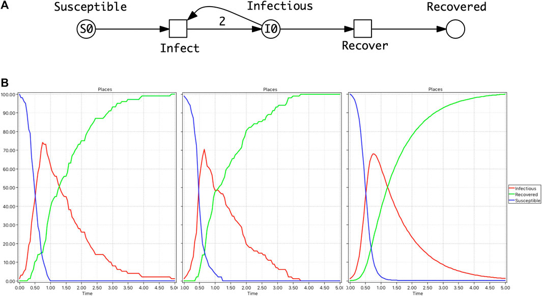
FIGURE 1. SIR model. (A) A Petri Net describing the SIR model where Petri net places (circles) represent the Susceptible (S), Infectious (I) and Recovered (R) compartments. Petri net transitions (squares) represent the actions (events) of becoming infectious and recovering, and arcs connect places with transitions enabling events to occur and describing the effect of the occurrence. At the Infect transition, an infection will only occur when a susceptible and infectious person meet reducing the number in both compartments by 1. This results in two people being added to the Infectious place which is represented by an arc weight of 2 (shorthand notation for two arcs). Note that the default arc weight of 1 is not given. Also the number of infectious people can be reduced by 1 via the Recover transition, increasing Recovered by 1. Each transition preserves the number of persons (the number of incoming arcs equals the number of outgoing arcs), thus the net is conservative and the total population size is constant. (B) From left to right: Two single stochastic runs and the deterministic run, with the initial marking (state): S0 = 100, I0 = 1, and rate constants k_infect = 0.1, k_recover = 1. Note, in the second stochastic run, Infectious dies out much earlier than in the deterministic simulation.

The infection rate is effectively the observed increase in the number of daily infections, more generally the number of infections in a given time period, typically described by mass action kinetics (Wilson and Worcester, 1945). An alternative approach, called the standard incidence, normalises the infection rate by the total population size N, based on the assumption that daily encounters between individuals in the population are largely independent of community size (Hethcote, 2000). The rate constant of infection k_infect (the parameter for mass action kinetics) is driven by both the infectiousness of the disease, as well as any societal prevention measure in place (isolation, etc.). Likewise, the recovery rate is governed by the rate constant of recovery k_recover which reflects the contribution of all the factors contributing to recovery—health of the individuals in the population, treatment etc.

These infection and recovery rates correspond to the rate functions associated with the transitions Infect and Recover in the Petri net model. Rate functions can be interpreted in two different ways: stochastic or deterministic, thus yielding stochastic Petri nets ($\mathcal{SPN}$) or continuous Petri nets ($\mathcal{CPN}$). The semantics of $\mathcal{SPN}$ is given by continuous time Markov chains (CTMC), and the semantics of $\mathcal{CPN}$ by Ordinary Differential Equations (ODEs). The ODEs generated reading the Petri net in Figure 1 as a $\mathcal{CPN}$ are given in Eq. 1, which correspond exactly to the ODEs given in the literature. We observe that each place gets its own equation (see Section 3 for the automatic translation of $\mathcal{CPN}$ into ODEs). In the equations we have replaced the long place names by their standard short forms for readability. The formulae governing the rates according to the standard incidence can be easily adjusted to use the mass action kinetics by setting N = 1.

$\frac{dS}{dt}=-k_{infect}\cdot \frac{S}{N}\cdot I(1)$

$\frac{dI}{dt}=k_{infect}\cdot \frac{S}{N}\cdot I-k_{recover}\cdot I$

$\frac{dR}{dt}=k_{recover}\cdot I$

To obtain a flexible model, we introduce constants S₀, I₀ and R₀ to initialise the places Susceptible, Infectious and Recovered; thus, N = S₀ + I₀ + R₀. In general, the initial values of all the places in a model form its initial state at time t = 0. We also use, for example, the notation S₀ to stand for the value of S_t=0, or generally S_t for time point t.

These models are typically simulated, which for $\mathcal{SPN}$ means making random walks through the CTMC, applying, e.g., Gillespie’s stochastic simulation algorithm (SSA) (Gillespie, 1976), and for $\mathcal{CPN}$ solving the underlying ODEs. Figure 1B gives simulation traces for both cases. Even without realistic rate constants, this basic model already permits some interesting computational experiments, see Section 2.7.

We make some observations about the behaviour of the system. There is a trivial, i.e., disease free steady state for I₀ = 0 so that no infections or recovery occur, otherwise the steady state is reached when I_t = 0. We note some interesting $\mathcal{SPN}$ behaviour of single runs—there is a probability that the infection dies out early, whatever the balance between the rates of infection and recovery, due to the underlying Markov chain. In contrast, the ODE behaviour can be thought of as the average over many stochastic runs, and thus ignores the variability inherent in a stochastic model. Besides exploring time series of model variables, we can also define derived measures as observers, such as the reproduction number $\mathcal{R}$ (Heffernan et al., 2005; van den Driessche, 2017); see Section 3 for details.

All our models can be equally read as $\mathcal{SPN}$ or $\mathcal{CPN}$, or as a Hybrid Petri net ($\mathcal{HPN}$), which is a combination of these two.

2.2 Extended Epidemic Models

The SIR model can be extended by extra compartments such as deaths (D), maternally-derived immunity (M), exposed/incubation period (E), etc., and extra variables such as total number of infectious, total deaths, mutant, etc., yielding variations of the basic SIR model including SIS, SIRS, SIRD, MSIR, SEIR, SEIS, MSEIR, MSEIRS (Hethcote, 2000). Their representation as a Petri net model is straightforward, and Petri net animation supports the modeller in getting the model structure right.

Here we consider four examples which are relevant to the current COVID19 epidemic:

• SIVR—an SIR model extended by a virus variant, represented as an $\mathcal{HPN}$, in this case together with its hybrid simulation trace (Figure 2).

• SIQR model which describes, as an additional route to recovery, the possibility of infectious people being subject to quarantine before recovery (Anand et al., 2020) (Figure 3A).

• SIAR model which differentiates infectious people into symptomatic and asymptomatic compartments (Sen et al., 2017) (Figure 3B).

• SIXR model describing a vaccination regime which assumes that the vaccine needs to be delivered to a person in two doses, and that the person will be vulnerable to some extent between the first and second dose (Figure 4).

FIGURE 2

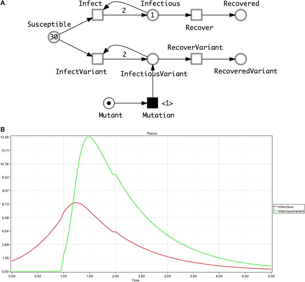
FIGURE 2. SIVR model. (A) $\mathcal{HPN}$ describing the introduction of a virus variant, using a deterministic transition Mutation which fires with a delay of 1 time unit after simulation start, while all other nodes are continuous (indicated by thick grey pen). Kinetic parameters: ratio between Infect and Recover, RecoverVariant is 1:10; ratio between Infect and InfectVariant is 1:5. (B) Hybrid simulation trace for Infectious and InfectiousVariant.

FIGURE 3

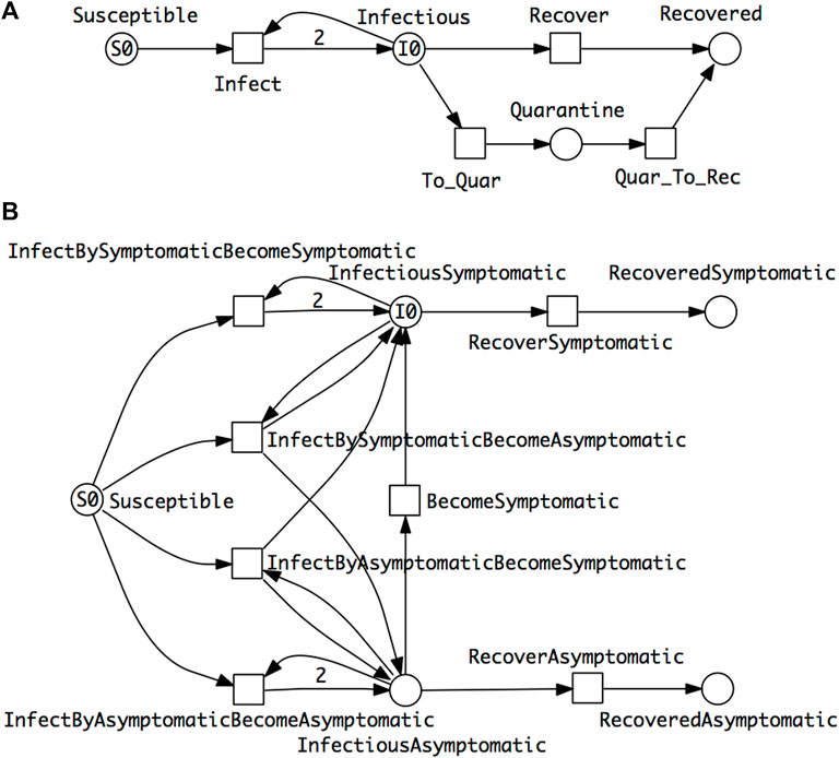
FIGURE 3. Two extended epidemic models. (A) SIQR—an SIR model extended by quarantine. (B) SIAR—an SIR model with symptomatic/asymptomatic compartments. There are four different cases of infection reflected by the four transitions connected with the Susceptible place. The two which involve only one infectious compartment—InfectiousSymptomatic or InfectiousAsymptomatic—follow the standard SIR pattern, reflected in the outgoing arc weights of 2. In the cases of the two dual outcome infections—Susceptible and InfectiousSymtomatic to InfectiousAsymptomatic or vice versa, there are two outgoing arcs to the two infectious places each of which has an arc weight of 1 (not shown by default). The total rate of infection in the whole population is the sum of the rates of the four infection transitions. The ODEs of these two models are given in the Supplementary Material.

FIGURE 4

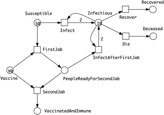
FIGURE 4. SIXR model describing a vaccination regime which assumes that the vaccine needs to be delivered to a person in two doses, and that a person will be vulnerable to some extent between the first and second dose. The amount of vaccine available (V0) may be less than that required to doubly vaccinate the entire susceptible population (S0). However, some people may become immune through infection or die before they are partially or fully vaccinated.

All these Petri nets can be animated in a purely qualitative manner at https://www-dssz.informatik.tu-cottbus.de/DSSZ/Research/ModellingEpidemics.

2.3 Stratified Epidemic Models

In general, modelling the stratification of a population in terms of epidemics means that the overall population is partitioned into a number of strata and a suitable model is defined for each stratum and their appropriate interconnections. The compartments are equally divided into disjunctive sets, such that each partition is internally homogeneous and distinctively differs from all the other partitions, and there are corresponding partitions in all compartments.

In the following we assume that the same epidemic model is equally applied to each stratum. As an example we consider SIR-${\mathrm{S}}_2^{\text{age}}$, an SIR model with two age strata (Figure 5A); see Section 2.6 for an explanation of our naming convention for models.

FIGURE 5

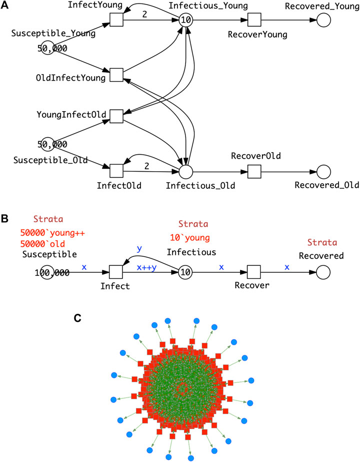
FIGURE 5. SIR-${\mathrm{S}}_{2\text{;}20}^{\text{age}}$ models. Two variations of the SIR model describing stratification of a population into two age groups (young and old) or 20 age groups, and the cross infections between the groups. Transmission of infection does not change the age group of the infectious person. At the start there are no old infectious people, and only very few young infectious people. (A) $\mathcal{CPN}$ for two age strata, each of which is associated with a separate, but structurally identical SIR model, and linked by cross infections. (B) The same model represented as a coloured $\mathcal{CPN}$. The markings of coloured places always show the sum of the markings of the corresponding uncoloured places. The colour definitions are given in Section 3, and the ODEs in the Supplementary Material. (C) Unfolded $\mathcal{CPN}$ of a 20-strata SIR model, with coloured graphics.

Clearly the stratification in this model is very minimal; the standard practice when collecting statistics of infections is to use more than two age groups—often in 10 deciles from 0 to 100 years old. A model should describe all the possible combinations of cross infections, in this case we obtain 10⋅10 = 100 infect transitions. The modelling effort invites modelling errors; this will be further compounded if gender is added to age in the stratification. To cope with this modelling challenge, we use coloured Petri nets, which provide an elegant solution to the given combinatorial problem by pattern compression of the repeated parts (components) of a Petri net, while maintaining the overall structure. Each repeated component is associated with a unique integer (“colour”); see Section 3 for details. This colouring principle, supporting component-based model construction, can be equally applied to $\mathcal{SPN}$, $\mathcal{CPN}$ or $\mathcal{HPN}$, yielding coloured $\mathcal{SPN}$ ($\mathcal{SPN}$^C), coloured $\mathcal{CPN}$ ($\mathcal{CPN}$^C) or coloured $\mathcal{HPN}$ ($\mathcal{HPN}$^C).

In summary, Figure 5 gives the same model in two different but equivalent representations, uncoloured (Top) and coloured (Middle), which also means that both generate the same ODEs. Obtaining the coloured model from the uncoloured one is called folding (compression), and the reverse operation is called unfolding (expansion). Folding is typically performed manually because the degree of folding is subjective, while unfolding can be done automatically as long as all colour sets are discrete and finite.

Increasing the number of strata while ensuring that all needed connectivities are present just requires extending the colour set Strata; nothing else in the structure of the coloured model needs to be touched, apart from adjusting the initial marking. In this way, our modelling approach supports scalability in an easy to use manner. In general the unfolded SIR model for s strata comprises 3s places, s² + s transitions and 4s² + 2s arcs, and the ODEs generated consist of 3s equations.

2.4 Pandemic Models

The distinguishing characteristic of a pandemic model is the concept of multiple intercommunicating epidemic models in a spatial (geographic) context. In the following we prefix standard epidemic model names by ‘P’ for pandemic, thus obtaining PSIR, PSIVR, PSIQR, etc.

2.4.1 Two Countries, Linked by Travel

Figure 6A shows a PSIR model comprising epidemic SIR models in each of two countries, with population movement permitted between the countries for all compartments. As for the age strata model, we can fold it into a coloured version (Figure 6B). The process of colouring is very similar to that described for SIR-${\mathrm{S}}_2^{\text{age}}$ (see Section 3).

FIGURE 6

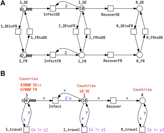
FIGURE 6. P₂SIR model. (A) $\mathcal{CPN}$ for two countries, each of which is associated with a separate, but structurally identical SIR model, and linked by travel. (B) The same model represented as a coloured $\mathcal{CPN}$. Eeach travel transition is associated with a guard [x != y] (x and y are unequal) to ensure that travellers do not immediately return to their country of origin. The uncoloured and coloured model are equivalent, thus generate the same ODEs, which are given in the Supplementary Material.

2.4.2 N Countries, Linked by Travel

Generalising this idea to more than two countries, the travel connectivities between countries need to be defined. For example, when considering surface travel, not all countries are directly connected to each other. We assume that the connectivity is described by a graph (Figure 7A); this could be directly encoded as a standard Petri net (Figure 7B), which we fold for convenience into a coloured Petri net (Figure 7C), see Section 3 for details. Equally the graph could include air and/or sea connections; even then, connectivity could still be less than fully connected.

FIGURE 7

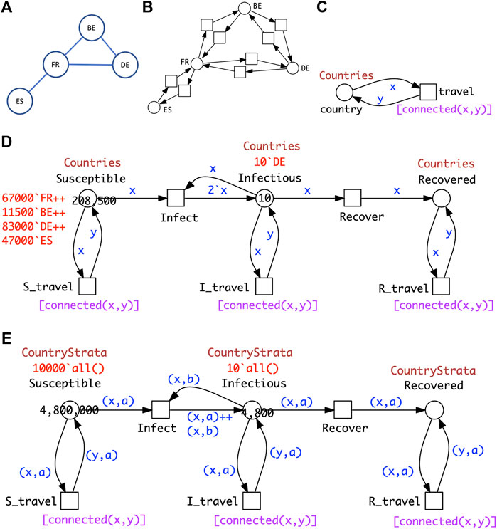
FIGURE 7. P_nSIR models. (A) Connectivity graph for four countries. (B) Petri net representation of the connectivity graph. (C) Coloured Petri net representation of the connectivity graph; see Section 3 for details. (D) Coloured Petri net representation of the pandemic P₄SIR; structural identical with P₂SIR in Figure 6B; both ${\mathcal{CPN}}^{\mathcal{C}}$ differ by their colour definitions encoding different connectivity graphs. The unfolded Petri net of P₄SIR is give in Supplementary Figure S2. (E) P₄₈SIR-${\mathrm{S}}_{10}^{\text{age}}$ coloured Petri net for 48 countries in Europe, each with 10 age strata, see Figure 9 for its unfolded version.

The coloured Petri net representation of the PSIR over four countries (Figure 7D) is derived by adjusting the colour definitions in the SIR for two countries (Figure 7E) according to the connectivity graph, and getting the initial marking right.

The generalisation to connectivity graphs representing different geographical relationships is straightforward, merely requiring adjusting the two related colour definitions (Countries, Connections) and the initial marking. This example illustrates how our modelling approach supports reusability in an easy to use manner. In general the unfolded PSIR model for n countries with overall m mutual connections comprises 3n places, 2n + 6m transitions and 6n + 12m arcs, and the ODEs generated consist of 3n equations.

We provide a number of PSIR pandemic models in the Supplementary Material, including Europe (P₁₀SIR: 10 countries, 15 mutual connections, P₄₈SIR: 48 countries, 85 mutual connections), China (P_ChinaSIR: 34 provinces, 71 mutual connections) and the United States (P_USASIR: 50 states, 105 connections), and the guidelines how to obtain the corresponding ODEs using our tool platform. For illustration, we give the connectivity graph and deterministic simulation traces for P₁₀SIR in Figure 8.

FIGURE 8

FIGURE 8. P₁₀SIR behaviour. (A) Connectivity graph for 10 Western European countries connected by road. AT = Austria, BE = Belgium, CH = Switzerland, DE = Germany, DK = Denmark, ES = Spain, FR = France, IT = Italy, NL = Netherlands and PT = Portugal. (B) Traces of modelled infections. Plots for countries under 100 Infectious are not visible due to the scale of the graph.

2.5 Combined Models

These three extensions—SIR variations, stratification and space—are orthogonal, and thus any combination is possible. For illustration we provide two examples:

• P₁₀SIQR combining space (Europe with 10 countries) with an extended epidemic model (Supplementary Figure S3) which yields 4n = 40 ODEs, and

• ${\mathrm{P}}_{48}{\mathrm{S}\mathrm{I}\mathrm{R}-\mathrm{S}}_{10}^{\text{age}}$ combining space (Europe with 48 countries) and stratification (10 age strata per country; coloured version in Figure 7E, unfolded version in Figure 9) which yields 1,440 ODEs.

FIGURE 9

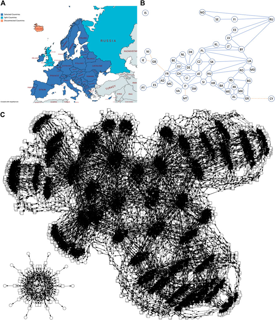
FIGURE 9. P₄₈SIR-${\mathrm{S}}_{10}^{\text{age}}$ model (A) Map of 48 European countries created with https://mapchart.net. (B) Undirected graph representation of the map where edges represent two-way surface connections. Blue edges stand for road connections, orange dashed edges for sea connections. (C) Unfolded version of the coloured net in Figure 7E; unfolding takes about 1 s on a standard laptop computer; layout automatically generated. Iceland appears as an isolated subnet because it is not connected by surface to the rest of Europe, and is thus similar to the SIR net with 20 strata in Figure 5C. Model size: 1,440 places; 10,380 transitions. With initially 100,000 susceptible persons per strata in every country, making a total population of 48,000,000, continuous simulation up to simulation time 1 takes less than 1 min and stochastic simulation (Gillespie’s SSA, single run) about 4 min.

In general the unfolding of a P_nSIR-S_s model with s strata and n countries with m mutual connections comprises 3sn places, n(s² + s) + 6 ms transitions and 2n(2s² + s) + 12 ms arcs.

2.6 Model Summary

Table 1 provides a summary of the models provided. The naming convention of our models basically follows the Extended BNF given in Table 2.

TABLE 1

TABLE 1. Summary table of models. I Basic and extended epidemic models. II Stratified models. III Pandemic models. IV Combined models; CANDL files provided as separate files in Supplementary Material.

TABLE 2

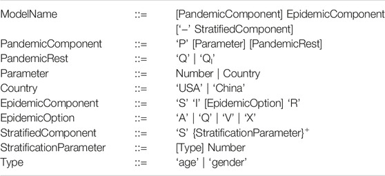
TABLE 2. Extended BNF for model naming convention.

2.7 Parameter Fitting

Apart from defining the structure of a model, it is also important to find suitable rate constants. This can be naively achieved by scanning over parameter values, or in a more sophisticated manner heuristically by target driven parameter optimisation.

Even without fitted values derived from real world data, a great deal of useful analysis can be achieved using comparative rate constant values. Examples include scanning by

• Varying the ratio between infection rate and recovery rate while maintaining the recovery rate constant resulting in changes in the ${\mathcal{R}}_t$ value (SIR), and comparison between geographic regions (PSIR),

• Varying the ratio between direct and quarantine recovery (SIQR), and varying quarantine regimes (see Supplementary Figures S5, S6 both referring to the model P₁₀SIQR in Supplementary Figure S3 (Top)).

• Varying the initial state of the infectious compartments in the different countries of a pandemic model (PSIR),

• Varying the strength of the connectivities between countries—road, train, sea and air—in a pandemic model (PSIR).

Refining a model automatically involves increasing the number of required kinetic rate constants. Specifically in the SIR-${\mathrm{S}}_2^{\text{age}}$ model, the kinetic constants can be different for both intra-stratum and inter-strata transitions. This can be achieved in the coloured version using colour-dependent rates, see Section 3.

More generally, we can establish equivalence classes for rate constants, for example in a PSIR travel model, there can be different rate constants between classes of movements such as road versus air and/or frequent versus rare, while the rate constants within classes are the same.

When real world data are available, then we can attempt to fit models to them. We did this for the pandemic model for ten European countries (P₁₀SIR, Supplementary Figure S6), based on source data for daily new infections obtained from WorldOmeters (https://www.worldometers.info/coronavirus/) during the period 19th January to 16th August 2020. The rate constants fitted were for infection, and the inter-country movement for all three compartments. The values for the Susceptible, Infectious and Recovered compartments for movement in one direction between a pair of countries were kept the same, thus reflecting the assumption that the rate constant for travel does not depend on the compartment, but only on the journey. Initial markings for Infectious were set at 1% of the total population for each country according to Wikipedia, divided by 1,000. Daily new cases were standardised and smoothed using a 7-day rolling average (Supplementary Figure S7) and the magnitude and timing of the peaks were detected computationally (Supplementary Table S1).

The goals of the fitting were (Objective 1) to reproduce the order of the time taken from the first five deaths to a peak for daily new cases, (Objective 2) to reproduce the order of the height of the peaks for daily new cases, and (Objective 3) combining Objective 1 and Objective 2. Fitting was performed in all three cases using target driven optimisation employing Random Restart Hill Climbing (see Section 3 for details, and Supplementary Tables S2–S5).

2.8 Analysis

For an initial validation of (unfitted) pandemic model behaviour we performed correlation analyses between real world variables and model variables for P₁₀SIR and P₄₈SIR; for details see Supplementary Table S6 and Supplementary Figures S8, S10. These results support our assumption that even the unfitted pandemic models behave well, and that the geography incorporated into the model appropriately influences behaviour. Thus, an analysis of the unfitted pandemic PSIR model can give useful insights even in the absence of detailed real data; specifically given the geographical connections between regions and their populations, we can predict to some extend the expected peak height of infections and thus inform planners how to cope with the impact on health services, etc, ; some examples are given below.

An initial analysis can be performed by inspection of the visualised time series plots. Properties of interest include the values of Susceptible and Recovered over time (e.g., for herd immunity), and the existence, order and height of peaks for Infectious, see, e.g., Figure 8. This can be extended to derived measures such as the $\mathcal{R}$ value, computed over time and plotted for the different geographic regions.

Going beyond visual inspection, the order and height of peaks can be ascertained computationally from the traces. More generally, many behavioural properties of interest can be expressed using linear temporal logic and analysed in practice via simulative model checking (Donaldson and Gilbert, 2008; Gilbert et al., 2019), which is specifically useful for exploring larger models by the use of property libraries, see Section 3 and Figure 10.

FIGURE 10

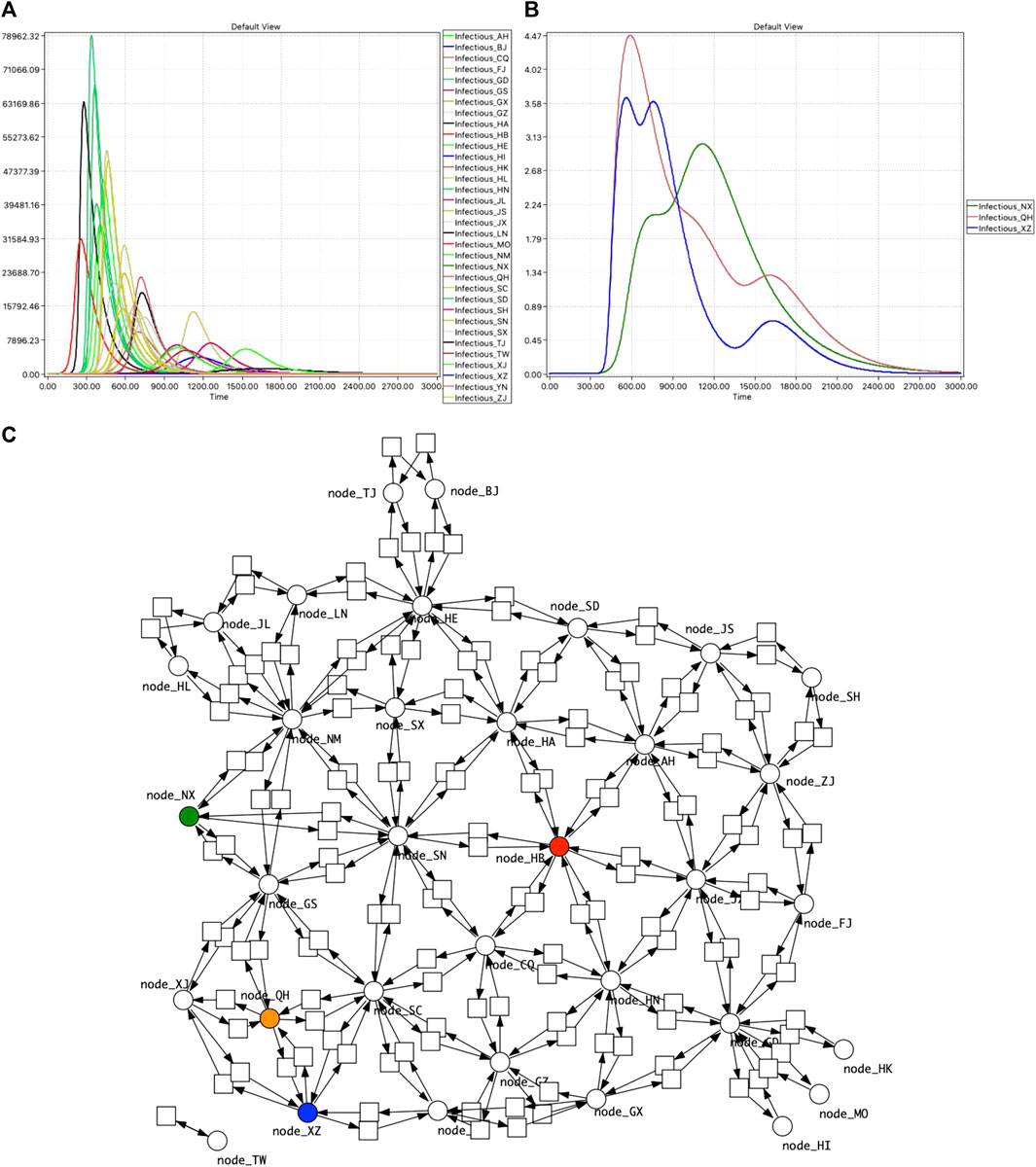
FIGURE 10. P_ChinaSIR model checking. (A) Time series traces of Infectious for the 34 provinces, with infection starting in Hubei. The ratio between rate constants for Infect and Recover is 1:10⁴ (k_infect = 1.0e⁻⁶, k_recover = 1.0e⁻²). (B) Model checking reveals three provinces with more than one peak. (C) Network of China highlighted to indicate the geographical context of the three provinces: HB—red, NX—green, QH—brown, XZ—blue.

In addition, the general relationships between the behaviour of related compartments or derived measures in different geographical regions can be determined via cluster analysis. The results for hierarchical clustering can be represented, for example, via dendrograms, see Supplementary Figures S11, S12.

Furthermore, the results of such comparative analyses above could be related to the genomic data of the causative infectious agent, for example, a virus which exhibits high mutation rates. Thus the variants or strains of the virus which evolve over the time of an epidemic can be related to the behaviour of pandemic models.

Finally, pandemic models can be used to predict the effects of various control measures. These include travel restrictions in terms of inter-country connections, and quarantine restrictions on international travellers. In addition, the effects of the imposition and lifting of lockdowns in different regions and at different times can be investigated, but requires the dynamic variation of rate constants during simulation. In order to facilitate this, we have recently extended the Spike simulator to include event-driven triggers, which enables the modelling of these control measures, for an example see Figure 12.

Given a pandemic PSIR model with fitted parameters, as developed in the previous section, we can perform a detailed comparative analysis over the geographic regions, going beyond the analysis based on comparative values.

3 Methods

3.1 Related Work

In order to put our work in context, we give a brief overview of related work. A general review paper on epidemic modelling including metapopulation models can be found in (Brauer, 2017). Early basic pandemic approaches include mathematical models based on ODEs for the global spread diseases, where travel connectivity is described by adjacency matrices (Rvachev and Longini, 1985; Longini, 1988), and by graphs (Sattenspiel and Powell, 1993; Sattenspiel and Dietz, 1995). However, the ODE formalism does not incorporate features which support component-based model design and construction; thus there is no natural way to move from simple SIR-like epidemic models to pandemic models comprising SIR components in a spatio-temporal relationship.

Some recent case studies incorporating spatial aspects include (Chen et al., 2014) considering dynamics of a two-city SIR epidemic model and (Aràndiga et al., 2020; Goel and Sharma, 2020) for the current COVID-19 pandemic. However none of the models are downloadable and adaptable.

The GLEaM, viz, computational tool (Van den Broeck et al., 2011) has been developed to model multiscale mobility networks and the spatial spreading of infectious diseases building on a series of papers including (Colizza and Vespignani, 2008; Balcan et al., 2009; Balcan et al., 2010) and has been used to model the 2009 H1N1 pandemic (Bajardi et al., 2011). Although the core epidemic model components can be exported, the spatio-temporal data (geographical relationships, mobility and population) cannot.

The Spatiotemporal Epidemiologic Modeler (STEM) is an Eclipse based monolithic framework to support the development and simulation of geographic disease models (Edlund et al., 2010). It builds on a component-based architecture (plugins); models can be simulated deterministically or stochastically. Models are encoded in Java, and it is not obvious how to export a model if one wants to apply any analysis technique not supported by the framework.

Age-based stratification has been addressed in, for example, (Del Valle et al., 2013; Balabdaoui and Mohr, 2020), and the effects of intervention strategies for COVID19 in Balabdaoui and Mohr (2020), Giordano et al. (2020), Prem et al. (2020).

Other approaches besides ODE modelling include stochastic models (Nandi and Allen, 2019)—not spatio-temporal, and (Oka et al., 2020)—a case study on China, agent-based models (Mahmood et al., 2020) and coloured Petri nets (Castagno et al., 2020)—the latter being without spatio-temporal aspects.

Some groups have developed methods for simulating Petri nets directly at the coloured level (Beccuti et al., 2015; Cardelli et al., 2017). However these techniques are only applicable to symmetric nets; none of the coloured models reported in this paper conform to this constraint.

In the following we describe the methods underlying our technology.

3.2 Modelling

3.2.1 Modelling Assumptions

Our approach employs compartment-based modelling principles, where the population is divided into a set of homogeneous compartments. For example, the population in the basic SIR model population is divided into three compartments—Susceptible (S), Infectious (I) and Recovered (R). These three compartments are considered to be homogeneous, thus there is an equal probability of any event occurring to any member of each compartment.

We also assume for all our models that a susceptible person is infected by an infectious person so that they are both infectious; thus getting infected and becoming infectious coincide. A susceptible person can become recovered. In the traditional SIR model, recovered people are resistant and cannot become susceptible or infectious. Although this model was widely used to describe the behaviour of the COVID-19 epidemic, it became clear that the assumption regarding the resistance of recovered people to reinfection did not hold as new variants of the virus emerged. Thus an SEIS (Susceptible, Exposed, Infectious, Susceptible) model was more relevant for that situation.

Our models do not consider births or natural deaths so that the total population size is constant, as can be seen, e.g., from the structure of the SIR model in Figure 1, which shows a conservative Petri net covered by a single minimal P-invariant (compare paragraph below on Petri net analysis techniques). However, the models could be easily extended to incorporate births and/or deaths, without any impact on their ability to be simulated.

It is also generally assumed that S₀ ≫ I₀, and (for obvious reasons) I₀ > 0 and R₀ = 0.

3.2.2 Petri Nets

Petri nets are a family of formal languages which come with a graphical representation as bipartite directed multi-graphs, enjoying an operational (execution) semantics. They can be either untimed and qualitative, or timed and quantitive; for details see (Heiner et al., 2008). All these net classes share the following graph properties.

• Bipartite: There are two types of nodes, called places and transitions, which form disjunctive node sets. Places, graphically represented as circles, typically model passive objects (here compartments and derived measures, possibly in different locations), while transitions, graphically represented as squares, model active events (such as infect, recover, travel), changing the state of the passive nodes.

• Directed: Directed arcs, represented as arrows, connect places with transitions and vice versa, thereby specifying the relationship between the passive and active nodes. The bipartite property precludes arcs between nodes of the same type.

• Multigraph: Two given nodes may be connected by multiple arcs, typically abbreviated to one weighted arc. The weight is shown as a natural number next to the arc. The default value is 1, and usually not explicitly given.

The execution semantics builds on movable objects, represented as tokens residing on places. The number zero is the default value, and usually not explicitly given. The current state (marking m) of a model is defined by the token situation on all places, usually given by a place vector, which is a vector with as many entries as we have places, and the entries are indexed by the places. The initial state is denoted by m₀.

The specific details of the execution semantics slightly differ for qualitative and quantitative Petri nets, and if the Petri net class belongs to the discrete or continuous modelling paradigm.

We start off with standard Petri nets, which are inherently untimed and discrete. Their (non-negative integer) token numbers are given by black dots or natural numbers. The current state is given by the number of tokens on all places, forming a place vector of natural numbers. The (integer) arc weights specify how many of these tokens on a certain place are consumed or produced by a transition, causing the movement of tokens through the net, which happens according to the following rules (Blätke et al., 2015):

• Enabledness: A transition is enabled, if its pre-places host sufficient amounts of tokens according to the weights of the transition’s ingoing arcs. An enabled transition may fire (occur), but is not forced to do so.

• Firing: Upon firing, a transition consumes tokens from its pre-places according to the arc weight of the ingoing arcs, and produces new tokens on its post-places according to the arc weights of the outgoing arcs. The firing happens atomically (i.e., there are no states in between) and does note consume any time. Firing generally changes the current distribution of tokens; thus the system reaches a new state.

• Behaviour: We obtain the dynamic behaviour of a Petri net by repeating these steps of looking for enabled transitions and randomly choosing one single transition among the enabled ones to let it fire.

3.2.3 Rate Functions

These standard untimed Petri nets, which are entirely qualitative, can be extended by enriching transitions with firing rate functions. We obtain timed and thus quantitive Petri nets, out of which we use in this paper stochastic Petri nets ($\mathcal{SPN}$) generating continuous time Markov chains, and continuous Petri nets ($\mathcal{CPN}$) generating Ordinary Differential Equations (ODEs). Both net classes merely differ by the interpretation of the rate functions; thus $\mathcal{SPN}$ and $\mathcal{CPN}$, sharing the same net structure, can be easily converted into each other.

Rate functions are, technically speaking, arbitrary mathematical functions, typically depend on the given state, and are often governed by popular kinetics, such as mass action kinetics (Wilson and Worcester, 1945).

Stochastic rate functions specify how often a transition occurs per time unit, technically achieved by stochastic waiting times before an enabled transition actually fires. $\mathcal{SPN}$ with exponentially distributed waiting times for all transitions fulfil the Markov property; thus their semantics are described by continuous time Markov chains (CTMC), and the current state of an $\mathcal{SPN} \mathrm{is\; still\; defined\; by\; a\; place\; vector\; of\; natural}\mathrm{numbers.\; The\; CTMC\; for\; a\; given} \mathcal{SPN}$ is basically isomorphic to the state transition system of its corresponding untimed Petri net. Thus, all Petri net analysis techniques (see Section 3.2.7) can still be applied, and all behavioural properties that hold for the untimed Petri net are still valid for the corresponding $\mathcal{SPN}$.

In contrast, deterministic rate functions define the strength of a continuous flow, turning the traditionally discrete modelling paradigm of Petri nets into a continuous one: the discrete number of tokens on each place is replaced by a (non-negative) real number, called token value. Thus, the current state of a $\mathcal{CPN}$ is defined by a place vector of real numbers. A $\mathcal{CPN}$ transition is enabled if the token value of all its pre-places is larger than zero. This coincides for mass action kinetics with transition rates larger than zero. Due to the influence of time, a continuous transition is forced to fire as soon as possible. Altogether, the semantics of a $\mathcal{CPN}$ is defined by ODEs.

3.2.4 How to Transform a $\mathcal{CPN}$ into Ordinary Differential Equations

Each place subject to changes gets its own equation, describing the continuous change over time of its token value by the continuous increase of its pre-transitions’ flow and the continuous decrease by its post-transitions’ flow. Thus, in the generated ODEs, places are interpreted as (nonnegative) real variables. A transition that is pre- and post-transition for a given place yields two terms, which can be reduced by algebraically transforming the right-hand side of the equation. Thus, each equation corresponds basically to a line in the incidence matrix (Heiner et al., 2008).

To formalise the transformation of $\mathcal{CPN}$ into ODEs, we need to introduce a few technical notations. Let ^•p denote the set of pre-transitions of the place p, and p^• the set of post-transitions, $v\left(t\right)$ gives the rate function for transition t, $f\left(t,p\right)$ the weight of the arc going from t to p, and $f\left(p,t\right)$ the weight of the arc going from p to t. Then the ODE generated for the place p is given by Eq. 2.

$\frac{d\left(p\right)}{dt}=\sum _{t{\in }^{•}p}f\left(t,p\right)v\left(t\right)-\sum _{t\in p^{•}}f\left(p,t\right)v\left(t\right)(2)$

In words: the pre-transitions t ∈ ^•p increase the token value of p, thus their weighted rate functions occur as plus terms, while the post-transitions t ∈ p^• decrease the token value of p, thus their weighted rate functions occur as minus terms of the ODE’s right hand side.

The models presented in this paper always generate as many ODEs of this style as we have places. This is automatically triggered when simulating a $\mathcal{CPN}$, which can be done in our platform either with Snoopy or Spike. In summary, $\mathcal{CPN}$ can be seen as a structured approach to write ODEs (Breitling et al., 2008); they uniquely define ODEs, but generally not vice versa, compare (Soliman and Heiner, 2010; Heiner and Gilbert, 2011).

3.2.5 Coloured Petri Nets

Coloured Petri nets combine Petri nets with the powerful concept of data types as known from programming languages (Genrich and Lautenbach, 1981; Jensen and Kristensen, 2009). Tokens are distinguished via colours; there are no limits for their interpretation. For example, colour allows for the discrimination of compartments by, e.g., age strata or gender, or to distinguish compartments in different geographical locations. In short, colours permit us to describe similar network structures in a compressed, but still readable way. A group of similar model components (subnets) is represented by one component coloured with an appropriate colour set, and the individual components become distinguishable by a specific colour in this colour set. See (Liu et al., 2019) for a review of the widespread use of coloured Petri nets for multilevel, multiscale, and multidimensional modelling of biological systems.

Coloured Petri nets consist, as uncoloured Petri nets, of places, transitions, and arcs. Additionally, a coloured Petri net is characterised by a set of discrete data types, called colour sets, and related net inscriptions.

• Places get assigned a colour set and may contain a multiset of distinguishable tokens coloured with colours of this colour set. Our PetriNuts platform supports a rich choice of data types for colour set definitions, including simple types (dot, integer, string, Boolean, enumeration) and product types.

• Transitions get assigned a guard, which is a Boolean expression over variables, constants and colour functions. The guard must be evaluated to true for the enabling of the transition. The trivial guard true is usually not explicitly given.

• Arcs get assigned an expression; the result type of this expression is a multiset over the colour set of the connected place.

• Rate functions may incorporate predicates, which are again Boolean expressions. They permit us to assign different rate functions for different colours (colour-dependent rates). Otherwise, the trivial predicate true is used; for examples see Supplementary Material.

Elaborating the behaviour of a coloured Petri net involves the following notions (Blätke et al., 2015).

• Transition instance: The variables associated with a transition consist of the variables in the guard of the transition and in the expressions of adjacent arcs. For the evaluations of guards and expressions, values of the associated colour sets have to be assigned to all transition variables, which is called binding. A specific binding of the transition variables corresponds to a transition instance. Transition instances may have individual rate functions.

• Enabling: Enabling and firing of a transition instance are based on the evaluation of its guard and arc expressions. If the guard is evaluated to true and the pre-places have sufficient and appropriately coloured tokens, the transition instance is enabled and may fire. In the case of quantitative nets, the rate function belonging to the transition instance is determined by evaluating the predicates in the rate function definition.

• Firing: When a transition instance fires, it consumes coloured tokens from its pre-places and produces coloured tokens on its post-places, both according to the arc expressions. which generally results into a new state.

3.2.5.1 Colouring Example

Let us illustrate the use of colour by means of the stratified age SIR example (SIR-${\mathrm{S}}_2^{\text{age}}$), see Figure 5. The common pattern is a single basic SIR model. In order to design the coloured model, shown in Figure 5C, we introduce an enumerated colour set Strata = {young, old} (where each element is internally mapped onto an integer) and two variables of this colour set x and y, each of which can hold either young or old. Arcs in this model are now labelled with expressions over these variables. The bindings to the variables are considered only in the local environment (incoming and outgoing arcs) of each transition. The incoming and outgoing arcs of the coloured transition Recover are both labelled with the same variable x because that transition only operates within one stratum. However the coloured transition Infect has connections both within one stratum and between strata; this is accomplished by using the two variables x and y on the two incoming arcs from Susceptible and Infectious, each of which independently hold as bindings either young or old, giving in total four combinations, two of which standing for the inter-strata cross infections and the other two for the intra-stratum infections. The x represents the person who becomes infectious, and y the infecting person. Thus the outgoing arc from the transition to the place Infectious is labelled with the multiset {x,y} written as x ++ y. If x and y hold the same colour, x ++ y corresponds to an arc weight of two in the standard Petri net model.

3.2.5.2 Folding/Unfolding

Any (standard) Petri net can be folded into a coloured Petri net comprising just a single (coloured) place and a single (coloured) transition. Then, the entire structure is hidden in the colour definitions, which can always be revealed by automatic unfolding. Generally, the decision regarding how much structure to fold into colours is a matter of taste. We follow the rule that a model should be still completely comprehensible by reading the structure and its colour annotations. In general, folding of epidemic models should preserve the pattern of the SIR (or related) model. For illustration, we provide a coloured version of the SIAR symptomatic/asymptomatic model in the Supplementary Material.

In principle, coloured Petri nets could be simulated directly on the coloured level with the constraint that the model is symmetric (Beccuti et al., 2015), thus avoiding blowing up the model structure which often comes with unfolding. However, the corresponding algorithms are much more complicated, often involve an implicit partial unfolding, and only a few of them are actually available in practice (Beccuti et al., 2019; Amparore et al., 2021). In addition, our models are generally not symmetric.

In contrast, unfolding to the corresponding uncoloured Petri net can be efficiently achieved (Schwarick et al., 2020) and permits to re-use the rich choice of analysis and simulation techniques, which have been developed over the years for uncoloured Petri nets, including $\mathcal{SPN}$ and $\mathcal{CPN}$, many of them are now supported by highly efficient libraries and reliable software tools.

This is why we exclusively adopt the second approach. All our coloured models are automatically unfolded when it comes to analysing and/or simulating them. In contrast, animation is achieved by unfolding in every step only the transition to fire next; no complete unfolding needs to be generated.

3.2.5.3 Encoding Space and Locality

The use of colour enables us to encode matrices, where colours (natural numbers) represent indices; multidimensional matrices can be represented by appropriate colour tuples. Previously we have used this approach to encode one, two and three dimensional Cartesian space where coordinates were represented as tuples over the entire matrix (Gilbert et al., 2013), for example, modelling diffusion and cell movement in biological systems: planar cell polarity in the Drosophila wing (Gao et al., 2013), phase variation in bacterial colonies (Pârvu et al., 2015), bacterial quorum sensing (Gilbert et al., 2019) and intra-cellular calcium dynamics (Ismail et al., 2020).

In this research we use tuples to index sub-matrices, permitting us to represent graphs as adjacency matrices and hence to encode geographical spatial relationships. This overcomes the limitations of the previous Cartesian coordinate approach for representing pandemics, because whole matrices represent travel diffusion-wise in a regular grid, rather than specific travel connections.

For illustration we consider the encoding of the connectivity graph for four European countries, where connectivity reflects border sharing, see Figures 7A–C. In order to achieve this we define a colour set of enumeration type comprising all countries and next a matrix as a product over this colour set.

colorsets:

enum Countries = {BE,DE,ES,FR};

Matrix = PROD (Countries, Countries);

A subset of the matrix is defined by a Boolean expression (given in square brackets) comprising all required connections.

colorsets:

Connections = Matrix[ // subset defined by Boolean expression

(x=ES & (y=FR)) |

(x=FR & (y=ES | y=BE | y=DE)) |

(x=BE & (y=DE | y=FR)) |

(x=DE & (y=FR | y=BE ))];

Finally we define a colour function connected to be used as guard for the Travel transitions, which constrains travel according to the connectivity graph.

colorfunctions:

bool connected (Countries p, Countries q)

{ (p,q) elemOf Connections };

This acts in the same way as the more simple constraint [x ! = y] used in Figure 6. Now, colour-dependent rates may model different disease control policies in different subpopulations or in different locations.

Besides this, we need two variables of the colour set Countries to be used in the arc inscriptions and thus occurring as parameters in the transition guards.

variables:

Countries: x;

Countries: y;

3.2.6 Framework

These colouring principles can be equally applied to qualitative and quantitative Petri nets, yielding, among others, coloured $\mathcal{SPN}$ ($\mathcal{SPN}$^C) and coloured $\mathcal{CPN}$ ($\mathcal{CPN}$^C): Our PetriNuts platform supports the handling of all of them, which includes the reading of a quantitative Petri net as either $\mathcal{SPN}$ or $\mathcal{CPN}$ (supported by Snoopy and Spike) and the automatic unfolding of $\mathcal{SPN}$^C and $\mathcal{CPN}$^C to their uncoloured counterparts (supported by Snoopy, Marcie and Spike). See Supplementary Figure S1 for an overview of the modelling paradigms integrated in the unifying framework of the PetriNuts platform and the relations among the supported net classes (Heiner et al., 2012).

3.2.7 Petri Net Analysis Techniques

Petri net theory comes with a wealth of analysis techniques (Murata, 1989), some of them are particularly useful in the given context due to the specificity of the net structures of our $\mathcal{SPN}$ and $\mathcal{CPN}$ models, which we obtain by design.

• Conservative: A Petri net is called conservative, if the number of tokens is preserved by any transition firing. This is the case if it holds for all transitions that the sum of the weights of incoming arcs equals the sum of the weights of outgoing arcs. In our models, most of the transitions have exactly one incoming and one outgoing arc, with the exception of Infect transitions which have two incoming and two outgoing arcs (the latter combined to one arc with a weight of 2).

• P-invariant: A P-invariant (as it occurs in the models considered here) corresponds to a set of places, holding in total the same amount of tokens in any reachable state. Generally, P-invariants induce token-preserving subnets. A P-invariant is minimal, if (roughly speaking) it does not contain a smaller P-invariant; see (Heiner, 2009) for details. The models discussed in this paper have the remarkable property that the are covered by non-overlapping minimal P-invariants, and each minimal P-invariant comprises the places (compartments) of one stratum.

Extending a model by cumulative counters, such as the total number of infectious over time, destroys the conservative net structure and induces additional overlapping P-invariants; thus the model is still covered with P-invariants (CPI); see Supplementary Figure S3 for an example.

More generally speaking, any epidemic/pandemic model without birth (transition without pre-place) and/or death (transition without post-place) is covered with P-invariants.

We use both criteria for model validation to avoid modelling mistakes. They are independent of the initial marking and can be easily decided by exploring the net structure only. This is done in our PetriNuts platform by the tool Charlie. Both criteria prove independently the boundedness of a model (the number of tokens on each place is limited by a constant), which ensures in turn a finite state space.

The finite state space could possibly open the door to analyse $\mathcal{SPN}$ models by numerical methods to determine popular Markov properties (Schwarick and Heiner, 2009), such as the probability to reach a (transient) state where, e.g., half of the population is effected. However, a closer look on the typical size of the generated CTMC soon questions this endeavour, as numerical methods rely on a real-numbered square matrix in the size of the state space (Heiner et al., 2010). So we basically have to confine ourselves to simulation and analysis techniques working over simulation traces, such as simulative model checking; see Section 2.8.

It is obvious from exploring the model behaviours that they reach a dead state (there is no enabled transition), as soon as the infectious compartment becomes empty, because there is no way to add something to the infectious compartment as soon as it got empty. In Petri net terms this corresponds to a bad siphon (a siphon not containing a trap); all these are further popular notions of Petri net theory, requiring structural analysis only, while permitting conclusions on behavioural properties; see (Heiner et al., 2008) for details.

Often, epidemic/pandemic models are by design irreversible, reflecting the (optimistic) assumption that a once gained immunity is never lost, and a model will reach a dead state at the very latest when the entire population is recovered. Loosening this assumption by adding a transition from either Infectious or Recovered to Susceptible and refilling Infectious in each epidemic model component will introduce cycles to a model which now becomes a chance to be reversible and live (which in turn precludes dead states), if it is covered with T-invariants; see (Heiner, 2009) for details. This obviously requires that the geographical connectivity graph is strongly connected.

3.2.8 Petri Net Simulation

Besides structural analysis for model validation, we apply simulation techniques generating traces of model behaviour. Simulation traces are time series reporting the current variable values at the n + 1 time points t_i of a specified output grid i = 0, … n, typically splitting the simulation time into n equally sized time intervals. We consider here two basic types of traces:

• traces of place markings, i.e., time series of the current marking (state) of the compartments at the specified time points of the simulation run: $s(t_i):P\to \mathbb{N}$, with s(t₀) = m₀, i.e., s (t_i) are (non-negative) integer place vectors over all place markings, indexed by the set of places P; • traces of transition rates, i.e., time series of the number of occurrences which each individual event had in total in the latest time interval, $v(t_i):T\to \mathbb{N}$, with v(t₀) = 0, i.e., v(t_i) are (non-negative) integer transition vectors over all transition rates, indexed by the set of transitions T.

Reading a transition rate vector as Parikh vector immediately leads us to the state equation specifying the relation between both traces: $s(t_i)=s(t_{i-1})+\mathbb{C}\cdot v(t_i),i=1\dots n$,

where $\mathbb{C}$ is the incidence matrix of a Petri net (Heiner et al., 2008). Thus, the place trace can be derived from the transition trace, but generally not vice versa. In the stochastic setting, the transition trace cannot be uniquely deduced from the place trace due to alternative and parallel transitions, which specifically holds for individual traces. Therefore, we directly record the transition traces during simulation.

Often we consider averaged traces, and the deterministic simulation of $\mathcal{CPN}$ and $\mathcal{CPN}$^C is bound to do so, such that the individual values at each time point are non-negative real numbers $({\mathbb{R^}}^{+})$ instead of natural numbers $(\mathbb{N})$:

$s(t_i):P\to {\mathbb{R^}}^{+}$, with s(t₀) = m₀ (traces of place markings),

$v(t_i):T\to {\mathbb{R^}}^{+}$, with v(t₀) = 0 (traces of transition rates)

Simulation traces may include coloured places/transitions, where a coloured node always gives the sum of the values of the corresponding unfolded nodes. For example, in the SIR-S₂ model given in Figure 5, the coloured place Susceptible always shows the sum of its two unfolded nodes Susceptible_Young and Susceptible_Old; likewise for transitions and their rates.

3.2.9 Derived Measures

A measure often used in the daily news is the daily or weekly number of new infections, given at time point t by

${\mathrm{\Delta }}_t^{I1}=S_t-S_{t-1}or{\mathrm{\Delta }}_t^{I7}=S_t-S_{t-7}.$

These can also be defined by:

${\mathrm{\Delta }}_t^{I1}=\left(I_t-I_{t-1}\right)+\left(R_t-R_{t-1}\right)or{\mathrm{\Delta }}_t^{I7}=\left(I_t-I_{t-7}\right)+\left(R_t-R_{t-7}\right).$

These numbers are typically normalised to a specific population size, e.g., 100,000, thus permitting the comparison of the local incidence numbers among regions.

A more scientific measure for characterising the progress of an epidemic is the reproduction number $\mathcal{R}$ (Heffernan et al., 2005; van den Driessche, 2017) which is the average number of secondary cases produced by one infectious individual introduced into a population of susceptible individuals. It allows modellers to work out the extent of the spread, but not the rate at which the infection grows (Adam, 2020). This measure has several interpretations. ${\mathcal{R}}_0$ assumes that everybody in a population is susceptible to infection; this is only true when a new virus is introduced into a population which has never experienced it before and is a measure of the potential virulence of the disease. ${\mathcal{R}}_t$ (sometimes called ${\mathcal{R}}_e$, or “effective $\mathcal{R}$”), is calculated over time as an epidemic progresses, and is a measure of the potential virulence of the disease. The value of ${\mathcal{R}}_t$ varies during the course of an epidemic, as people gain immunity after an infection or a vaccination, or have adjusted their social interactions. Thus generally it holds that ${\mathcal{R}}_t\le$ ${\mathcal{R}}_0$.

In our SIR model, we calculate ${\mathcal{R}}_t$ for a time window of 1 by Eq. 3; the generalisation to wider time windows is straightforward.

${\mathcal{R}}_t={\mathrm{\Delta }}_t^{I1}/{\mathrm{\Delta }}_{t-1}^{I1}(3)$

${\mathcal{R}}_t=\left(S_t-S_{t-1}\right)/\left(S_{t-1}-S_{t-2}\right)$

${\mathcal{R}}_t=\left(\left(I_t-I_{t-1}\right)+\left(R_t-R_{t-1}\right)\right)/\left(\left(I_{t-1}-I_{t-2}\right)+\left(R_{t-1}-R_{t-2}\right)\right)$

3.3 Parameter Fitting

The solution space for these models is so large that it is not feasible to attempt to fit parameters via a comprehensive search. In addition, parameter scanning is unlikely to find the best combination of parameters because of the combinatorial overheads of searching through possible values. Instead, we decided to employ target driven optimisation in order to find best solutions via heuristic search.

There are two types of target driven optimisation which are systematic and local search (Russell and Norvig, 2013). Systematic approaches store information about the path to the target, whereas local searches do not retain such information. Local searches have two key advantages: 1) they use very little memory due to not storing the path, and 2): they can often find reasonable solutions in large state spaces (Russell and Norvig, 2013).

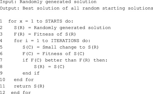
One type of local search algorithm is the Hill-Climbing algorithm (HCA). This algorithm generates a random solution and makes small changes to the solution to increase the fit to target data. The HCA is greedy as it only accepts a solution better than its current state. As a result, the HCA can get stuck firstly, in a local maximum, which is a peak higher than each of its neighbours but lower than the global maximum; secondly, in a flat local maximum, which is a local maximum that has many solutions and is difficult for the algorithm to navigate; and finally, at a shoulder, which is a flat region of space that is neither a local or global maximum (Russell and Norvig, 2013). To overcome such sticking points the HCA can be modified into a stochastic Random-Restart Hill-Climbing algorithm (RRHCA) by defining a number of times to re-run the whole program. The final solution is the best of all runs.

The goals of the fitting were (Objective 1) to reproduce the order of the time taken from the first 5 deaths to a peak for daily new cases, (Objective 2) to reproduce the order of the height of the peaks for daily new cases, and (Objective 3) combining Objective 1 and Objective 2. Fitting was performed in all three cases using target driven optimisation employing Random Restart Hill Climbing. RRHC was used for parameter optimisation with code developed in Python which called Spike. This Python program automatically optimises input parameters to better represent the target data. Using this approach, the three objectives were investigated for West Europe10.

First, optimisation was performed for the order of peak new daily infections (PNDI). Each country was given a unique letter and a string produced to represent the order of peaks, for example: France = A, Spain = B, if Spain peaked first the string was “BA”, else it was “AB”. The fitness function for Objective 1 was achieved by encoding the required country order for peak time as a ten character string, and minimising the Levenshtein distance between the target string and the corresponding string representing the order of peaks obtained from the model. Results are given in Supplementary Table S2. A smaller distance symbolises model predictions to be closer to the observed data, and the RRHC algorithm searched for country specific and inter-country infection parameters that reduced the distance measure for this objective and the two below.

Secondly, optimisation was performed for the magnitude of PNDI by minimising the result of Eq. 4. The measure produces a normalised value between 0 and 1, where 0 represented a perfect fit between target and modelled data, and 1 the worst possible fit, see Supplementary Table S3. Finally, for Objective 3, optimisation was performed for both the order and magnitude of PNDI. The distance measure used was a combination of the LD, and the measure in Objective 2, Eq. 5. The distance measure produces a normalised value between 0 and 1, where 0 represented a perfect fit between modelled and predicted data, and 1 the worst fit. Order and magnitude were given equal weight; see infection rates in Supplementary Table S4, and travel rates in Supplementary Table S5.

${\mathrm{d}\mathrm{i}\mathrm{s}\mathrm{t}\mathrm{a}\mathrm{n}\mathrm{c}\mathrm{e}}_{\mathrm{M}}=\frac{|\frac{{\mathrm{T}\mathrm{a}\mathrm{r}\mathrm{g}\mathrm{e}\mathrm{t}}_1-{\mathrm{M}\mathrm{o}\mathrm{d}\mathrm{e}\mathrm{l}}_1}{\mathrm{M}\mathrm{a}\mathrm{x}\left({\mathrm{T}\mathrm{a}\mathrm{r}\mathrm{g}\mathrm{e}\mathrm{t}}_1,{\mathrm{M}\mathrm{o}\mathrm{d}\mathrm{e}\mathrm{l}}_1\right)}|+|\frac{{\mathrm{T}\mathrm{a}\mathrm{r}\mathrm{g}\mathrm{e}\mathrm{t}}_2-{\mathrm{M}\mathrm{o}\mathrm{d}\mathrm{e}\mathrm{l}}_2}{\mathrm{M}\mathrm{a}\mathrm{x}\left({\mathrm{T}\mathrm{a}\mathrm{r}\mathrm{g}\mathrm{e}\mathrm{t}}_2,{\mathrm{M}\mathrm{o}\mathrm{d}\mathrm{e}\mathrm{l}}_2\right)}|+\cdots +|\frac{{\mathrm{T}\mathrm{a}\mathrm{r}\mathrm{g}\mathrm{e}\mathrm{t}}_n-{\mathrm{M}\mathrm{o}\mathrm{d}\mathrm{e}\mathrm{l}}_n}{\mathrm{M}\mathrm{a}\mathrm{x}\left({\mathrm{T}\mathrm{a}\mathrm{r}\mathrm{g}\mathrm{e}\mathrm{t}}_n,{\mathrm{M}\mathrm{o}\mathrm{d}\mathrm{e}\mathrm{l}}_n\right)}|}{n}(4)$

${\mathrm{d}\mathrm{i}\mathrm{s}\mathrm{t}\mathrm{a}\mathrm{n}\mathrm{c}\mathrm{e}}_{\mathrm{M}+\mathrm{O}}=\frac{{\mathrm{d}\mathrm{i}\mathrm{s}\mathrm{t}\mathrm{a}\mathrm{n}\mathrm{c}\mathrm{e}}_{\mathrm{M}}+\frac{LD}{n}}{2}(5)$

Pseudo code for RRHCA:

The Levenshtein distance (Levenshtein, 1966) between two strings a,b (of length ∣a∣ and ∣b∣ respectively) is given by lev_a,b(∣a∣, ∣b∣), where

$le{v}_{a,b}\left(i,j\right)=\left\{\begin{array}{cc}\mathit{max}\left(i,j\right)\hfill & \text{If}\min \left(i,j\right)=0\hfill \\ \mathit{min}\hfill & \left\{\begin{array}{c}le{v}_{a,b}=\left(i-1,j\right)+1\hfill \\ le{v}_{a,b}=\left(i,j-1\right)+1,\hfill & \text{otherwise}\hfill \\ le{v}_{a,b}=\left(i-1,j-1\right)+1_{\left(a_i\ne b_j\right)}\hfill \end{array}\right.\hfill \end{array}\right.$

where $1_{(a_i\ne b_j)}$ is the indicator function equal to 0 when a_i = b_j and equal to 1 otherwise. A normalised edit distance between two strings can be computed by

$lev\text{\_}nor{m}_{a,b}=\frac{le{v}_{a,b}}{\mathit{max}\left(\mid a\mid ,\mid b\mid \right)}$

3.4 Data Analytics

3.4.1 Supervised Analytics Via Linear Temporal Logic and Simulative Model Checking

Model checking permits us to determine if a model fulfils given properties specified in temporal logics, e.g., probabilistic linear-time temporal logic PLTL (Donaldson and Gilbert, 2008). Here we employ the simulative model checker MC2 (Donaldson and Gilbert, 2008) over time series traces of behaviours generated by simulation of epidemic and pandemic models. Our simulation platforms (Snoopy, Marcie, Spike) not only support the checking of time series behaviours of (uncoloured/coloured) places/compartments but also of (uncoloured/coloured) transitions/events, for example, Infect, Recover and Travel, or derived measures over both (observers). All of these can be subsumed under the general term observables.

The basic element of any temporal logic is the Atomic Proposition (AP) which is part of a property without temporal operators. The syntax of PLTL is:

φ ⩴ Xφ | Gφ | Fφ | φUφ | φRφ | φ ∨ φ | φ ∧ φ | ¬φ | φ → φ | AP

AP ⩴ AP ∨ AP | AP ∧ AP | ¬AP | AP → AP |z = z | z ≠ z | z > z | z ≥ z | z < z | z ≤ z | true | false

z ⩴ z + z | z − z | z ∗ z | z/z | ≪x≫ | d (≪x≫) | max (≪x≫) | Int | Real

Where ≪x≫ is the name of any observable in the simulation output, Int is any integer number, Real is any real number, and d is the differential operator.

The temporal operators are:

• Next (X)—The property must hold true in the next time point.

• Globally (G)—The property must hold true always in the future.

• Finally (F)—The property must hold true sometime in the future.

• Until (U)—The first property must hold true until the second property holds true.

• Release (R)—The second property can only ever not hold true if the first property becomes true.

When checking small models with few variables, it is possible to check the properties of specific observables, for example, that of infectious in a simple SIR model. However, when checking larger models with many observables, for example P₄₈SIR-S₁₀, we run model checking for a set of observables against a library of PLTL properties, and employ meta-variables indicated by double angle brackets in our queries, to be substituted one by one by all observables in the set:

P ≥1[G(≪x≫>10)]which “Holds for any observable whose value is always greater than 10”, which in turn could be generalised to a general pattern “x is always greater than some threshold”.

A library of appropriate property patterns, provided in the Supplementary Material, allows us to categorise all model observables into (not necessarily disjunctive) sets fulfilling the individual property patterns. Example patterns include

1) Always zero. When applied to places, this indicates that a place has never been initialised to a value greater than zero, and that it never participates in the progress of the model. For transitions it indicates those which are never active, indicating that they are part of the network that is always dead.

P ≥ 1[G(≪x≫= 0)], which is equivalent to P ≥ 1 [¬F(≪x≫ ≠ 0)]

2) At some point greater than zero, and eventually zero Places which have some marking, and then hold a zero value at then end of the simulation; transitions with changing activity and finally a steady state of zero activity.

P ≥ 1[F(d(≪x≫) ≠ 0) ∧ F(G(≪x≫ = 0 ∧ d(≪x≫) = 0))]

3) Activity peaks and falls:

$P\ge 1\left[\right.[F(d(\ll x\gg )>0)\wedge (d(\ll x\gg )>0UG(d(\ll x\gg )<0))]\left.\right]$

4) Activity peaks and falls, then steady state:

$\mathit{P}\ge 1\left[\right.[\mathit{F}(\mathit{d}(\ll \mathit{x}\gg )>0)\wedge \left(\right.\mathit{d}(\ll \mathit{x}\gg )>0\mathit{U}$

$(\mathit{F}(\mathit{d}(\ll x\gg )<0\wedge G(\mathit{d}(\ll \mathit{x}\gg )<0\mathit{U}\mathit{G}(\mathit{d}(\ll \mathit{x}\gg ))=0)))]\left.\right]$

5) At least one peak:

P ≥1[F((d(≪x≫)>0) ∧ F((d(≪x≫) < 0)))]

6) At least two peaks:

$\mathit{P}\ge 1\left[\right.[\mathit{F}((\mathit{d}(\ll \mathit{x}\gg )>0\wedge \mathit{F}((\mathit{d}\ll \mathit{x}\gg )<0)\wedge \mathit{F}((\mathit{d}(\ll \mathit{x}\gg )>0)\wedge \mathit{F}((\mathit{d}\ll \mathit{x}\gg )<0)))\left.))]\right)\left.\right)\left.\right]$

We have applied this to P_ChinaSIR, and discovered some provinces with multiple peaks in Infectious when the infection was initiated in Hubei province (the capital of which is Wuhan), due to their geographical placement, see Figure 10.

3.4.2 Unsupervised Analytics

Out of the rich choice available for unsupervised analytics, we use the following three methods; clustering, bar charts and correlation matrices.

Clustering is a method of creating groups where objects in one group are very similar and distinct from other groups (Gan et al., 2020). In particular, agglomerative hierarchical cluster analysis was performed, which sequentially combines individual elements into larger clusters until all elements are in the same cluster. Time-series cluster analysis was performed on the Infectious compartment in non-fitted Europe10 (Supplementary Figure S11) and non-fitted Europe48 (Supplementary Figure S12), where the infection was started in all locations. The distance between time-series traces of Infectious compartments for each country was computed using Euclidean distance and a distance matrix was constructed. Clustering was performed using the complete link method, which takes the largest distance between clusters to construct a dendrogram.

Exploratory data analysis involves using graphs and summary statistics to explore data; this was exploited largely by plotting model outputs for visualisation to ascertain whether or not the models were behaving as expected. The bar chart in Supplementary Figure S5 was produced using simulation data exported as CSV files, and generated in Excel.

Correlation matrices were computed to assess model behaviour in more depth and was used to validate both unfitted and fitted models. Non-fitted models were simulated several times with the infection starting in a different location, and then with all locations infected. The magnitude and timing of peak infections were detected for all simulations and combined into a single data frame. For the P₁₀SIR fitted model, the best result from the RRHCA optimisation was taken, and peak and timing of peaks were detected. Data were loaded into R and real-world data on country population density, country size, and the number of borders a country had were joined. Correlations between variables were computed to determine the parameters that were closely linked to higher numbers of infections. The correlation matrix was then plotted to visualise and statistical significance determined at p < 0.05. Non-significant correlations were displayed with a black cross. For details see Supplementary Table S6 and Supplementary Figures S8–S10.

3.5 Hardware and Software Requirements

3.5.1 Hardware

A standard computer with a Windows, Mac or Linux operating system (preferably 64-bit). The minimum RAM required is 8 GB; depending on the size of the constructed model, more memory may be needed. More heavy simulation experiments take advantage of multiple cores.

3.5.2 Software

The research reported in this paper has been achieved by help of the PetriNuts platform, which is also required to reproduce the results. The platform comprises several tools, which can be downloaded from http://www-dssz.informatik.tu-cottbus.de/DSSZ/Software. All these tools can be installed separately, are free for non-commercial use, and run on Windows, Linux, and Mac OS.

• Snoopy (Heiner et al., 2012) is a Petri net editor and simulator supporting various types of hierarchical (coloured) Petri nets, including all Petri net classes used in this paper, with an automatic conversion between them. Snoopy supports several data exchange formats, among them the Systems Biology Markup Language (SBML, level 1 and 2). For communication within the PetriNuts platform, Snoopy reads and writes ANDL (Abstract Net Description Language) and CANDL (Coloured ANDL) files, and writes simulation traces (places, transitions, observers) as CSV files. The ODEs induced by a $\mathcal{CPN}$ or $\mathcal{CPN}$^C can be exported to LaTeX, as plain text, or be written to be read by Octave, Matlab, or ERODE (Cardelli et al., 2017; Cardelli et al., 2021). Snoopy’s proprietary file format uses XML technology; default file extensions indicate the net class (i.e., pn, spn, cpn, colpn, colspn, colcpn). A Snoopy2LATEX generator supports documentation.

• Patty (Schulz, 2008) is a lightweight JavaScript to support Petri net animation (token flow) in a web browser; it does not require any installation on the user’s site. Patty reads (uncoloured) Petri nets in Snoopy’s proprietary format. All uncoloured Petri nets given in this paper can be animated in a purely qualitative manner at https://www-dssz.informatik.tu-cottbus.de/DSSZ/Research/ModellingEpidemics.

• Charlie (Heiner et al., 2015) is an analysis tool of (uncoloured) Petri net models applying standard techniques of Petri net theory (including structural analysis, such as conservativeness, and invariant analysis), complemented by explicit CTL and LTL model checking. Charlie reads ANDL files, and writes some analysis results (invariants, siphons, traps) into files, to be read by Snoopy for visualisation; for details see (Blätke et al., 2015).

• Marcie (Heiner et al., 2013) is a Model checker for qualitative Petri nets and $\mathcal{SPN}$, and their coloured counterparts; it combines exact analysis techniques gaining their efficiency by symbolic data structures (IDD) (Heiner et al., 2016) with approximative analysis techniques building on fast adaptive uniformization (FAU) and parallelized stochastic simulation (Gillespie, tau leaping, delta leaping). It supports CTL, CSL and PLTLc model checking. Marcie reads ANDL and CANDL files, and writes stochastic simulation traces (places, transitions, observers) as CSV files.

• Spike (Chodak and Heiner, 2019) is a command line tool for reproducible stochastic, continuous and hybrid simulation experiments of large-scale (coloured) Petri nets. Spike reads a couple of file formats, among them are SBML, ANDL and CANDL, and writes simulation traces (places, transitions, observers) as CSV files.

Snoopy, Marcie and Spike share a library of simulation algorithms, comprising four stochastic simulation algorithms (besides Gillespie’s exact SSA, three approximative algorithms) and a couple of stiff/unstiff solvers for continuous simulation; some of them use the external library SUNDIAL CVODE (Hindmarsh et al., 2005). See (Chodak and Heiner, 2019) for a quick reference.

• MC2 (Donaldson and Gilbert, 2008) is a Monte Carlo Model Checker for LTLc and PLTLc, operating on stochastic, deterministic, and hybrid simulation traces or even wetlab data, given as CSV files. We use MC2 to analyse deterministic and stochastic traces generated by Snoopy or Spike.

Additionally, we recommend the use of several third-party tools for post-processing of simulation traces.

• R—3.6.2 and R Studio—Version 1.1.463, with packages dplyr 0.8.5, ggplot2 3.3.0, openxlsx 4.1.4, corrplot 0.84, RColorBrewer 1.1-2, dtwclust 5.5.6, reshape2 1.4.3.

• Python—Version 3.6.5 and Visual Studio Code—1.42.1, used for

• RRHCA (Random Restart Hill Climbing) using packages pandas 1.1.0, Levenshtein 0.12.0, and packages pre-installed with Python: os, time, random, datetime.

• Python Web Scraper, used to collect COVID-19 Data, using packages urllib3 1.25.10, requests 2.24.0, lxml 4.5.2, bs4 0.0.1.

• Excel 16.40

4 Discussion

4.1 Model Engineering

Model engineering is in general the science of designing, constructing and analysing computational models. We have previously discussed this concept in the context of biological models (Heiner and Gilbert, 2013; Blätke et al., 2015), and the principles are equally applicable to epidemic and pandemic models. Major objectives of this approach are the sound reusability of models, and the reproducibility of their simulation and analysis results, both being facilitated by the use of colour in Petri nets. In terms of the models presented in this paper, we employ an approach based on orthogonal extensions of the basic SIR model, enabling robust step-wise model development. Examples include the extension of epidemic SIR models to pandemic models in a reusable manner, where models can be scaled by modifying stratification colour sets, or adjusted to different geographies by merely replacing the related colour definitions. More specifically, model engineering in this context comprises three aspects: engineering model structure, spatial aspects, and rates.

4.2 Engineering Model Structure

We exploit the concept of colour as supported in coloured Petri nets, which facilitates parameterised repetition of model components, as for example, required to encode stratified populations. This enables modelling at a higher level of abstraction akin to principles in high level programming languages. Abstraction generally reduces design errors in large and complex models, but can introduce some implementation errors due to misunderstanding of the coloured annotations.

This calls for robust model validation before entering the simulation phase. With increasing model size, this can hardly be accomplished by visual inspection only. Petri nets offer structural analysis techniques for this purpose. For example, all the models presented in this paper are by construction covered by P-invariants, and most models are also conservative. Both properties can be easily checked using our Petri net analysis tool Charlie (see Section 3 for details). Besides this, animation of discrete Petri nets offers the option to play with a net in order to follow the token flow, suggested as an early check to reveal design faults. All our models can be animated with Snoopy; animation of coloured models involves stepwise partial unfolding of the transition to fire next. Uncoloured models can additionally be animated within a web browser using Patty.

Our use of colour enables us to construct multilevel models in a sound manner. Specifically they encode two levels, the lower one being based on an SIR or its extensions, and the upper level comprising a network of geographical connections, resulting in a metapopulation model (Brauer, 2017). The models are multiscale in terms of distances at the upper level; regarding time, we assume that geographical connections, i.e., travel, occur at much lower rates than infections in the lower level SIR components.

4.3 Engineering Spatial Aspects

The crucial difference between epidemic and pandemic models is the notion of space and connectivities permitting population movement and hence the geographic transmission of disease. Our approach which is based on colour and associated functions enables the encoding, for example, of set operators. This in turn facilitates model design based directly on abstract representations of spatial relationships as graphs. Modification of geographical relationships then merely involves modifying the corresponding graph at the coloured high level, rather than attempting to change the expanded and more complex unfolded low level. This all occurs within one smooth coherent framework of coloured Petri nets, implemented seamlessly in our PetriNuts platform.

Petri nets can be designed in a graphical or textual way, depending on personal preferences. A combination of both is also possible; for example, designing the Petri net structure graphically and writing all colour-related definitions using CANDL; Supplementary Material for details.

4.4 Engineering Rates

The increase in model size results in an increase both in the number of kinetic parameters that need to be fitted, as well as an increase in the complexity of their interdependencies. Our paper is a methodology paper, and parameter fitting has been included as an illustration of what can be done with our approach.

In this paper we have discussed models where the rate constants are fixed for the entirety of a simulation. Modelling lockdown situations, however, requires that rate constants are changed dynamically during a simulation run. The imposition of lockdown measures which are driven by social disease control policies effectively diminishes the infection rate constant, and likewise lifting of the measures increases this value. These changes are typically event driven, in response to changing ${\mathcal{R}}_t$ values for example. We have recently extended the Spike simulator to include event-driven triggers, which enables the modelling of these control measures, for example, Figure 11—lockdown only, Figure 12—lockdown followed by unlock. The methodology enables the imposition of changes in an some incremental manner, in order to better represent the transitional nature of the uptake of lockdown measures in practice. In more general terms modelling features such as the dynamic modification of rate constants is a step towards self-adaptable models.

FIGURE 11

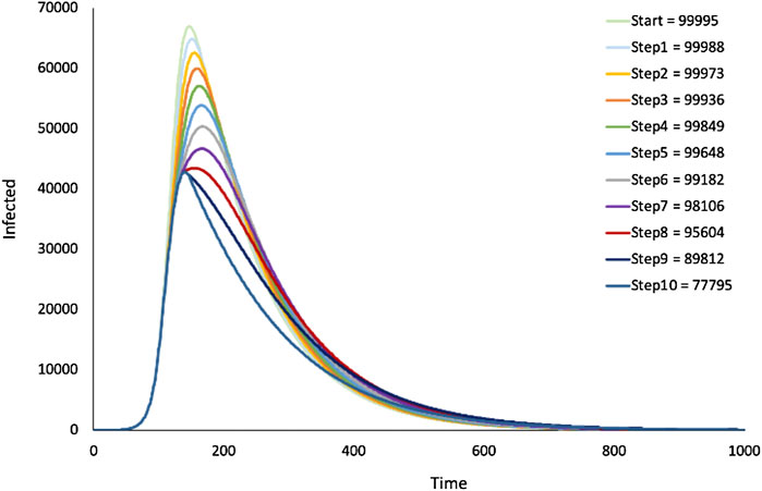
FIGURE 11. SIR model—Dynamic change of infection rates: lockdown. Output from the SIR model in Figure 1 where infection rates were stepwise decremented during simulation. Figure legend shows cumulative infections for different number of decrements.

FIGURE 12

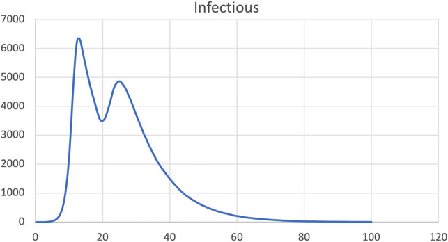
FIGURE 12. SIR model, dynamic change of infection rate increased back to pre-intervention level at time step 20.

Data Availability Statement

The original contributions presented in the study are included in the article/Supplementary Material, further inquiries can be directed to the corresponding author.

Author Contributions

MH and DG contributed equally to the paper by developing together the modelling approach and simulative model checking approach, as well as writing the main part of the paper. SC constructed the Europe map models, and performed data analytics on the behaviour of the models, including parameter optimisation as part of a Masters project.

Conflict of Interest

The authors declare that the research was conducted in the absence of any commercial or financial relationships that could be construed as a potential conflict of interest.

Publisher’s Note

All claims expressed in this article are solely those of the authors and do not necessarily represent those of their affiliated organizations, or those of the publisher, the editors and the reviewers. Any product that may be evaluated in this article, or claim that may be made by its manufacturer, is not guaranteed or endorsed by the publisher.

Acknowledgments

We would like to thank George Assaf, Jacek Chodak, Robin Donaldson, Mostafa Herajy, Ronny Richter, Christian Rohr, Martin Schwarick and many students at the Brandenburg Technical University, Cottbus, Germany for developing the PetriNuts platform.

Supplementary Material

The Supplementary Material for this article can be found online at: https://www.frontiersin.org/articles/10.3389/fsysb.2022.861562/full#supplementary-material

References

Adam, D. (2020). A Guide to R - the Pandemic's Misunderstood Metric. Nature 583, 346–348. doi:10.1038/d41586-020-02009-w

PubMed Abstract | CrossRef Full Text | Google Scholar

Amparore, E. G., Beccuti, M., Castagno, P., Franceschinis, G., Pennisi, M., and Pernice, S. (2021). “Multiformalism Modeling and Simulation of Immune System Mechanisms,” in 2021 IEEE International Conference on Bioinformatics and Biomedicine (BIBM) (IEEE), 3259–3266. doi:10.1109/bibm52615.2021.9669796

CrossRef Full Text | Google Scholar

Anand, N., Sabarinath, A., Geetha, S., and Somanath, S. (2020). Predicting the Spread of COVID-19 Using $$SIR$$ Model Augmented to Incorporate Quarantine and Testing. Trans. Indian Natl. Acad. Eng. 5, 141–148. doi:10.1007/s41403-020-00151-5

CrossRef Full Text | Google Scholar

Aràndiga, F., Baeza, A., Cordero-Carrión, I., Donat, R., Martí, M. C., Mulet, P., et al. (2020). A Spatial-Temporal Model for the Evolution of the COVID-19 Pandemic in Spain Including Mobility. Mathematics 8, 1677. doi:10.3390/math8101677

CrossRef Full Text | Google Scholar

Bajardi, P., Poletto, C., Ramasco, J. J., Tizzoni, M., Colizza, V., and Vespignani, A. (2011). Human Mobility Networks, Travel Restrictions, and the Global Spread of 2009 H1N1 Pandemic. PloS one 6, e16591. doi:10.1371/journal.pone.0016591

PubMed Abstract | CrossRef Full Text | Google Scholar

Balabdaoui, F., and Mohr, D. (2020). Age-stratified Model of the COVID-19 Epidemic to Analyze the Impact of Relaxing Lockdown Measures: Nowcasting and Forecasting for Switzerland. medRxiv 10 (1), 1–12. doi:10.1101/2020.05.08.20095059

CrossRef Full Text | Google Scholar

Balcan, D., Colizza, V., Gonçalves, B., Hu, H., Ramasco, J. J., and Vespignani, A. (2009). Multiscale Mobility Networks and the Spatial Spreading of Infectious Diseases. Proc. Natl. Acad. Sci. U.S.A. 106, 21484–21489. doi:10.1073/pnas.0906910106

PubMed Abstract | CrossRef Full Text | Google Scholar

Balcan, D., Gonçalves, B., Hu, H., Ramasco, J. J., Colizza, V., and Vespignani, A. (2010). Modeling the Spatial Spread of Infectious Diseases: The GLobal Epidemic and Mobility Computational Model. J. Comput. Sci. 1, 132–145. doi:10.1016/j.jocs.2010.07.002

PubMed Abstract | CrossRef Full Text | Google Scholar

Beccuti, M., Capra, L., De Pierro, M., Franceschinis, G., Follia, L., and Pernice, S. (2019). “A Tool for the Automatic Derivation of Symbolic ODE from Symmetric Net Models,” in 2019 IEEE 27th International Symposium on Modeling, Analysis, and Simulation of Computer and Telecommunication Systems (MASCOTS) (IEEE), 36–48. doi:10.1109/mascots.2019.00015

CrossRef Full Text | Google Scholar

Beccuti, M., Fornari, C., Franceschinis, G., Halawani, S. M., Ba-Rukab, O., Ahmad, A. R., et al. (2015). From Symmetric Nets to Differential Equations Exploiting Model Symmetries. Comput. J. 58, 23–39. doi:10.1093/comjnl/bxt111

CrossRef Full Text | Google Scholar

Blätke, M. A., Heiner, M., and Marwan, W. (2015). “BioModel Engineering with Petri Nets,” in Algebraic and Discrete Mathematical Methods for Modern Biology (Elsevier), 141–192. chap. 7. doi:10.1016/B978-0-12-801213-0.00007-1

CrossRef Full Text | Google Scholar

Brauer, F. (2017). Mathematical Epidemiology: Past, Present, and Future. Infect. Dis. Model. 2, 113–127. doi:10.1016/j.idm.2017.02.001

PubMed Abstract | CrossRef Full Text | Google Scholar

Breitling, R., Gilbert, D., Heiner, M., and Orton, R. (2008). A Structured Approach for the Engineering of Biochemical Network Models, Illustrated for Signalling Pathways. Brief. Bioinform. 9, 404–421. doi:10.1093/bib/bbn026

PubMed Abstract | CrossRef Full Text | Google Scholar

Cardelli, L., Perez-Verona, I. C., Tribastone, M., Tschaikowski, M., Vandin, A., and Waizmann, T. (2021). Exact Maximal Reduction of Stochastic Reaction Networks by Species Lumping. Bioinformatics 37, 2175–2182. doi:10.1093/bioinformatics/btab081

PubMed Abstract | CrossRef Full Text | Google Scholar

Cardelli, L., Tribastone, M., Tschaikowski, M., and Vandin, A. (2017). “ERODE: A Tool for the Evaluation and Reduction of Ordinary Differential Equations,” in Tools and Algorithms for the Construction and Analysis of Systems (Springer), 310–328. LNCS 10206. doi:10.1007/978-3-662-54580-5_19

CrossRef Full Text | Google Scholar

Castagno, P., Pernice, S., Ghetti, G., Povero, M., Pradelli, L., Paolotti, D., et al. (2020). A Computational Framework for Modeling and Studying Pertussis Epidemiology and Vaccination. BMC bioinformatics 21, 344. doi:10.1186/s12859-020-03648-6

PubMed Abstract | CrossRef Full Text | Google Scholar

Chen, Y., Yan, M., and Xiang, Z. (2014). Transmission Dynamics of a Two-City SIR Epidemic Model with Transport-Related Infections. J. Appl. Maths. 2014, 1–12. doi:10.1155/2014/764278

CrossRef Full Text | Google Scholar

Chodak, J., and Heiner, M. (2019). “Spike - Reproducible Simulation Experiments with Configuration File Branching,” in Proc. CMSB 2019. Editors L. Bortolussi, and G. Sanguinetti (Springer), 315–321. 11773 of LNCS/LNBI. doi:10.1007/978-3-030-31304-3_19

CrossRef Full Text | Google Scholar

Colizza, V., and Vespignani, A. (2008). Epidemic Modeling in Metapopulation Systems with Heterogeneous Coupling Pattern: Theory and Simulations. J. Theor. Biol. 251, 450–467. doi:10.1016/j.jtbi.2007.11.028

PubMed Abstract | CrossRef Full Text | Google Scholar

De la Sen, M., Ibeas, A., Alonso-Quesada, S., and Nistal, R. (2017). On a New Epidemic Model with Asymptomatic and Dead-Infective Subpopulations with Feedback Controls Useful for Ebola Disease. Discrete Dyn. Nat. Soc. 2017, 1–22. doi:10.1155/2017/4232971

CrossRef Full Text | Google Scholar

Del Valle, S. Y., Hyman, J. M., and Chitnis, N. (2013). Mathematical Models of Contact Patterns between Age Groups for Predicting the Spread of Infectious Diseases. Math. Biosci. Eng. 10, 1475–1497. doi:10.3934/mbe.2013.10.1475

PubMed Abstract | CrossRef Full Text | Google Scholar

Donaldson, R., and Gilbert, D. (2008). “A Model Checking Approach to the Parameter Estimation of Biochemical Pathways,” in Proc. CMSB (Springer), 269–287. LNCS 5307. doi:10.1007/978-3-540-88562-7_20

CrossRef Full Text | Google Scholar

Edlund, S. B., Davis, M. A., and Kaufman, J. H. (2010). “The Spatiotemporal Epidemiological Modeler,” in Proceedings of the 1st ACM International Health Informatics Symposium (ACM), 817–820. doi:10.1145/1882992.1883115

CrossRef Full Text | Google Scholar

Gan, G., Ma, C., and Wu, J. (2020). Data Clustering: Theory, Algorithms, and Applications. SIAM.

Google Scholar

Gao, Q., Gilbert, D., Heiner, M., Liu, F., Maccagnola, D., and Tree, D. (2013). Multiscale Modeling and Analysis of Planar Cell Polarity in the Drosophila Wing. Ieee/acm Trans. Comput. Biol. Bioinf. 10, 337–351. doi:10.1109/TCBB.2012.101

PubMed Abstract | CrossRef Full Text | Google Scholar

Genrich, H. J., and Lautenbach, K. (1981). System Modelling with High-Level Petri Nets. Theor. Comput. Sci. 13, 109–135. doi:10.1016/0304-3975(81)90113-4

CrossRef Full Text | Google Scholar

Gilbert, D., Heiner, M., Ghanbar, L., and Chodak, J. (2019). Spatial Quorum Sensing Modelling Using Coloured Hybrid Petri Nets and Simulative Model Checking. BMC Bioinformatics 20. doi:10.1186/s12859-019-2690-z

PubMed Abstract | CrossRef Full Text | Google Scholar

Gilbert, D., Heiner, M., Liu, F., and Saunders, N. (2013). “Colouring Space - A Coloured Framework for Spatial Modelling in Systems Biology,” in Proc. Petri Nets 2013. Editors J. Colom, and J. Desel (Springer), 230–249. vol. 7927 of LNCS. doi:10.1007/978-3-642-38697-8_13

CrossRef Full Text | Google Scholar

Gillespie, D. T. (1976). A General Method for Numerically Simulating the Stochastic Time Evolution of Coupled Chemical Reactions. J. Comput. Phys. 22, 403–434. doi:10.1016/0021-9991(76)90041-3

CrossRef Full Text | Google Scholar

Giordano, G., Blanchini, F., Bruno, R., Colaneri, P., Di Filippo, A., Di Matteo, A., et al. (2020). Modelling the COVID-19 Epidemic and Implementation of Population-wide Interventions in Italy. Nat. Med. 26, 855–860. doi:10.1038/s41591-020-0883-7

PubMed Abstract | CrossRef Full Text | Google Scholar

Goel, R., and Sharma, R. (2020). “Mobility Based Sir Model for Pandemics-With Case Study of Covid-19,” in 2020 IEEE/ACM International Conference on Advances in Social Networks Analysis and Mining (ASONAM) (IEEE), 110–117. doi:10.1109/asonam49781.2020.9381457

CrossRef Full Text | Google Scholar

Heffernan, J. M., Smith, R. J., and Wahl, L. M. (2005). Perspectives on the Basic Reproductive Ratio. J. R. Soc. Interf. 2, 281–293. doi:10.1098/rsif.2005.0042

PubMed Abstract | CrossRef Full Text | Google Scholar

Heiner, M., and Gilbert, D. (2013). Biomodel Engineering for Multiscale Systems Biology. Prog. Biophys. Mol. Biol. 111, 119–128. Online available 12-OCT-2012. doi:10.1016/j.pbiomolbio.2012.10.001

PubMed Abstract | CrossRef Full Text | Google Scholar

Heiner, M., Gilbert, D., and Donaldson, R. (2008). Petri Nets for Systems and Synthetic Biology. Springer, 215–264. vol. 5016 of LNCS. doi:10.1007/978-3-540-68894-5_7

CrossRef Full Text | Google Scholar

Heiner, M., and Gilbert, D. (2011). How Might Petri Nets Enhance Your Systems Biology Toolkit. Springer, 17–37. vol. 6709 of Lecture Notes in Computer Science. doi:10.1007/978-3-642-21834-7_2

CrossRef Full Text | Google Scholar

Heiner, M., Herajy, M., Liu, F., Rohr, C., and Schwarick, M. (2012). “Snoopy - a Unifying Petri Net Tool,” in Proc. Petri Nets 2012 (Springer), 398–407. vol. 7347 of LNCS. doi:10.1007/978-3-642-31131-4_22

CrossRef Full Text | Google Scholar

Heiner, M., Rohr, C., and Schwarick, M. (2013). “MARCIE - Model Checking and Reachability Analysis Done effiCIEntly,” in Proc. PETRI NETS 2013. Editors J. Colom, and J. Desel (Springer), 389–399. vol. 7927 of LNCS. doi:10.1007/978-3-642-38697-8_21

CrossRef Full Text | Google Scholar

Heiner, M., Rohr, C., Schwarick, M., and Streif, S. (2010). “A Comparative Study of Stochastic Analysis Techniques,” in Proc. 8th International Conference on Computational Methods in Systems Biology (CMSB 2010) (ACM digital library), 96–106. doi:10.1145/1839764.1839776

CrossRef Full Text | Google Scholar

Heiner, M., Rohr, C., Schwarick, M., and Tovchigrechko, A. A. (2016). “MARCIE's Secrets of Efficient Model Checking,” in Transactions on Petri Nets and Other Models of Concurrency (ToPNoC) XI (Springer), 286–296. LNCS 9930. doi:10.1007/978-3-662-53401-4_14

CrossRef Full Text | Google Scholar

Heiner, M., Schwarick, M., and Wegener, J.-T. (2015). “Charlie - an Extensible Petri Net Analysis Tool,” in Proc. PETRI NETS 2015. Editors R. Devillers, and A. Valmari (Springer), 200–211. vol. 9115 of LNCS. doi:10.1007/978-3-319-19488-2_10

CrossRef Full Text | Google Scholar

Heiner, M. (2009). “Understanding Network Behavior by Structured Representations of Transition Invariants,” in Natural Computing Series (Springer), 367–389. doi:10.1007/978-3-540-88869-7_19

CrossRef Full Text | Google Scholar

Hethcote, H. W. (2000). The Mathematics of Infectious Diseases. SIAM Rev. 42, 599–653. doi:10.1137/s0036144500371907

CrossRef Full Text | Google Scholar

Hindmarsh, A. C., Brown, P. N., Grant, K. E., Lee, S. L., Serban, R., Shumaker, D. E., et al. (2005). Sundials. ACM Trans. Math. Softw. 31, 363–396. doi:10.1145/1089014.1089020

CrossRef Full Text | Google Scholar

Ismail, A., Herajy, M., Atlam, E., and Heiner, M. (2020). A Graphical Approach for Hybrid Simulation of 3D Diffusion Bio-Models via Coloured Hybrid Petri Nets. Model. Simulation Eng. 2020, 4715172. 14 pages. doi:10.1155/2020/4715172

CrossRef Full Text | Google Scholar

Jensen, K., and Kristensen, L. M. (2009). Coloured Petri Nets: Modelling and Validation of Concurrent Systems. Springer.

Google Scholar

Levenshtein, V. I. (1966). Binary Codes Capable of Correcting Deletions, Insertions, and Reversals. Soviet Phys. doklady 10, 707–710.

Google Scholar

Liu, F., Heiner, M., and Gilbert, D. (2019). Coloured Petri Nets for Multilevel, Multiscale and Multidimensional Modelling of Biological Systems. Brief. Bioinform. 20, 877–886. Published: 03 November 2017. doi:10.1093/bib/bbx150

PubMed Abstract | CrossRef Full Text | Google Scholar

Longini, I. M. (1988). A Mathematical Model for Predicting the Geographic Spread of New Infectious Agents. Math. Biosciences 90, 367–383. doi:10.1016/0025-5564(88)90075-2

CrossRef Full Text | Google Scholar

Mahmood, I., Arabnejad, H., Suleimenova, D., Sassoon, I., Marshan, A., Serrano-Rico, A., et al. (2020). FACS: a Geospatial Agent-Based Simulator for Analysing COVID-19 Spread and Public Health Measures on Local Regions. J. Simulation, 1–19. doi:10.1080/17477778.2020.1800422

CrossRef Full Text | Google Scholar

Murata, T. (1989). Petri Nets: Properties, Analysis and Applications. Proc. IEEE 77, 541–580. doi:10.1109/5.24143

CrossRef Full Text | Google Scholar

Nandi, A., and Allen, L. J. S. (2019). Stochastic Two-Group Models with Transmission Dependent on Host Infectivity or Susceptibility. J. Biol. Dyn. 13, 201–224. doi:10.1080/17513758.2018.1538462

PubMed Abstract | CrossRef Full Text | Google Scholar

Oka, T., Wei, W., and Zhu, D. (2020). A Spatial Stochastic SIR Model for Transmission Networks with Application to COVID-19 Epidemic in China. SSRN J. doi:10.2139/ssrn.3675213

CrossRef Full Text | Google Scholar

Pârvu, O., Gilbert, D., Heiner, M., Liu, F., Saunders, N., and Shaw, S. (2015). Spatial-temporal Modelling and Analysis of Bacterial Colonies with Phase Variable Genes. ACM Trans. Model. Comput. Simul. 25, 1–25. doi:10.1145/2742546

CrossRef Full Text | Google Scholar

Prem, K., Liu, Y., Russell, T. W., Kucharski, A. J., Eggo, R. M., Davies, N., et al. (2020). The Effect of Control Strategies to Reduce Social Mixing on Outcomes of the COVID-19 Epidemic in Wuhan, China: a Modelling Study. The Lancet Public Health 5 (5), e261–e270. doi:10.1016/s2468-2667(20)30073-6

PubMed Abstract | CrossRef Full Text | Google Scholar

Russell, S., and Norvig, P. (2013). Artificial Intelligence: Pearson New International Edition: A Modern Approach. Pearson Higher Ed.

Google Scholar

Rvachev, L. A., and Longini, I. M. (1985). A Mathematical Model for the Global Spread of Influenza. Math. biosciences 75, 3–22. doi:10.1016/0025-5564(85)90064-1

CrossRef Full Text | Google Scholar

Sattenspiel, L., and Powell, C. (1993). Geographic Spread of Measles on the Island of Dominica, West Indies. Hum. Biol. 65, 107–129.

PubMed Abstract | Google Scholar

Sattenspiel, L., and Dietz, K. (1995). A Structured Epidemic Model Incorporating Geographic Mobility Among Regions. Math. Biosciences 128, 71–91. doi:10.1016/0025-5564(94)00068-b

CrossRef Full Text | Google Scholar

Schulz, K. (2008). An Extension of the Snoopy Software to Process and Manage Petri Net Animations (In German). BTU Cottbus, Dep. of CS. Bachelor thesis.

Google Scholar

Schwarick, M., and Heiner, M. (2009). “CSL Model Checking of Biochemical Networks with Interval Decision Diagrams,” in Proc. 7th International Conference on Computational Methods in Systems Biology (CMSB 2009) (Springer), 296–312. vol. 5688 of LNCS/LNBI. doi:10.1007/978-3-642-03845-7_20

CrossRef Full Text | Google Scholar

Schwarick, M., Rohr, C., Liu, F., Assaf, G., Chodak, J., and Heiner, M. (2020). “Efficient Unfolding of Coloured Petri Nets Using Interval Decision Diagrams,” in Proc. PETRI NETS 2020. Editors T. C. R Janicki, and N. Sidorova (Cham: Springer), 324–344. vol. 12152 of LNCS. doi:10.1007/978-3-030-51831-8_16

CrossRef Full Text | Google Scholar

Soliman, S., and Heiner, M. (2010). A Unique Transformation from Ordinary Differential Equations to Reaction Networks. PLoS ONE 5, e14284. doi:10.1371/journal.pone.0014284

PubMed Abstract | CrossRef Full Text | Google Scholar

Van den Broeck, W., Gioannini, C., Gonçalves, B., Quaggiotto, M., Colizza, V., and Vespignani, A. (2011). The GLEaMviz Computational Tool, a Publicly Available Software to Explore Realistic Epidemic Spreading Scenarios at the Global Scale. BMC Infect. Dis. 11, 37–14. doi:10.1186/1471-2334-11-37

PubMed Abstract | CrossRef Full Text | Google Scholar

van den Driessche, P. (2017). Reproduction Numbers of Infectious Disease Models. Infect. Dis. Model. 2, 288–303. doi:10.1016/j.idm.2017.06.002

PubMed Abstract | CrossRef Full Text | Google Scholar

Wilson, E. B., and Worcester, J. (1945). The Law of Mass Action in Epidemiology. Proc. Natl. Acad. Sci. U.S.A. 31, 24–34. doi:10.1073/pnas.31.1.24

PubMed Abstract | CrossRef Full Text | Google Scholar