1
Institute for Theoretical Biology, Department of Biology, Humboldt Universität, Berlin, Germany
2
Bernstein Center for Computational Neuroscience, Berlin, Germany
3
Centro Atómico Bariloche and Instituto Balseiro, San Carlos de Bariloche, Argentina
Various classes of neurons alternate between high-frequency discharges and silent intervals. This phenomenon is called burst firing. To analyze burst activity in an insect system, grasshopper auditory receptor neurons were recorded in vivo for several distinct stimulus types. The experimental data show that both burst probability and burst characteristics are strongly influenced by temporal modulations of the acoustic stimulus. The tendency to burst, hence, is not only determined by cell-intrinsic processes, but also by their interaction with the stimulus time course. We study this interaction quantitatively and observe that bursts containing a certain number of spikes occur shortly after stimulus deflections of specific intensity and duration. Our findings suggest a sparse neural code where information about the stimulus is represented by the number of spikes per burst, irrespective of the detailed interspike-interval structure within a burst. This compact representation cannot be interpreted as a firing-rate code. An information-theoretical analysis reveals that the number of spikes per burst reliably conveys information about the amplitude and duration of sound transients, whereas their time of occurrence is reflected by the burst onset time. The investigated neurons encode almost half of the total transmitted information in burst activity.
Tonic and burst firing encode different aspects of the sensory world. Specifically, in thalamic relay cells, burst firing has been reported as more efficient in signal detection than tonic firing (Grubb and Thompson, 2005
; Lesica et al., 2006
; Sherman 2001
) and more reliable to repeated presentations of the same stimulus (Alitto et al., 2005
; Denning and Reinagel, 2005
). Tonic firing, in turn, seems to be well suited for encoding the detailed evolution of time-varying stimuli. Similar results have been obtained in electric fish (Chacron et al., 2004
; Metzner et al., 1998
; Oswald et al., 2004
).
Various studies have compared the stimuli that trigger isolated spikes with those that induce burst firing (Alitto et al., 2005
; Denning and Reinagel, 2005
; Eggermont and Smith, 1996
; Grubb and Thompson, 2005
; Metzner et al., 1998
; Oswald et al., 2004
; Reinagel et al., 1999
). In these comparisons bursts were taken as a single type of event, without further discrimination between different burst variants. However, bursts may also encode stimuli in a graded manner (Kepecs et al., 2001
; Oswald et al., 2007
; Kepecs
et al., unpublished). Bursts with different numbers of spikes can thus act as compact code-words. Indeed, in neurons from various sensory systems the number n of spikes within a burst correlates with particular properties of the external stimulus, such as the orientation of a drifting sine-wave grating (DeBusk et al., 1997
) and the slope or the amplitude of visual contrast changes (Kepecs et al., 2001
; Kepecs
et al., unpublished).
Here, we examine the role of bursts in grasshopper auditory receptor cells. When stimulated with time-dependent acoustic signals, these neurons fire high-frequency bursts that are triggered by stimulus deflections of specific intensity and duration. We quantify the amount of information encoded by a burst code and characterize the stimulus features represented by bursts of different duration. Receptor cells, however, do not generate bursts in response to constant or step stimuli (Gollisch and Herz, 2004
; Gollisch et al., 2002
), indicating that bursts can result from a non-trivial interplay between external stimuli and intrinsic dynamics. Our analysis leads to the following conclusions: (a) burst-firing constitutes a prominent feature in the neural code of the investigated auditory neurons, (b) representing neural responses by intra-burst spike counts n allows one to estimate the amount and type of transmitted information in a straightforward manner, (c) the correspondence between code-words and the stimulus features that they represent may be readily explored with burst-triggered averages. Most importantly, (d) burst coding is a key element in the transmission of time-varying stimuli even for cells that are not intrinsic bursters.
Electrophysiology and Stimulus Design
All experiments were conducted on adult Locusta migratoria. The animal’s metathoracic ganglion and nerve were exposed. Spikes were recorded intracellularly from the axons of auditory receptors located in the tympanal nerve, see Rokem et al. (2006)
for details. The auditory stimulus was played from a loudspeaker located ipsilateral to the recorded neurons, at 30 cm from the animal. Thirty-seven receptor cells were recorded, from 23 animals. Each cell was tested with two or more stimuli, resulting in 132 data sets in total (one data set, or session, corresponds to one cell in one stimulus condition). The experimental protocol complied with German law governing animal care.
Each experiment began with a measurement of the “best” or “preferred” sound frequency of the receptor, that is, the frequency of a sinusoidal acoustic wave for which the threshold of the cell is lowest. To that end, the animal was exposed to a pure tone between 3 and 20 kHz. The frequency that induced spiking with minimal stimulus amplitude was selected as the best frequency of the cell, and the minimal intensity inducing spiking constituted the threshold sTH. The mean threshold across the population was 58 dB (SD 14 dB). Mimicking behaviorally relevant stimuli, the sound signals used for further analysis consisted of amplitude modulated (AM) carrier sine waves whose frequency matched the cell’s best frequency. The AM signal was white up to a certain cutoff frequency and had a Gaussian amplitude distribution with a given standard deviation (see Figure 1
, for an example). A detailed explanation of the stimulus construction may be found in Machens et al. (2001)
. Increasing the standard deviation results in more pronounced variations of the amplitude modulations. By varying the cutoff frequency, instead, the temporal scale of the stimulus excursions is altered, with higher cutoff frequencies corresponding to more rapid amplitude deflections.
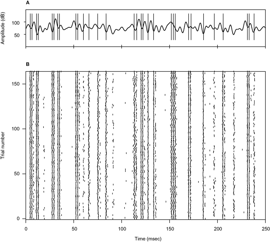
Figure 1. Example of an acoustic stimulus and neural response from a single recording session. (A) Wavy line: random amplitude modulation (AM signal) of a carrier sine wave. The standard deviation of the AM signal is 12 dB, its cutoff frequency is 200 Hz. Vertical lines: elicited spikes. The cell generates either isolated spikes, or stereotyped patterns consisting of 2–3 spikes separated by a short interval. (B) Raster plot corresponding to the recording shown in (A), for 165 repetitions. Both the timing of individual spikes and the number of spikes in each pattern appear as reliable features, fairly well preserved throughout the different trials.
Different receptors vary in their cellular properties, resulting in different response characteristics. To identify the effect of the stimulus on the response (in spite of the cell-to-cell variability) each cell was presented with two stimuli. One stimulus was the same for all cells: a Gaussian amplitude distribution with 6 dB standard deviation and 200 Hz cutoff frequency. The other signal could be one of six different stimulation protocols. In four of them, the standard deviation of the amplitude modulation was fixed at 6 dB, and the cutoff frequency was either 25, 100, 400 or 800 Hz. In the other two protocols, the cutoff frequency was fixed at 200 Hz, whereas the standard deviation was set to either 3 or 12 dB.
Given that the mean firing rate has a strong effect on the transmitted information (Borst and Haag, 2001
), the mean stimulus was adjusted to obtain an average firing rate of about 100 Hz. The resulting firing rates had a mean of 113 Hz (SD = 16 Hz), and they did not show any significant variation in the different stimulus conditions, as assessed by a one-way ANOVA (p = 0.58). In addition, given that information measures require stationary recordings, we only kept those sessions where the trial-to-trial SD of the firing rate was <35 Hz (the population average of this SD is 6 Hz). There were 86 out of 132 data sets that fulfilled these two conditions.
Once the carrier frequency and mean stimulus amplitudes were determined, N repetitions of each stimulus were presented, with N ranging between 98 and 503 (average 172), depending on how long the recording could be sustained. Each stimulus lasted for 1 s, though in all results presented here, the first 200 msec of each trial were discarded, to avoid the initial transient response, where fast adaptation processes take place. Different trials were separated by pauses of 700 msec to prevent slow adaptation effects (Benda and Herz, 2003
).
Burst Identification
Neural responses were preprocessed to decide which cells had a natural tendency to generate bursts, and in these cases, to identify the bursts. With such a procedure, all spikes should either be classified as isolated spikes (a 1-spike burst), or be grouped into bursts of two or more discharges (an n-spikes burst). We therefore searched for a reliable criterion to establish a limit value of the inter-spike interval (ISI) separating pairs of consecutive spikes, such that all those pairs whose intervals lie below the limit be considered as part of the same burst, and all those that fall above the limit be classified as belonging to different bursts. Previous approaches (see, for example, Kepecs and Lisman, 2003
; Metzner et al., 1998
; Oswald et al., 2007
; Reich et al., 2000
; Reinagel et al., 1999
) have determined the value of the limiting ISI from the shape of the ISI distribution. In this work, we have taken an alternative approach, based on the shape of the correlation function.
If a cell shows a tendency to generate bursts, not all intervals between pairs of spikes are equally probable. We evaluated the correlation function (also called autocorrelation) of each cell discretizing the time axis in Nb bins, each of duration δt = 0.1 msec. The spike train ρ(t) is represented as a binary string such that, for any given t, ρ(t) is either equal to 1/δt or to 0, depending on whether or not a spike is fired inside [t, t + δt]. The post-stimulus-time histogram rs(t) = <ρ(t)> is the trial average of ρ(t). The mean firing rate  is defined as the temporal average of rs(t). The correlation function of the spike train is
is defined as the temporal average of rs(t). The correlation function of the spike train is
where the horizontal bar represents both trial average and temporal averages over t. A large, positive value of Cs(τ) indicates that there is a high probability of finding two spikes separated by a time lag τ, irrespective of whether there are other spikes in between or not. If Cs is near 0, this probability is roughly the one to be expected from the mean firing rate of the cell. If Cs(τ) is large and negative, the probability that two spikes be separated by an interval τ is low.
Figure 2
shows typical responses from four cells. The left column depicts the response to 15 identical stimulus presentations to each cell. The correlation functions Cs(τ) are presented in the middle column, and for comparison, the ISI distributions corresponding to the same spike trains are given in the right column. In cell Figure 2
A, both the correlation function and the ISI distribution exhibit a prominent peak. This peak constitutes a clear signature of the tendency of the cell to fire action potentials about every 3 msec, as can be seen in the raster plot. The width of this peak can be easily estimated from either the correlation function or the ISI distribution, since in both cases the peak is limited on its right-hand side by a minimum whose location can be clearly identified (marked by the arrow). In such cases, the limiting value of the ISI defining burst firing may be set as that ISI where the minimum is located. However, there are more complicated cases, too. The following examples (Figures 2
B,C) depict two cells that also tend to burst, as shown by the raster plots. In Figure 2
B, there are frequent doublets or triplets of spikes, whereas in Figure 2
C, each burst typically contains between 6 and 10 spikes. The width of the first peak of the correlation function can be determined quite easily. However, the temporal span of the corresponding peak in the ISI distribution is much more difficult to determine, since the right tail of the peak decreases essentially monotonically. Moreover, the ISI distribution of cell Figure 2
C completely misses the structure of peaks in the corresponding correlation function.
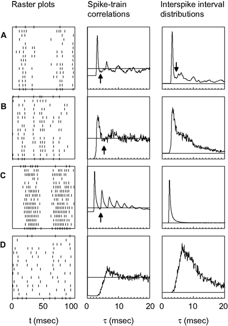
Figure 2. Examples of neural responses (left), and the corresponding spike train correlation functions (middle) and ISI distributions (right). The four rows of panels depict different cells. In the middle and right panels, the horizontal line represents the zero level of the respective quantity. The arrows indicate the limiting ISI defining burst generation. The upper three cells (A, B, C) show a tendency to fire action potentials separated by a fairly constant ISI, as seen from the raster plots. The correlation functions allow a clear estimation of the limiting ISI needed to define bursts, even in cases where this is not possible using ISI distributions (B and C). The last cell (D) lacks well defined time scales for intra-burst and inter-bursts ISIs.
ISI distributions reflect only the interval between two consecutive spikes, whereas correlation functions include intervals between any two spikes. Hence, ISI distributions often show an almost exponential decay, that conceals some of the structure exhibited by the correlation functions. For this reason, we shall base our choice of the limiting ISI defining bursts on the behavior of the correlation function, and not on the ISI distribution. We have verified that the two methods give different results only when applied to cells that have a tendency to generate long bursts (including more than five spikes). In these cases, if our method is applied to the ISI distributions, it fails to detect the minimum ISI separating inter-bursts and intra-bursts intervals. The correlation function, instead, shows a clear multi-peak structure. The example cell Figure 2
D is once again simple. It has no tendency to generate bursts, and consequently, both the correlation function and the ISI distribution reveal rather broad, unspecific structures.
We stipulated that a cell be classified as bursting if its correlation function contained a first peak that was limited on the right side by a minimum that could be considered significantly different from the maximum. Below, an ad-hoc method to determine the separability of the maximum is provided. In addition, the maximum was required to lie below τ = 5 msec, and the minimum to the right of the maximum should be located below 1.25 times the inverse cutoff frequency of the AM signal. These criteria reject fluctuations in the correlation function arising from limited sampling, as could be any of the many small troughs observed in Figure 2
B, and avoid a misclassification where two consecutive spikes are generated by two consecutive fluctuations in the stimulus.
To assess whether the correlation function contained a separable first peak (in the above sense), an ad-hoc statistical analysis was performed. To that end, the expected error of the correlation function was estimated, for all times τ. Notice that Cs(τ) can be interpreted as an average (see Eq. 1). The error bar Δ of an average estimated from N samples reads , where σ is the standard deviation of the data to be averaged (Barlow, 1999
). The population mean of the temporal average of this estimated error was 3.4% (SD 1.5%) of the total span of Cs(τ) (that is, the difference between the maximum and the minimum). Two values of Cs(τ) and Cs(τ′) were classified as significantly different if they differed in more than the sum of their estimated error bars. This is an ad-hoc procedure, since it is based on the assumption that the estimation errors of Cs(τ) are independent for different times τ, which may not be the case. However, we have checked that in all cases, the limiting ISI identified with our method could be easily detected visually.
, where σ is the standard deviation of the data to be averaged (Barlow, 1999
). The population mean of the temporal average of this estimated error was 3.4% (SD 1.5%) of the total span of Cs(τ) (that is, the difference between the maximum and the minimum). Two values of Cs(τ) and Cs(τ′) were classified as significantly different if they differed in more than the sum of their estimated error bars. This is an ad-hoc procedure, since it is based on the assumption that the estimation errors of Cs(τ) are independent for different times τ, which may not be the case. However, we have checked that in all cases, the limiting ISI identified with our method could be easily detected visually.Not all cells, and not all stimuli, gave rise to correlation functions that contained a separable first peak (for example, Figure 2
D shows a non-bursting cell). Whenever the peak could be separated, the domain of the peak was defined as the interval between 0 and the position of the first minimum after the peak. In the remaining cases, the domain of the peak was defined as 0. All spikes in a neural response were assigned to sequences containing 1, 2, or more action potentials, hereafter called bursts of intra-burst spike count n or, more compactly, n-bursts. An n-burst was defined as the set of consecutive spikes whose ISIs fell within the domain of the first peak of the correlation function. In those sessions where this peak was not separable, all spikes were classified as 1-bursts, or, as we shall also call them, as isolated spikes.
The present method of identifying bursts differs from other criteria employed previously (Gourévitch and Eggermont, 2007
; Kepecs and Lisman, 2003
; Metzner et al., 1998
; Oswald et al., 2007
; Reich et al., 2000
) in two aspects. First, we use ad-hoc statistical techniques to prevent small fluctuations, caused by limited sampling, from hampering burst identification. Second, our approach is based on the correlation function, and not the ISI distribution. Both quantities are closely related under various conditions. In fact, for stationary renewal processes, the correlation function can be derived through convolution from the ISI distribution (Perkel et al., 1967
). A clear minimum of the correlation function can therefore be expected if the standard deviation of the ISI distribution is sufficiently smaller than the mean ISI. On the other hand, it is more convenient to identify bursting neurons by analyzing their correlation function. If the minimum in the correlation function is significant, its location provides the value of the limiting ISI that is needed to segment a given spike train into sequences of bursts.
Model Neurons
To assess whether complex neural dynamics are needed to obtain burst-like responses to time-dependent stimuli, we modeled the firing probability density rs(t) of a measured cell as a simple, threshold-linear function of the stimulus, with added refractoriness, namely

where s*(t) is defined as
s(t) is the AM signal extending throughout the interval [0, T],  is the temporal mean value of s*(t), h(τ) stands for the filter of the cell, tlast is the time at which the previous spike was fired, tref is the refractory period, sTH is the threshold of the cell, and Θ is Heaviside step function [Θ(t) = 0, if t < 0, and Θ(t) = 1, if t ≥ 0). Note that the stimulus is thresholded before it is filtered. Gollisch and Herz (2005)
disclosed the detailed processes involved in sound transduction. They showed that the input current entering the auditory receptor after acoustic stimulation is a non-linear (quadratic) function of the sound intensity. Thus, low stimulus amplitudes are ineffective in generating ionic currents, whereas large intensities have an amplified effect. In Eq. 2, for simplicity, we have assumed that the non-linearity involved in sound transduction is a thresholding operation, representing ionic channels that only open when the AM signal surpasses a certain characteristic value that we can actually measure. This model, although simplified, correctly reproduces the threshold-linear dependence of firing frequency vs. stimulus amplitude that we have observed experimentally for the stimulus intensities in this study. In Eq. 2, the current is further filtered to represent the capacitive properties of the cell membrane (Gollisch and Herz, 2005
). For each modeled cell, the linear filter h(τ) was obtained from a cross-correlation analysis of the spike train and s*(t) (Koch and Segev, 1998
), whereas the refractory period tref was defined as the minimal ISI of the cell, and sTH was measured experimentally (see Electrophysiology and Stimulus Design). Finally, spike generation was modeled as a Poisson process with time-dependent rate rs(t). Note that the model contains no free fit parameters.
is the temporal mean value of s*(t), h(τ) stands for the filter of the cell, tlast is the time at which the previous spike was fired, tref is the refractory period, sTH is the threshold of the cell, and Θ is Heaviside step function [Θ(t) = 0, if t < 0, and Θ(t) = 1, if t ≥ 0). Note that the stimulus is thresholded before it is filtered. Gollisch and Herz (2005)
disclosed the detailed processes involved in sound transduction. They showed that the input current entering the auditory receptor after acoustic stimulation is a non-linear (quadratic) function of the sound intensity. Thus, low stimulus amplitudes are ineffective in generating ionic currents, whereas large intensities have an amplified effect. In Eq. 2, for simplicity, we have assumed that the non-linearity involved in sound transduction is a thresholding operation, representing ionic channels that only open when the AM signal surpasses a certain characteristic value that we can actually measure. This model, although simplified, correctly reproduces the threshold-linear dependence of firing frequency vs. stimulus amplitude that we have observed experimentally for the stimulus intensities in this study. In Eq. 2, the current is further filtered to represent the capacitive properties of the cell membrane (Gollisch and Herz, 2005
). For each modeled cell, the linear filter h(τ) was obtained from a cross-correlation analysis of the spike train and s*(t) (Koch and Segev, 1998
), whereas the refractory period tref was defined as the minimal ISI of the cell, and sTH was measured experimentally (see Electrophysiology and Stimulus Design). Finally, spike generation was modeled as a Poisson process with time-dependent rate rs(t). Note that the model contains no free fit parameters.Information Theoretical Analysis
Brenner et al. (2000)
have calculated the mean amount of information IE(1) transmitted by an event E, where E is a pre-defined combination of spikes and silent intervals. Such an event is either present or absent, in one given trial, at one particular time. When the event E is a single spike
where the event rate rs(t) is the probability density of a spike at time t (Brenner et al., 2000
; Rieke et al., 1997
), and  is the temporal average of rs(t). In Eq. 3, the upper index (1) denotes the mean information transmitted by each event. Notice that IE(1) is proportional to the dissimilarity between the spiking probability density rs(t) and a uniform density , as measured by the Kullback–Leibler divergence (Cover and Thomas, 1991
).
is the temporal average of rs(t). In Eq. 3, the upper index (1) denotes the mean information transmitted by each event. Notice that IE(1) is proportional to the dissimilarity between the spiking probability density rs(t) and a uniform density , as measured by the Kullback–Leibler divergence (Cover and Thomas, 1991
).We now extend this analysis to encompass events that are not just binary (present or absent), but appear in one of several possible alternatives. In our case, a burst may contain 0, 1, .. or n spikes. For each stimulus stretch s extending during the time interval [t − t0, t], the cell generates a response in the time bin [t, t + δt] that may either be “no spike” (n = 0), or the initiation of an n-burst (n > 0). The length of the interval t0 is assumed to be sufficiently large as to contain all structures in the stimulus that are causally related to the response of the neuron at time t. The mutual information Iδt between stimuli and n-bursts within [t, t + δt] is (Cover and Thomas, 1991
)
where P(s) is the prior probability of the stimulus segment s, P(n|s) is the probability of response n whose first spike falls in the interval [t, t + δt] conditional to the stimulus s, and

is the prior probability of response n. In Eqs 4 and 5 the sums in s include all possible stimulus stretches spanning the interval [t − t0, t], each one of them with its probability P(s).
If δt is sufficiently small, then for all n > 0 the probability P(n|s) may be approximated by rn(s)δt, where rn(s) is the n-burst rate conditional on the stimulus s, and is proportional to the fraction of trials where an n-burst was initiated in [t, t + δt], in response to stimulus s. Similarly,  . Replacing these expressions in Eq. 4 results in
where

If the stimulus is stationary, all possible stimulus stretches s will eventually be found as time goes by, each one of them with a frequency that is proportional to P(s). Therefore, for long enough stimuli, averaging over s with the probability distribution P(s) may be replaced by time averaging. That is,
where now the n-burst rate rn(t) is expressed as a function of time, and
Equation 7 provides a first estimate of the mutual information between stimuli and responses in a short interval [t, t + δt]. The aim is now to extend this result to the whole response interval [0, T], which can be thought of a concatenation of small intervals [0, δt], [δt, 2δt], … [(k − 1)δt, kδt], where k = T/δt. This extension, however, can only be done if the response in one time interval does not depend on the response in another time interval. Consider the response vector 
 , where n(τ) represents the number of spikes contained in the burst whose first spike fell in [τ, τ + δt] (n = 0 means that the cell remained silent). If different time bins are independent, then
, where n(τ) represents the number of spikes contained in the burst whose first spike fell in [τ, τ + δt] (n = 0 means that the cell remained silent). If different time bins are independent, then
This means that that responses in different time bins are independent from one another, given a fixed stimulus history. Full independence of time bins, however, implies that the factorization of Eq. 8 should not only hold for each stimulus history, but also for the marginal probabilities
These quantities represent the probability of the word  and the i-th bit n inside the word at any temporal location within the spike train. Then, if different time bins are independent, in addition to Eq. 8, we must also have
and the i-th bit n inside the word at any temporal location within the spike train. Then, if different time bins are independent, in addition to Eq. 8, we must also have
implying that independence also holds for arbitrary stimulus histories. When these two conditions are fulfilled, and given the additive properties of information (Cover and Thomas, 1991
), the mutual information I between stimuli and responses in [0, T] is the sum of the mutual information between stimuli and responses in each sub-interval [(j − 1)δt, jδt]. Hence,
where the last two equivalences serve as definitions of the average information In(1) transmitted by each single n-burst, and the information In transmitted by all the bursts of a given n, respectively. Finally, the information per unit time I′ (also called information rate), and the rates I′n are obtained by dividing the corresponding expressions in Eq. 10 by the total time interval T.
We emphasize that Eq. 10 is only valid under the independence assumption, that is, if Eqs 8 and 9 hold. In this work, we assume that all correlations in the spike train of third or higher order can be neglected. Under this approximation, different time bins are independent, if they are uncorrelated. This means that the probability distribution of a binary string  is well approximated by a Gaussian function
  , where
 . This approximation should hold both for strings
  starting at a fixed time t, and also for any time. The Pearson correlation coefficient between time bins
is well approximated by a Gaussian function , where . This approximation should hold both for strings starting at a fixed time t, and also for any time. The Pearson correlation coefficient between time bins
quantifies the correlations between n(t) and n(t + τ) for a fixed stimulus history, and hence may be used to test whether Eq. 8 is valid. In Eq. 11, n*(t) = n(t) − <n(t)>, and the angular brackets represent trial averages. In order to make Eq. 11 well defined even at times when the response of the neuron has no variability (that is, <[n*(t)]2> = 0 or <[n*(t + τ)]2> = 0), we set cb(t, τ) ≡ 0 if both the numerator and the denominator vanish.
In the absence of higher-order correlations, whenever cb(t, τ) ≈ 0 for all t and τ, one can assert that Eq. 8 holds. To assess whether burst identification succeeded in decreasing the correlations in the spike train, cb(t, τ) should be compared with a similar correlation coefficient cs(t, τ) calculated from a binary representation of the spike train including the whole collection of spikes. cs(t, τ) is defined by a formula analogous to Eq. 11, but with the integer variable n replaced by a binary variable indicating the presence or absence of a spike in each time bin. To quantify the total amount of correlations in a given domain t ∈[t1, t2] and t ∈[τ, τ′], we use the mean square value of the Pearson correlation coefficient [cb(t, τ) or cs(t, τ)] in the selected domain.
The Pearson correlation coefficient between n(t) and n(t + τ) for any stimulus history is
where the bar represents both a trial and a temporal (t) average. In the absence of higher-order correlations, whenever cb(τ) ≈ 0 for all τ, one can assert that Eq. 9 holds. To compare the correlations between bursts with the correlations between spikes, Eq. 12 should be compared with cs(t), defined by a formula analogous to Eq. 12, but with the integer variable n replaced by a binary variable representing individual spikes.
Estimation of Burst-Triggered Averages
The spike-triggered average (STA) was calculated as the mean stimulus preceding a spike, namely,
where s(t) is the time-dependent stimulus, N0 is the total number of spikes, and the sum ranges over all spike times t0. In every investigated cell, STA(τ) showed a pronounced peak. The time between the maximum of the peak and τ = 0 (spike generation) is the average latency between upward stimulus deflections and spike occurrences. As an extension, the n-burst triggered averages (nBTAs) were introduced to represent the mean stimulus preceding an n-burst (Kepecs and Lisman, 2003
; Lesica et al., 2006
; Oswald et al., 2007
), that is,

where now, the sum ranges over all times tn at which an n-burst begins (that is, the time of the first spike), and Nn is the total number of n-bursts. The time τn between the maximum of nBTA and τ = 0 (burst generation) is the average latency of the n-burst.
The nBTA at a particular τ is the arithmetical average of a collection of values, whose standard deviation reads
To determine whether the nBTAs corresponding to different n-values differed significantly, an ANOVA was conducted. The test was performed in the frequency domain, to avoid temporal correlations. The nBTA in the time interval ranging from −25 to +15 msec from burst generation was Fourier transformed and a two-way ANOVA was separately conducted on the real and imaginary parts of the frequency representation of the signal (since these constitute two comparisons, Bonferroni’s correction for multiple hypothesis testing was incorporated), with frequency band and the order of the burst as factors in the analysis. The null hypothesis was 1BTA = 2BTA = 3BTA = 4BTA. The corrected significance level was set at 0.01. Cells showing a significant difference (either as a main effect, or an interaction) were further tested in the time domain, to determine the intervals where the difference was observed. This was done using independent t-tests, for each point in time. In this case, the null hypothesis was that at time t, nBTA(t) differed from at least one of the other n′BTA(t), for any n′ ≠ n. In this analysis, n and n′ ranged between 1 and 4. Hence, to reject the null hypothesis for a given n and t, three comparisons with different n′-values are needed.
For n ≥ 2, we also compared the nBTAs with a combination of n 1BTAs interleaved with the same ISIs found in the real data. For every n-burst in the experimental data, we calculated the function

where the times ti indicate the location of each spike within the burst. Each n-burst, hence, produces a function fn(t). By averaging the fn(t) obtained for all bursts with the same spike count n, we calculated the averaged convolved 1BTA. We estimated the variability of the convolved 1BTA as the standard deviation of the averaged data. To test whether the real nBTA was significantly different from the reconstructed fn, we first carried out a two-way ANOVA. The null hypothesis was nBTA = fn in a time interval extending between the two minima at each side of the central maximum of the nBTA. To avoid temporal correlations, the comparisons were performed in Fourier space, testing real and imaginary parts separately. A Bonferroni correction for multiple comparisons was incorporated. The corrected significance level was set at 0.01. Cells showing a significant difference (either as a main effect or an interaction) where further tested in the time domain, to determine whether the difference was observed in an extended fraction of the time interval. This was done with an independent t-test, for each point in time. In this case, the null hypothesis was that at time t, nBTA(t) = fn(t). We reported the number of cells for which the null hypothesis was rejected in 70% of the times t within an interval extending between the two minima at each side of the central maximum of the nBTA. As a check, the whole procedure was also carried out replacing the 1BTA(t) in Eq. 15 with STA(t). Recall that the 1BTA is the average stimulus preceding 1-bursts, or isolated spikes. The STA, in turn, is the average stimulus preceding all action potentials in the spike train.
For completeness, we mention that the amount of jitter (Rokem et al., 2006
) is defined as the trial-to-trial standard deviation of the time of the first spike in a burst, and the average estimated error bar in jitter estimation is 0.2 msec.
Relating Burst Probabilities to the Height of Stimulus Excursions
To calculate the probability P(n|h) of obtaining a burst with n spikes after a stimulus deflection of maximal height h, we went through all local maxima of the stimulus, one at a time, and for each one we searched whether there was a burst in the response that could be associated with the maximum. This was done in the following way. Each n-burst in the response was first shifted backwards τn milliseconds. Next, for a given stimulus maximum located at time t0, we searched for (shifted) n-bursts inside a window [t0 − T, t0 + T], where T was the width of the most prominent peak of the STA of the whole collection of spikes (prior to burst identification). In other words, T was the interval where a given response can be expected to be correlated with a maximum in the stimulus. If within that interval no bursts were found, then the maximum located at t0 was said not to be associated with any response. If the first spike of an n-burst fell within the window, then the maximum in the stimulus was associated with that n-burst. If there was more than one burst inside the window, then a single burst was selected, by choosing that one whose first spike lay closest to t0. Next, if a given burst was associated to more than a single maximum, the closest maximum was assigned to the burst (and not the others).
This algorithm allows one to associate each maximum in the stimulus with either no response, or with an n-burst. Note, however, that so far we have no reason to claim that there is a causal connection between the maximum and the associated burst. In principle, given that we do not actually know what feature in the stimulus induces burst generation (it could be the height of the stimulus amplitude, the size of its derivative, the width of an upward excursion, and so forth) this association between stimuli and responses could represent no more than a completely arbitrary connection. Only if we can show that the association contains non-trivial features that would be unlikely between randomly connected events can we suspect that it could indeed contain some predictive value.
To reveal those features, we estimated P(n|h ∈ [h0 − Δh, h0 + Δh]), i.e., the probability of obtaining a burst of n spikes, given that the height of the stimulus maximum h fell in [h0 − Δh, h0 + Δh]. The width Δh was chosen as 5% of the span of values of h. P(n|h) is depicted in Figure 10
for an example cell. The partial segregation between the different curves shows that the height of the maximum h can tell something about the stimulus. Even though one still cannot guarantee a causal relationship between each maximum and its associated n-burst, this result ensures that the intra-burst spike count n provides information about the height of the stimulus deflection preceding it – not excluding that it may also provide information about other stimulus features.
Stimulus Characteristics Modulate Burst Probability
Depending on the characteristics of the ionic channels that compose the cellular membrane and temporal properties of their activation and inactivation variables, different neurons respond to the same stimulus with different firing patterns. In particular, some neurons have a tendency to alternate between periods of high-frequency discharges and silent intervals. This is called burst firing. The mathematics of burst firing has been studied extensively in the computational neuroscience literature (see, for example, Izhikevich, 2000
; Izhikevich and Hoppensteadt, 2004
; Wang and Rinzel, 1995
). Irrespective of the particular mechanisms underlying the generation of bursts, here we explore their role in the transmission of sensory information. To that end, we quantify the reliability with which bursts correspond to specific stimulus features.
In principle, the possibility to generate bursts would allow a neuron to construct a non-trivial temporal code, in which both the time at which the burst initiates and the number of spikes within a burst carry specific information. In order to assess whether this is the case in a classic insect model system (Gollisch and Herz, 2005
; Hill, 1983
; Machens et al., 2001
, 2005
; Römer, 1976
; Ronacher and Römer, 1985
; Sippel and Breckow, 1983
; von Helversen and von Helversen, 1994
), the activity of grasshopper auditory receptor neurons was recorded in vivo during acoustic stimulation. Figure 1
A depicts an example stimulus (wavy line), together with the elicited spikes (vertical lines). This cell sometimes generates isolated action potentials, whereas at other times it fires spike doublets or triplets. In this particular recording, responses typically appear after stimulus upstrokes with an delay of 3.4 msec, including both acoustic and axonal time lags. The data suggest that whereas fairly shallow stimulus excursions are followed by, at most, a single action potential, deflections that are more pronounced (either in height or in width) are often accompanied by short sequences of multiple spikes. Figure 1
B depicts the response of the same neuron to 165 identical repetitions of the stimulus. Clearly, the bursting pattern of this cell is highly reproducible across trials.
These observations suggest that short sequences of high-frequency firing appear with higher probability in response to particular types of stimulus deflections. This raises the question whether the probability of generating bursts depends on the statistical properties of the sound wave. We therefore calculated the correlation function Cs(τ) of the neural response (see Materials and Methods). The upper subpanels of Figure 3
show Cs for a sample cell that was tested with the whole set of stimuli (the middle and lower subpanels correspond to simulated data discussed later on). Increasing the standard deviation of the amplitude distribution (from Figure 3
A to D to G) results in correlation functions that exhibit progressively sharper peaks. This is the signature of a high probability of generating sequences of two or more spikes separated by a fairly constant ISI. Moreover, a somewhat rippled pattern can be observed in the right tail of the distribution in Figure 3
G. Decreasing the typical time scale of the stimulus fluctuations (going right from Figure 3
B to F) leads from multi-modal (Figure 3
B) to single-peaked (Figures 3
C,D) to increasingly shallower and broader correlation functions (Figures 3
E,F).
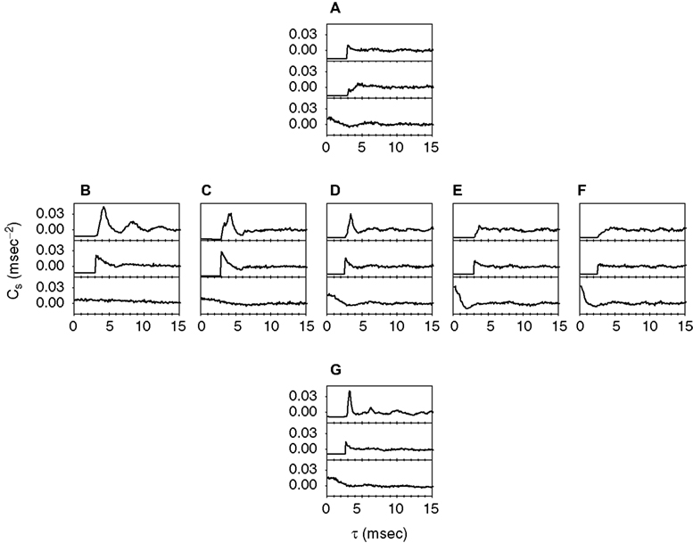
Figure 3. Spike-train correlations for a sample cell, and different stimulus conditions. Each sound stimulus consisted of a carrier wave with random Gaussian amplitude modulations that had a specific standard deviation and cutoff frequency. Upper subpanel: Experimental data. Middle subpanel: Threshold-linear model, with refractory period. Lower subpanels: Linear model. Neither model contains free fit parameters. Comparisons between the experimental data and the two models demonstrate that the combination of threshold and refractoriness captures the qualitative shape of the measured correlation functions. (A,D,G) Cutoff frequency = 200 Hz, and standard deviation 3 dB (A), 6 dB (D) and 12 dB (G). (B–F) Standard deviation = 6 dB, and cutoff frequency 25 Hz (B), 100 Hz (C), 200 Hz (D), 400 Hz (E), and 800 Hz (F).
Some correlation functions exhibit a pronounced first peak, easily distinguishable from the rest of the function (as in Figures 3
B–D,G), and spanning a finite and fairly clear temporal domain. In these cases, spikes are either closely packed with ISIs falling in the domain covered by the first peak, or they are loosely spread apart. The presence of a minimum between the first peak and the rest of the correlation function allows one to establish a natural upper limit to the range of preferred ISIs. Sometimes, this minimum is also present in the ISI distribution. In these cases, the cell has a tendency to fire with a typical “short” ISI that is clearly separated from other long ISIs. If the minimum only appears in the correlation function, but not in the ISI distribution, then the separation between these two time-scales cannot be achieved directly using the ISI distribution (see Materials and Methods). However, the tendency of the cell to fire sequences of three or more spikes with one typical ISI can still be clearly revealed by the correlation function. Finally, there are yet other cases where the correlation function is of an essentially unimodal nature, exhibiting no more than one broad, unspecific structure (Figures 3
A,E,F). In these cases, singling out a range of ISIs as “typical” would be questionable.
We define a burst as a sequence of spikes whose ISIs fall within the domain of the first peak of the correlation function, whenever such peak can be isolated (see Materials and Methods, for the statistical techniques used to assess the separability of this peak). This sequence of n spikes will be called a burst of intra-burst spike count n or, more compactly, an n-burst. In what follows, the temporal location of a burst is assigned to the time when its first spike occurs. Cells showing unimodal correlation functions are classified as non-bursting, and in the analysis below, all their spikes are considered as 1-bursts.
To underscore the differences between the n-burst code investigated in this study and the more conventional firing-rate codes, Figure 4
illustrates alternative representations of a sample spike train. Here, rate code is used whenever the stimulus is encoded by the firing rate, which is evaluated either instantaneously (as in Figure 4
C), or in extended time windows (Figures 4
D,E). In Figure 4
A, each vertical line represents an action potential of a cell that tends to generate high-frequency bursts with intra-burst ISIs of 2–3 msec. Figure 4
B depicts the n-burst representation of this spike train. Here, each time t is associated with an integer n that denotes the number of spikes contained in the burst starting at time t. The height of the vertical lines in Figure 4
B represents the value of n, and the grey arrows link each burst in Figure 4
A with the corresponding n-value in Figure 4
B. For comparison, three firing-rate codes are shown in Figures 4
FC–E. Figure 4
C illustrates the time-dependent instantaneous firing rate which is obtained from the sequence of inverse ISIs. Figures 4
D,E depict two alternative smoothed firing-rate representation. In Figure 4
D, each spike from Figure 4
A was convolved with a narrow bell-shaped kernel (Gaussian, 5 msec SD); in Figure 4
E, the SD is 20 msec.
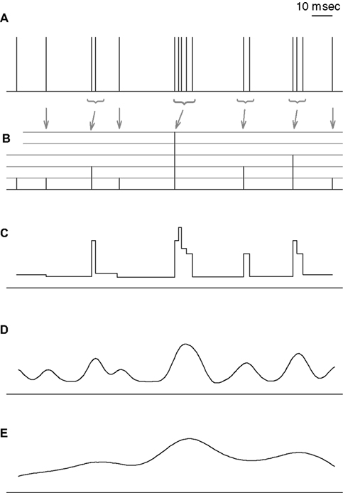
Figure 4. Graphical representation of different coding schemes. (A) Sample spike train. For this example, all consecutive spikes separated by <3 msec are considered as part of the same burst. (B) n-burst representation of the spike train. Each point in time t is associated with an integer n representing the number of spikes in a burst (if any) initiated at t. The height of the vertical lines represents n, and the arrows indicate the association between each burst in (A) and the corresponding n-value in (B). (C) Instantaneous firing rates, defined as inverse ISIs. (D) Smoothed-firing-rate representation, defined as the convolution of the spike train with a Gaussian function of 5 msec SD. (E) same as (D), but using a Gaussian function of 20 msec SD. Unlike traditional firing-rate codes (C–E), the n-burst code provides a reduced representation of the spike train – all ISIs shorter than the ISI cutoff used for burst definition are treated equally. In addition, the number of spikes in a burst can be directly read off from the n-burst representation whereas it is not locally available within firing-rate codes.
For invertible kernels, the firing-rate representations of Figures 4
C–E contain all information needed to reconstruct the full spike train in Figure 4
A. This is clearly not the case for the n-burst representation in Figure 4
B. Here, small variations of the intra-burst ISIs in Figure 4
A are no longer present. On the other hand, the number of spikes within a burst provided by the n-burst code is not locally available from the firing rate-codes in Figures 4
C–E. For these two reasons, the n-burst code is qualitatively different from a firing-rate code. The reduced information capacity of the n-burst code could severely limit its potential role for neural systems. It may, however, also provide a highly compact and thus most useful neural code. The present study aims at elucidating these alternatives.
Table 1
lists all stimulation protocols, together with a summary of the bursting properties of the investigated cell population. The fraction of bursting sessions, the percentage of isolated spikes (1-bursts), and the maximum n-value depend strongly on the standard deviation and cutoff frequency of the stimulus. Notice, however, that in all cases, isolated spikes are more frequent than any other burst of n > 1.
Different cells have different firing thresholds, and may therefore respond to the same stimulus with different mean firing rates. Both the burst statistics and the transmitted information depend on the firing rate. In order to be able to compare the results obtained for different cells, in all experiments reported here the mean stimulus amplitude was adjusted so as to obtain a mean firing rate near 100 Hz (see Materials and Methods). We also checked that the firing rate practically has no effect on the value of the limiting ISI defining bursts. More specifically, a 50 Hz increase in firing rate shifts the limiting ISI by <0.4 msec, which is comparable to its estimated error bar. The average intra-burst spike count n, in turn, shows an increase of <25%.
Stimulus statistics strongly influence the probability of generating specific bursts, as shown in Figure 5
. Here, the probability of an n-burst is depicted as a function of the cutoff frequency of the AM signal (Figure 5
A) and its standard deviation (Figure 5
B). The probability of generating isolated spikes is minimal for large amplitude fluctuations and cutoff frequencies around 100 Hz. For the sake of clarity, only data corresponding to n = 1, 2, and 3 are depicted.
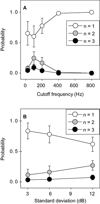
Figure 5. Population average of the probability of generating n-bursts, as a function of the stimulus cutoff frequency, for all SD = 6 dB stimuli (A) and as a function of standard deviation, for all stimuli with a cutoff frequency of 200 Hz (B). Error bars represent the standard deviation in the population. High-n-bursts appear most frequently for stimuli with large amplitude modulations and cutoff frequencies around 100 Hz. Stimulus properties thus have a noticeable influence on the probability of generating bursts.
In the present approach, a spike sequence is classified as an n-burst by analyzing the statistical properties of the response. There are no dynamical explanations in terms of specific ionic currents. Actually, though we lack a detailed characterization of the ionic currents involved in action potential generation, previous studies suggest that grasshopper receptors do not burst intrinsically; cells fire tonically for time-independent stimuli (Gollisch et al., 2002
) and do not show burst activity at the onset of step-like stimuli (Gollisch and Herz, 2004
). In addition, adaptation effects as well as spike-time variability can be explained on a quantitative level with models that do not contain intrinsic burst mechanisms (Benda et al., 2001
; Gollisch and Herz, 2004
; Schaette et al., 2005
). These results underscore that in the presence of time-dependent stimuli, even cells that do not burst by themselves may generate responses whose statistical properties are highly reminiscent of intrinsically bursting cells. Agüera y Arcas et al. (2003) and Keat et al. (2001)
present similar examples in simulated data. In these cases, burst-like responses arise as a consequence of the interplay between the dynamical properties of the neuron and particular temporal structures in the stimulus. To assess whether even cells with very simple dynamics can exhibit burst activity when driven by the proper stimulus, we modeled the time evolution of a threshold-linear Poisson neuron with added refractoriness (see Materials and Methods). The middle subpanels of Figure 3
depict the correlation functions for a model cell with the same filter characteristics, threshold and refractory period as the data shown in the upper subpanels (see Materials and Methods). These correlation functions exhibit similar qualitative features as those of the real cell. Recall that the modeled cells contain no free fit parameters. In both real (upper subpanels) and simulated (middle subpanels) data, the sessions that are classified as bursting (or non-bursting) coincide. When the analysis is extended to the whole population of cells, this agreement is observed in 86% of all sessions. Moreover, in those sessions where both real and simulated data are classified as bursting, the limiting ISI calculated with real and simulated data differ by <1 msec in 81% of the cases. However, the multiple peaks typically caused by slow stimuli (see, e.g., Figure 3
B) are only partially reproduced, indicating that the high temporal precision of subsequent spikes in multiple bursts is not captured by the simulations. Notice that refractoriness needs to be included in the model, otherwise the first peak in the correlation function shifts to τ = 0. Moreover, if the stimulus is not thresholded, the statistics of the modeled cell differs markedly from the real one. This is shown in the lower subpanels of Figure 3
, where the correlation function of a purely linear model with the same filter characteristics as the real cell is depicted. This model completely fails to capture the basic statistics of the experimental data, as can be judged from the absence of both the refractory period and the sharp peak in the correlation function.
Quantitative Description of the Information Transmitted by Bursts
Since the stimulus characteristics have a strong effect on the probability of burst generation, the number of spikes in a burst may encode specific stimulus aspects. If this hypothesis is indeed true, even a reduced burst representation of the spike train should carry information about the stimulating sound wave. The purpose of the present section is to translate this general idea into a quantitative information-theoretical analysis.
We represent the spike train as a sequence of non-negative integer numbers n, each number indicating the intra-burst spike count of the burst whose first spike falls in a small time window [t, t + δt] (see Figure 4
B, for an example). This representation should be compared to the more typical binary representation (Figure 4
A), where each digit in the sequence indicates the presence or absence of a spike in the relevant time bin. As shown in some of the examples of Figure 2
, the binary representation often contains strong temporal correlations. The very definition of an n-burst aims at bundling highly correlated spikes into a single burst event. Hence, the representation in terms of bursts necessarily reduces the statistical dependence between different time bins, as seen in Figure 6
. In Figure 6
A we show the Pearson correlation coefficient cs(t, τ) between spikes at times t and t + τ (see Materials and Methods), in an example cell. For comparison, Figure 6
B exhibits the correlation coefficient cb(t, τ) between bursts at times t and t + τ (see Materials and Methods), of the same spike train. For small τ-values, the plot in Figure 6
A shows a number of peaks, that are absent in Figure 6
B. For the cell shown in Figure 6
, the mean value of  averaged over all t ∈ [200, 990 msec] and τ ∈ [0, 10 msec] is 2.94 times larger than the corresponding mean of
  . The population average of this ratio on all bursting sessions is 2.89 (SD 1.49).
averaged over all t ∈ [200, 990 msec] and τ ∈ [0, 10 msec] is 2.94 times larger than the corresponding mean of . The population average of this ratio on all bursting sessions is 2.89 (SD 1.49).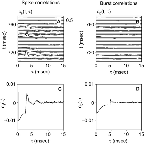
Figure 6. Pearson correlation coefficient for a sample cell. (A) Coefficient cs(t, τ) between spikes generated at times t and t + τ. The scale [also valid for (B)] is given in the upper-right corner. (B) Coefficient cb(t, τ) between bursts generated at times t and t + τ. (C,D) Coefficients cs(τ) and cb(τ) between spikes and bursts, respectively. In (A) and (C), a pronounced peak is seen for cs at around τ = 3 msec. In (C), there is also an initial negative plateau. These structures are markedly reduced in cb (B) and (D), underscoring that generic spikes are more correlated than classified bursts.
Figure 6
C depicts the Pearson correlation coefficient cs(τ), averaged both over all trials and all times t (see Materials and Methods). For comparison, the Pearson correlation coefficient cb(τ) obtained with an n-burst representation of the spike train is shown in Figure 6
D. The most prominent peak of cs appears markedly diminished in cb. This reduction demonstrates that bursts are more independent from each other than individual spikes.
Given the additive properties of information (Cover and Thomas, 1991
), if in one particular case, a collection of events can be shown to contain independent elements only, then the information transmitted by the collection is the sum of the information transmitted by the individual events. Figure 6
shows that the correlations between bursts are not strictly 0. Yet, if they can be assumed to be negligible, and if there are no higher order correlations, then the mutual information transmitted by the train of bursts can be easily calculated from the information in small time bins (see Materials and Methods, and Brenner et al., 2000
).
In Figure 7
, the information transmitted by burst firing is depicted for a sample cell, the left half of the figure corresponding to the experimental data, the right half to the threshold-linear model with refractoriness. Figure 7
A depicts the average information In(1) provided by each n-burst. The higher the intra-burst spike count n, the more informative the event is. To evaluate the significance of this trend, we fitted the data with a straight line, and evaluated the sign of the resulting slope, taking the estimated error bar of the fit into account. In the upper right corner of Figure 7
A, the value of the slope and its estimated error bar is indicated. Since n is dimensionless, slopes are also measured in bits. To assess how often In(1) was increasing at the population level, the analysis was repeated for all recorded bursting cells. All sessions had significantly positive slopes. Figure 7
B shows the distribution of slopes throughout the population. The average slope across the 59 bursting cells was 1.5 bits (SD 0.7 bits).
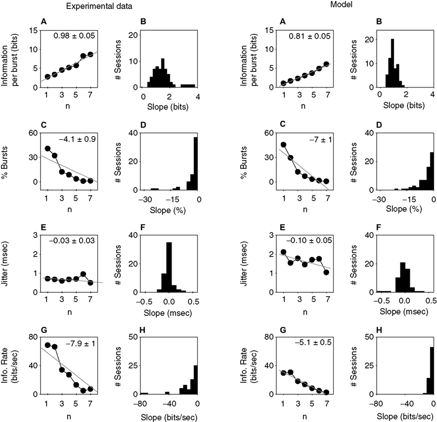
Figure 7. Information transmitted in burst firing. Left half of the figure: Experimental data. Right half of the figure: Threshold linear model with refractoriness. Left column: Data from the example cell of Figure 3
, with best linear fits. Their slopes are given in the upper-right corner, with their errors. Right column: Population data showing the distribution of slopes of the linear fits for the quantities of the left column. (A) Average information transmitted by each n-burst. The information transmitted per burst increases monotonously with n. (B) For all cells in the population, the information per burst increases with n. (C) Number of occurrences of each n-burst. The larger the intra-burst spike count n, the more rarely it appears. (D) For all cells in the population, low-n bursts appear more frequently than high-n bursts. (E) Mean amount of jitter of the first spike of each n-burst. (F) The population data demonstrate that for some cells, the amount of jitter is a slowly increasing function of n, whereas for other cells, it is decreasing. (G) Rate of transmitted information for all n-bursts. Although isolated spikes (n = 1) are the most frequent events [see (B)] a large fraction of the transmitted information is carried by bursts. (H) For all cells in the population, the information rate decreases with n. As shown by these data, the model captures the coding trends of the investigated neurons.
The information per burst In(1) is proportional to the dissimilarity between the time-dependent probability density rn(t) of an n-burst (see Materials and Methods) and a time-independent distribution of the same mean rate  . As such, it is large whenever rn(t) is a highly uneven function of time, almost always equal to 0, and only seldom exhibiting a sharp peak at a single, or at most a few, particular values of t. A burst is therefore a good candidate to transmit a large amount of information per event if it happens rarely (in each single trial), reliably (in a large fraction of the trials), and with high temporal accuracy. Figures 7
C,E depict the frequency of occurrence
. As such, it is large whenever rn(t) is a highly uneven function of time, almost always equal to 0, and only seldom exhibiting a sharp peak at a single, or at most a few, particular values of t. A burst is therefore a good candidate to transmit a large amount of information per event if it happens rarely (in each single trial), reliably (in a large fraction of the trials), and with high temporal accuracy. Figures 7
C,E depict the frequency of occurrence  and the amount of jitter of different n-bursts, respectively. Figure 7
C shows that high-n bursts occur seldom. This result was also observed in all other recorded cells: the frequency of occurrence always decreased significantly with n. The population data in Figure 7
D had an average slope of −2.6, with SD of 0.7. In Figure 7
E, the amount of jitter in the first spike of the burst is shown to be fairly constant with n. At the population level, in 80% of the bursting sessions the amount of jitter was roughly independent from n (the best linear fit had a slope that was not significantly different from 0). The remaining 20% showed a mild dependence, but with no uniform trend, as shown by the population data in Figure 7
F. The mean slope was −0.03 msec (SD 0.2 msec). The combined effect of an event probability that diminishes strongly with n (Figure 7
C) and a jitter that is fairly constant with n (Figure 7
E) results in an information per event In(1) that increases with n (Figure 7
A).
and the amount of jitter of different n-bursts, respectively. Figure 7
C shows that high-n bursts occur seldom. This result was also observed in all other recorded cells: the frequency of occurrence always decreased significantly with n. The population data in Figure 7
D had an average slope of −2.6, with SD of 0.7. In Figure 7
E, the amount of jitter in the first spike of the burst is shown to be fairly constant with n. At the population level, in 80% of the bursting sessions the amount of jitter was roughly independent from n (the best linear fit had a slope that was not significantly different from 0). The remaining 20% showed a mild dependence, but with no uniform trend, as shown by the population data in Figure 7
F. The mean slope was −0.03 msec (SD 0.2 msec). The combined effect of an event probability that diminishes strongly with n (Figure 7
C) and a jitter that is fairly constant with n (Figure 7
E) results in an information per event In(1) that increases with n (Figure 7
A).
. As such, it is large whenever rn(t) is a highly uneven function of time, almost always equal to 0, and only seldom exhibiting a sharp peak at a single, or at most a few, particular values of t. A burst is therefore a good candidate to transmit a large amount of information per event if it happens rarely (in each single trial), reliably (in a large fraction of the trials), and with high temporal accuracy. Figures 7
C,E depict the frequency of occurrence and the amount of jitter of different n-bursts, respectively. Figure 7
C shows that high-n bursts occur seldom. This result was also observed in all other recorded cells: the frequency of occurrence always decreased significantly with n. The population data in Figure 7
D had an average slope of −2.6, with SD of 0.7. In Figure 7
E, the amount of jitter in the first spike of the burst is shown to be fairly constant with n. At the population level, in 80% of the bursting sessions the amount of jitter was roughly independent from n (the best linear fit had a slope that was not significantly different from 0). The remaining 20% showed a mild dependence, but with no uniform trend, as shown by the population data in Figure 7
F. The mean slope was −0.03 msec (SD 0.2 msec). The combined effect of an event probability that diminishes strongly with n (Figure 7
C) and a jitter that is fairly constant with n (Figure 7
E) results in an information per event In(1) that increases with n (Figure 7
A).The mutual information rate I′n of all n-bursts is proportional to the product of the rate of n-bursts  and the mean information transmitted by each n-burst In(1) (see Materials and Methods). I′n strongly decreases with n (Figure 7
G). Similar results were obtained in all other recorded sessions (Figure 7
H), with an average slope of −11 bits/s (SD 16 bits/s). The total information rate I′ transmitted by the cell in Figure 7
is, under the independence assumption, the sum of all the columns in Figure 7
G, i.e., 220 bits/s. Although isolated spikes are the events transmitting information at the highest rate, the collection of all n > 1 bursts, taken together, provide no <69% of the total information. The population average of this fraction among all bursting cells was 47%. Bursts, therefore, constitute an important part of the neural code employed by grasshopper auditory receptors.
and the mean information transmitted by each n-burst In(1) (see Materials and Methods). I′n strongly decreases with n (Figure 7
G). Similar results were obtained in all other recorded sessions (Figure 7
H), with an average slope of −11 bits/s (SD 16 bits/s). The total information rate I′ transmitted by the cell in Figure 7
is, under the independence assumption, the sum of all the columns in Figure 7
G, i.e., 220 bits/s. Although isolated spikes are the events transmitting information at the highest rate, the collection of all n > 1 bursts, taken together, provide no <69% of the total information. The population average of this fraction among all bursting cells was 47%. Bursts, therefore, constitute an important part of the neural code employed by grasshopper auditory receptors.The right half of Figure 7
shows the results obtained for threshold linear model neurons with added refractoriness. For each recorded cell a simulation was carried out, with the same threshold, refractory period, and filter characteristics as the real neuron. A comparison between the left and right panels of Figure 7
reveals that the model reproduces the general trends observed in the experimental data, both at the single-cell and population level. Note that the model has no free fit parameters.
The procedure introduced here allows one to calculate mutual information rates between time-dependent stimuli and burst responses in a straightforward fashion. However, apart from assuming independence, the method contains one additional assumption. We have grouped all bursts with n spikes into one single type of event, even if among those n-bursts there might be subtle differences in the size of the ISIs. The first peak in the correlation function has a certain width, so not all the spike doublets classified as a 2-burst are separated by exactly the same interval (see Figure 4
for an example), and the same holds for all n > 1. If those differences were systematic, they could transmit additional information about the stimulus. This type of information would be lost through our procedure. We have, however, verified that subsequent spikes inside a burst have larger amounts of jitter than the first spike (data not shown). This suggests that the fine temporal resolution in the spiking times of the subsequent spikes is not crucial to information transmission.
In order to assess whether this is actually the case, we have compared the information rates obtained with our procedure with those resulting from the so-called direct method (Strong et al., 1998
). In this method, the spike train is segmented into binary strings where the presence of a spike in a given time bin is indicated by a 1, and silence is denoted by 0. A word is then defined as a finite sequence of binary digits. The direct method estimates the mutual information between stimuli and responses from the probability distributions of all words of the spike train, in the limit of large word lengths. This method has the advantage of making no a priori assumptions about the neural code. The drawback is that the size of the response space grows exponentially with the length of the coding words. Due to sampling problems, in our case it was therefore not possible to extend the maximal word length beyond 3.2 msec (this includes no more than 2-bursts), with a temporal precision equal to 0.4 msec. The sampling bias was corrected using the NSB approach (Nemenman et al., 2004
). The information measures obtained by our method and by the direct method were highly correlated (R = 0.95, using all sessions). The population average obtained with the direct method is 222 ± 69 bits/s. With our method, instead, this average was 191 ± 72 bits/s. In all cases but one, the information obtained with the direct method was higher than the one obtained with our method, the average difference being 31 ± 16 bits/s. It is still not clear whether the remaining discrepancies are due to the cogency of the assumptions raised by our method, or due to the limited word length used in the direct method. If the direct method can be taken as a reliable estimation, then by ignoring (a) the internal temporal structure inside bursts and (b) the temporal correlations between bursts, we are losing 14% of the information. We emphasize, however, that in contrast to the direct method, our procedure to calculate information rates allows one to discriminate which n-bursts are the most informative ones, and thereby, to gain a better insight into the neural code.
Qualitative Description of the Information Transmitted by Bursts
The previous section shows that when the stimulus statistics is varied, the probability of generating bursts of n spikes varies concurrently. To quantify the relevance of n-bursts for neural coding, the mutual information rate associated with burst spiking was calculated. Since bursts transmit information about the stimulus, it should be possible to associate different stimuli with different n-values. We now analyze this correspondence in detail.
There are two quantities of interest (Rieke et al., 1997
). The first one is the probability P[n|s(τ)] of finding an n-burst in response to the stimulus s(τ). This quantity constitutes a natural target in experimental studies that systematically explore a given stimulus space. The second quantity is the probability P[s(τ)|n] that a stimulus s(τ) was presented, given that the cell generated an n-burst. This quantity is relevant for reading out a neural code based on intra-burst spike numbers.
We begin by characterizing P[s(τ)|n]. As an example, Figure 8
A depicts 300 msec of an acoustic stimulus (upper panel) and the corresponding neural (middle) and simulated (lower panel) responses. The simulated threshold-linear neurons are clearly less precise than the real receptor cells (see also Figure 7
E). We then collected all stimulus segments inducing burst generation, and aligned them such that burst initiation was at t = 0. The nBTA is defined as the mean value of the aligned segments. In Figures 8
B,C, nBTAs(t) are depicted for the experimental and simulated data, respectively. The grey areas represent the SD of the average. Height and width of the n-BTA increase with n. To determine whether this trend is significant, the collections of stimulus segments corresponding to different n-values were compared with a two-way ANOVA test (see Materials and Methods). All recorded and simulated bursting cells exhibited significantly different n-BTAs, for n ranging between 1 and 4. We therefore determined the time intervals in which the different nBTAs differed significantly from one another. For each point in time a t-test was performed, assessing whether a given nBTA(t) was different from the n′BTA(t) corresponding to other n′ ≠ n. The result is shown in Figure 8
D. For those times t where significant differences are found, the nBTA is represented with a thick line. Most of the central peak in each nBTA is significantly different from the other three curves. Notice that both the height and the width of the most pronounced peak in the nBTA increase systematically with n. Moreover, the mean delay between stimulus upstroke and burst generation decreases systematically with n. This implies that stimulus deflections that are either high or wide tend to produce prompt responses, with high-n bursts. In what follows, the delay τn between the maximum in each nBTA and the generation of an n-burst is called burst latency.
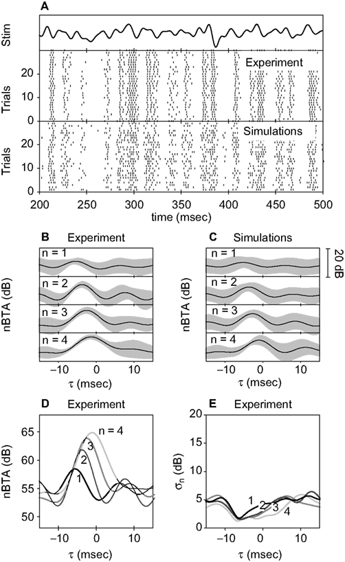
Figure 8. Definition and characteristics of the nBTA. (A) Acoustic stimulus (top) and the first 30 (out of 100) trials of the recorded (middle) and simulated (bottom) neural responses. The AM signal had a standard deviation of 6 dB and a cutoff frequency of 100 Hz. (B,C) All stimulus segments generating bursts of a given n were collected together and aligned with respect to the time of burst initiation to obtain the nBTAs, shown for real (B) and simulated (C) data. Grey areas represent the SD. (D) nBTAs as a function of time, for four different values of n. Thick lines mark the segments where each nBTA is significantly different from the other three, as assessed with a Student’s t-test (p < 0.01). (E) The standard deviation of each nBTA as a function of time (see Eq. 14). Approximately 7 msec before the first spike of a burst is recorded, the standard deviation shows a minimum, implying that at this moment the different stimuli preceding an n-burst are most similar. This time lag was similar for all n.
The standard deviation σn(τ) of all stimuli generating n bursts provides a measure of the dissimilarity between the stimulus segments. If there is a particular τ for which σn(τ) becomes markedly small, then, for that time τ, the stimuli preceding an n burst are noticeably similar to each other. In Figure 8
E, σn(τ) is depicted. There is a clear minimum ∼7 msec before burst generation, coinciding with the sharp upstroke in the nBTA. This delay includes sound propagation (≈1 msec) and axonal delays (≈2 msec). Notice that the position of this minimum remains roughly unchanged, as n is varied. Its standard deviation for different n-values is 0.33 msec, for this cell. The constancy of the location of the minima also holds at the population level. The mean standard deviation of the position of the minima of σn(τ) was roughly 0.05 times the inverse cutoff frequency. Its average among all bursting cells is 0.4 msec (SD 0.7 msec) considering 1 ≤ n ≤ 4.
For 98% of the bursting cells and for all n-values, σn(τ) was smaller than the standard deviation σ(τ) of the stimuli preceding all spikes (prior to any classification). The population average of the ratio of the minimum value of σ(τ) to the n-average of the minimum values of σ(τ) was 1.62 (SD 0.56). The set of stimuli preceding all spikes thus constitutes a more heterogeneous collection than the set of stimuli preceding an n-burst. This is not surprising. If, say, a burst of three spikes is systematically generated after one particular stimulus feature, the STA includes three time-shifted copies of the relevant feature. This threefold collection of stimuli has a larger standard deviation than the set of stimuli preceding a 3-burst. In a related study (Gollisch, 2006
), spike-time jitter was shown to broaden the STA. Our data demonstrate that burst firing, although not necessarily accompanied by jitter, gives rise to a similar effect. Therefore, whenever the tendency to fire bursts is high, the collection of stimuli preceding spike generation may show a large variance, rendering the interpretation of the STA of little use. In these cases, the burst-triggered average may provide additional insight.
Not all bursting cells display nBTAs as those shown in Figure 8
D. In some cases, for example, the central peak of the 4BTA is slightly lower than that of the 3BTA, though markedly wider. These differences reflect individual properties of different neurons. However, out of the 58 sessions where bursting cells were found, 50 exhibit nBTAs whose central peaks were significantly different from one another – except, of course, at those points where the curves cross. The remaining eight sessions corresponded to cases where bursts appeared only seldom, thereby contributing with a number of samples that was too small to assess significant differences.
A burst is a sequence of shortly interleaved spikes. Could the nBTAs obtained for high n-values shown in Figure 8
D have been obtained by combining a sequence of n interspaced 1BTAs, or even STAs? To answer this question, in Figure 9
A we compare the same 4BTA depicted in Figure 8
D with a curve obtained by combining four 1BTAs interspaced with the ISIs found in the real data. The shaded areas represent the SD of the averaged data. We see that the two curves are clearly different from each other, the real 4BTA being markedly higher and wider than the combined 1BTAs. This implies that the stimulus deflections triggering bursts of n = 4 are significantly higher than those required to generate four spikes of n = 1.
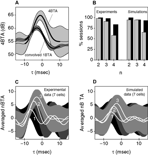
Figure 9. Analysis of the nBTAs. (A) Comparison between the 4BTA obtained for the cell depicted in Figure 8
D and the function that results from convolving four 1BTAs interspaced by the ISIs found in the real data. Thick lines denote segments that differ significantly between the two cases. Shaded areas represent the standard deviation of the averaged data. The estimated error of the 4BTA and the convolved 1BTA is ∼10 times smaller than the SD of the averaged data. (B) Black bars: Percentage of cells for which the real nBTA differs from the convolved 1BTA anywhere inside the time interval between the two minima at each side of the maximum in the nBTA, as assessed by a two-way ANOVA test. Grey bars: percentage of cells where a significant difference was found in at least 70% of the tested time interval, as assessed by a point-by-point Student’s t-test. (C) Population average of the 1BTA, 2BTA, and 3BTA for the seven cells driven with an AM signal with 100 Hz cutoff frequency and 6 dB standard deviation. Shaded areas represent the SD of the average. Black: SD of the 1BTA. Grey: SD of the 2BTA. Light grey: SD of the 3BTA. (D) Same as (C), but obtained from simulated threshold-linear cells with refractory period.
To test other cells in the population for the same effect, for each n we determined the fraction of sessions for which the nBTA differed significantly from the combined 1BTAs (or STAs) in an interval extending between the two minima at each side of the central maximum of the nBTA. This comparison was done by means of a two-way ANOVA (see Materials and Methods). Black bars depict the fraction of cells where a significant difference was found. Among the cells that exhibited significant differences, we tested whether the difference could be observed in a substantial fraction of the tested interval. To that end, we carried out a Student’s t-test for each time point within the time interval between the two minima at each side of the maximum of the nBTA (see Materials and Methods). We counted the cells showing significant differences in more than the 70% of the tested interval. The results are depicted in grey bars in Figure 9
B. A large fraction of the cells show a significant difference, for both real and simulated data. Hence, also at the population level, the nBTAs differ significantly from the convolved 1BTAs. As n increases, the number of sessions with significant differences diminishes. This is a consequence of the fact that for larger n, there are fewer n-bursts, and therefore, the error bar of the estimation of the nBTA increases. As an additional check, we repeated the analysis by convolving n shifted copies of the STA, instead of the 1BTA, obtaining similar results.
Finally, we checked that for the same stimulus, the nBTAs of different cells showed a similar trend, as n varied. The population average was taken after subtracting the mean stimulus to each nBTA because different receptors were recorded with different mean stimuli (see Materials and Methods). In addition, since different cells showed different latencies τn, all stimulus segments were shifted by τn before averaging, and then shifted back afterwards. Figure 9
C demonstrates that also at the population level, high-n bursts are associated with either higher or wider stimulus deflections (or both). The large error bars indicate that there is no absolute value of a stimulus fluctuation that uniquely triggers bursts of a given n-value, throughout the population. The qualitative behavior is also reproduced by the threshold-linear model with refractory Period (Figure 9
D). We conclude that both in real and modeled data, high-n bursts are associated with high or wide stimulus deflections.
Let us turn to the analysis of P[n|s(τ)] and describe how this quantity varies with the height of the deflections in s(τ). The shape of the nBTAs (Figure 8
D) demonstrates that the average stimulus preceding an n-burst always contained a prominent up-and-down excursion, whose maximum was located some τn milliseconds before burst initiation. This indicates that there is an association between upward stimulus excursions and burst generation. Can we assert that the probability of generating a burst of n spikes at a given time depends on the size of the upward stimulus excursion? In order to explore this question, we estimated the probabilities P(n|h) of obtaining bursts of n spikes following an upward stimulus excursion of height h (see Materials and Methods). For an example cell, Figure 10
shows a marked segregation between the responses elicited by deflections of different heights. Whereas fairly low excursions produce either no response (dotted line) or an isolated spike (black, solid line), large deflections are associated with doublets (dark grey), triplets (grey), or bursts with four spikes (light grey line). All cells showing a bursting behavior exhibited this phenomenon.
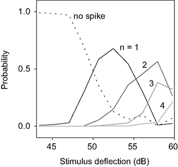
Figure 10. Probability of generating no response (dotted line), an isolated spike (black, solid line), a spike doublet (dark grey) or triplet (grey), or a burst with four spikes (light grey line) as a function of the height of the stimulus deflection, for an example cell. The uncertainties of these probabilities have been estimated (Samengo, 2002
), and the absolute error was always below 0.025. The segregation between the lines indicates that the number of spikes in a burst contains information about the height of the stimulus upward excursion preceding the burst.
The role of burst firing for neural coding has been studied extensively in systems where individual neurons have an intrinsic tendency to burst. Typical examples are electrosensory neurons of electric fish (Metzner et al., 1998
; Oswald et al., 2004
) and thalamic relay cells in the visual systems of cat (Alitto et al., 2005
; Denning and Reinagel, 2005
; Lesica et al., 2006
) and mouse (Grubb and Thompson, 2005
). For downstream neurons, however, it is irrelevant how bursts are generated. All that matters is their representational properties, i.e., their structure and coding capability. Therefore, we have focused on the coding properties of cells that lack intrinsic burst mechanisms. In particular, we wanted to know how much sensory information is transmitted and which symbols in the neural code are associated with each stimulus feature. To that end, we analyzed the activity of grasshopper auditory receptor neurons and simulated neurons, both lacking intrinsic bursting mechanisms. We first introduced a criterion that allowed us to determine the cases where a neural response could be considered as a sequence of bursts. Next, we explored a code based on the intra-burst spike count n. We estimated the information transmitted by this code, and characterized the correspondence between specific stimulus features and specific n-values. We observed that long bursts are associated with particularly high or long stimulus excursions, and that this effect could not be reproduced by concatenating the stimuli generating short bursts. In the following subsections, we discuss our results in the context of previous studies.
Burst Identification Benefits from Considering Neural Response Statistics
In previous analyses, burst identification typically relied on strict boundaries on the ISIs (see, for example, Alitto et al., 2005
; Denning and Reinagel, 2005
; Lesica and Stanley, 2004
; Oswald et al., 2004
). This is appropriate for cells that have intrinsic burst mechanisms with fairly rigid time constants. However, neurons that do not burst intrinsically exhibit intra-burst ISIs of variable duration, depending on the temporal properties of the stimulus as shown by a comparison of the peak widths in Figures 3
B,G. Hence, in this work the criterion used to determine whether two consecutive spikes were or were not part of a burst was uniquely tailored for each session. Note that if a cell is classified as non-bursting, this does not imply that it does not generate bursts at all, but rather, that the intra-burst ISIs (if present) cannot be cleanly separated from the inter-burst ISIs. In these cases it is not possible to interpret the neural code in terms of distinct words formed by closely spaced spikes.
Burst Coding does not Require Intrinsic Burst Dynamics
Not all cells investigated in this study were bursters: Some cells bursted in response to some stimuli, and responded tonically to other stimuli. Indeed, grasshopper receptors do not burst when driven with constant or step stimuli (Gollisch and Herz, 2004
; Gollisch et al., 2002
). In other studies, the time-scales of stimuli eliciting bursts have often been related to the particular ionic currents involved in burst generation (Alitto et al., 2005
; Denning and Reinagel, 2005
;Dorion et al., 2007
; Krahe and Gabbiani, 2004
; Lesica et al., 2006
). Oswald et al. (2004)
also presented a mathematical model in which bursts were only able to support efficient feature detection when a specific active dendritic backpropagation was present. Our results, however, demonstrate that burst-coding does not require complex intrinsic neural dynamics, as shown by our minimal computational model (see Keat et al., 2001
, for another example). Although simulated neurons were in general less precise than real neurons, they showed similar correlation functions (Figure 3
), and coding properties (Figures 7 and 8
). These findings underscore that the tendency to burst does not need to be an intrinsic propensity of the cell per se, but may arise as a consequence of how its cellular properties interact with the temporal characteristics of the external stimulus. Our system, therefore, is an example of stimulus-induced bursting as previously reported by Neiman et al. (2007)
.
Comparison with Other Neural Codes
We have assumed that the relevant code symbols are the time at which a burst is initiated, and the intra-burst spike count n. There are, however, other burst-based neural codes that have been explored previously. For example, Kepecs et al. (2002
, unpublished) reported that the relevant information can be encoded in the total duration of a burst. In the cells of our study, n was proportional to burst duration (data not shown). This implies that for those neurons a code based on the intra-burst spike count n is equivalent a burst-duration code. On the other hand, in electrosensory neurons of electric fish, ISIs in bursts with two spikes depend on the amplitude of electric-field upstrokes was encoded in the duration of ISIs of bursts of n = 2 (Oswald et al., 2007
). Grasshopper auditory receptors, however, have rather narrow ISI range of at most 3 msec, to be compared with the typical range of 8 msec in electric fish. We have therefore not explored a code utilizing the intra-burst ISI length.
Previous studies have also reported n-based neural codes in different sensory modalities. In visual cortex, for example, n depends on stimulus orientation, as shown by DeBusk et al. (1997)
, Martinez-Conde et al. (2002) and others. In the vertebrate retina, n carries information about the stimulus history preceding burst initiation (Berry et al., 1997
). Experimental data from cat LGN (Kepecs et al., 2001
; Kepecs et al., unpublished) and computational models (Kepecs et al., 2002
) demonstrate that n can encode the slope of stimulus upstrokes.
We would like to emphasize that an n-burst code differs from a firing-rate code. Within a firing-rate code, each point in time is associated with a specific time-dependent firing rate. This rate may be computed as an instantaneous firing rate from local ISIs, or by convolving the spike train with a certain filter function. In either case, the precise time course of the original spike train may be fully recovered. This is not true for the n-burst code, where information about the exact spike times within each burst is lost – in essence, the code only looks at whether there is a spike within the time interval defined through the correlation function, or not. Thus, the n-burst code provides a highly reduced representation, and not a full firing-rate code.
Our analysis shows, however, that in spite of this reduction the n-burst code still contains a large fraction (∼85%) of the total transmitted information, as deduced from comparing our results with the direct method. In addition, by parsing the responses into code-words, the code is amenable for read-out. Our results show significant differences between the stimuli encoded by different n-values and reveal those stimuli explicitly.
Implications for the Neural Code
We have also derived a procedure to calculate the mutual information rate between stimuli and responses if different bursts can be assumed to be independent from each other. This technique should be extended with caution to other systems since the small size of inter-burst correlations found in grasshopper auditory receptors may not be shared by other sensory systems. In addition, vanishing inter-burst correlations do not guarantee that the bursts be independent. Higher-order correlations could still be present. Our approximation assumes that those terms can be neglected when computing information measures.
The consequence of assuming that different n-bursts are independent from one another is that the total transmitted information may be decomposed into the sum of the information transmitted by each n-burst. This allows one to quantify which n-values are most relevant. Our data show that n-bursts with n > 1 can transmit at least the same amount of information as isolated spikes (n = 1).
To analyze the relation between particular n-values and the stimuli represented by these bursts, we calculated burst-triggered averages for each n. The set of stimuli preceding different n-values differed significantly from one another. Specifically, n was shown to be reliably associated to the height of the stimulus upstroke preceding burst generation. In some cells, a weak dependence on the width of the amplitude deflection, its slope, and its integral was observed, too (data not shown). However, at the population level, the stimulus feature that most reliably co-varied with n was the maximal height of the AM signal.
The two aspects that seem to be most relevant for information transmission, i.e., the time at which a burst is initiated and the intra-burst spike count n, would also be good candidates to represent what in the literature has been distinguished as the when and the what in a stimulus (Berry et al., 1997
; Borst and Theunissen, 1999
; Theunissen and Miller, 1995
). In our data, bursts containing different numbers of spikes are associated with sound fluctuations of different heights and widths. The n-value thus provides qualitative information about two key stimulus aspects. In addition, the time at which a burst begins indicates when the corresponding acoustic feature occurred. Notice that both aspects are interwoven, because the response latency decreases with increasing n. To decode the precise arrival time of an acoustic signal, downstream neurons therefore also need to read out the intra-burst spike count n. This provides additional independent evidence for the usefulness of the n burst code investigated in this study.
The authors declare that the research was conducted in the absence of any commercial or financial relationships that could be construed as a potential conflict of interest.
We are grateful to Adam Kepecs for sharing his unpublished manuscript A burst-duration code in the thalamus with us. We thank Tim Gollisch and Germán Mato for useful discussions. This work was supported by the Alexander von Humboldt Foundation, the Deutsche Forschungsgemeinschaft (SFB 618), the Consejo de Investigaciones Científicas y Técnicas, the German Federal Ministry of Education and Research, the Israeli Ministry of Science, the Minerva Foundation of the Max Planck Society, and the Secretaría de Ciencia y Tecnología of Argentina.