1
Department of Neurobiology, State University of New York Stony Brook, Stony Brook, NY, USA
2
Kalypso Institute, Stony Brook, NY, USA
Learning is thought to occur by localized, activity-induced changes in the strength of synaptic connections between neurons. Recent work has shown that induction of change at one connection can affect changes at others (“crosstalk”). We studied the role of such crosstalk in nonlinear Hebbian learning using a neural network implementation of independent components analysis. We find that there is a sudden qualitative change in the performance of the network at a threshold crosstalk level, and discuss the implications of this for nonlinear learning from higher-order correlations in the neocortex.
Unsupervised artificial neural networks usually use local, activity-dependent (and often Hebbian) learning rules, to arrive at efficient, and useful, encodings of inputs in a self-organizing manner (Herz et al., 1991
; Haykin, 1994
). It is widely believed that the brain, and particularly the neocortex, might self-organize, and efficiently represent an animal’s world, in a similar way (Dayan and Abbott, 2001
; Cooper et al., 2004
), especially since synapses exhibit spike-coincidence-based Hebbian plasticity (Andersen et al., 1977
; Levy and Steward, 1979
; Dan and Poo, 2004
), such as long-term potentiation (LTP) or long-term depression (LTD). However, some data (Kossel et al., 1990
; Bonhoeffer et al., 1994
; Schuman and Madison, 1994
; Engert and Bonhoeffer, 1997
; Bi, 2002
) suggest that biological Hebbian learning may not be completely synapse-specific, and other data (Chevaleyre and Castillo, 2004
; Matsuzaki et al., 2004
), while showing a high degree of specificity, do not unequivocally show complete specificity. Very recent work (Harvey and Svoboda, 2007
) has shown that induction of LTP at one synapse modifies the inducibility of LTP at closely neighboring synapses (“crosstalk”). Perhaps, given the close packing of synapses in neuropil (>109 mm−3 in neocortex; DeFelipe et al., 1999
), complete chemical isolation may be impossible. Such crosstalk, although typically very small, could nevertheless lead to inaccurate adjustments of connection strengths during development or learning. Our work focuses on the idea that extremely accurate connection strength adjustments might be required for the type of learning that occurs in the neocortex, and that if the necessary extreme accuracy is biophysically impossible, some characteristic, and enigmatic, neocortical circuitry might boost accuracy and allow useful learning (Cox and Adams, 2000
; Adams and Cox, 2002a
,b
, 2006
).
In previous work we studied the effect of learning inaccuracy, or crosstalk, in simplified neural network models using a linear Hebbian learning rule, which is only sensitive to pairwise correlations (Cox and Adams, 2000
; Adams and Cox, 2002a
,b
; Radulescu et al., 2009
). We found that useful learning is always still possible provided that Hebbian adjustments retain some connection specificity, though it is degraded. However, there has been increasing realization that at least in the neocortex unsupervised learning must be sensitive to higher-than-pairwise correlations, which requires that the learning rule at individual connections be nonlinear. Since the number of possible higher-order correlations is, for high-dimensional input patterns, essentially unlimited, useful learning might require that the connection-level nonlinear learning rule be extremely accurate.
To test this idea, we studied the effect of introducing Hebbian crosstalk in perhaps the simplest neural network model of nonlinear learning, independent components analysis (ICA) (Nadal and Parga, 1994
; Bell and Sejnowski, 1995
; Hoyer and Hyvärinen, 2000
; Hyvärinen et al., 2001
). In this model, it is assumed that the higher-order correlations between inputs arise because these vectors are generated from independent, non-Gaussian sources by a linear mixing process. The goal of the nonlinear learning process is to estimate synaptic weights corresponding to the inverse of the mixing matrix, so that the network can recover the unknown sources from the given input vectors (Nadal and Parga, 1994
; Bell and Sejnowski, 1995
; Hyvärinen et al., 2001
). We are not proposing that the brain actually does ICA, although the independent components of natural scenes do resemble the receptive fields of neurons in visual cortex (Bell and Sejnowski, 1997
; van Hateren and Ruderman, 1998
; van Hateren and van der Schaaf, 1998
; Hyvärinen and Hoyer, 2000
). Furthermore, ICA is closely related to projection pursuit and the Bienenstock–Cooper–Monro rule, which have been proposed as important for neocortical plasticity (Cooper et al., 2004
). ICA is a special, particularly tractable case (linear square noiseless mixing) of the general unsupervised learning problem. While our approach incorporates one aspect of biological realism (i.e. imperfect specificity), we make no attempt to incorporate others (e.g. spike-timing dependent plasticity, overcomplete representations, observational noise, nonlinear mixing, temporal correlations, synaptic homeostasis etc.), since these are being studied by others. The goal of this work is to investigate crosstalk in the simplest possible context, rather than to propose a detailed model of biological learning. Although our model is extremely oversimplified, there is no reason to suppose that more complicated models would be more crosstalk-resistant, unless they were specifically designed to be so.
Our computer experiments, described below, suggest that slight Hebbian inspecificity, or crosstalk, can make learning intractable even in simple ICA networks. If crosstalk can prevent learning even in favorable cases, it may pose a general, but hitherto neglected, barrier to unsupervised learning in the brain. For example, since crosstalk will increase with synapse density, our results suggest an upper bound on the number of learnable inputs to a single neuron. We propose that some of the enigmatic circuitry of the neocortex functions to raise this limit, by a “Hebbian proofreading” mechanism.
We were unable to extend Amari’s analysis (Amari et al., 1997
) of the stability of the error-free learning rule to the erroneous case, so we relied on numerical simulation, using Matlab. Except for Figure 5
, all simulations stored data only for every hundredth iteration, or epoch. Most of our results were obtained using the Bell–Sejnowski (Bell and Sejnowski, 1995
) multi-output rule, but in the last section of Results we used the Hyvarinen–Oja single output rule (Hyvarinen and Oja, 1998
).
An n-dimensional vector of independently fluctuating sources s obtained from a defined (usually Laplacian) distribution was mixed using a mixing matrix M (generated using Matlab’s “rand” function to give an n by n-dimensional matrix with elements ranging from {0,1} and sometimes {−1,1}), to generate an n-dimensional column vector x=M s, the elements of which are linear combinations of the sources, the elements of s. For a given run M was held fixed, and the numeric labels of the generating seeds, and sometimes the specific form of M, are given in the Results or Appendix (since the result depended idiosyncratically on the precise M used). However, in all cases many different Ms were tested, creating different sets of higher-order correlations, so our conclusions seem fairly general (at least within the context of the linear mixing model).
The aim is to estimate the sources s1, s2,…,sn from the mixes x1, x2,…,xn by applying a linear transformation W, represented neurally as the weight matrix between a set of n mix neurons whose activities constitute x and a set of n output neurons, whose activities u represents estimates of the sources. When W=PM−1 the (arbitrarily scaled) sources are recovered exactly (P is a permutation/scaling matrix which reflects uncertainties in the order and size of the estimated sources). Although neither M nor s may be known in advance, it is still possible to obtain an estimate of the unmixing matrix, M−1, if the (independent) sources are non-Gaussian, by maximizing the entropy (or, equivalently, non-Gaussianity) of the outputs. Maximizing the entropy of the outputs is equivalent to making them as independent as possible. Bell and Sejnowski (1995)
showed that the following nonlinear Hebbian learning rule could be used to do stochastic gradient ascent in the output entropy, yielding an estimate of M−1,

where u (the vector of activities of output neurons)=Wx and y=f(u)=g″(u)/g′(u) where g(s) is the source cdf, primes denote derivatives and γ is the learning rate.
Amari et al. (1997)
showed that even if f ≠ g″/g′, the algorithm still converges (in the small learning rate limit) to M−1 if certain conditions on f and g are respected.
Bell and Sejnowski derived specific forms of the Hebbian part of the update rule assuming various nonlinearities (matching different source distributions). For the logistic function  their rule, which we will call the BS rule, is (for superGaussian sources):
their rule, which we will call the BS rule, is (for superGaussian sources):
where 1 is a vector of ones. Using Laplacian sources the convergence conditions are respected even though the logistic function does not “match” the Laplacian. The first term is an antiredundancy term which forces each output neuron to mimic a different source; the second term is antiHebbian (in the superGaussian case), and could be biologically implemented by spike coincidence-detection at synapses comprising the connection It should be noted that the matrix inversion step is merely a formal way of ensuring that different outputs evolve to represent different sources, and is not key to learning the inverse of M. We also tested the “natural gradient” version of the learning rule (Amari, 1998
), where the matrix inversion step is replaced by simple weight growth (multiplication of Eq. 1 by WTW), which yielded faster learning but still gave oscillations at a threshold error. We also found that a one-unit form of ICA (Hyvarinen and Oja, 1998
), which replaces the matrix inversion step by a more plausible normalization step, is also destabilized by error (Figure 8
). Thus although the antiredundancy part of the learning rule we study here may be unbiological, the effects we describe seem to be due to the more biological Hebbian/antiHebbian part of the rule, which is where the error acts.
Errors were implemented by postmultiplying the Hebbian part of ΔW by an error matrix E (components Eij; see below), which shifted a fraction Eij of the calculated Hebbian update (1 − 2y)xT from the jth connection on an output neuron onto the ith connection on that neuron, i.e. postsynaptic error (Figure 1
, left).
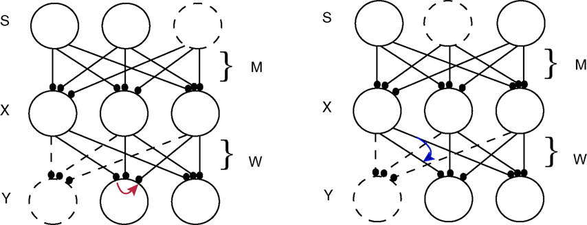
Figure 1. Schematic ICA network. Mixture neurons X receive weighted signals from independent sources S, and output neurons Y receive input from the mixture neurons. The goal is for each output neuron to mimic the activity of one of the sources, by learning a weight matrix W that is the inverse of M. In the diagrams this is indicated by the source shown as a dotted circle being mimicked by one of the output neurons (dotted circle) with the dotted line connections representing a weight vector which lies parallel to a row of M−1, i.e. an independent component or “IC” . The effect of synaptic update error is represented by curved colored arrows, red being the postsynaptic case (crosstalk between synapses on the same postsynaptic neuron, left diagram), and blue the presynaptic case (crosstalk between synapses made by the same presynaptic neuron; right diagram). In the former case part of the update appropriate to the connection from the left X cell to the middle Y cell leaks to the connection from the right X cell to the middle Y cell, e.g. by. In the latter case, part of the update computed at the connection from the left X cell onto the right Y cell leaks onto the connection from the left X cell onto the middle Y cell. However, in both these cases for clarity only one of the n2 possible leakage paths that comprise the error matrix E (see text) are shown. Note that learning of W is driven by the activities of X cells (the vector x) and by the nonlinearly transformed activities of the Y cells (the vector y), as well as by an “antiredundancy” process.

This reflects the assumption that Hebbian changes are induced and expressed postsynaptically. Premultiplying by E would assign error from the ith connection on a given output neuron onto the jth connection on another output neuron made by the same presynaptic neuron (presynaptic error; Figure 1
, right). We will analyze this presynaptic case elsewhere.
The Error Matrix
The errors are implemented (“error onto all”, see below) using an error matrix E:
where Q is the fraction of update that goes on the correct connection and ε=(1 − Q)/(n − 1) is the fraction that goes on a wrong connection. The likely physical basis of this “equal error-onto-all” matrix is explained below (see also Radulescu et al., 2009
). We often refer to a “total error” E which is 1 − Q. When ε=Q, specificity breaks down completely, and, trivially, no learning at all can occur.
Error onto All
The proposed physical basis of the lack of Hebbian specificity studied in this paper is intersynapse diffusion, for example of intracellular calcium. In principle intersynapse diffusion will only be significant for synapses that happen to be located close together, and it seems likely, at least in neocortex (e.g. Markram et al., 1997
), that the detailed arrangements of synapses in space and along the dendritic tree will be arbitrary (reflecting the happenstance of particular axon-dendrite close approaches) and unrelated to the statistical properties of the input. This would reflect the standard connectionist view that synaptic potentials occurring anywhere on the dendrites are “integrated” at the initial segment, and might not hold if important computations are done in nonlinear dendritic domains (Hausser and Mel, 2003
). Nevertheless, in the present work we made the simplest possible assumption, that all connection strength changes are equally likely to affect any other connection strength – an idea we call “equal error onto all”. The underlying premise is that there should be no arbitrarily privileged connections – that the neural learning device should function as a “tabula rasa” (Kalisma et al., 2005
; Le Be and Markram, 2006
) – which is inherent in the connectionist approach. We extend the idea that all connections should be approximately electrically equivalent (Nevian et al., 2007
) to suggest that they might also be approximately chemically equivalent. This could also be viewed as a “meanfield” assumption, so that “anatomical fluctuations” (detailed synaptic neighborhood relations) get averaged out in the large n limit, because messengers spread (Noguchi et al., 2005
; Harvey et al., 2008
), connections turn-over (Stepanyants et al., 2002
; Chklovskii et al., 2004
; Kalisma et al., 2005
; Keck et al., 2008
) and are multisynapse (Binzegger et al., 2004
), as discussed in (Radulescu et al., 2009
). In the limit of the error-onto-all assumption, the diagonal elements, and also the off-diagonal elements, of E are equal, and in the case of complete specificity E reduces to the identity matrix implicit in conventional treatments of Hebbian learning. However, in reality the exact distribution of errors, even for multisynapse labile connections, will vary according to the idiosyncratic arrangement of particular axon-dendrite touchpoints. We also tested examples of E where offdiagonal elements were perturbed randomly away from equality, with very similar qualitative results. Of course, if synapses carrying strongly correlated signals cluster on dendrites, local crosstalk might actually be useful (Hausser and Mel, 2003
). However, we do not know of evidence that such clustering occurs in the neocortex (see Discussion).
The “quality” Q of the learning process (Q=1 is complete specificity), would depend on the number of inputs n, the dendritic (e.g. calcium) diffusion length constant, the spine neck and dendritic lengths, and buffering and pumping parameters. In the simplest case, with a fixed dendritic length, as n increases the synapse linear density increases proportionately, and one expects Q=1/(1 + nb) where b is a “per synapse” error rate. This expression can be derived as follows (see also Discussion and Radulescu et al., 2009
). Call the number of existing (silent or not) synapses comprising a connection α. The total number of synapses on the dendrite, N, is therefore N=nα and the synapse density ρ is nα/L where L is the dendrite length. Define x as the linear dendritic distance between the shaft origins of two spiny synapses. For x=0, assume that the effective calcium concentration in an unstimulated synapse is an “attenuation” fraction a of that in the head of a synapse undergoing LTP, due to outward calcium pumping along two spine necks in series. Assume that calcium decays exponentially with distance along the shaft (Zador and Koch, 1994
; Noguchi et al., 2005
) with space constant λc, and that the LTP-induced strength change at a synapse is proportional to calcium. The expected total strengthening at neighboring synapses due to calcium spread from a reference synapse at x=0 where LTP is induced, as a fraction of that at the reference synapse, assuming that λc is much smaller than half the dendritic length, is given by:
where 
b (a “per connection error rate”) reflects intrinsic physical factors that promote crosstalk (spine–spine attenuation and the product of the per-connection synapse linear density and λc), while n reflects the effect of adding more inputs, which increases synapse “crowding” if the dendrites are not lengthened (which would compromise electrical signaling; Koch, 2004
). Notice that silent synapses would not provide a “free lunch” – they would increase the error rate, even though they do not contribute to firing. Although incipient (Adams and Cox, 2002a
,b
) or potential (Stepanyants et al., 2002
) synapses would not worsen error, the long-term virtual connectivity they provide could not be immediately exploited. We ignore the possibility that this extra, unwanted, strengthening, due to diffusion of calcium or other factors, will also slightly and correctly strengthen the connection of which the reference synapse is part (i.e. we assume n is quite large). This treatment, combined with the assumption that all connections are anatomically equivalent (by spatiotemporal averaging), leads to an error matrix with 1 along the diagonal and nb/(n − 1) offdiagonally. In order to convert this to a stochastic matrix (rows and columns sum to one, as in E defined above) we multiply by the factor 1/(1 + nb), giving Q=1/(1 + nb). We ignore the scaling factor (1 + nb) that would be associated with E, since it affects all connections equally, and can be incorporated into the learning rate. It’s important to note that while b is typically biologically very small (∼10−4; see Discussion), n is typically very large (e.g. 1000 in the cortex), which is why despite the very good chemical compartmentation provided by spine necks (small a), some crosstalk is inevitable.
The off diagonal elements Ei, j are given by (1 − Q)/(n − 1). In the results we use b as the error parameter but specify in the text and figure legends where appropriate the “total error” E=1 − Q, and a trivial error rate εt=(n − 1)/n when specificity is absent.
Orthogonal Mixing Matrices
In Sections Orthogonal Mixing Matrices and Hyvarinen–Oja One-Unit Rule, an orthogonal, or approximately orthogonal, mixing matrix MO was used. A random mixing matrix M was orthogonalized using an estimate of the inverse of the covariance matrix C of a sample of the source vectors that had been mixed using M. M was then premultiplied by the decorrelating matrix Z computed as follows:
 and Mo=Z M
The input vectors x generated using MO constructed in this way were thus variably “whitened”, to an extent that could be set by varying the size of the sample (the batch size) used to estimate C. The performance of the network was measured against a new solution matrix  which is approximately orthogonal, and is the inverse of the original mixing matrix M premultiplied by Z, the decorrelating, or whitening, matrix:
which is approximately orthogonal, and is the inverse of the original mixing matrix M premultiplied by Z, the decorrelating, or whitening, matrix:
In another approach, perturbations from orthogonality were introduced by adding a scaled matrix (R) of numbers (drawn randomly from a Gaussian distribution) to the whitening matrix Z. The scaling factor (which we call “perturbation”) was used as a variable for making MO less orthogonal, as in Figure 6
(see also Appendix Methods).
One-Unit Rule
For the one-unit rule (Hyvarinen and Oja, 1998
) we used Δw=−γ x tanh(u) followed by division of w by its Euclidian norm. The input vectors were generated by mixing source vectors s using a whitened mixing matrix MO (described above, and see Appendix). For the simulations the learning rate γ was 0.002 and the batch size for estimating the covariance matrix was 1000. At each error value the angle between the first row of  , and the weight vector was allowed to reach a steady value and then the mean and standard deviation was calculated from a further 100,000 epochs.
, and the weight vector was allowed to reach a steady value and then the mean and standard deviation was calculated from a further 100,000 epochs.Bs Rule With Two Neurons and Random M
We first looked at the BS rule for n=2, with a random mixing matrix. Figure 2
shows the dynamics of initial, error-free convergence for each of the two weight vectors, together with the behaviour of the system when error is applied. “Convergence” was interpreted as the maintained approach to 1 of one of the cosines of the angles between the particular weight vector and each of the possible rows of M−1 (of course with a fixed learning rate exact convergence is impossible; in Figure 2
, γ=0.01, which provided excellent initial convergence). Small amounts of error, (b=0.005, equivalent to total error E=0.0099, applied at 200,000 epochs) only degraded the performance slightly. However, at a threshold error rate (bt=0.01037, E=0.0203 see Figure 4
A and Appendix) each weight vector began, after variable delays, to undergo rapid but widely spaced aperiodic shifts, which became more frequent, smoother and more periodic at an error rate of 0.02 (E=0.0384; Figure 2
). These became more rapid at b=0.05 (see Figure 4
A) and even more so at b=0.1 (Figure 2
, E=0.166). Figure 2
D shows that the individual weights on one of the output neurons smoothly adjust from their correct values when a small amount of error is applied, and then start to oscillate almost sinusoidally when error is increased further. Note that at the maximal recovery from the spike-like oscillations the weight vector does briefly lie parallel to one of the rows of M−1.
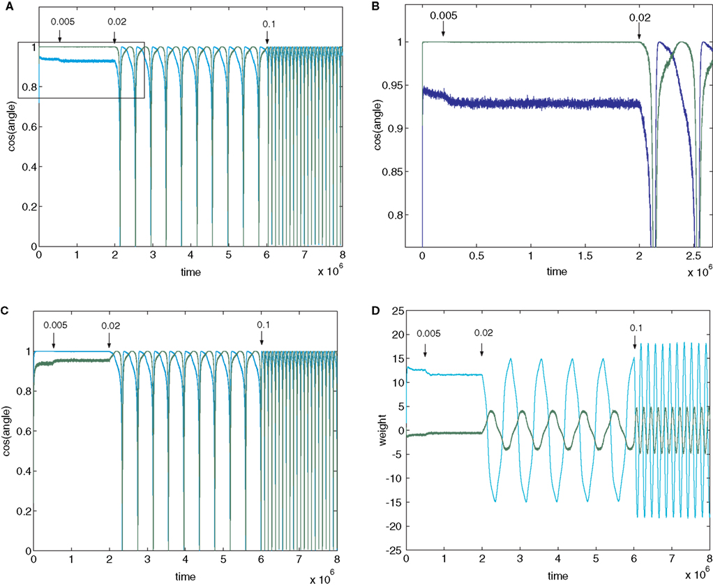
Figure 2. Plots (A) and (C) shows the initial convergence and subsequent behaviour, for the first and second rows of the weight matrix W, of a BS network with two input and two output neurons Error of b=0. 005 (E=0.0099) was applied at 200,000 epochs, b=0.02 (E=0.0384) at 2,000,000 epochs. At 6,000,000 epochs error of 0.1 (E=0.166) was applied. The learning rate was 0.01. (A) First row of W compared against both rows of M−1 with the y-axis the cos(angle) between the vectors. In this case row 1 of W converged onto the second IC, i.e. the second row of M−1 (green line), while remaining at an angle to the other row (blue line). The weight vector stays very close to the IC even after error of 0.005 is applied, but after error of 0.02 is applied at 2,000,000 epochs the weight vector oscillates. (B) A blow-up of the box in (A) showing the very fast initial convergence (vertical line at 0 time) to the IC (green line), the very small degradation produced at b=0.005 (more clearly seen in the behavior of the blue line) and the cycling of the weight vector to each of the ICs that appeared at b=0.02. It also shows more clearly that after the first spike the assignments of the weight vector to the two possible ICs interchanges. (C) Shows the second row of W converging on the first row of M−1, the first IC, and then showing similar behaviour. The frequency of oscillation increases as the error is further increased (0.1 at 6,000,000 epochs). (D) Plots the weights of the first row of W during the same simulation. At b=0.005 the weights move away from their “correct” values, and at b=0.02 almost sinusoidal oscillations appear.
One could therefore describe the behavior as switching between assignments, though spending most of its time at nonparallel states. Similar behavior was seen with different initializations of W or s.
Orbits
Figure 3
shows plots of the components of both weight vectors (i.e. the two rows of the weight matrix, shown in red or blue) against each other as they vary over time. The weight trajectories are shown as error is increased from 0 to a subthreshold value and then to increasingly suprathreshold values. The weights first move rapidly from their initial random values to a tight region of weight space (see blow-up in right plot), which corresponds to a choice of almost correct ICs, where they hover for the first million epochs. The initial IC found is typically the one corresponding to the longest row of M−1, and the weight vector that moves to this IC is the one that is initially closest to it (a repeat simulation is shown in Appendix Results; the initial weights were different and so was the choice). Introduction of subthreshold error produces a slight shift to an adjacent stable region of weight space. Introduction of suprathreshold error initiates a limit cycle-like orbit. Further increases in error generate longer orbits. The red and blue orbits superimpose, presumably because the two weight vectors are now equivalent, but the columns of W are phase-shifted (see orbits, Figure A4
, shown in Appendix Results). In Figure 3
the weights spend roughly equal amounts of time everywhere along the orbits, but at error rates just exceeding the threshold the weights tarry mostly very close to the stable regions seen at just subthreshold error (i.e. the weights “jump” between degraded ICs; see Appendix Results, Figures A1
–A3
).
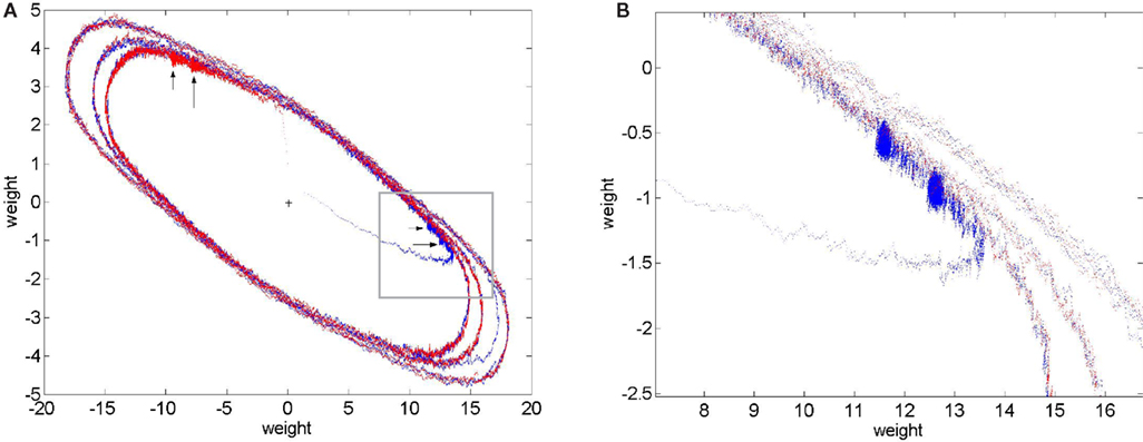
Figure 3. Trajectories of weights comprising the ICs. The weights comprising each IC (rows of the weight matrix) were plotted against each other over time ((A) red plot is the first row of W and the blue plot is the second row of W). The simulation was run for 1 M epochs with no error applied and each row of W can be seen to evolve to an IC (red and blue “blobs” indicated by large arrows in panel (A)). From 2 M to 4 M epochs error b=0.005, i.e. below the threshold error level, was applied and each row of W readjusts itself to a new stable point, red and blue “blobs” indicated by the smaller arrows. From 4 M to 6 M epochs error of 0.02 was applied and each row of W now departs from a stable point and moves off onto a limit cycle-like trajectory (inner blue and red ellipses). Error is increased at 6 M epochs to 0.05 and the trajectories are pushed out into longer ellipses. At 7 M epochs error was increased again to 0.1 and the ellipses stretch out even more. Notice the transition from the middle ellipse to the outer one (error from 0.02 to 0.1) can be seen in the blue line (row 2 of W) in the bottom left of the plot. (B) A blow-up of the inset in (A) clearly showing the stable fixed point of row 2 of W (i.e. an IC) at 0 error (right hand blue “blob”). The blob moves a small amount to the left and upwards when error of 0.005 is applied indicating that a new stable fixed point has been reached. Further increases in error launch the weights into orbit, γ=0.005.
Varying Parameters
Figure 4
A summarizes results for a greater range of error values using the same mixing matrix M. At very low error rates the weights remain stable, but at a threshold error rate near 0.01 there is a sudden break in the graph and the oscillations abruptly appear (although initially at very low frequency). Further study showed the threshold error to be very close to 0.01037 (see Figure 4
A). The change in behaviour at the threshold error rate resembles a bifurcation from a stable fixed point, which represents a degraded version of the correct IC, to a limit cycle. However, the oscillations that appear at the threshold error value are extremely slow and aperiodic (see below and Appendix).
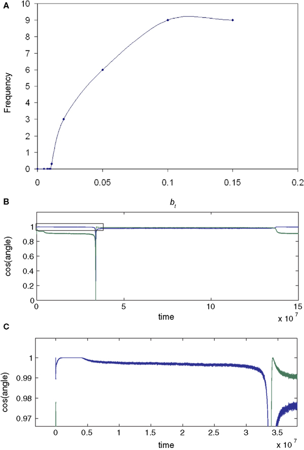
Figure 4. (A) Increased error increases the frequency of the oscillations (cycles/106 epochs) but that the onset of oscillations is sudden at b=0. 01037 (E=0.0203; L=0.01; seed=8), indicating that this threshold error level heralds a new dynamical behaviour of the network. In (B) and (C) (enlargement of the box in (B)) the behaviour of the network at a very low learning rate is shown for a different learning rate and M (γ=0.0005; seed=10). The blue curves show cos(angle) with respect to the first row of M−1, the green curves with respect to the second column. Only the results for one of the output neurons is shown (the other neuron responded in mirror-image fashion). Plot (B) shows that the weight vector converged rapidly and precisely, in the absence of error, to the first row (blue curve; the initial convergence is better seen in (C)); error (b=0.0088 E=0.0173) was introduced after five million epochs; this led to a slow decline in performance over the next five million epochs to an almost stable level which was followed by a further very slow decline over the next 30 million epochs (blue trace in (C)) which then initiated a further rapid decline in performance to 0 (the downspike in (B)) which was very rapidly followed by a dramatic recovery to the level previously reached by the green assignment; meanwhile the green curve shows that the weight vector initially came to lie at an angle about cos−1 0.95 away from the second row of M−1. The introduction of error caused it to move further away from this column (to an almost stable value about cos−1 0.90), but then to suddenly collapse to 0 at almost the same time as the blue spike. Both curves collapse down to almost 0 cosine, at times separated by about 10,000 epochs (not shown); at this time the weights themselves approach 0 (see Figure A1). The green curve very rapidly but transiently recovers to the level [cos(θ) ∼1] initially reached by the blue curve, but then sinks back down to a level just below that reached by the blue curve during the 5 M–30 M epoch period. Thus the assignments (blue to the first row initially, then green) rapidly change places during the spike by the weight vector going almost exactly orthogonal to both rows, a feat achieved because the weights shrink briefly almost to 0 (see Figure A1). During the long period preceding the return swap, one of the weights hovers near 0. After the first swapping (at 35 M epochs) the assignments remain almost stable for 120 M epochs, and then suddenly swap back again (at 140 M epochs). This time the swap does not drive the shown weights to 0 or orthogonal to both rows (Figure A1). However, simultaneous with this swap of the assignments of the first weight vector, the second weight vector undergoes its first spike to briefly attain quasi-orthogonality to both nonparallel rows, by weight vanishing (not shown). Conversely, during the spike shown here, the weight vector of the second neuron swapped its assignment in a nonspiking manner (not shown). Thus the introduction of a just suprathreshold amount of error causes the onset of rapid swapping, although during almost all the time the performance (i.e. learning of a permutation of M−1) is very close to that stably achieved at a just subthreshold error rate (b=0.00875; see Figure A1).
Different mixing matrices gave qualitatively similar results but the exact threshold error value varied (see below). The results in Figures 2
, 3 and 4
A were obtained with γ = 0.01. Lowering the learning rate produces very minor, and probably insignificant, changes in the estimated threshold error rate. Figure 4
B shows the behavior at much lower learning rates (0.0005) for a different M (seed 10), over a long simulation period (150 M epochs). The introduction of b=0.0088 (E=0.0173) at 4 M epochs lead to a slow drop in the cosine which then crept down further until the sudden onset of a very slow oscillation at 35 M epochs; the next oscillation occurred at 140 M epochs. With b=0.00875 (E=0.0172) learning was perfectly stable over 68 M epochs, though degraded (data not shown). In this case the threshold appears to lie between 0.00875 and 0.0088, though possibly there are extremely slow oscillations even at 0.00875.
If γ was increased to 0.005 there was no clear change in the threshold error rate. There was no oscillation within 60 M epochs at 0.0086 error (using seed 10) but an oscillation appeared (after 4 M epochs) at 0.0875 (see below). However the “oscillations” close to the threshold error are quite irregular: at b=0.0088 (γ=0.005) the oscillation frequency was 4.18 ± 0.31 mean ± SD; range 4.41–3.64; n=5); at 0.087 they were even slower (around 30 M epochs) and more variable, and the weights changed in a steplike manner (see Appendix Results, Figures A1
–A3
).
To explore the range of the threshold error rate, 20 consecutive seeds (50–70) for M, i.e. 20 different random Ms (with elements from {−1,1}), were used in simulations. One of the Ms did not yield oscillations at any error although two of the weights started to diverge without limit. The average threshold per-connection error b for the remaining 19 Ms was 0.134, the standard deviation 0.16, the range 0.00875–0.475. In all these cases the threshold error was less than the trivial value.
Larger Networks
Figure 5
shows a simulation of a network with n=5. The behaviour with error is now more complicated. The dynamics of the convergence of one of the weight vectors to one of the rows of the correct unmixing matrix M−1 (i.e. to one of the five ICs) is shown (Figure 5
A; for details of M, see Appendix Results). Figure 5
A plots cos(θ) for one of the five rows of W against one of the rows of M−1. An error of b=0.05 (E=0.09) was applied at 200,000 epochs, well after initial error-free convergence. The weight vector showed an apparently random movement thereafter, i.e. for eight million epochs. Figure 5
B shows the weight vector compared to the other rows of M−1 showing that no other IC was reached. Weight vector 2 (row 2 of W) shows different behaviour after error is applied (Figure 5
C). In this case the vector undergoes fairly regular oscillations, similar to the n = 2 case. The oscillations persist for many epochs and then the vector (see pale blue line in Figure 5
D) converged approximately onto another IC (in this case row 3 of M−1) and this arrangement was stable for several thousand epochs until oscillations appeared again, followed by another period of approximate convergence after 8.5 million epochs.
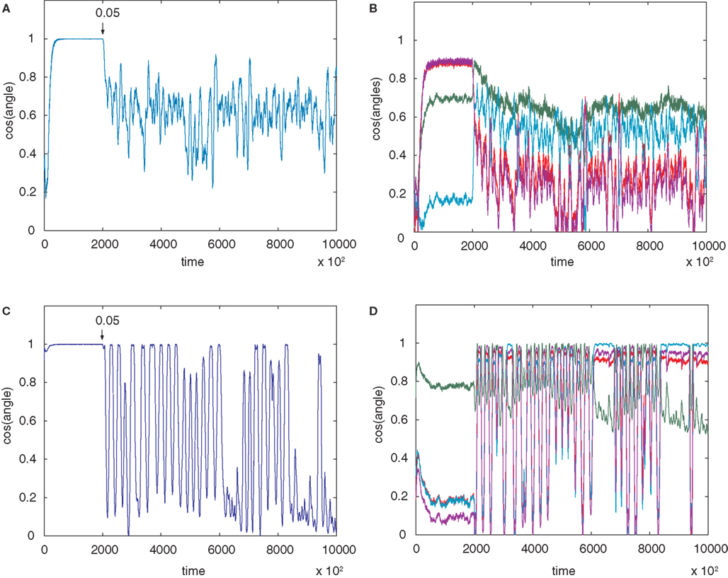
Figure 5. (A) The convergence of one of the rows of M−1, with one of the weight vectors of M (seed 8) with n=5. The initial weights of W are random. The angle between row 1 of the weight matrix and row 1 of the unmixing matrix are shown. The plot goes to 1 (i.e. parallel vectors) indicating that an IC has been reached. Without error this weight vector is stable. At 200,000 epochs error of 0.05 (E=0.09) is introduced and the weight vector then wanders in an apparently random manner. (B) The weight vector compared to all the other potential ICs and clearly no IC is being reached. Plots (C,D) on the other hand shows different behaviour for row 2 of the weight matrix (which initially converged to row 4 of M−1). In this case the behaviour is oscillatory after error (0.05 at 200,000 epochs) is introduced, although another IC (in this case row 3 of M−1 (pale blue line) after 6.5 M and again at 8.5 M epochs) is sometimes reached, as can be seen in (D) where the weight vector is plotted against all row of M−1. The learning rate was 0.01.
Orthogonal Mixing Matrices
The ICA learning rules work better if the effective mixing matrix is orthogonal, so the mix vectors are pairwise uncorrelated (whitened) (Hyvärinen et al., 2001
). For n = 2 we looked at the case where the data were whitened to varying extents. This was done either by limiting the number of data vectors used to estimate C, or by variably perturbing the whitening matrix Z (see Materials and Methods). We looked at the relationship between degree of perturbation from orthogonality of the whitened mixing matrix Q=ZC and the onset of oscillation with error (see Materials and Methods). We found that there was a correlation (Figure 6
, left graph) with the onset of oscillation occurring at lower error rates as Q was more and more perturbed from orthogonality. Figure 6
(right graph) shows the effect of lowering the batch number used in estimating the covariance matrix C of the set of source vectors that have been mixed by a random matrix M. As the effective mixing matrix, which is orthogonal with perfect whitening, becomes less orthogonal (due to a cruder estimate of the decorrelating matrix by using a smaller batch number for the estimate of C) the onset of oscillations occur at lower and lower values of error.
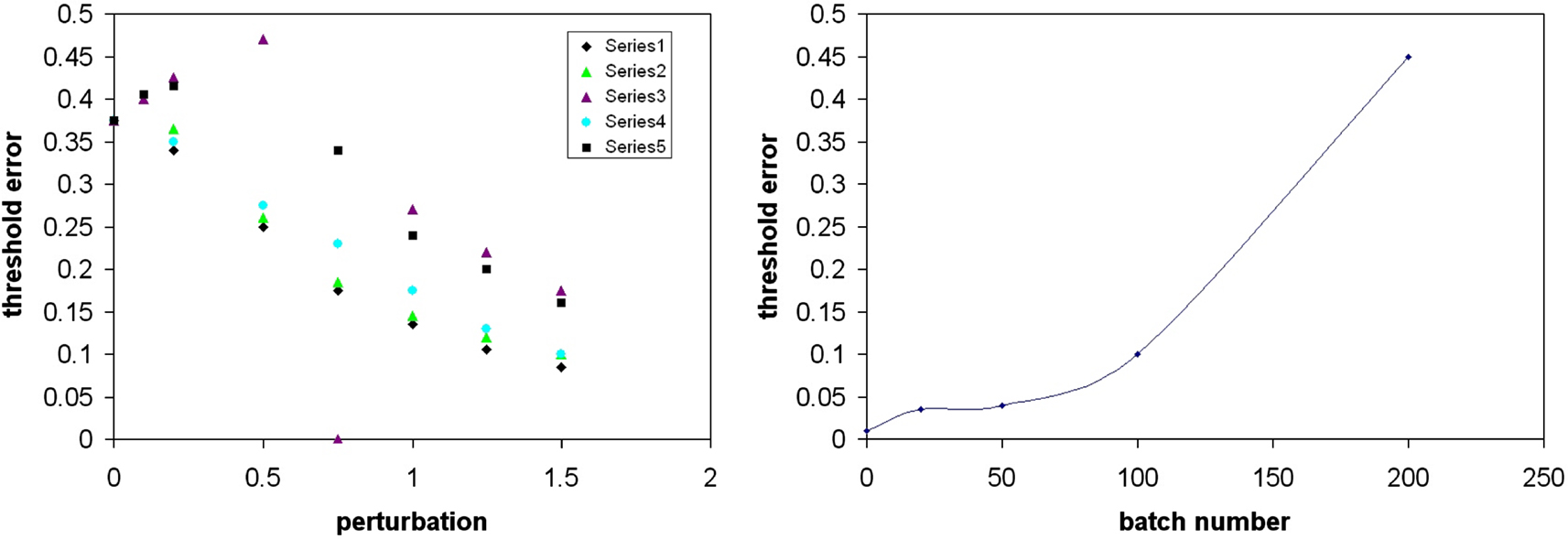
Figure 6. Effect of variable whitening on the error threshold for the onset of instability (n=5). Left figure shows the relationship between degree of perturbation of an orthogonal (whitened) matrix Q (seed 2, n=2) and the onset of oscillation. Data using five different perturbation matrices (series 1–5) applied to a decorrelating matrix Z (see Materials and Methods), are plotted. Each series is of one perturbation matrix, scaled by varying amounts (shown on the abscissa as “perturbation”), which is then added to Z (calculated from a sample of mixture vectors), and plotted against the threshold error (obtained from running different simulations using each variably perturbed Z), shown on the ordinate. At 0 perturbation (i.e. for an orthogonal effective mixing matrix) the network became unstable at a non-trivial error rate. As the effective mixing matrix was made less and less orthogonal by perturbing each of the elements of the decorrelating matrix Z (see Materials and Methods, and Appendix) the sensitivity to error increased. The right hand graph is a plot for one random M (n=5, seed 8) where the mixed data has been whitened by a decorrelating matrix,  . In this case the covariance matrix C of the mix vectors was estimated by using different batch numbers, with a smaller batch number giving a cruder estimate of C and a less orthogonal effective mixing matrix. The learning rate was 0.01 in both graphs.
. In this case the covariance matrix C of the mix vectors was estimated by using different batch numbers, with a smaller batch number giving a cruder estimate of C and a less orthogonal effective mixing matrix. The learning rate was 0.01 in both graphs.We noted above that the threshold error rate for oscillation onset varies unpredictably for different Ms. There seemed to be no relationship between the angle between the columns of M and bt (not shown). In order to try to find a relationship between a property of a given random mixing matrix and the onset of oscillation, we plotted the ratio of the eigenvalues λ2 and λ1 of MMT against bt. If M is an orthogonal matrix then MMT is the identity and λ2/λ1 is 1. If M is not orthogonal then the ratio is less than 1. We used the ratio λ2/λ1 as a measure of how orthogonal M was, and Figure 7
(left graph) shows a plot of this ratio against bt for the respective M. Although the points are scattered, there does appear to be a trend: as the ratio gets closer to 1, the value for bt gets larger. Figure 7
(right graph) is a plot of the cosine of the angle between the now normalized columns of the mixing matrices in Figure 7
(left graph) against the redetermined bt in runs for the normalized version of M. There is a clear trend indicating that the more orthogonal the normalized columns of M are, the less sensitive to error learning becomes. A few of these “normalized” matrices, however, did not show oscillation at any value of error, perhaps because the weights seemed to be growing without bound (there is no explicit normalization in the BS rule). The angles between the columns in these cases were always quite large. Completely orthogonal matrices were not, however, immune from sudden instability (i.e. at a threshold error value bt), as the two points lying on the x-axis in Figure 7
(right graph) demonstrate; here the angle between the columns is 90° but there was a threshold error rate at b=0.4 and 0.45, well below the trivial value.
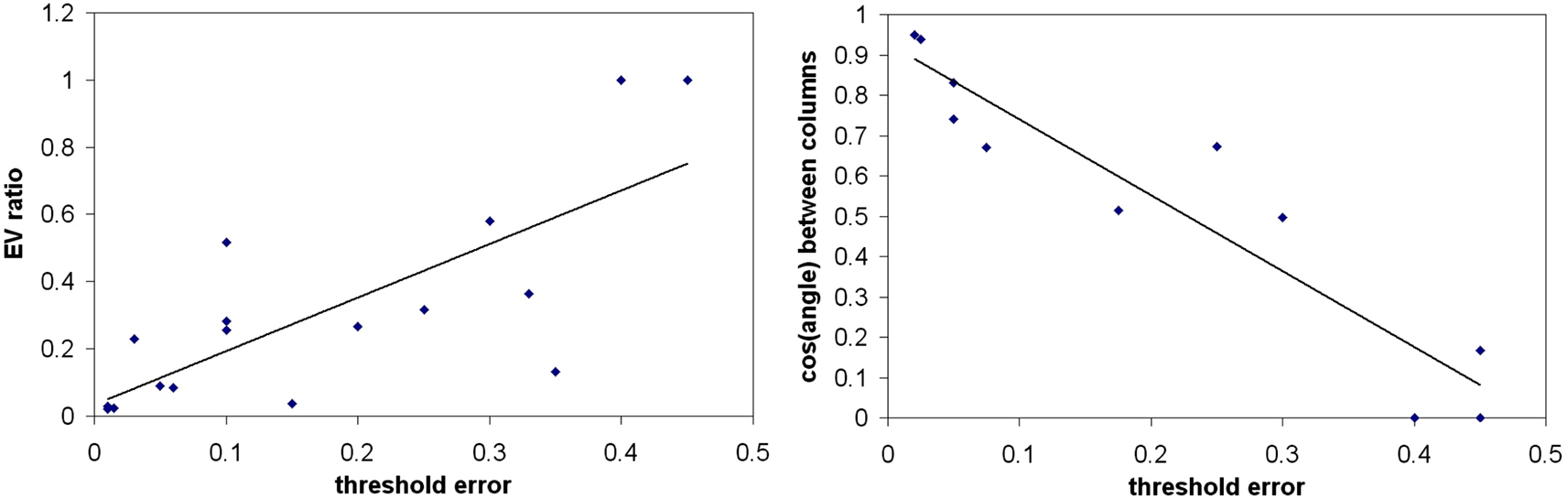
Figure 7. Relationship of increasing orthogonality of M with threshold error at which oscillations appear. Left figure shows a plot of the ratio of eigenvalues of MMT (λ2/λ1) against the threshold error bt for a given M, for various randomly-generated Ms selected to give a range of threshold errors. On the right hand side is a plot of bt (threshold error) against the cos(angle) between normalized columns of M (for the same set of random Ms). Note that for two exactly orthogonal Ms, different btvalues were obtained, n=2. The lines in both graphs are least squares fits.
The results in Figures 6 and 7
, using three different approaches, suggest that whitening the inputs make learning less crosstalk-sensitive, although the actual sensitivity varies unpredictably with the particular M used.
The source distribution was usually Laplacian, but some simulations were done with a logistic distribution (i.e. the distribution for which the nonlinearity is “matching”). The results were similar to those for the Laplacian distribution in terms of convergence to the ICs, but the onset of oscillation occurred at a threshold error rate that was about half that for the Laplacian case, using the same random mixing matrices (data not shown).
Hyvarinen–Oja One-Unit Rule
All the results described so far were obtained using the B-S multiunit rule, which estimates all the ICs in parallel, and uses an antiredundancy component to ensure that each output neuron learns a different IC. This antiredundancy component is rather unbiological, since it involves explicit matrix inversion, although crosstalk was only applied to the nonlinear Hebbian part of the rule. Although the antiredundancy component forces different outputs to learn different ICs, the actual assignment is arbitrary (depending on initial conditions and on the historical sequence of source vectors), though, in the absence of crosstalk, once adopted the assignments are stable. The results with this rule show 2 effects of crosstalk: (1) below a sharp threshold, approximately correct ICs are stably learned (2) above this threshold, learning becomes unstable, with weight vectors moving between various possible assignments of approximately correct ICs. Just over the crosstalk threshold, the weight vectors “jump” between approximate assignments, but as crosstalk increases further, the weights spend increasing amounts of time moving between these assignments, so that the sources can only be very poorly recovered. This behavior strongly suggests that despite the onset of instability the antiredundancy term continues to operate. Thus we interpret the onset of oscillation as the outcome of instability combined with antiredundancy. This leads to the important question of whether a qualitative change at a sharp crosstalk threshold would still be seen in the absence of an antiredundancy term, and what form such a change would adopt. We explored this using a form of ICA learning which does not use an antiredundancy term, the Hyvarinen–Oja one-unit rule (Hyvarinen and Oja, 1998
). This nonlinear Hebbian rule requires some form of normalization (explicit or implicit) of the weights, and that the input data be whitened. For simplicity we used “brute force” normalization (division of the weights by the current vector length), but similar results can be obtained using implicit normalization (e.g. as in the original Oja rule; Oja, 1982
).
A full account of these results will be presented elsewhere, and here we merely illustrate a representative example (Figure 8
), using seed 64 to generate the original mixing matrix M (n=2), which was then converted to an approximately orthogonal effective MO by multiplication by a whitening matrix Z derived from a sample of 1000 mix vectors obtained from Laplacian-distributed sources using M (see Materials and Methods and Appendix). There are two possible ICs (i.e. rows of MO) that the neuron can learn (in the absence of crosstalk), depending on the initial conditions; only one is shown here. Figure 8
shows the cosine of the angle between this IC and the weight vector (averaged over a window of 100,000 epochs after a stabilization period following changes in the crosstalk parameter). It can be seen that up to a threshold crosstalk value around 0.064 there is only a slight movement away from the correct IC. At this threshold the weight vector jumped to a new direction that was almost orthogonal to the original IC. The weight vector continued to fluctuate near this direction with no sign of oscillation. Although this direction was, in this case, quite close to the direction of the second possible IC, it seems unlikely that supratheshold crosstalk simply changes the IC that is learned (see Discussion). For example, we found similar behavior (n=3) using two Gaussian and one Laplacian sources. In this case there is only one stable IC to be found. In both cases (n=2 and n=3) when all sources were Gaussian (and therefore the mix signals have zero higher order cumulants so that ICA is not possible) the equilibrium weight vector shifted gradually as crosstalk increased (not shown), in the manner seen with a linear Hebbian rule (Radulescu et al., 2009
).
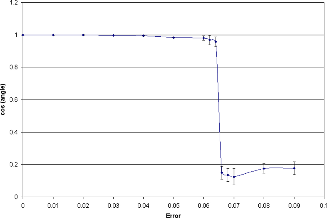
Figure 8. Effect of crosstalk on learning using a single-unit rule with N=2 and tanh nonlinearity. An orthogonal mixing matrix was constructed from seed 64 by whitening. The cosine of the angle between the IC found at 0 crosstalk (“error”) and that found at equilibrium in the presence of various degrees of crosstalk is plotted. This angle suddenly swings by almost 90° at a threshold error of 0.064 (E 0.113). The error bars show the standard deviation estimated over 100,000 epochs.
Biological Background
A synaptic connection has two main functions: it must convey selective information about the activity of the presynaptic neuron and its own current strength to the postsynaptic neuron, and it must appropriately adjust its strength based on the history of signals arriving at that connection. Both these operations should occur independently at different connections, even though the individual synapses comprising connections are very small and densely packed. Optimizing these related but different functions must be quite difficult, especially since they are somewhat contradictory: electrical signals must pass through the synapse towards a spike trigger region, while chemical signals must be confined to the synapse itself. Compartmentation is achieved by a combination of narrow spaces and buffering/pumping mechanisms. However, these strategies are themselves contradictory: chemicals that power pumps must arrive through the same narrow spaces. It is unlikely that connections operate completely independently of each other, even though there is little advantage in having large numbers of connections and neurons if they cannot. A central problem in neurobiology is the storage of information at very high density, as in other forms of computing (silicon or genetic), and neural information cannot be accurately stored unless connections change strength independently.
We are interested in the possibility that sophisticated brains use dual, direct and indirect, strategies to achieve high levels of connectional independence. Placing synapses on spines would be an example of a direct strategy. It is clear that the spine neck provides a significant, though not complete, barrier to calcium movement, and that calcium is a key chemical mediating activity-dependent modifications in synaptic strength (Wickens, 1988
; Lisman, 1989
; Muller and Connor, 1991
; Koch and Zador, 1993
; Lisman et al., 2002
; Nimchinsky et al., 2002
; Kampa et al., 2004
; Nevian and Sakmann, 2004
; Noguchi et al., 2005
; Feng et al., 2007
). We have proposed (Cox and Adams, 2000
; Adams and Cox, 2002a
,b
, 2006
) that the neocortex might in addition use an indirect, “Hebbian proofreading”, strategy, involving complex, mysterious but documented, microcircuitry that independently monitors and regulates activity at connections. However, while the suggestions that synapses cannot operate completely independently, and that the neocortex is partly a device for mitigating the effects of synaptic interdependence, are not inherently implausible, the key step in this argument has been missing: a demonstration that neural network learning fails if synapses are not sufficiently independent.
Any such failure would depend on the type of learning. We and others (Cox and Adams, 2000
; Adams and Cox, 2002a
,b
; Botelho and Jamison, 2004
; Radulescu et al., 2009
) have already shown that learning from pairwise correlations using a linear, but inaccurate, Hebb rule typically produces graceful degradation, with no sudden change at a critical error rate. However unsupervised learning by the neocortex probably requires sensitivity to higher-than-pairwise correlations since such correlations encode information about the underlying laws of nature, such as those transforming objects to images. We therefore studied the simplest model of such transformations: linear square deterministic mixing (i.e. the ICA model). This model has the attractive feature that learning by a single layer of feedforward weights is completely tractable (Dayan and Abbott, 2001
), at least with perfectly accurate Hebb synapses.
Physical Basis of Error and Nonlinearity
Although in at least some cases coincident activity at one synapse does affect adjustments at others on the same neuron (Engert and Bonhoeffer, 1997
; Bi, 2002
; Harvey and Svoboda, 2007
), the physical basis of such crosstalk is uncertain.
We briefly discuss this issue because mechanism affects magnitude, and it’s important to consider whether the magnitude of the crosstalk that leads to learning failure is consistent with experimental data. In at least one case (Tao et al., 2001
) crosstalk seems to be caused by dendritic diffusion of calcium. In a recent elegant study of crosstalk (Harvey and Svoboda, 2007
) evidence was obtained that crosstalk is caused by an “intracellular diffusible factor”. However, these authors suggests that this factor was not calcium, since in their experiments the calcium increase at a synapse caused by an LTP-inducing protocol at a neighboring synapse was only 1% (and not significantly different from 0%) of that occurring at that neighboring synapse. However, this reasoning may be flawed. First, that 1% signal is even less significantly different from 1% than it is from 0, and could double the calcium concentration at that synapse. Second, the space constant for the dendritic diffusion of the “factor” was similar to that measured for calcium diffusion (Noguchi et al., 2005
). Third, immediately following an LTP-inducing protocol at a spiny synapse, there is a dramatic decrease in the diffusional coupling of the spine head to the shaft (Bloodgood and Sabatini, 2005
), which would presumably prevent the escape of any “factor” (except for calcium itself, which is the earliest spine head signal, and which presumably triggers the uncoupling). Fourth, since LTP at a single synapse produces a stochastic, all-or-none increase in strength (Petersen et al., 1998
; O’Connor et al., 2005
), and to reliably induce LTP adequate stimuli must be presented many times [e.g. 30 stimuli over 1 min in the Harvey/Svoboda (Harvey and Svoboda, 2007
) experiments] it seems that some mechanism must “integrate” the magnitude of those stimuli over a minute-long time-window. An obvious “register” candidate for such integration is phosphorylation of CaM Kinase, the principal link between calcium and LTP expression (Lisman, 1990
; Derkach et al., 1999
; Lisman et al., 2002
). This means that repeated small increases in calcium at a synapse that are in themselves insufficient to trigger LTP, could nevertheless be registered at that synapse, and add to subsequent subthreshold calcium signals at that synapse to trigger all-or-none LTP. In the reverse protocol (Harvey and Svoboda, 2007
), where the subthreshold remote stimulus is given first, no threshold change is seen, possibly because the observed spine structural changes shield the synapse from subsequent small dendritic calcium signals.
One possible objection to this argument would be that very small changes in calcium may fail to affect the register, for example if calcium activates CaM Kinase nonlinearly (De Koninck and Schulman, 1998
). This raises the important question of the possible biophysical basis of the nonlinearity that is essential for learning high-order statistics. There are two possible limiting cases. (1) “nonlinearity first”: the nonlinearity is applied to the Hebbian update before part of that update leaks to other synapses. This is the form we adopted in this paper (Eq. 2). In this case the nonlinearity might reflect a relation between depolarization and spiking, or between spike coincidence and calcium entry. (2) “nonlinearity last”: the calcium signal would linearly relate to the number of coincidences; after attenuation it would then be linearly distributed to neighboring synapses, where it would nonlinearly combine with whatever other calcium signals occur at those synapses. This would lead to an equation of form:

We will describe the behavior of this case in another paper, but it seems to be similar to that described here.
Clearly in the “nonlinearity first” case, the register would respond linearly to calcium (as assumed in our derivation of b). In the “nonlinearity last” case, the register could perhaps discriminate against very small calcium signals emanating from neighboring synapses; however, the effectiveness of such a mechanism would be constrained by the requirement to implement a nonlinearity that is suitable for learning, and not just for discrimination against stray calcium. An extreme case of a nonlinearity would be a switch from LTD to LTP at a threshold (Cooper et al., 2004
). Thus if calcium spreads, LTP at one synapse might cause LTD at neighboring synapses. However, we found that making the offdiagonal elements in E negative did not substantially affect the onset of instability.
None of our results hinge on the nature of the diffusing crosstalk signal. However, if we assume it is calcium, we can try to estimate the magnitude of possible biological crosstalk, and compare this to our range of values of bt, to see whether our results might be biologically significant. There are two possible approaches. The first is based on detailed realistic modeling of calcium diffusion along spine necks, including buffering and pumping. Although indirect, such modeling does not require the use of perturbing calcium-binding dyes. Zador and Koch (1994)
have estimated that about 5% of the calcium entering through the NMDAR might reach the dendritic shaft (most of the loss would be due to pumping by the spine neck membrane). How much of that 5% might reach neighboring spine heads? Obviously simple dilution of this calcium by the large shaft volume would greatly attenuate this calcium leakage signal, and then the diluted signal would be further attenuated by diffusion through a second spine neck. It might seem impossible that after passing this triple gauntlet (neck, dilution, neck) any calcium could survive. However, one must consider that the amount of stray calcium reaching a particular spine head reflects the combined contribution of stray signals from all neighboring spines: it will depend on the linear density of spines. One way to embody this was outlined in Methods. Another even simpler approach was adopted by Cornelisse et al. (2007)
: they pointed out that in the case where all synapses are active together (perhaps a better approximation than that only one is active at a time) one could simply regard each spine as coupled to a shaft segment that was as long as the average distance between spines. Typically, this segment volume is comparable to the spine head volume, so the “dilution factor” would only be around twofold. Furthermore the effect of neck pumps on calcium transfer from shaft to head will be much less than that on transfer from head to shaft, because the spine head does not have a large volume relative to the relevant dendritic segment. Indeed, the extra head-head attenuation produced by dilution is offset by the reduced head-head attenuation due to finite head volume. The underlying cause is the different boundary condition for head-shaft and shaft-head reaction-diffusion. Making necks longer or narrower could improve isolation, but would lead to decreased electrical effectiveness for single synapses, requiring compensating increases in synapse numbers and no net decrease in crosstalk.
The second approach is direct measurement using fluorescent dyes. Such dyes inevitably perturb measurements, and this field has been very controversial, with one group claiming that under natural conditions there is negligible loss to the shaft (Sabatini et al., 2002
) and other groups arguing that there can be low but significant loss (Majewska et al., 2000
; Korkotian et al., 2004
; Noguchi et al., 2005
). On balance these studies suggest that natural loss is in the range 1–30%. A very conservative overall figure of 1% for head-shaft attenuation and 10% for shaft-head attenuation, giving a combined a value of 10−3, is used below. It should be noted that even if calcium is not the source of crosstalk (Harvey et al., 2008
), our results still hold. Furthermore, even though such diffusion is a local, intersynapse, phenomenon, it will affect the specificity of adjustments of connections in a global manner, both because feedforward connections are often comprised of many synapses distributed over the dendritic tree (Markram et al., 1997
), and because synapses typically form and disappear at many locations (Kalisma et al., 2005
; Le Be and Markram, 2006
; Keck et al., 2008
). Although most of our results were obtained assuming, for simplicity, that all connections affect each other equally (which would only be true in the limits that each connection is made of very many synapses, or that learning is slow compared to the turnover of individual synapses (or, a fortiori, both), we found the same qualitative behaviour using error matrices with randomly varying offdiagonal elements. The way that local synapse crosstalk could lead to global connection crosstalk is further detailed in our paper on linear learning (Radulescu et al., 2009
).
Crosstalk Triggers Instability in the BS Model
We studied the role of error in the BS model of ICA, an extensively studied learning paradigm in neural networks (Bell and Sejnowski, 1995
; Hyvärinen et al., 2001
). Figure 2
shows that the performance of the ICA network is at first only slightly degraded when minor error is introduced. It appears that the effect of minor crosstalk is that a slightly degraded version of M−1 is stably learned, as one might expect. This result is related to what we see with linear Hebbian learning: the erroneous Oja rule (Oja, 1982
) learns not the leading eigenvector of the input covariance matrix C, but that of EC (Adams and Cox, 2002a
; Botelho and Jamison, 2004
; Radulescu et al., 2009
). However, in the linear case, stable (though increasingly degraded) learning occurs all the way up to the trivial error rate. It appears that in the present, nonlinear, case, at a threshold error rate below the trivial value a qualitatively new behaviour emerges: weight vectors become unstable, shifting between approximately correct solutions, or, in the one-unit case, showing dramatic, but stable, shifts in direction. In particular, just above the error threshold, the weight vectors “jump” unpredictably between the possible (approximately correct) assignments that were completely stable just below the threshold (see Appendix). These jumps appear to be enabled because, at the threshold, one of the weights spends long periods near 0, with occasional brief sign reversals. As a weight goes through 0, it becomes possible for the direction of the weight vector to dramatically change during unusual short pattern runs, even though the weights themselves can only change very slightly (because the learning rate is very small). In particular, the weight vectors are able to swing to alternative assignments to rows of M−1. Furthermore, the weight vectors can also remain aligned to their current assignments, but swing through 180°, by a change in sign (see Appendix). This means that exactly at the error threshold, the “orbit” consists of almost instantaneous jumps between corners of a parallelogram, followed by protracted sojourns at a corner. This parallelogram rounds out to an ellipse as error increases, with the weight vectors spending increasingly longer periods away from approximately correct assignments, so that the network recovers the sources increasingly poorly.
These oscillations could be viewed as a manifestation of the freedom of the BS rule to pick any of the possible permutations of M−1 that allow source recovery, and if we had measured performance using the customary Amari distance (Amari et al., 1996
) which takes into account all possible assignments, the sudden onset of instability would be concealed. An extreme case would be if weights instantaneously jumped between various almost correct assignments, as seems to happen exactly at the error threshold (see Appendix Results): there would be no sudden change in the Amari distance and within the strict ICA framework, any W that allows sources to be estimated is valid. Such jumps are usually never seen in the absence of error, and to our knowledge such behavior has never been reported (though we have observed approximately this behavior in error-free simulations using high learning rates, which are of course very noisy). At higher learning rates (Figure 2
) or for error rates well beyond bt (Figure 4
A), the network spends relatively more time relearning a progressively less accurate permuted version of M−1, so the Amari distance (averaged over many epochs) would decline further.
It should be noted that although the detailed results we present above were obtained using the original BS rule, in which a matrix-inversion step is used to ensure that different output neurons find different ICs, an apparently related failure above a threshold error rate is also seen with versions of the rule (Amari, 1998
; Hyvarinen and Oja, 1998
) that do not use this feature (e.g. Figure 8
). When only a single output neuron is used, with an orthogonal mixing matrix, jumping between approximate ICs may not be possible. Instead, we find that at a threshold crosstalk value, the rule fails to find, even approximately, the initially selected IC, and jumps to a new direction. While in some cases this new direction happens to corresponds to another possible IC, this is probably coincidental: it remains in this direction as crosstalk further increases, and in some cases that we tested all the other possible ICs are unstable (because they correspond to Gaussian sources). Clarification of the significance of the suprathreshold direction requires further work.
Thus in both versions of ICA learning there is a sharp deterioration at a threshold error, making the rules more or less useless, though the form of the deterioration varies with the form of the rule.
The Dynamical Behaviour of the BS Rule with Error
Our results are merely numerical, since we have been unable to extend Amari’s stability analysis to the erroneous case. The following comments are therefore only tentative.
The behaviour seen beyond the threshold error rate may arise because the fixed points of the dynamics of the modified BS rule, i.e. degraded estimates of permutations of M−1, become unstable. The behavior in Figures 2
, 3 and 4
A resembles a bifurcation from a stable fixed point to a limit cycle, the foci of which correspond approximately to permutations of M−1. Although we suspect that this is the case, we have not yet proved it, since it is difficult to write an explicit expression for the equilibria of the erroneous rule, a necessary first step in linear stability analysis. Presumably Amari’s stability criterion must be modified to reflect both M and E. The fact that the onset of oscillations occurs at almost 0 frequency suggests the bifurcation may be of the “saddle-node on invariant circle” variety, like Hodgkin class 1 excitability (Strogatz, 2001
; Izhikevich, 2007
). Figures 5
A,B shows that when n = 5 more complex behaviour can occur for error beyond the threshold level. We see that one of the rows of W seems to wander irregularly, not visiting any IC for millions of epochs. We do not know if this behavior reflects a complicated limit cycle or chaos, but from a practical point of view this outcome would be catastrophic. In a sense the particular outcome we see, onset of oscillations at a crosstalk threshold, is a peculiarity of the form of the rule, in particular the operation of the rather unbiological antiredundancy term. Nevertheless, even though the antiredundancy term operates accurately and effectively, the compromised accuracy of the Hebbian term no longer allows stable learning. In another version of ICA, the Oja–Hyvarinen single unit rule, there is no antiredundancy term, yet IC learning still fails at a sharp threshold (Figure 8
).
Whitening
Most practical ICA algorithms use whitening (removal of pairwise correlations) and sphering (equalizing the signal variances) as preprocessing steps. In some cases (e.g. Hyvarinen and Oja, 1998
) the algorithms require that M be orthogonal (so the mixed signals are pairwise uncorrelated). As noted above it is likely that the brain also preprocesses data sent to the cortex [e.g. decorrelation in the retina and perhaps thalamus (Srinivasan et al., 1982
; Atick and Redlich, 1990
, 1992
)], and we explored how this affects the performance of the inaccurate ICA network. Whitening the data did indeed make the BS network more robust to Hebbian error as Figures 6 and 7
show, with the onset of instability occurring at higher error levels as the data were whitened more. However, even for completely orthogonal Ms, oscillations usually still appear at error rates below the “trivial value” εt, for which learning is completely inspecific (εt=(n − 1)/n). As discussed further below, if synapses are very densely packed, even error rates close to the trivial rate could occur in the brain.
Neither for random nor orthogonal Ms could we predict exactly where the threshold error would lie, although it is typically higher in the orthogonal case (Figures 6 and 7
). Some, but not all, of the variation in the bt values could be explained by the degree of nonorthogonality of M, estimated in two different ways. First, for an orthogonal matrix multiplication by its transpose yields the identity matrix, which has all its eigenvalues equal; we found that the bt for a given random M was correlated with the ratio of the first two eigenvalues of MMT (Figure 7
, left). Second, if the columns of a matrix whose columns are orthogonal have equal length (i.e. the matrix is orthogonal), so do the rows. When we normalized the columns of a given random M, we found an improved correlation between the cosine of the angle between the columns and bt (Figure 7
).
Another factor influencing the threshold error rate for a given M was the source distribution; we found that the threshold error rate was typically about halved for logistic sources compared to Laplacian, despite the fact that this improves the match between the nonlinearity and the source cdf. We suspect that this is because the kurtosis is lower for the logistic distribution (1.2 compared to 3 for the Laplacian).
Even though learning can tolerate low amounts of error in favorable cases (particular instances of M and/or source distributions), low biological error can only be guaranteed by using small numbers of inputs. In the neocortex the number of feedforward inputs that potentially synapse on a neuron in a cortical column often exceeds 1000 (Binzegger et al., 2004
), so b values would have to be well below 10−3 to keep total error below the trivial value, and considerably less to allow learning in the majority of cases. In the simple model summarized in the Methods, which assumes that strengthening is proportional to calcium, which diffuses along dendrites, we obtained b=2αaλc/L. a is the effective calcium attenuation from one spine head to another when both are at the same dendritic location; a factor that the preceding discussion suggests cannot be much below 10−3. α is typically around 10 for feedforward connections (Binzegger et al., 2004
), λc around 3 μm (Noguchi et al., 2005
) and L around 1000 μm (Binzegger et al., 2004
), so nb would be around 6 × 10⁻², which often produces breakdown for Laplacian sources. If the cortex were to do ICA (perhaps the most tractable form of nonlinear learning), it would require additional, error-prevention machinery, especially if input statistics were less rich in higher order correlations than in our Laplacian simulations (see below). If the cortex uses more sophisticated strategies (because inputs are generated in a more complex manner than in ICA), the problem could be even worse.
The fact that whitening can make the learning rule more error-resistant suggests at first sight that our study has only theoretical, not practical, significance, because whitening is a standard process which digital computers can accurately implement. However, the brain is an analog computer (albeit massively parallel) and so it cannot whiten perfectly, because whitening filters cannot be perfected by inaccurate learning. While learning crosstalk does not produce a qualitative change in the performance of the Oja model of principal components analysis (unlike the ICA model studied here), it does degrade it, especially when patterns are correlated (Adams and Cox, 2002a
; Botelho and Jamison, 2004
; Radulescu et al., 2009
).
Crosstalk and Clustering
In the ICA model completely accurate Hebbian adjustment leads (within the limit set by the learning rate) to optimal learning, which is degraded (above a threshold, quite dramatically) by “global” crosstalk. However, other authors have suggested that a local form of crosstalk could instead be useful, by leading to the formation of dendritic “clusters” of synapses carrying related information. In particular, it has been suggested that with such clustered input excitable dendritic segments could function as “minineurons”, so that a single biological neuron could function as an entire multineuron net (Hausser and Mel, 2003
; Larkum and Nevian, 2008
; Polsky et al., 2008
), with greatly increased computational power. While these are intriguing suggestions, they seem unlikely to apply to the neocortex, which is the ultimate target of our approach. While crosstalk between synapses is clearly local, cortical connections are typically composed of multiple synapses scattered over the dendritic tree (e.g. Markram et al., 1997
), so crosstalk between connections is likely to be more global. We know of no evidence for such clustering in the neocortex. Furthermore, such clustering may not always confer increased “computational power”, at least in the following restricted sense: a biological neuron with clustered inputs and autonomous dendritic segments could indeed act as a collection of connectionist “neuron-like” elements but these elements could not have as many inputs as a whole biological neuron, simply because there would not be as much available space on a segment as on the entire tree. In particular, in the case of correlation-based Hebbian learning, there would be no net computational advantage, and indeed for learning from higher-order correlations there would be decided disadvantages. Thus for linear learning, learning by segments would only be driven by a subset of the overall covariance matrix for the total input set; correlations between the activities of these segments could then also be explored (for example at branchpoints) but the net result could only be that learning by the entire neuron would be driven by the overall covariance matrix, with no net computational advantage. But for nonlinear learning driven by higher-order correlations, clustering and segment autonomy would simply vastly restrict the range of relevant higher-order correlations, since only higher-order correlations between subsets of inputs could be learned.
The crux of the argument we are attempting to make in this paper is that real neurons cannot be as powerful as ideal neurons, since the former must exhibit crosstalk, which sets a fundamental barrier to the number of inputs whose HOCs a neuron can usefully learn from. Furthermore, the essence of the problem the brain faces is to make intelligent choices based on a learned internal model of the world, which must be constructed using nonlinear rules operating on the HOCs present in the multifarious stimuli the brain receives. The power of the model a neuron learns depends on the number of inputs, and the number of learnable inputs is set by (biophysically inevitable) crosstalk. Therefore a fundamental difficulty intelligent brains face is (given that the learning problems themselves are endlessly diverse), making sure connection adjustments occur sufficiently accurately. In this view the problem is not that the brain does not have enough neurons, but that neurons cannot have enough inputs. Obviously our limited numerical results with toy models cannot establish this conclusion, but they do support it, and since this viewpoint is both powerful and novel, we feel justified in sketching it here. Even more generally, it seems likely that the combinatorial explosions which bedevil difficult learning problems cannot be overcome using sufficiently massively parallel hardware, since massive parallelism requires analog devices which are inevitably subject to physical errors.
Learning in the Neocortex
How could neocortical neurons learn from higher-order correlations between large numbers of inputs even though their presumably nonlinear learning rules are not completely synapse-specific? The root of the problem is that the spike coincidence-based mechanism which underlies linear or nonlinear Hebbian learning is not completely accurate: coincidences at neighboring synapses affect the outcome. In the linear case, this may not matter much (Radulescu et al., 2009
) but in the nonlinear case our results suggest that it could be catastrophic. Of course our results only apply to the particular case of ICA learning, but because this case is the most tractable, it is perhaps all the more striking. Other nonlinear learning rules have been proposed based on various criteria (e.g. Dayan and Abbott, 2001
; Hyvärinen et al., 2001
; Cooper et al., 2004
; Olshausen and Field, 2004
) and it will be interesting to see whether these rules also fail at a sharp crosstalk threshold.
Other than self-defeating brute force solutions (e.g. narrowing the spine neck), the only obvious way to handle such inaccuracy is to make a second independent measure of coincidence, and it is interesting that much of the otherwise mysterious circuitry of the neocortex seems well-suited to such a strategy. If two independent though not completely accurate measures of spike coincidence at a particular neural connection (one based on the NMDAR receptors located at the component synapses, and another performed by dedicated specialized “Hebbian neurons” which receive copies of the spikes arriving, pre- and/or postsynaptically, at that connection) are available, they can be combined to obtain an improved estimate of coincidence, a “proofreading” strategy (Adams and Cox, 2006
) analogous to that underpinning Darwinian evolution (Swetina and Schuster, 1982
; Eigen, 1985
; Leuthausser, 1986
; Eigen et al., 1989
). The confirmatory output of the coincidence-detecting Hebbian neuron would have to be somehow applied to the synapses comprising the relevant connection, such that the second coincidence signal would allow the first (synaptic) coincidence signal to actually lead to a strength change. While direct application (via a dedicated modulatory “third wire”) seems impossible, an effective approximate indirect strategy would be to apply the proofreading signal globally, via two branches, to all the synapses made by the input cell and received by the output cell; the only synapses that would receive both, required, branches of the confirmatory feedback would be those comprising the relevant connection (in a sufficiently sparsely active and sparsely connected network; Olshausen and Field, 2004
). We have suggested that layer 6 neurons are uniquely suited to such a Hebbian proofreading role, since they have the right sets of feedforward and feedback connections (Adams and Cox, 2002a
, 2006
).
In summary, our results indicate that if the nonlinear Hebbian rule that underlies neural ICA is insufficiently accurate, learning fails. Since the neocortex is probably specialized to learn higher-order correlations using nonlinear Hebbian rules, one of its important functions might be reduction of inevitable plasticity inspecificity.
Methods
Generation of random vectors
To get a vector of which each element is drawn from a Laplacian distribution, first an N element vector s, the elements of which is drawn from a uniform distribution (range{−0.5,0.5}), is generated by using the Matlab rand function: s=−0.5 + [0.5 − (−0.5)] * rand(1,N). Then each element si of x is then transformed into a Laplacian by the following operation:
si=−sign(si)ln(1 − 2|si|)
“sign” means take the variable xi and if it is positive, assign it the value 1, if it is negative assign it the value −1, and if 0 assign it the value 0.
Mixing matrices used in the simulations
The mixing matrix M used for Figure 2
was  (rand seed 8, {0,1}) and for Figure 4
was
(rand seed 8, {0,1}) and for Figure 4
was  (rand seed 10, {0,1})
(rand seed 8, {0,1}) and for Figure 4
was (rand seed 10, {0,1})The mixing matrix (seed 8) used in Figure 5
was
Orthogonality
Perturbations from orthogonality were introduced by adding a scaled matrix (R) of numbers (drawn randomly from a Gaussian distribution) to the whitening matrix Z. The scaling factor (which we call “perturbation”) was used as a variable for making MO (see Orthogonal Mixing Matrices) less orthogonal, as in Figure 5
. Below are the matrices used in generating one of the data sets of Figure 5
with M generated from seed 8 (seeds 2–6 were used to generate the different R matrices for the five data sets in Figure 5
):
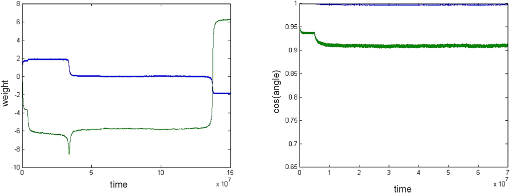
Figure A1. On the left is a plot of the weights of one of the rows of W with error of 0.0088 (i.e. just above the apparent threshold error) applied at 4 M epochs at γ=0.0005 (seed 10). These are the weights comprising the “other” weight vector from the one whose behavior was shown in Figures 4
B,C. Thus the large swing in the weight vector shown in Figures 4
B,C produced relatively small adjustments in the weights shown here ( at 30 M epochs), while the very large weight changes shown here (at 140 M epochs) correspond to small shifts in the direction of the weight vector shown in Figures 4
B,C. (Conversely, these large weight steps at 140 M epochs produce a spike-like swing in the corresponding weight vector angle). Note the weights make rapid steps between their quasistable values. Also the smaller (blue) weight spends a very long time close to 0 preceding the large weight swing (during which swing the weight vector goes briefly and almost simultaneously orthogonal to both rows of M−1). Close inspection revealed that the blue weight crosses and recrosses 0 several times during the long “incubation” period near 0. Note the wobbly appearance of the green weight. The thickness of the lines in the left and right plots reflects rapid small fluctuations in the weights that are due to the finite learning rate. On the right is the plot of the cos(angle) between the weight vector whose components are shown in the left plot, and the two rows of M−1. However, b=0.00875 (i.e. very close to the error threshold; see Figure A2
) introduced at 5 M epochs;other parameters the same as in the left plot. Note that the weight vector relaxes from the correct IC to a new stable position corresponding to a cos angle just below 1 (blue plot), and then stays there for 65 M epochs. The relaxation is more clearly seen in the green plot, which shows the cos angle with the row of M−1 that was not selected.
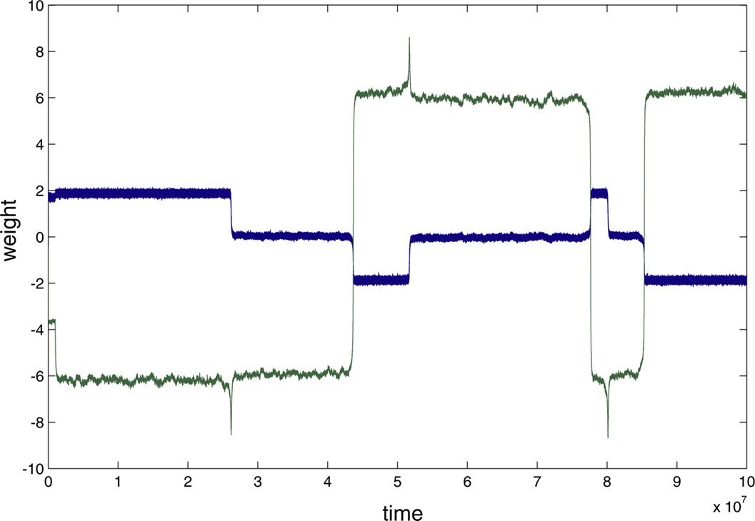
Figure A2. Plots of individual rates using the same parameters as in Figure A1 except γ=0. 005 (which increases the size of the slow and fast fluctuations, which is why the lines are thicker than in Figure A1
) and b=0.0087 (which appears to be extremely close to the true error threshold for this M; the first oscillations occurs at 27 M epochs, which would correspond to 270 M epochs at the learning rate used in Figure A1
), introduced at 1 M epochs. Each weight (i.e. green and blue lines) comprising the weight vector adopts four possible values, and when the weights step between their possible values they do so synchronously and in a particular sequence (though at unpredictable times). The four values of each weight occur as opposite pairs. Thus the green weight occurs as one of four large values, two positive and two equal, but negative. The two possible positive weights are separated by a small amount, as are the two possible negative weights. The blue weight can also occupy four different, but smaller values. Thus there are two small, equal but reversed sign weights, and two even smaller equal but reversed sign weights. These very small weights lie very close to 0. Since the weights jump almost synchronously between their four possible values, the “orbit” is very close to a parallelogram, which rounds into an ellipse as error increases. One can interpret the four corners of the parallelogram as the four possible ICs that the weights can adopt: the two ICs that they actually do adopt initially and the two reversed sign ICs that they could have adopted (if the initial weights had reversed sign). However, two of the corners are closer to correct solutions than are the others (corresponding to the assignment reached when the blue weights are very close to 0). It seems likely that exactly at the error threshold the difference between the two close values of the green weights, and the difference between the very small values of the blue weights, would vanish. This would mean that the blue weights would be extremely close to 0 during the long period preceding an assignment swap, so the direction of the weight vector would be very sensitive to the details of the arriving patterns. Consistent with this interpretation, the weights fluctuate slowly during the long periods preceding swaps; these fluctuations, combined with the vanishing size of one of the weights, presumably make the system sensitive to rare but special sequences of input patterns. Similar behavior was seen using seed 8.
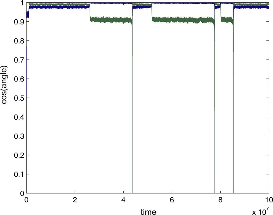
Figure A3. This shows the behavior of the weight vector whose component weights are shown in Figure A2 (cos angle with respect to the two rows of M−1) Error b=0. 0087 introduced at 1 M epochs. Note the weight vector steps almost instantaneously between its two possible assignments. However, when the weight vector is at the blue assignment, it is closer to a true IC than it is when it is at the green assignment (which is the assignment it initially adopts. When the weight vector shifts back to its original assignment (at 43 M epochs), it shifts orthogonal to both ICs at almost the same moment (sharp downspikes to 0 cosine). Notice the extreme irregularity of the “oscillations”.
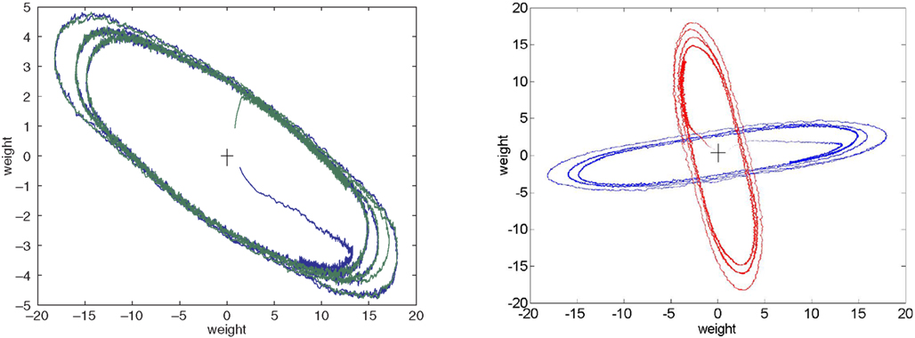
Figure A4.The plot on the right is similar to those of Figure 3 except that the data was generated from a different simulation with all parameters being the same except that the initial weight vectors were different. Notice how one of the weight vectors (rows of W) initially evolves to the mirror image in terms of sign of the weight vector in Figure 3
A (right most red blob). The right hand plot shows weight 1 from row 1 of W with weight 2 of row 2 (blue) and weight 2 of row 1 with weight 1 of row 2 (red).
 (from seed 2)
For instance the matrix at perturbation=0.5 on the graph would be MO=(0.5R + Z)M.
This procedure resulted in each element of MO being altered by an amount in the range (0–25%) as the perturbation ranged from between (0–1.5).
One-unit Rule
The whitened matrix used in the simulations for Figure 8
was:
Results
Plots near the error threshold
Figure 4
B showed a 150 M epoch simulation using seed 10 for M b = 0.0088 and γ=0.0005 During the oscillation “spikes” one of the weight vectors moves almost exactly orthogonal to both of the rows of M−1. This can only happen if both weights go through 0 at the same moment. Closer inspection revealed however that there is a slight delay (on the order of 10 K epochs) between the moments that these vectors swing through 90°, such that the 2 weights do not 0 at exactly the same moment. Preceding the swings, one of the weights spends very long periods hovering near 0. At these very low learning rates, the weight vector spends extremely small amounts of time near any of the rows of M−1.
The authors declare that the research was conducted in the absence of any commercial or financial relationships that could be construed as a potential conflict of interest.
We thank Larry Abbott and Terry Elliott for their comments on the manuscript, and to Miguel Maravall for discussions and input on an earlier draft.
Adams, P. R., and Cox, K. J. A. (2006). A neurobiological perspective on building intelligent devices. Neuromorphic Eng. 3: 2–8 Available at: http://www.ine-news.org/view.php?source=0036-2006-05-01
.