1
Department of Physiology, Northwestern University, Chicago, IL, USA
2
Department of Neuroscience and Brain Technologies, Italian Institute of Technology, Genova, Italy
3
Department of Biological Sciences, University of Illinois at Chicago, Chicago, IL, USA
4
Department of Biomedical Engineering, Northwestern University, Chicago, IL, USA
5
Rehabilitation Institute of Chicago, Chicago, IL, USA
A critical advance for brain–machine interfaces is the establishment of bi-directional communications between the nervous system and external devices. However, the signals generated by a population of neurons are expected to depend in a complex way upon poorly understood neural dynamics. We report a new technique for the identification of the dynamics of a neural population engaged in a bi-directional interaction with an external device. We placed in vitro preparations from the lamprey brainstem in a closed-loop interaction with simulated dynamical devices having different numbers of degrees of freedom. We used the observed behaviors of this composite system to assess how many independent parameters − or state variables − determine at each instant the output of the neural system. This information, known as the dynamical dimension of a system, allows predicting future behaviors based on the present state and the future inputs. A relevant novelty in this approach is the possibility to assess a computational property – the dynamical dimension of a neuronal population – through a simple experimental technique based on the bi-directional interaction with simulated dynamical devices. We present a set of results that demonstrate the possibility of obtaining stable and reliable measures of the dynamical dimension of a neural preparation.
We report a new approach to identifying the dynamical properties of neural tissue engaged in a bi-directional interaction with an external device. We developed a brain–machine interface (BMI) system, where the dissected brain of lamprey larvae was connected bi-directionally with an external dynamical system (EDS). While BMIs are mostly applied to clinical conditions, such as complete paralysis or loss of some senses, here we consider an application to the study of the computational properties of neural systems. One can distinguish between (i) motor BMIs, where a direct communication pathway is established from the nervous system to an external device (Donoghue, 2008
; Hochberg et al., 2006
); (ii) sensory BMIs, where a direct communication pathway is established from an external device, e.g. an artificial retina, to the nervous system (Counter, 2008
; Dowling, 2005
; Mokwa, 2007
); and (iii) bi-directional BMIs, where a bi-directional direct communication is established between the nervous system and an external device (Bakkum et al., 2007
; Karniel et al., 2005
; Martinoia et al., 2004
). The setup describe in this paper is an example of a bi-directional BMI.
The sensory information about the current state of the external system was conveyed to the neural preparation by means of electrical pulse trains of variable frequencies, delivered by tungsten electrode. Population spike trains extracted in real time from extracellular multiunit recording were transformed into a control signal used to drive the external system. In engineering terms, this is called a closed-loop configuration (Bakkum et al., 2008
; Chao et al., 2008
; Novellino et al., 2007
), as the sensory consequences of the control signals are fed-back to the control system to generate new commands. From a mathematical standpoint, when the external input is maintained constant, such a closed-loop system approximates an “autonomous system” whose dynamics are entirely self-contained and do not depend explicitly upon time. Of course, this is only an approximation, as external influences, such as the fluctuation of temperature in the room, are most likely to affect the system’s behavior.
In this experimental setting, as in any BMI, the dynamics of the neural component are of critical importance in governing the motions of the external system. These dynamics determine whether the output of the neural preparation depends only on the current sensory or artificially delivered input or also on some internal process within the central nervous system itself. The question addressed by this study is how many independent parameters − or state variables − determine at each instant the output of the neural system. This information is known as the “dynamical dimension” (Janjarasjitt et al., 2008
; Shen et al., 2003
; Theiler and Rapp, 1996
) and is related to the capacity of a neural population to generate complex patterns of activity, which may be used as control signals for external devices.
The most critical and innovative feature of the proposed method is the use of an external device with programmable dynamical properties as a research tool for studying the dynamical properties of the neural preparation. The closed-loop interaction with the device facilitates the identification of specific computational features, such as the dynamical dimension, through the creation of a BMI system capable of generating autonomous behaviors. These are behaviors that do not require the application of external inputs, whose design involves a significant amount of complexity and arbitrariness in more traditional system identification methods.
General Paradigm
We consider the bi-directional signal exchange between a neural system and an external device as a means to get at the neural preparation’s dynamical dimension. We measured the dynamical dimension of the preparation embedded within the closed-loop BMI system shown schematically in Figure 1
. The term “neural preparation” refers to the part of the nervous system that affects the recorded signal. In general mathematical terms, the external system is described by the state and output equations:
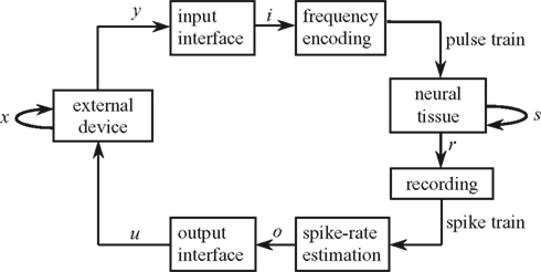
Figure 1. Experimental paradigm. The box representing the neural tissue has two incoming arrows: one is a recurrent arrow and represents the state s, the other represents the input signal i, which is conveyed using frequency encoding. The signal recorded by the extracellular electrode contains information about the state s in the form of population spike train. The spike train is converted into a sequence of estimated spike rates, which serve as an output signal o from the tissue. The box representing the external device has two incoming arrows, like the neural tissue box. The change in state of the external device, x, depends only upon the current state and the control signal u (Eq. 1).
Here, x is the state of the external device, u is a control signal, y is the read-out signal, h and p are arbitrary functions, and the subscripts refer to discrete sampling time.
One can describe in the same way the neural preparation as a dynamical system. The main assumption of our study is that there exists a state representation (s) of the neural preparation such that the changes of state are completely determined by the state itself and by the input to the neural preparation:
Here, i and o refer to the input and output of the neural preparation. Both s and x are vectors. In principle, there may be infinitely many equally valid representations for s. However, its dimension (the dynamical dimension), that is the number of independent components in any numerical representation of s, is a well-defined property of the preparation, which we seek to determine.
The neural preparation and the external device are interconnected in a closed-loop through two instantaneous mappings:
By combining these relations with the dynamics of both the external system and the neural preparation (Eqs 1–3) one obtains a single equation:

where q = [x, s]T is the state of the composite system and is a composition of the states of the two sub-systems, the external device and the neural preparation, and:
Accordingly,

This equation does not hold true in the general case. It can be violated due to degeneration of the composite system into lower order. The assessment of the dynamical dimension of the neural component can also be adversely affected by (i) significant difference between natural frequencies of the neural component and the external system, and (ii) by input signals driving the neural component into saturation. We have analyzed each of these possible causes and investigate how to avoid each of them. An extensive discussion of this issue can be found in the Supplementary Material.
By construction, the behavior of the composite system does not depend on any external input, but only on its current state: this is the defining property of an “autonomous system.” In any practical case, autonomy must be understood as an approximation, because uncontrolled external inputs cannot be entirely discounted. We assessed the dynamical dimension of the composite system, dim(q), by collecting multiple trajectories of the external device. Then, we computed the dynamical dimension of the neural preparation, dim(s), from Eq. 6, by subtracting the known dimension of the external system, dim(x), from the estimated dimension of the combined system:

The main element of novelty with this approach consists in the possibility of using external systems with different dimensions. Then, it is possible to use the known difference between the dimensions of the external systems as condition to validate the estimate of the dimension of the neural preparation. This provides us with a critical tool, as the estimate of a system’s dimension is typically affected by noise and by arbitrariness in some data-processing parameters.
The Neural Preparation and the Experimental Setup
The whole brain of the Sea Lamprey was dissected and maintained in continuously superfused Ringer’s solution (see details in Alford et al., 1995
; Karniel et al., 2005
). The dissected neural tissue was maintained alive for up to several days. Figure 2
shows the preparation in the recording chamber.
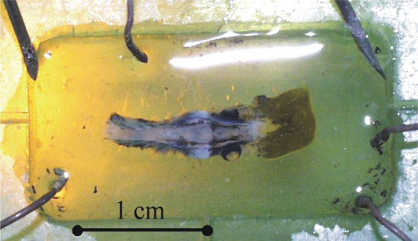
Figure 2. The lamprey. The neural element of the BMI system is the dissected brain of Sea Lamprey maintained alive within the recording chamber.
The stimulating electrode was placed among the axons of the vestibulo-reticular pathway, which originates from one of the posterior octavomotor nuclei (nOMP). This nucleus receives inputs from the vestibular capsule and its axons form synapses with the contralateral rhombencephalic neurons.
The recording electrode was placed extracellularly among the axons of the (contralateral) reticulo-spinal pathway, originating from the posterior rhombencephalic reticular nucleus (PRRN). This nucleus received monosynaptic projections from the contralateral nOMP. In behaving animals, the PRRN conveys sensory information of different nature (visual, vestibular, tactile) and central commands to the motor centers of the spinal cord (Rovainen, 1979a
,b
). This placement of the stimulation and recording electrodes induces predominantly excitatory responses (Alford et al., 1995
).
The recorded signals were acquired at 10 kHz by a data acquisition board (National Instruments PCI-MIO-16E4) on a Pentium III 2GHz computer (Dell Computer Corporation). The recording/stimulating paths from the workstation to the tissue followed the subsequent scheme. The recording electrode (a glass micropipette filled with 1 M NaCl, impedance range 1–10 MΩ) was connected to a pre-amplifier within a Faraday cage which was in turn connected to an external amplifier. The stimulator (Programmable Master 8 system by A.M.P.I.) delivered the stimulus pattern to the neural tissue through an isolator unit (Iso-Flex). In our experiments the stimulation was delivered through a tungsten microelectrode (impedance range of 1–2 MΩ) in the form of monophasic pulses of 200 μs duration and magnitude of 60 μA. The timing and frequency of the pulses depended on the information coming from the external device (see explanation below).
Spike Detection and Artifact Cancellation
Figure 3
shows a sample segment of the raw signal acquired by the recording electrode at the rate of 10 kHz during the closed-loop experiments.
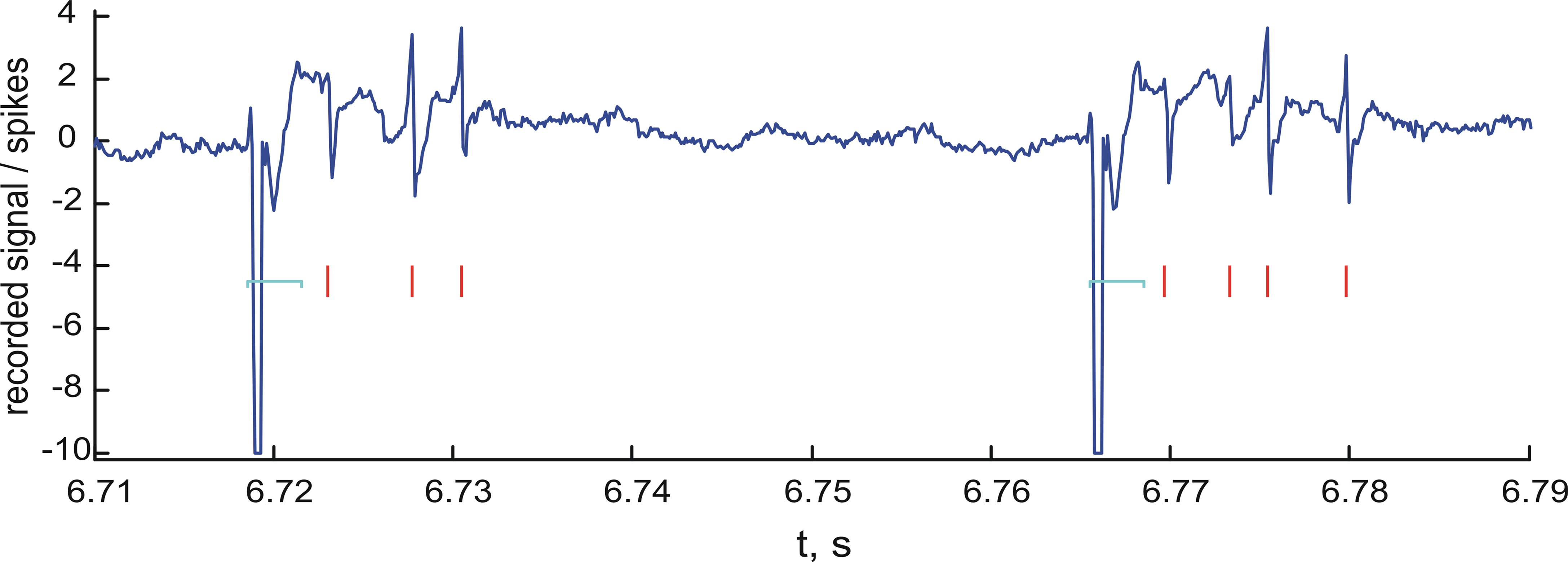
Figure 3. Spike detection. Sample segment of the raw recorded signal (blue line) and the detected spikes (red marks). Units on the vertical axis are mV. Notice the stimulation artifacts in the form of large negative pulses. The artifact cancellation periods are shown by light blue horizontal brackets.
The procedure used for online spike detection during the closed-loop experiments is described in Table 1
. The minimal spike magnitude and the maximal spike duration values used for different experiments session are shown in Table 2
. To avoid confusion between the stimulation artifacts and spikes, the acquired raw signal immediately following each stimulation pulse was discarded. The duration of discarded signal (the artifact cancellation period) was set to 3 ms for all experiments. The spike detection procedure in Table 1
skipped segments of the raw signal during the artifact cancellation periods.
The External Dynamical Systems
We used two different external systems with dynamical dimensions of two and four referred to as the 2D and the 4D system. These systems are real-time simulations of, respectively, a single point-mass and two masses connected by a spring. Both masses move along a line. For both systems, the control signal u determines the external force acting on mass m1, and the position of mass m1 determines the read-out signal y. The point-masses move within a potential force field, and there is a damping element between each point-mass and the ground. These dynamical features were established to induce the combined system to explore a sufficiently wide variety of behaviors. The Supplementary Material provides a detailed description of the two simulated dynamical systems.
The Interfaces
The neural tissue was connected to an EDS, thus forming a closed-loop composite system. The composite system had two signal pathways: (i) a stimulating electrode conveyed the read-out signal of the EDS to the neural tissue; (ii) the signal recorded from the neural tissue determined a control signal for the EDS. The read-out signal, y, of the external system (refer to Eq. 1) was:

The input interface implemented a non-linear mapping from the external system’s read-out signal, y, into the input signal, i (Figure 4
):

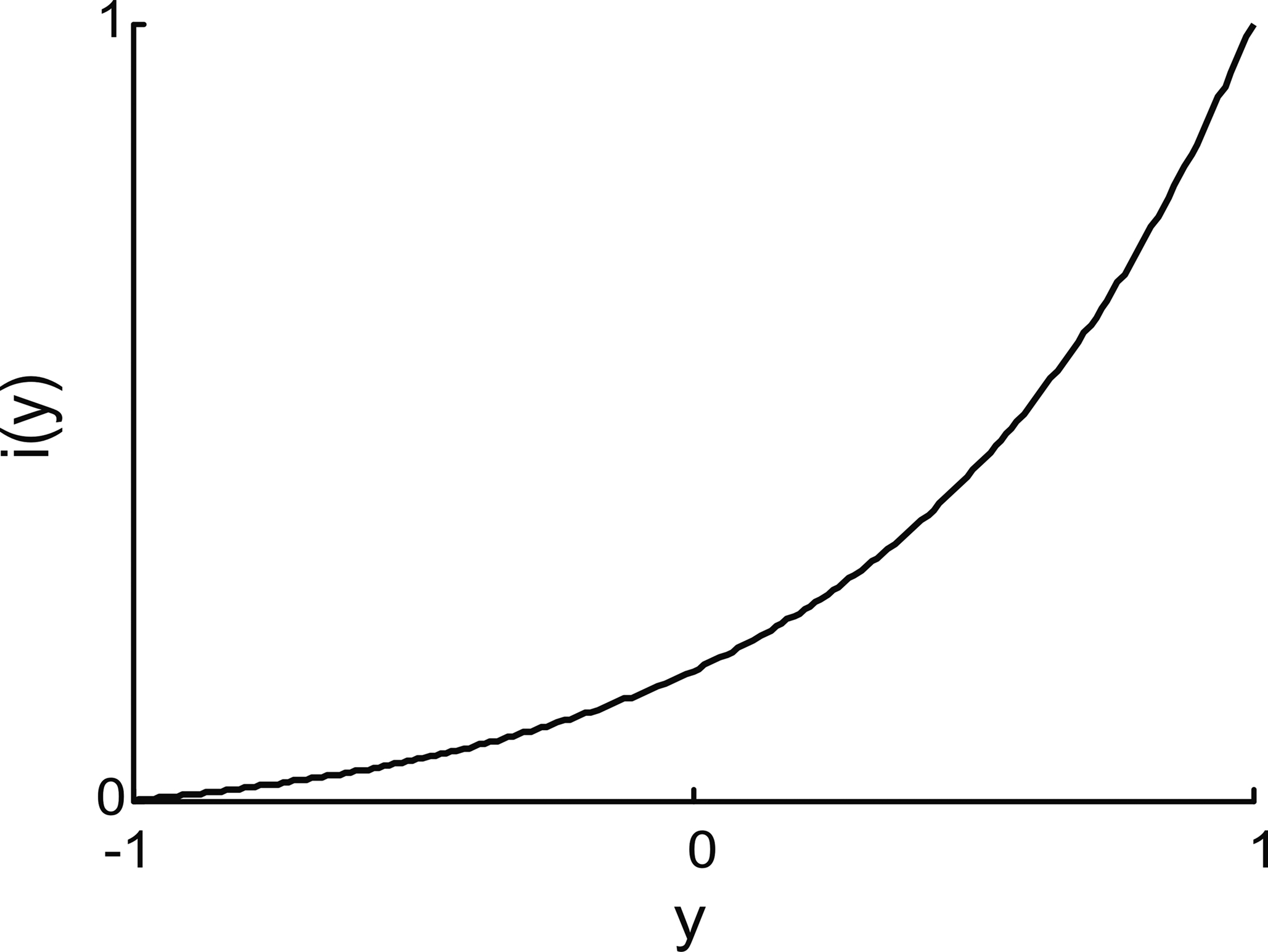
Figure 4. Input interface mapping (Eq. 9). This particular shape of the input interface mapping was chosen to represent the light intensity signal as a function of robot orientation in the experiments that use the same brain–machine interface setup with a mobile robot as the external device (Fleming et al., 2000
).
The position of the simulated point-mass, x1, and hence the read-out signal, y = x1, was constrained to stay within the interval [−1, 1]. Accordingly, the input signal, i, remained within [0, 1]. The “shape” parameter, a, regulated how “curved” was the function (Eq. 9); we used a = 5.This particular form of the input interface mapping was chosen because it is a monotonic and mildly non-linear function. The same expression was used in earlier studies where the neural tissue was connected to a small mobile robot (Fleming et al., 2000
).
The output interface was only used for normalization purposes. Different neural preparations provide different ranges of population spiking rate. The output interface normalized the spiking rate, so that the maximal observed value was mapped into 1; and converted the output signal, o, into a control signal for the external component, u, (see Figure 1
):
The bias, B, and the gain, C, are set to −0.2 and 10 respectively. The maximal observed output value, omax, was estimated for each experimental session in a set of preliminary runs, which are not used to collect data. Particular values of omax used in the experiments are shown in Table 2
.
The Experimental Protocol
Each experiment consisted of a sequence of episodes, in which the BMI system operated for 20 s.
The two external systems were used in alternating episodes. A total of 20 episodes were run in each session. For each episode, the initial configuration of the corresponding external system (positions and velocities of the point-masses) was drawn at random. The episodes were interleaved by periods of rest of 40–100 s. We found empirically that periods of this duration were sufficient to insure stable neural responses across the experiment. We assume that different preparations might require different resting periods.
To reconstruct the dynamical dimension of the composite system we used the trajectories of the external device and not the neural activity, because the latter, being a sequence of spike counts in short-time intervals, is quite noisy, bearing the entire dimension assessment impossible. In the described setup, the external device functions as a filter smoothing out the noisy neural behavior. Since we are estimating the dynamical dimension of the entire system, it is reasonable to analyze the external device trajectories instead of applying another, additional filter to the neural activity. We would like to mention in this regard that the musculo-skeletal system in general (not only of Sea Lamprey) functions as a filter that smoothes out noisy neural activity making the entire system feasible and easily controllable. This could be a factor that determines the filtering properties of muscle tissue.
The temporal structure of the closed-loop system implementation is shown schematically in Figure 5
. A data acquisition card sampled continuously the signal from the recording electrode at 10 kHz rate. The rest of the processing took place in a periodic manner; the experiment loop was repeated once every fixed time period, Δt = 50 ms. The CPU of the computer performed the following operations, without interrupting the data acquisition card:
1. Detect spikes from the 10 kHz signal.
2. Estimate spike rate, o by counting the number of spikes in the interval Δt.
3. Compute the output interface mapping, u(o) (Eq. 10).
4. Simulate one time-step of the EDS, i.e. compute (x1, x2, x3, x4)t + Δt = h(xt,  , u) (see Eq. 24 of the Supplementary Material).
, u) (see Eq. 24 of the Supplementary Material).5. Compute the input interface mapping, i(y) (Eq. 9).
6. Draw the binary stimulation signal (BSS) using the input magnitude, i. Drawing the BSS means choosing BSS equal to 0 or 1 according to the target probability defined as follows. The BSS is a binary signal that determines if the pulse is emitted at the current sweep of the loop. When BSS is equal to 1, the pulse is emitted; otherwise, the pulse is not emitted. The probability of emitting a pulse is therefore:

The input signal, i, determined the current target frequency up to the maximal stimulation frequency, fmax, achieved when i = 1. Particular values used in the experiments for fmax are shown in Table 2
.
7. If the drawn BSS is equal to 1, a command is sent to the stimulation hardware to emit one pulse.
When the elapsed time of the current sweep exceeds Δt, a new sweep is started, a new portion of data is loaded from the data acquisition card, and all the steps described above are repeated again.
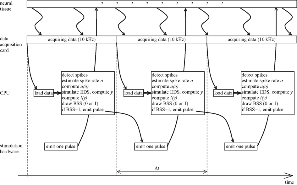
Figure 5. Temporal structure of the experiment. EDS stands for external dynamical system, BSS stands for binary stimulation signal.
Computing the Dynamical Dimension
The state trajectories of an autonomous system do not intersect themselves or each other (Arnold, 1978
). In contrast, the trajectories observed in our experiments exhibit multiple self-intersections. This may be attributed to the fact that they are one-dimensional projections from a higher dimensional state space. To reconstruct the dimension of the composite system, we unfold the observed trajectories into spaces of increasing dimensions and check for the presence of intersections (Kaplan, 1994
). The lowest dimension where the trajectories do not intersect is judged to be the adequate dynamical dimension of the composite system (Abarbanel, 1996
; Kaplan, 1993
). To unfold trajectories into a space of a given dimension d, we used the delayed coordinates space embedding (Mane, 1981
; Takens, 1981
), consisting of d consecutive values of the original trajectory:

where k enumerates the state-points along the embedded state trajectory and τ is the integer lag parameter.
To select a proper lag τ, we employed an approach that uses the first (corresponding to the smallest τ) local minimum of the mutual information between samples (Abarbanel, 1996
), as described in the Supplementary Material. An alternative approach for selecting the lag is to set it equal to the first zero crossing of the autocorrelation of the analyzed signal. However, this only makes sense if the underlying dynamics is linear. The mutual information criterion does not have this limitation, so we used it for the data analysis.
Checking for intersections of the trajectories is a complicated task, which has engendered some controversy (Ruelle, 1990
). Since the sampled trajectories are sets of measure 0 within the embedding space, one can – in principle – never observe an actual intersection (of course for a digitized signal with limited numerical resolution a probability of observing two overlapping samples is non-zero but negligibly small). In spaces of dimension >2, it is only possible to determine that two trajectory segments are close to each other. Most of the existing methods for dimension reconstruction address this difficulty (Kaplan and Glass, 1992
; Kennel et al., 1992
). We propose to take advantage of a priori knowledge about the external device connected to the neural element to remove some of the uncertainties. We used the “delta-epsilon method” developed by Kaplan (Kaplan, 1994
). For each dimension d, the trajectories were unfolded in d-dimensional space and pairs of consecutive points along the unfolded trajectories were analyzed. For two pairs (vi, vi + 1) and (vj, vj + 1), the distance between the first points of each pair is denoted by δ:

and the distance between the second points of each pair is denoted by ε:

Delta-epsilon combinations with small deltas (approaching the limit δ→0) and large epsilons are interpreted as intersections of the trajectories due to projection from a higher dimensional state space onto a space of insufficient dimension. If small deltas always bear small epsilons, it is interpreted as an indication that δ→0 implies ε→0 that corresponds to the elimination of all intersections of the trajectories. In this case, the corresponding dimension is deemed to be an adequate estimate for the dimension of the state space.
We unfolded the observed trajectories sequentially into progressively higher dimensions using delayed coordinates space embedding (Eq. 12). For each dimension, we computed the delta-epsilon combinations and considered n combinations with the smallest deltas. To assess robustness of the method, we have varied n. To test for trajectory intersections in a given dimension d, we compared the magnitudes:

for different d’s (see upper panels in Figure 8
in Section “Results”). Here, Zn is the set of n delta-epsilon combinations with smallest deltas. As the dimension d increased, the corresponding magnitudes εd decreased almost monotonically until they reached a plateau. This saturation points to the dynamical dimension of the composite system. To determine this transition in different preparations, we normalized εd:
The normalization was set so that for each system  spanned magnitudes between 0 and 1 (see lower panels in Figure 8
in the Section “Results”). The assessed dynamical dimension d* was established by setting a threshold h and determining the first threshold crossing in the function vs. d:
spanned magnitudes between 0 and 1 (see lower panels in Figure 8
in the Section “Results”). The assessed dynamical dimension d* was established by setting a threshold h and determining the first threshold crossing in the function vs. d:
spanned magnitudes between 0 and 1 (see lower panels in Figure 8
in the Section “Results”). The assessed dynamical dimension d* was established by setting a threshold h and determining the first threshold crossing in the function vs. d:
Surrogate Data Analysis
To address the noise issue in the dimension analysis (see Abarbanel, 1996
for a general discussion), surrogate trajectories were generated using randomized phases. They do not reflect any implicit dependencies and are used as examples of “pure noise.” Any dimension analysis applied to these trajectories should produce the estimated dimension equal to infinity.
To generate the surrogate trajectories, a Fourier image was computed for each original trajectory. This was done after sub-sampling the trajectory with the time lag τ derived from the average mutual information measure as described above. The phases of the Fourier components were then replaced by random numbers drawn uniformly from [−π, π], while the absolute magnitudes of the Fourier components were preserved. The inverse Fourier transform of the new surrogate image was then computed. This served as the surrogate trajectory. Note that a virtually unlimited number of the surrogate trajectories can be computed for each original trajectory, thus making the outcome of the delta-epsilon dimension analysis much more clear.
Robustness Analysis
As it is common in this type of procedure, the outcome depends on arbitrary parameters, such as the threshold, h, and the number of delta-epsilon combinations, n (Eqs 15 and 17). More definite and robust dimension estimates can be obtained by using two alternative external systems interconnected with the same neural preparation. We tested multiple values for h and n. For each preparation, we computed the dimension of the composite system. The corresponding differences between the estimates for the two external systems were computed for all parameter combinations (see Figure 9
in the Section “Results”). The known difference between the external systems’ dimensions (two) was used to eliminate the parameter combinations that produced inconsistent results. Then, the parameter combinations were s elected that produced the most robust estimates, i.e. the largest number of equal entries in the tables.
To assess the dynamical dimension of the composite system, we used the read-out signal yt of the external system. For both the 2D and the 4D external systems, the read-out signal is the position of the first point-mass, y = x1 (see Eq. 8). Trajectories yt collected during the experiments and used for the subsequent analysis are shown in Figure 6
. For each experimentation session, 10 trajectories were obtained with each of the two EDS (the 2D system and the 4D system). The duration of each trajectory was 20 s.
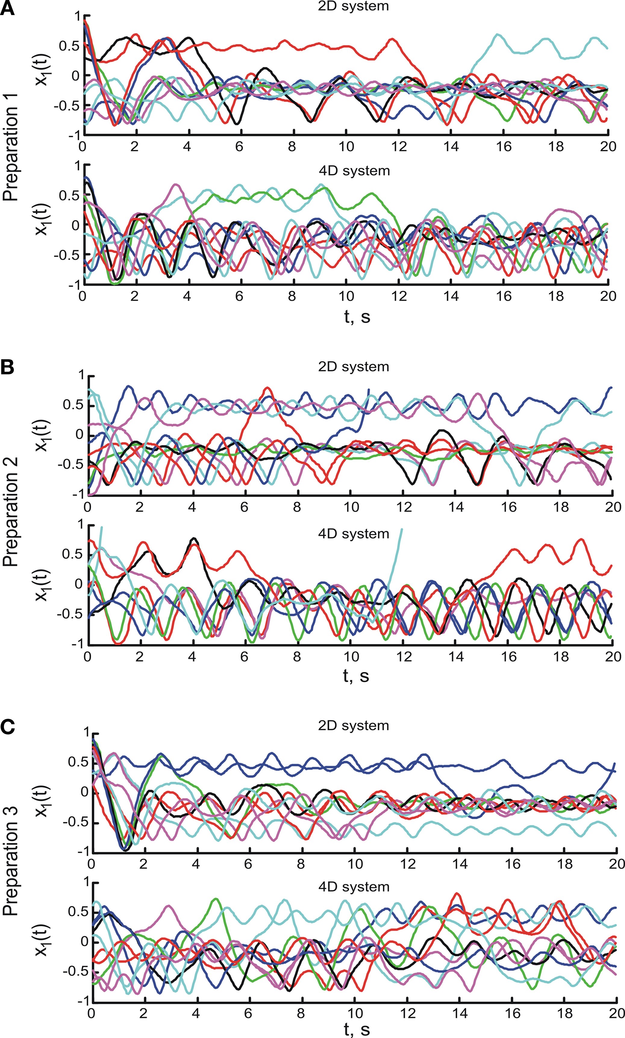
Figure 6. Trajectories of the external dynamical systems obtained during the experiments. (A–C) Show the trajectories for the three preparations respectively. The upper panels show the trajectories obtained using the 2D system, the lower panels show the trajectories obtained using the 4D system. Different colors show different trajectories merely for easier distinction. Note that different trajectories start from different initial positions and velocities.
The dynamical dimension was assessed on the trajectories sampled with lag τ computed individually for each set of trajectories using the mutual information measure described in the Supplementary Material. Each set of trajectories consists of all trajectories collected for one preparation using one particular external system. The average mutual information as a function of the lag τ for the trajectories obtained using three different preparations combined with two alternative EDS is shown in Figure 7
. The smallest τ where the mutual information function reached a local minimum was used as the time lag for the dimension analysis. The corresponding lag is marked as τ0 in each panel in Figure 7
. The lags determined using this method lie between 8 and 10. Lags computed using the first zero crossing of the autocorrelation of the analyzed signal lie between 2 and 4 for most trajectories.
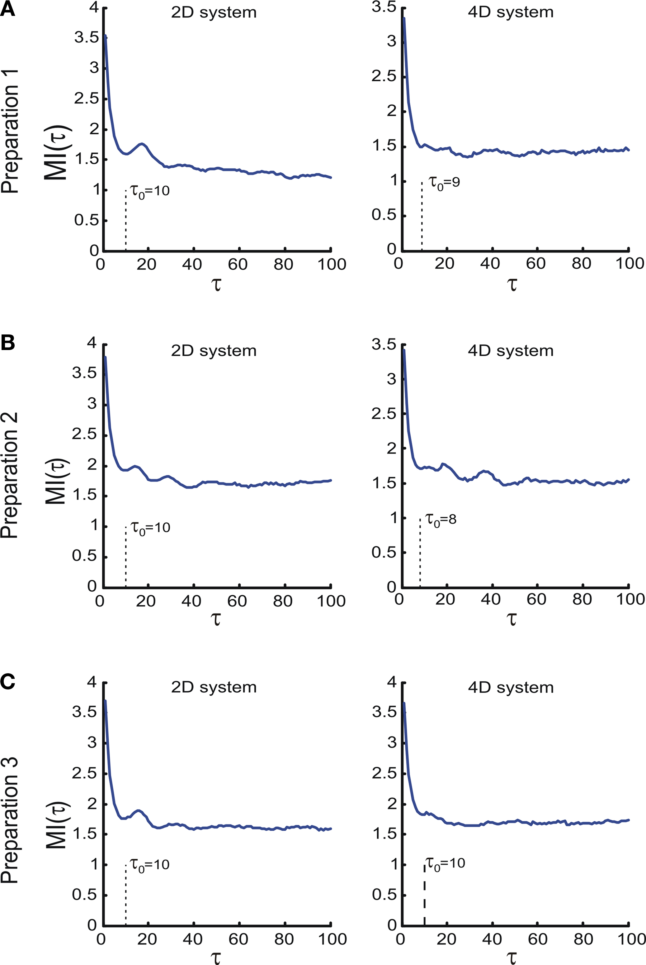
Figure 7. The average mutual information as a function of time lag between points along the observed trajectories. The τ axis units are the steps of the underlying time discretization. (A–C) Show the mutual information for the three preparations respectively. Left panels show the average mutual information computed for the trajectories obtained using the 2D system, rights panels show the data for the 4D system. The time lag, for which the first local minimum of the mutual information is reached, is marked in each panel by τ0.
To assess the dynamical dimension of the composite system, we have computed all delta-epsilon pairs (see Eqs 13 and 14) for each set of trajectories for each dimension from 1 to 20.
To compute the dynamical dimension from the delta-epsilon pairs, we have analyzed εd (Eq. 15) and (Eq. 16) as functions of dimension d. These dependencies are shown in Figure 8
. The two upper panels in Figures 8
A–C show εd (Eq. 15) for different d’s for the two external systems.
(Eq. 16) as functions of dimension d. These dependencies are shown in Figure 8
. The two upper panels in Figures 8
A–C show εd (Eq. 15) for different d’s for the two external systems.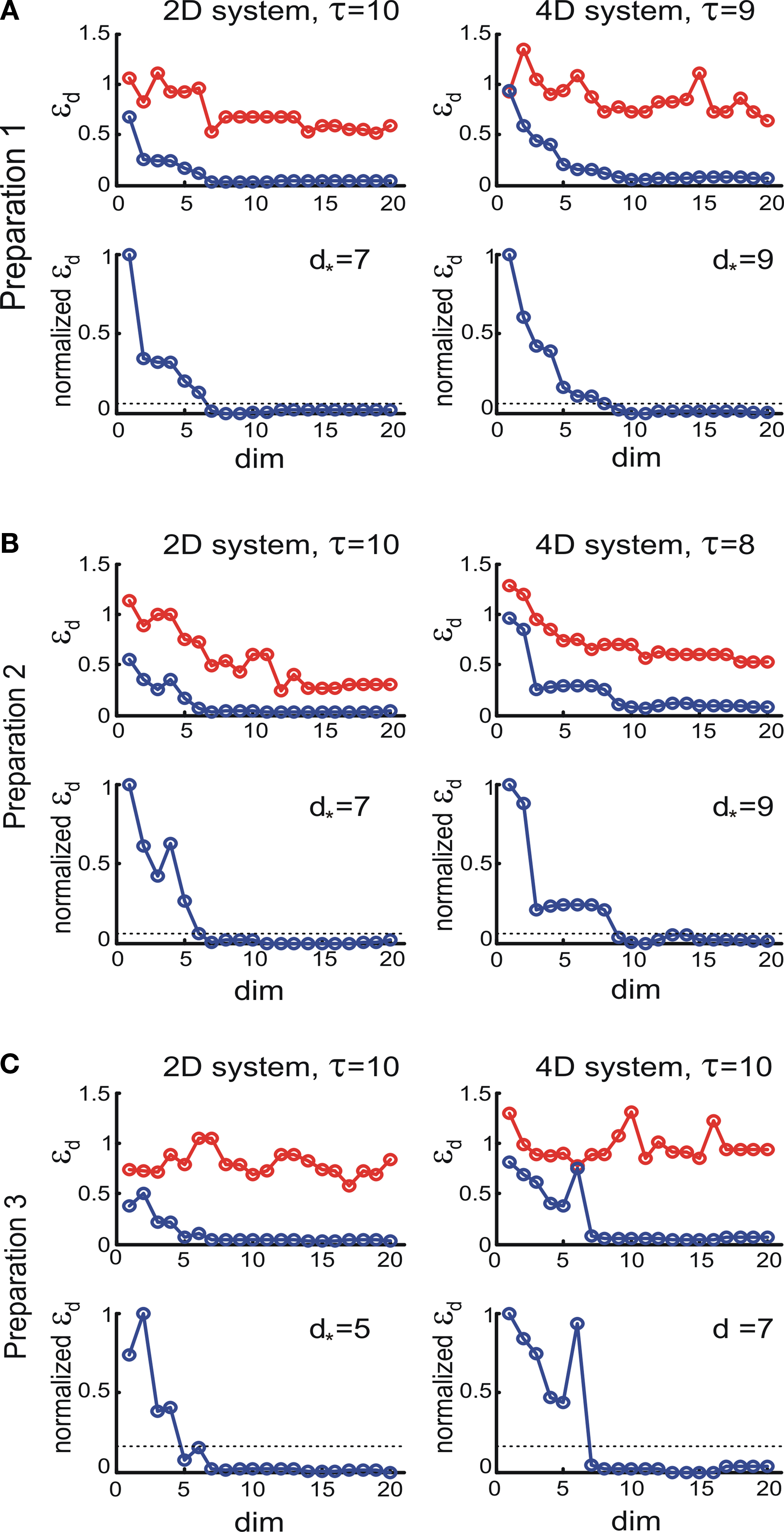
Figure 8 . εd and as a function of d (Eqs 15 and 16). For each preparation, the left panels show the data collected using the 2D external dynamical system, the right panels show the data collected using the 4D external dynamical system. The red plot in the upper panels show εd computed for surrogate trajectories obtained by randomizing phases of the original trajectories. The dotted line in the lower panels shows the threshold h used to assess the dynamical dimension d*.
as a function of d (Eqs 15 and 16). For each preparation, the left panels show the data collected using the 2D external dynamical system, the right panels show the data collected using the 4D external dynamical system. The red plot in the upper panels show εd computed for surrogate trajectories obtained by randomizing phases of the original trajectories. The dotted line in the lower panels shows the threshold h used to assess the dynamical dimension d*.To address the noise issue in the dimension analysis, we have computed a surrogate trajectory for each original one. The results of the delta-epsilon analysis on the surrogate trajectories are shown in Figure 8
by red plots in upper panels in A, B, and C. These plots stand in perfect agreement with the assumption that noise has infinite dynamical dimension. They serve as a good baseline to compare the εd plots of the original trajectories to judge their decay and saturation.
The two lower panels in Figures 8
A–C show the normalized version of εd, (Eq. 16), for different d’s for the two external systems. For each preparation and for any EDS, spans the interval between 0 and 1. The dotted line in each lower panel in Figures 8
A–C shows the threshold level, h, used to compute the dynamical dimension d* (Eq. 17). The latter is marked in each of the lower panels in Figures 8
A–C as well.
(Eq. 16), for different d’s for the two external systems. For each preparation and for any EDS, spans the interval between 0 and 1. The dotted line in each lower panel in Figures 8
A–C shows the threshold level, h, used to compute the dynamical dimension d* (Eq. 17). The latter is marked in each of the lower panels in Figures 8
A–C as well.As mentioned above in Section “Materials and Methods,” we must address the arbitrariness in the parameter choice, which might affect the results; in particular, the threshold, h, and the number of delta-epsilon combinations, n (Eqs 15 and 17). The results of the robustness analysis with respect to the parameters in question are shown in Figure 9
. The dynamical dimension for each preparation was assessed using two factors. First, the consistency between the results for the 2D and the 4D external systems (Figures 9
A–C, left and the middle panels), which requires that the difference between the corresponding entries should be equal to 2. And, second, the general robustness with respect to parameters’ values (Figures 9
A–C, right panels), i.e. the largest number of equal entries in the tables (refer to Section “Robustness Analysis”). The results of this procedure are reported in the last line of Table 2
. The robustness analysis shows that (i) the dynamical dimension assessment is only mildly affected by parameter selection, and that (ii) there are large areas of parameters combinations where the assessments using the two different external systems are mutually consistent.
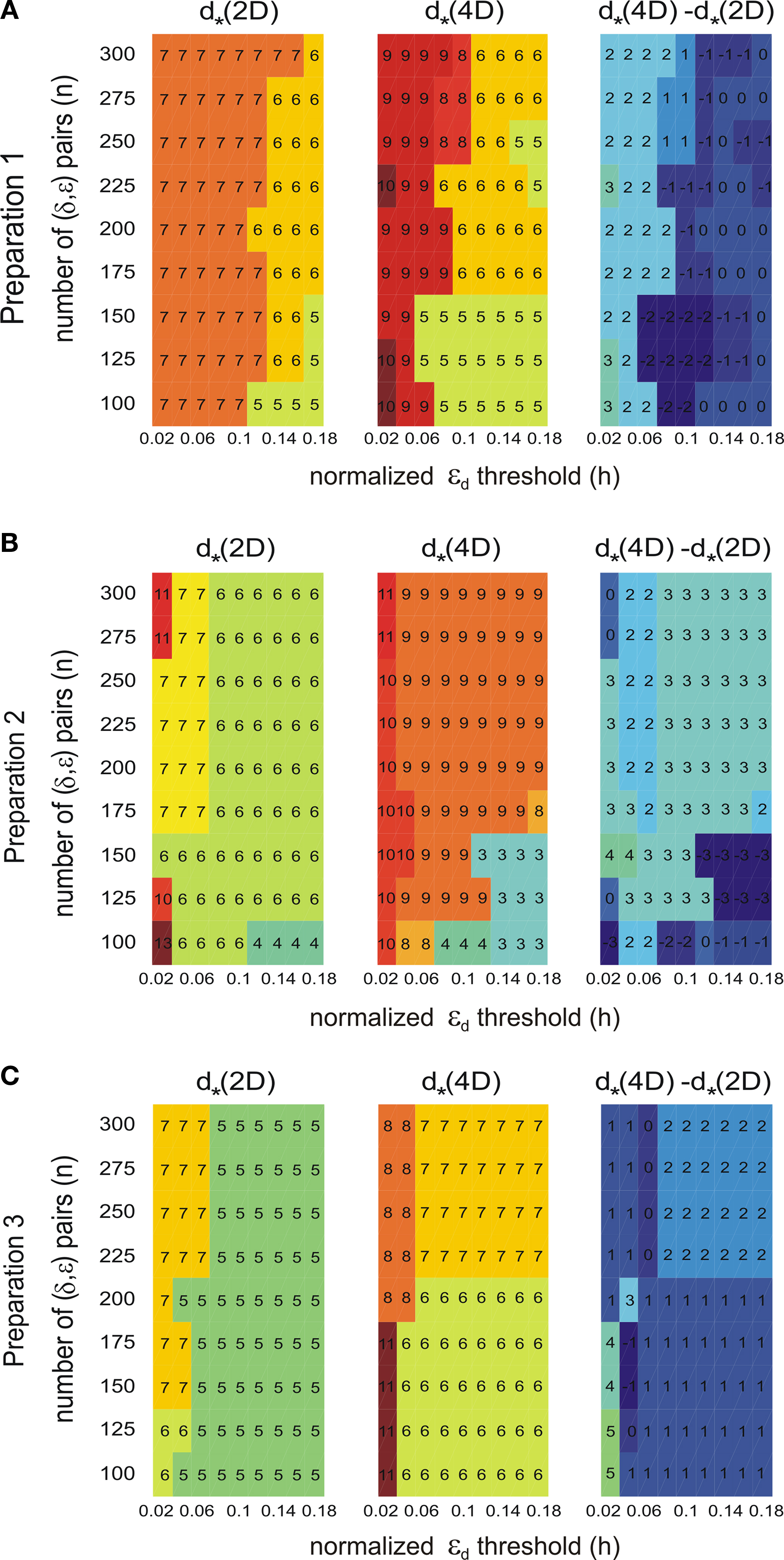
Figure 9. Robustness analysis for the assessed dynamical dimension. In each panel, the columns correspond to different magnitudes of the threshold h (Eq. 17), and the rows correspond to different magnitudes of n (Eq. 15). The three panels in the left column show the assessed dimension, d*, for the data collected using the 2D external system. The three panels in the middle column show the assessed dimension for the data collected using the 4D external system. The three panels in the right column show the difference between the two assessments for each parameter combination. The three panels in each row show the results for a particular preparation, as marked on the left.
To investigate stability of the assessed dynamical dimension over time, we have conducted two additional experimental sessions with one of the preparations (preparation 3). These additional sessions took place after a significant time delay following the first session (see details in Table 2
). Figure 10
shows εd and (Eqs 15 and 16) as functions of d for all three sessions conducted using preparation 3. Figure 11
shows the results of the robustness analysis with respect to the parameters n and h (Eqs 15 and 17) for all three sessions conducted using preparation 3. Figures 10 and 11
use the same representations as Figures 8 and 9
respectively. Note that Figure 10
A shows the same data as Figure 8
C: data from preparation 3 session 1. The same is true regarding Figures 11
A and 9
C. The results of all these assessments are summarized in Table 2
. The dynamical dimensions estimated from the three sessions are the same. This type of analysis is needed to insure (i) that the dynamical dimension is a fixed and well-defined property of a particular preparation, and (ii) that the dynamical dimension is not altered by the process used to assess it. These statements refer to long-time changes that take place (or rather do not take place) in the order of magnitude of hours; this is typical duration of one experimental session for the dynamical dimension assessment. Short-time changes caused by the probing itself cannot be detected by this technique and they might or might not alter the assessed dynamical dimension.
(Eqs 15 and 16) as functions of d for all three sessions conducted using preparation 3. Figure 11
shows the results of the robustness analysis with respect to the parameters n and h (Eqs 15 and 17) for all three sessions conducted using preparation 3. Figures 10 and 11
use the same representations as Figures 8 and 9
respectively. Note that Figure 10
A shows the same data as Figure 8
C: data from preparation 3 session 1. The same is true regarding Figures 11
A and 9
C. The results of all these assessments are summarized in Table 2
. The dynamical dimensions estimated from the three sessions are the same. This type of analysis is needed to insure (i) that the dynamical dimension is a fixed and well-defined property of a particular preparation, and (ii) that the dynamical dimension is not altered by the process used to assess it. These statements refer to long-time changes that take place (or rather do not take place) in the order of magnitude of hours; this is typical duration of one experimental session for the dynamical dimension assessment. Short-time changes caused by the probing itself cannot be detected by this technique and they might or might not alter the assessed dynamical dimension.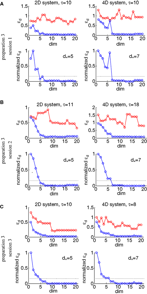
Figure 10. εd and as a function of d (Eqs 15 and 16) for three sessions using preparation 3. See explanations in caption to Figure 8
.
as a function of d (Eqs 15 and 16) for three sessions using preparation 3. See explanations in caption to Figure 8
.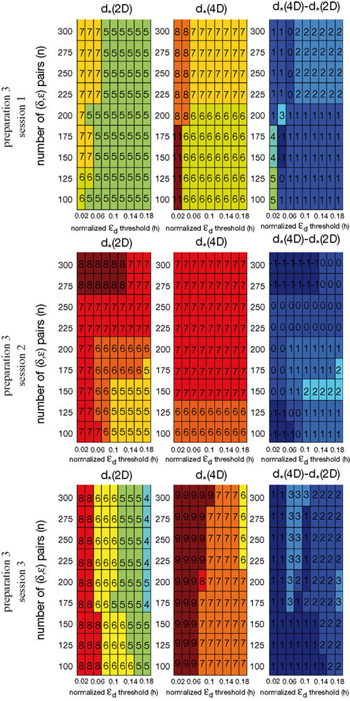
Figure 11. Robustness analysis for three sessions using preparation 3. See explanations in caption to Figure 9
.
This paper describes a methodology for applying dynamical systems theory to the study of properties of neural tissue. We have demonstrated the feasibility of a method for estimating the dynamical dimension of a neural component in a composite neuro-robotic system. We have tested this approach in vitro, using lamprey’s brain stem interconnected with a dynamical system simulated by a computer. These experiments reveal critical issues and bottlenecks of the proposed methods, as well as their weak points and limitations.
The general paradigm used in this work does not try to reveal the dynamics of the neuronal network that exist independently of the external system. This work presents an approach of how to estimate the neuronal network dynamics in the context of closed-loop interactions.
Our findings depends on several contingent factors, including the neural population under study, the electrode placement and the selected parameter settings, such as magnitude, duration, and frequency range of the stimulation pulses. The neural preparation might involve only one neuronal population projecting monosynaptically onto another. Or, it might include multiple synaptic interactions, taking place between stimulation and recording electrodes. Furthermore, the dynamical properties of the neural preparation may be accounted for by changing concentrations of particular ions or substances at different locations along the axons that were stimulated or recorded from, or by various cellular mechanisms, such as channel and autoreceptor dynamics (Schwartz and Alford, 2000
). One would expect to observe different dynamical properties under these different situations.
A specific conclusion regarding the experimental examples provided here is that the estimated neural dynamics may depend quite critically on the placement of the stimulating and recording electrodes. Small variations in electrode position caused a change in the observed dynamical dimension. This may happen due to any of the above-mentioned factors that affect the observed dynamics. For example, the dynamical dimension of preparations 1 and 2 was estimated to be 5, while the dynamical dimension of preparation 3 was estimated to be 3. The dependence of population signals upon the placement of the recording electrodes is a general challenge for BMI systems, and this one is no exception. This is to a large extent an unavoidable problem because the electrode placement – in our case both for stimulation and for recording – defines the biological network under consideration. Nevertheless, once a stable electrode placement has been attained in a BMI system, we can envision the use of this or similar techniques for determining the dynamical properties of the neural tissue that is assigned the control of an external device. While at this time this study has a limited value, we expect that the probing of neural behavior through the interaction with dynamical modules with specific properties – such as damping, inertia, bandwidth, etc.-will provide neural engineers with a simple way for fine tuning the properties of the interface based on solid and easily implementable engineering principles.
The methodology presented in this paper provides a means for assessing the dynamical dimension based only on signal properties. For its most effective use, it is recommended that it be used in combination with other physiological and anatomical techniques providing insight about the cellular structure and mechanisms that determine the observed dynamics. Here, we refer, for example, to the possibility to probe the dynamical properties of portions of neural tissue – either in vivo or in vitro – in conjunction with the application of pharmacological agents that neural plasticity mediated by nMDA or metabotropic glutamate receptors. This would provide focused information on the effects of pharmacological manipulations on the dynamical properties of biological neural networks.
The field of BMIs has been developing very actively for the last few years (Lebedev and Nicolelis, 2006
; Martinoia et al., 2004
; Novellino et al., 2007
; Serruya et al., 2002
; Taylor et al., 2002
; Wessberg et al., 2000
). The direct interaction between the nervous system and external devices has a broad range of applications. In particular, there is a promising potential to use BMIs for reconnecting with the external world patients suffering from a variety of disabling neurological disorders (Donoghue, 2002
; Hochberg et al., 2006
; Kennedy and Bakay, 1998
; Nicolelis, 2003
). The novel feature of our method is the use of the interface with an external device as a research tool. The external device is used to reveal certain characteristics of the neural preparation. In particular, we used two different external devices alternatively with the same preparation in order to address the arbitrariness in the parameter choice for data analysis. At the same time, the external device affects the behavior of the entire BMI system and implicitly shapes the neural activity of the preparation. Evidently, activity patterns exhibited by the preparation in closed-loop interaction with a particular artificial device may differ from those exhibited in natural conditions. In the described experiments, we do not try to simulate the natural behavior or natural neural dynamics. Therefore, all the measurements and conclusions regarding the neural preparation are strictly valid only within the context of a particular BMI system.
We need to stress that in this initial test of our procedure we have used external devices that filtered out high frequency components of the neural signal, so that the resulting behavior was relatively smooth. This however, needs not to be a constraint in other implementations of this approach. We have decided here to introduce an amount of low-pass filtering, in analogy with the smoothing properties of the musculo-skeletal system together with the spinal circuitry (Partridge, 1966
, 1973
). In the general case, different external systems excite different components of the neural dynamics and thus can be used as investigation tools aimed at different operational conditions. Ultimately, the intrinsic dimension of the neural system is likely to be higher than the estimate by our method. This is not necessarily a disadvantage, as the coupled device can deliberately be designed to filter out frequency components and dynamical behaviors that may be detrimental to the effective control of external devices, such as wheelchairs or robotic arms.
Our results indicate that the neural dynamics are captured by relatively simple descriptive models. Here, one must take into account that we used an extracellular electrode. This is not an implicit constraint of the method, as the same concepts can in principle be applied in combination with intracellular recording. As the task of separating single units from extracellular recordings is based on some arbitrary assumptions, we did not make any attempt to this end. We conclude with three considerations on assessing the dynamical dimension of neural preparations in experimental and theoretical investigations:
1. To design effective computational models of a neural preparation, one must take into consideration its dynamical dimension. The dynamical dimension provides the lower bound for the number of tunable parameters for any adequate model. If the state of the neural preparation has four independent components, as we have assessed using the model-less method presented here, then any model trying to match experimental data for a similar input/output arrangement must use at least four independent parameters.
2. Our findings on dynamical dimension suggest the presence of structural features of the preparation, such as connectivity patterns and dynamical properties of particular channels. These findings suggest further investigations with other means. For example, pharmacological agents are used for altering channel properties (Grillner, 2003
), for blocking selected ion channels (Cangiano et al., 2002
), or for altering properties of multi-synaptic transmission (Schwartz et al., 2005
; Takahashi et al., 2001
). The dynamical dimension assessment can be used in combination with these agents to provide a direct evaluation of their effect on neural dynamics.
The general framework of the present study emphasizes the interdisciplinary approach involving experimental neurobiology, engineering, and dynamical systems theory. In previous works (Celletti and Villa, 1996
; Ivanov et al., 1996
; Lee et al., 2001
; Sarnthein et al., 1998
) the same embedding dimension method, has been used for analyzing the electroencephalogram recorded from the brain of different mammals (e.g. rabbits, rats, and humans), and for comparing the results obtained during different experimental (i.e. physiological and pathological, such as epilepsy) conditions. However, the most typical applications of this embedding method are in the area of breathing (Thayer and Moulden, 1997
) and heart rhythm analysis (Bettermann and Van Leeuwen, 1998
; Yeragani and Radhakrishna, 2003
), where the intent of the researches is to identify changes in the electrocardiography recording that could indicate the occurrence of a heart pathology (i.e. arrhythmias). Although there are similar applications in the area of neural function (Jelles et al., 2008
; Kannathal et al., 2004
; Slutzky et al., 2002
; Stam, 2005
), we are not aware of studies assessing the dynamical dimension in a specific portion of the nervous system.
The authors declare that the research was conducted in the absence of any commercial or financial relationships that could be construed as a potential conflict of interest.
This work was supported by ONR grant N000149910881 and NINDS grant NS048845. Authors would like to thank Amir Karniel, M. Shapiro, J.L. Patton, and L. Rubchinsky for their valuable contribution to this work.
The Supplementary Material for this article can be found online at http://www.frontiersinneuroscience/neurorobotics/paper/10.3389/neuro.12.001.2009