Impact of peanut seeding rate on water-use efficiency and yield

Seeds account for one of the highest costs in peanut production. Moreover, the climate in most of the Southeastern US is predicted to become drier and warmer throughout the growing season. Thus, this paper examines how seeding rates alter ecosystem water-use efficiency (WUE) and yield. Experiments with 31.2, 23.0, and 14.8 seed/m were conducted in irrigated fields in Plains, Georgia, US in 2020, 2021 and 2022. WUE was determined continuously at the field scale throughout the growing seasons using the eddy-covariance method. Results suggest that the impact of seeding rate on WUE is highly dependent on weather conditions. With ‘normal’ weather conditions in 2020, both the WUE expressed as the ratio of the net ecosystem exchange (NEE) of CO₂ to evapotranspiration (ET) (noted as WUE_NEE) and the WUE as the ratio of gross primary productivity (GPP) to ET (WUE_GPP) of 14.8 seed/m generally tended to be larger than those of 31.2 seed/m by 6-17% and 6-13% in all accumulated growing-degree day (aGDD) ranges respectively. In particularly wet 2021, both WUE_NEE and WUE_GPP with 31.2 seed/m were larger than those with 23.0 and 14.8 seed/m. This may be because ET in the high seeding rate was hindered more than those in the lower seeding rates in such wet conditions. In contrast, the hot dry weather conditions early in 2022 season (aGDD 500-1000, the period of beginning bloom – full pod) led to high respiration rates with 14.8 seed/m and thus to much lower NEE values. As a result, WUE_NEE of the low seeding rate was much lower than those of 23.0 and 31.2 seed/m by 65% and 70% during the period respectively, but the WUE_GPP of the low seeding rate was equivalent to those of the higher seeding rates. The mid seeding rate had the greatest yield among seeding rate treatments in the wet season and had yield equivalent to other seeding rates in other two years, making it the best option in this three-yr study. The mid seeding rate is recommended to obtain both high yield and high WUE in a hot dry year and high yield in a rainy year.

1 Introduction

Georgia produces the largest amount of peanuts in the most planted area in the thirteen states growing commercial peanut (Arachis hypogaea L.) in the United States, which ranks the fourth in the world in terms of peanut production after China, India, and Nigeria (www.nationalpeanutboard.org). With 277,210-313,632 ha of peanut planting area, Georgia produced about 52-53% of total peanut production in the USA in 2021-2023 (USDA/NASS, 2024).

Peanut seeds account for the greatest cost beside pesticides in peanut production (Smith and Smith, 2010, 2012; Tubbs et al., 2011). These can contribute up to 20% of the total cost (UGA extension, 2024, https://agecon.uga.edu/extension/budgets.html), particularly for large-seeded cultivars such as Georgia-06G (Branch, 2007; Smith and Smith, 2012; Hagan et al., 2015).

Planting fewer seeds leads to a reduction of plant stands thus reducing the yield. On the other hand, overseeding not only increases the cost, but also leads to increased competition for light, water, and nutrients. This competition leads to weak plant stands while not increasing the yield beyond a certain point (Minton and Csinos, 1986; Wehtje et al., 1994).

Previous research has addressed the influence of seeding rate on various aspects of peanut production:

1. plant characteristics such as plant height (Tewolde et al., 2002; Tubbs et al., 2011; Ekram et al., 2019), number of branches (Tewolde et al., 2002; Ekram et al., 2019), leaf area index (LAI) (Tewolde et al., 2002; Tallarita et al., 2021), and plant dry weight (Tewolde et al., 2002; Tallarita et al., 2021);

2. yield and pod/nut properties such as pod number and weight (Tewolde et al., 2002; Ekram et al., 2019; Bakal et al., 2020), pod and/or kernel yield (Sorensen et al., 2004, 2007; Tubbs et al., 2011; Konlan et al., 2014; Hagan et al., 2015; Morla et al., 2018; Ekram et al., 2019; Bakal et al., 2020; Oakes et al., 2020; Sujathamma and Santhosh Kumar Naik, 2022), protein percentage (Bakal et al., 2020; Tallarita et al., 2021), oil content (Ekram et al., 2019; Bakal et al., 2020; Tallarita et al., 2021), and other compositions (Tallarita et al., 2021);

3. diseases (Wehtje et al., 1994; Black et al., 2001; Branch et al., 2003; Sorensen et al., 2007; Hagan et al., 2015); and

4. economic return (Sorensen et al., 2007; Tubbs et al., 2011; Konlan et al., 2014; Oakes et al., 2020).

Tubbs et al. (2011) experimented with seven cultivars in single and twin row patterns at three seeding rates (17, 20, and 23 seed/m) on a sandy loam soil at Plains, GA. They reported that the 17 seed/m rate in a twin row pattern tended to have lower yields, but its net returns were not diminished compared to the higher seeding rates since lower seed costs offset yield reductions. Among the seven cultivars, Georgia-06G and Florida-07 had the highest yield and adjusted net revenue, while Tifguard and Georgia Green had the lowest overall yields. Hagan et al. (2015) experimented with three cultivars Georgia-06G, Georgia Green, and Florida-07 planted at seeding rates of 6.6, 9.8, 13.1, and 19.7 seed/m in mid-April and mid-May. They found higher yields with 13.1 and 19.7 seed/m than 6.6 seed/m, and higher yields with Georgia-06G and Florida-07 than Georgia Green.

As different seeding rates lead to different plant populations and competition, seeding rates should influence plant photosynthesis and water use and thus water-use efficiency (WUE). This is the hypothesis of the current paper. This aspect has yet to be addressed despite the growing season in the southeastern United States becoming drier: the duration of the dry period throughout the growing season has increased by 130% over the last 120 years (Fill et al., 2019). In addition, a heightened temporal variability in precipitation is reported by NOAA (National Oceanic and Atmospheric Administration) (2021) and IPCC Core Writing Team (2023). These drier conditions call for an increase in irrigated acreage by approximately 2000% from 1976 to 2013 in addition to declining aquifer resources in the Southeast, adding pressure on peanut production (Vörösmarty, 2000; Golladay et al., 2004; Sun, 2013; Williams et al., 2017; Engström et al., 2021). From this, it can easily be seen why documenting the influence of management practices on peanut water use and water conservation is needed to improve sustainable crop production while preserving the highest yield possible.

Water-use efficiency can be defined across various spatiotemporal scales for diverse agroecosystems (Hoover et al., 2023). Ecosystem WUE is defined as the ratio of CO₂ gained through photosynthesis to water lost through evapotranspiration (ET) at the ecosystem level (Baldocchi, 1994). The advanced eddy-covariance (hereafter EC) method has been used successfully to measure CO₂ and water vapor fluxes between the atmosphere and various agricultural, forest, and marine ecosystems (Baldocchi, 1994; Dekker et al., 2016; Anderson et al., 2017; Nahrawi et al., 2020; Wagle et al., 2020; Zhang et al., 2022, 2023; Bogati et al., 2023). Ecosystem WUE can be estimated as the ratio of gross primary productivity (GPP) to ET (Wang et al., 2018), gross ecosystem productivity (GEP) to ET (Law et al., 2002; Niu et al., 2011), or net carbon uptake to ET (Baldocchi, 1994; Scanlon and Albertson, 2004; Niu et al., 2011; Zhang et al., 2022, 2023; Bogati et al., 2023).

As part of a series of peer-review publications characterizing the impact of management practices in peanut production, i.e., planting date (Zhang et al., 2022), planting pattern (Zhang et al., 2023), and tillage practices (Bogati et al., 2023), the present study quantifies the impact of seeding rate on peanut ecosystem WUE using the EC method. Using this method, the WUE is continuously evaluated at the field scale, an improvement to traditional methods with discrete measurements, most often separated in time, and typically using small agronomic-size plots. The study also presents the net CO₂ exchange and ET, in addition to the WUE throughout the growing season. Compared to previous studies by Zhang et al. (2022, 2023) and Bogati et al. (2023) in which only daytime was considered, the current study includes both daytime and nighttime.

2 Materials and methods

2.1 Site description

The three-year study was conducted at the University of Georgia (UGA) Southwest Georgia Research and Education Center (32° 2' 48.912" N 84° 22' 14.3178" W, Figure 1) in Plains, GA, USA in 2020, 2021, and 2022. The soil type of the experimental site was Greenville sandy loam (fine, kaolinitic, thermic Rhodic Kandiudults). Three quasi-flat fields next to each other were selected each year (Figure 1).

Figure 1

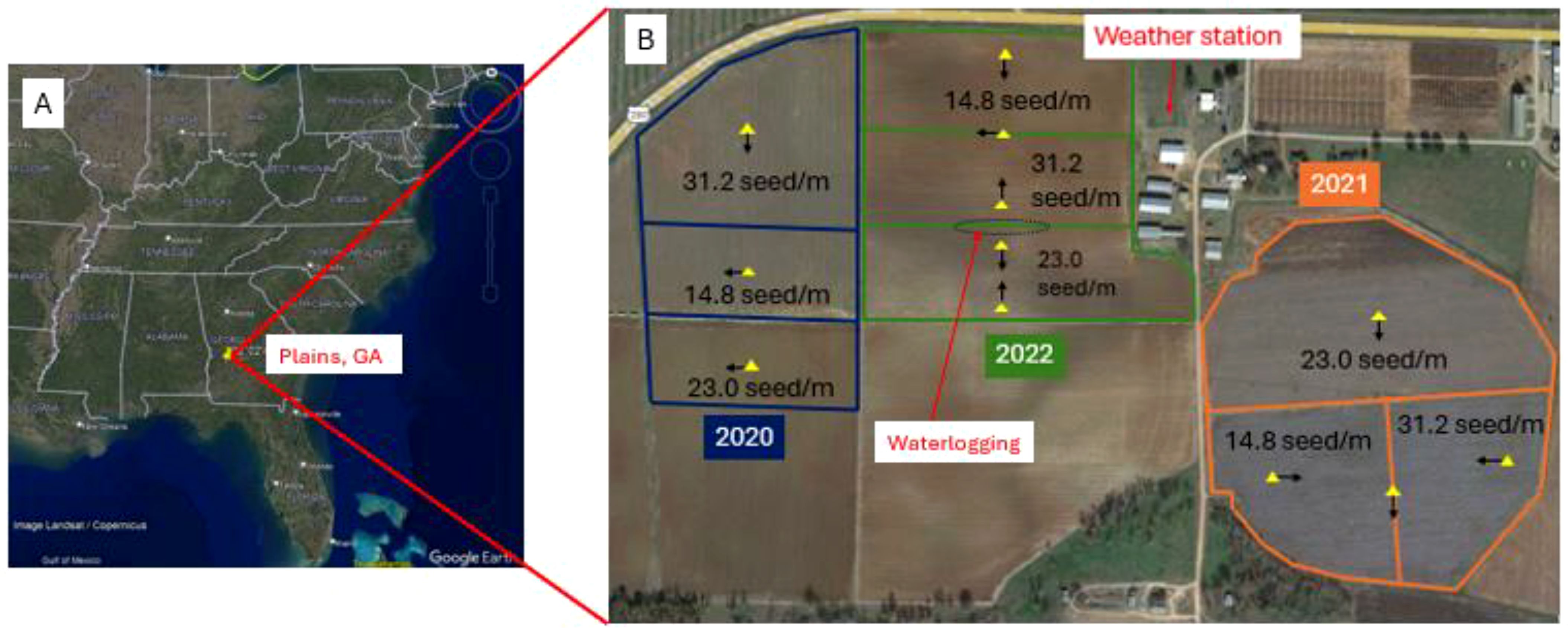
Figure 1. (A) Location of the study site, Southwest Georgia Research and Education Center of the University of Georgia, Plains, GA, USA and (B) fields for seeding rates of 31.2, 23.0, and 14.8 seed/m and locations (yellow triangles) of eddy-covariance systems with the arrows indicating the directions in which the anemometers pointed in 2020-2022.

The planting date was May 15 in 2020, May 17 in 2021, and May 18 in 2022. The large-seeded peanut cultivar Georgia-06G (Branch, 2007) was planted in single row pattern with row space of 91 cm at seeding rates of 14.8, 23.0, and 31.2 seed/m in these fields, respectively. This cultivar was chosen as it is in widespread cultivation in Georgia (Beasley, 2013; Monfort, 2017) because of its high yield potential and resistance to tomato spotted wilt virus (Tubbs et al., 2011). The management practices in the field including irrigation scheduling, fertilization, weed control, and pest and disease spraying were conducted following the guidelines recommended by the University of Georgia Extension (UGA Extension, 2022).

The irrigation was conducted with a pivot irrigation system, with the irrigation drops positioned at 1.8 m above the ground level. The irrigation scheduling was made, based on how long it had been from the prior water event, either in rain or irrigation. Weather forecasts were also used to help guide irrigation decisions. Fertilizer decisions are based on the grid soil sampling conducted by an outside consultant. Fertilizer maps were provided by the consultant and used for grid spread of fertilizers. This was done by using Trimble guidance systems and the Trimble variable rate technology (Trimble Inc., Westminster, CO, USA) installed on a fertilizer buggy. According to grid soil samples, an average of 22.4 kg of P (from diammonium phosphate) per ha was applied in April each year as a pre-plant application.

2.2 Measurements

2.2.1 EC flux measurements

The EC method was used in this study to measure CO₂ and water vapor exchange between the peanut canopy and the atmosphere, i.e., CO₂ flux and ET, respectively. The EC system is composed of an omnidirectional sonic anemometer (CSAT3, Campbell Scientific, Logan, UT, USA) and a fast response open-path CO₂/H₂O gas analyzer (LI-7500, LI-COR Inc., Lincoln, NE, USA) mounted about 1.5 m high from the soil surface on a tripod (Figure 2). The 10 Hz data collected from the instrumentation were logged to a datalogger (CR 1000, Campbell Scientific, Logan, UT, USA). LI-7500 sensors were calibrated and CSAT3 anemometers were checked for the zero offset in the same environmental conditions just before the experiment each year.

Figure 2

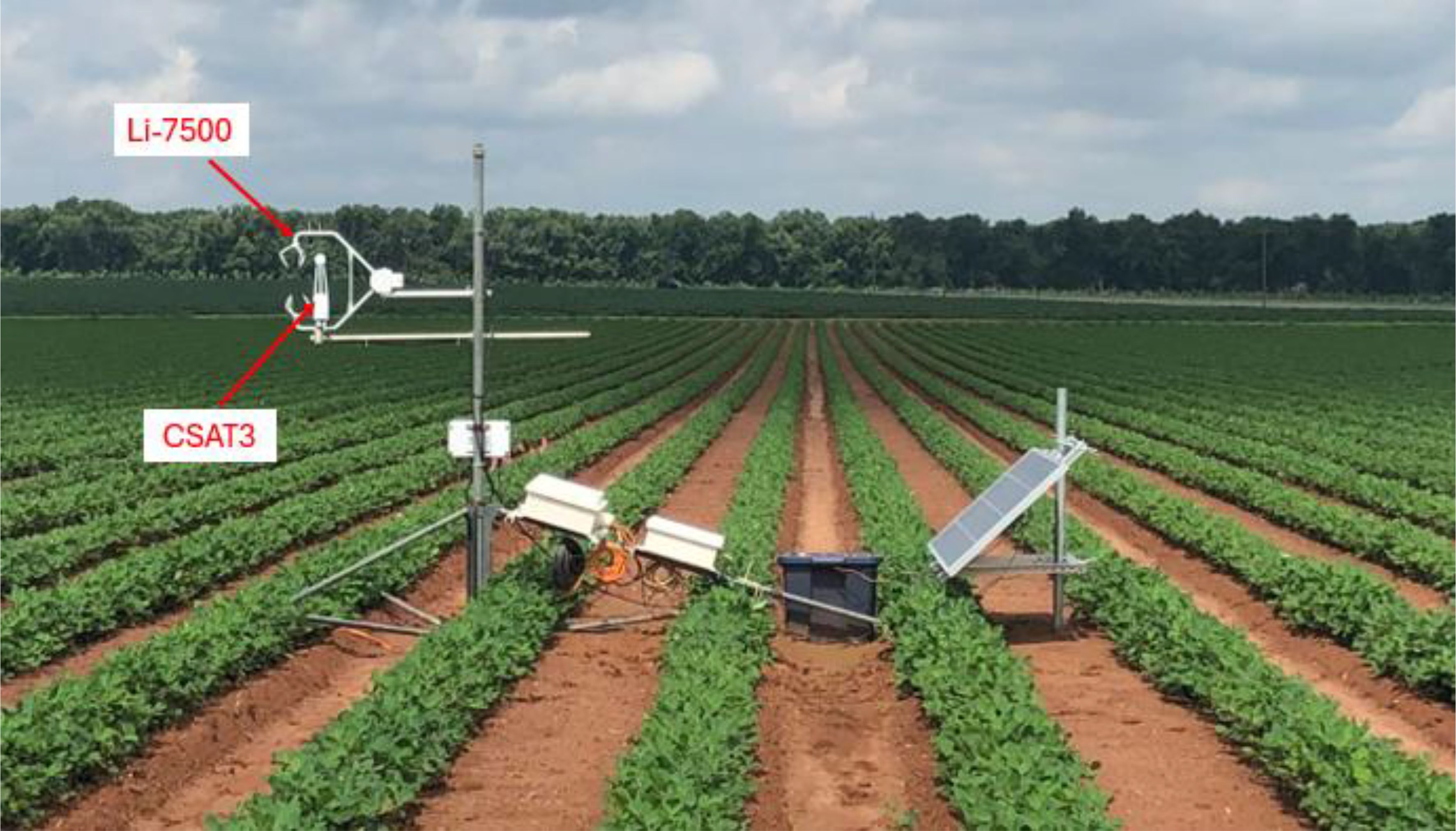
Figure 2. An eddy-covariance system consisting of an omnidirectional sonic anemometer (CSAT3) and the fast-response open-path CO₂/H₂O gas analyzer (LI-7500) installed in a peanut field.

The location of the instrumentation (Figure 1) was chosen to minimize any advection from adjacent fields and to reduce the impact on peanut management practices during the measurement period. EC measurements require that the flux footprint be contained within the field of interest (see Section 2.4 for details of the footprint). In 2020, an EC system was placed approximately in the center of each field with the field area being 6.1, 3.6, and 3.5 ha for the seeding rate treatments of 31.2, 14.8 and 23.0 seed/m from N to S, respectively.

To reduce the data gaps created due to small dimensions of the fields, more EC systems were deployed in 2021 and 2022. In 2021, the field for 23.0 seed/m was large (9.2 ha) and an EC system was set up near the center of the field with the anemometer facing the S direction. The fields for 14.8 and 31.2 seed/m were small, 4.4 and 4.2 ha respectively. Three EC systems were applied: the first EC system was installed on the W side of the field for 14.8 seed/m with the anemometer toward E, the second system on the E side of the field for 31.2 seed/m with the anemometer toward W, and the third system between the contiguous fields for 14.8 and 31.2 seed/m with the sonic anemometer toward S. The collected data were separated for the upwind field according to the wind direction.

In 2022, the field area was 5.1, 4.0, and 4.7 ha for 14.8, 31.2, and 23.0 seed/m from N to S, respectively. The first EC system was set up close to the N side of the northern field for 14.8 seed/m with the anemometer toward S, rejecting data with upwind from NW, N, and NE to avoid the influence of vehicles on the road to the N. The second system was placed between the northern and middle fields and the collected data were separated for the upwind field according to the wind direction. An area of water logging was present in the middle between the middle and southern fields (Figure 1). To exclude the influence of the waterlogging area, two systems were used: the third system was set up near both S of the middle field and N of the waterlogging area with an anemometer pointed N with the data collected for the middle field of 31.2 see/m, and the fourth system was set up near both N of the S field and S of the waterlogging area with an anemometer pointed S with the data collected for the S field of 23.0 seed/m. The fifth system was installed near the southern side of the S field with the anemometer toward N.

2.2.2 Meteorological measurements

Meteorological data was obtained at the UGA weather station at the UGA Research and Education Center at Plains (www.weather.uga.edu) in both 15-min intervals and daily intervals. Solar radiation was measured with a pyranometer (CS301, Apogee Instruments, Logan, UT, USA), air temperature and relative humidity with a humidity and temperature transmitter (HMP60, Vaisala, Vantaa, Finland), wind speed and direction with a wind sensor (034B, Met One, Grants Pass, Oregon, USA), and precipitation with a data-logging rain gauge (TB4, Hydrological Services America, Lake Worth, FL, USA). Vapor pressure deficit (the difference between the vapor pressure in the air and the saturated vapor pressure associated with the air temperature at that time) was calculated with the air temperature and relative humidity. The predominant wind direction was westerly during summer and early fall and easterly during spring and late fall.

2.2.3 LAI measurements

Peanut LAI was measured weekly with a plant canopy analyzer (LI-2000, LI-COR Inc., Lincoln, NE, USA). In each plot, LAI was measured at ten locations with an interval of 0.5 m in one row. At each location, one reading above the peanut canopy and four readings at positions located equally between two rows beneath the canopy on the ground were taken to determine the LAI. In the meantime, the peanut plant height and width were also measured.

2.2.4 Yield measurements

Peanuts were inverted with a KMC inverter (Kelley Manufacturing Co., Tifton, GA, USA) at harvest maturity according to the peanut maturity profile (Williams and Drexler, 1981). The plants were left in the field for approximately 7 d to cure before harvesting. Six representative locations in each field were selected randomly to take biomass samples, stand counts, and assess the yield of each field. Each yield sampling location was 12.2 m long and 1.8 m wide and peanuts were picked with a KMC two row peanut picker (Kelley Manufacturing Co., Tifton, GA, USA). The yield was adjusted to 7% moisture.

2.3 Signal processing and flux calculations

The EC data were processed using the LI-COR proprietary software EddyPro (2019). Low-quality data points, i.e., those characterized by abnormal “automatic gain controls” (AGC) values from the gas analyzers and/or by abnormal diagnostic values from the sonic anemometers were removed. The 30-min periods with more than 10% missing data were discarded. Data spikes were detected and removed according to Vickers and Mahrt (1997). The planar-fit method (Wilczak et al., 2001) was applied to the sonic anemometer data to remove sensor tilt errors. Any linear trend was also removed from each 30-min period. Density fluctuation corrections were made following the Webb-Pearman-Leuning method (Webb et al., 1980).

2.4 Fetch and footprint analysis

Due to the field size limitation, the EC systems were placed at the edge of the fields in an effort to maximize the flux footprint contributed by the field of interest. A rigorous footprint analysis (Kormann and Meixner, 2001) was carried out to check if the footprint is within the upwind fetch of the interested field. The fetch was estimated by measuring the distance from the EC system to the upwind edge of the field in a direction interval of 10 degree using Google Earth Pro (2019).

The footprint is defined as the spatial extent of the source area of fluxes measured at the EC system location (Leclerc and Thurtell, 1990; Leclerc and Foken, 2014; McCombs et al., 2019; Helbig et al., 2021). To ensure that the EC system measures both the CO₂ flux and the ET contributed from the peanut field of interest, the footprint model of Kormann and Meixner (2001) was applied. In this model, the contributing distances to the fluxes are calculated using the Equation 1:

$\begin{array}{ll}{f}_x= \frac{1}{\text{Γ}(\mu )}\frac{{\xi }^{\mu }}{x^{(1+\mu )}}{e}^{-\frac{\xi }{x}}& (1)\end{array}$

where $f_x$ is the percentage of the measured fluxes contributed from the source distance x in the upwind direction from the sonic anemometer, ξ=ξ(z) is the flux length scale that depends on the height above the ground z, μ is a dimensionless model constant, and Γ(μ) is the gamma function. This procedure was performed using the EddyPro software. The flux data with $f_x$ equal to or more than 90% were selected for further processing. If the footprint was larger than the fetch and more than 10% of the flux was contributed from sources outside the field of interest, the flux was removed from further data analysis.

2.5 Data filtering

The calculated fluxes during transition time between day and night of two hours in the morning and two hours in the evening were removed from the dataset (Angevine et al., 2020). This is a standard procedure since atmospheric conditions during these periods are non-stationary (Moffat et al., 2007). Data accompanied by rain were also removed. The data were then filtered with (1) the 0-1–2 system by Mauder and Foken (2006) for data quality to remove data with the combined flag = 2; (2) wind coming from the back of the sonic anemometer (within ±15°) due to flow distortion caused the tripod and flux instrumentation structure; (3) friction velocity u_* threshold (0.1 m s^-1) to remove the data with weak turbulence; (4) the atmospheric stability (z-d)/L< 0 in daytime unstable conditions and (z-d)/L > 0 in nighttime stable conditions to remove the daytime data with (z-d)/L > 0 or stable conditions that indicates local advection bringing heat from outside the interested peanut canopy and the nighttime data with (z-d)/L< 0 or unstable conditions, where z is the EC measurement height above the ground, d the zero-plane displacement height taken as 0.67 times the canopy height, and L the Obukhov length defined as $L=-u_{*}^3\overline{{\theta }_v}/kg\overline{w^{\prime }{\theta }_v^{\text{'}}}$, where u_* is the frictional velocity, $\overline{{\theta }_v}$ the mean virtual potential temperature, $\overline{w^{\prime }{\theta }_v^{\text{'}}}$ the covariance between the surface virtual potential temperature and the vertical wind component, k the von Kármán constant taken as 0.41, and g the gravity acceleration taken as 9.81 m s^-2; (5) filtering data with the above-stated footprint analysis: data points that lie outside the footprint (when 10% or more of the measured flux was contributed from outside the field fetch in that wind direction) were removed.

2.6 Gap filling

An R package REddyProc (Reichstein and Moffet, 2015) was used to fill the gaps in the filtered fluxes of CO₂ and water vapor. As presented in Reichstein et al. (2005), marginal distribution sampling (MDS) gap filling algorithm was adopted. This method was reliable on gap-filling with minimum annual sum bias (Moffat et al., 2007; Paharia et al., 2018). This approach integrates the lookup table algorithm outlined by Falge et al. (2001) with the mean diurnal variation technique. The gap filling using the MDS method was done through the built-in function sMDSGapFill in the R package REddyProc (Reichstein and Moffet, 2015).

2.7 Carbon dioxide flux partition

The net ecosystem exchange (NEE) of CO₂ is the result of two major CO₂-related processes of a plant ecosystem: one is the carbon fixation rate through photosynthesis or GPP, and another is ecosystem respiration (R_e) (Reichstein et al., 2005). The partition of NEE into GPP and R_e can provide an insight into which quantity, GPP or R_e, has more influence on NEE at a given time. In this study, NEE was partitioned into R_e and GPP using the nighttime-based flux partitioning algorithm of Reichstein et al. (2005). For nighttime periods (average solar radiation< 20 W m^-2), GPP is assumed to be zero. Thus, NEE is derived with in the Equation 2:

$\begin{array}{ll}NEE=\{\begin{array}{c}{R}_e --- For nighttime periods\\ R_e-GPP --- For daytime periods\end{array}& (2)\end{array}$

The Lloyd and Taylor model (Lloyd and Taylor, 1994) describing the temperature dependence of R_e was applied to estimate R_e in the current study. The respiration model is expressed with the Equation 3:

$\begin{array}{ll}{R}_e = R_{ref}\times e^{E_0(\frac{1}{T_{ref}-T_0} - \frac{1}{T_a-T_0})}& (3)\end{array}$

where, R_e (μmol m^-2 s^-1) is the sum of autotrophic and heterotrophic respiration at air temperature T_a, R_ref is the respiration rate at a reference temperature T_ref (15°C), E₀ (K) is the activation energy or temperature dependency of R_e expressed in temperature scales and T₀ is the base temperature set to -42.02°C as in Lloyd and Taylor (1994).

The model parameters R_ref and E₀ were estimated by regressively fitting the model to the nighttime data of R_e (= NEE) and Ta for overlapping short-term nighttime periods. Then, the model was used to extrapolate R_e values for daytime periods. R_e and GPP were computed for the entire study period.

2.8 Ecosystem WUE calculations and data partitioning

Peanut ecosystem WUE was calculated in two ways in this study, the ratio of NEE to ET and the ratio of GPP to ET both on a daily base (Zhao et al., 2007; Tallec et al., 2013; Baldocchi et al., 2021), i.e. the Equations 4, 5.

$\begin{array}{ll}{\mathit{\text{WUE}}}_{\mathit{\text{NEE}}}=\frac{NEE}{ET}& (4)\end{array}$

and

$\begin{array}{ll}{\mathit{\text{WUE}}}_{\mathit{\text{GPP}}}=\frac{GPP}{ET}& (5)\end{array}$

The data collected in the present study were partitioned into four periods based on accumulated Growing-Degree Days (aGDD) (Table 1) to account for the change in NEE, GPP, ET, and WUE with crop growth. aGDD is defined as a cumulative amount of the Growing Degree Days (GDD) from planting date to the interested date. The Mills’ Growing Degree Day method (Mills, 1964) was taken in the current paper, as it was shown as the best relationship with peanut maturity (Rowland et al., 2006). The Mills’ GDD is defined in the Equation 6:

Table 1

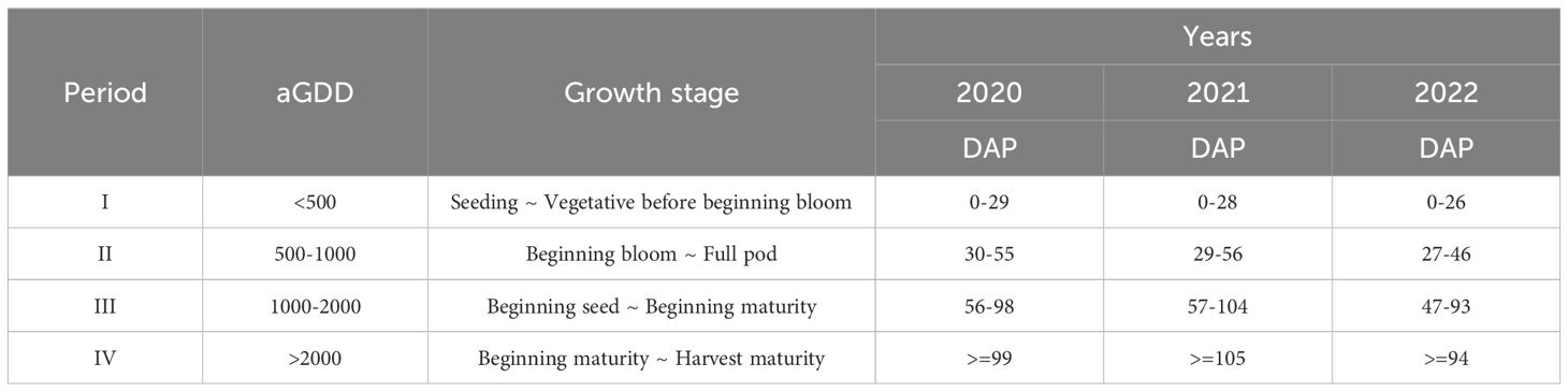
Table 1. The partition of mean 30-min filtered data according to accumulated growing degree days (aGDD) and corresponding days after planting (DAP) and peanut growth stages (Boote et al., 1982).

$\begin{array}{ll}GDD=\frac{ATma{x}_{35}+13.3+ABS[ATmin-13.3]}{2}-13.3+\Delta T_{oc}& (6)\end{array}$

where $ATmax$ is daily maximum air temperature, $ATma{x}_{35}$ is daily maximum air temperature limited to the threshold of 35°C, $ATmin$ is daily minimum air temperature, $\Delta T_{oc}$ is the absolute value of the difference between $ATmax$ and 24.4, and ABS means the absolute function.

2.9 Statistical significance test

The analysis of variance (ANOVA) was performed on ET, Re, NEE, GPP, WUE_NEE, and WUE_GPP using a linear regression model in R (RStudio, 2024). These variables were evaluated as a function of seeding rates, aGDD, and their interactions within each year. Estimated marginal means (least-squares means) were then calculated using the “emmeans” package in R, followed by pairwise comparisons at a significance level of p = 0.1.

Similarly, ANOVA was conducted for weather variables, including average air temperature, average vapor pressure deficit, and total solar radiation, considering their response to year, aGDD, and their interaction. Statistical significance was assessed using the Bonferroni-Sidak test at p = 0.1. Moreover, mean yield across different years was compared at various seeding rates using the least significant difference test at a significance level of 0.1.

3 Results

3.1 Weather conditions

The average daily total solar radiation, air temperature, vapor pressure deficit, total rainfall and total irrigation during various ranges of aGDD < 500, 500-1000, 1000-2000, and > 2000 among 2020, 2021, and 2022 are compared in Figure 3.

Figure 3

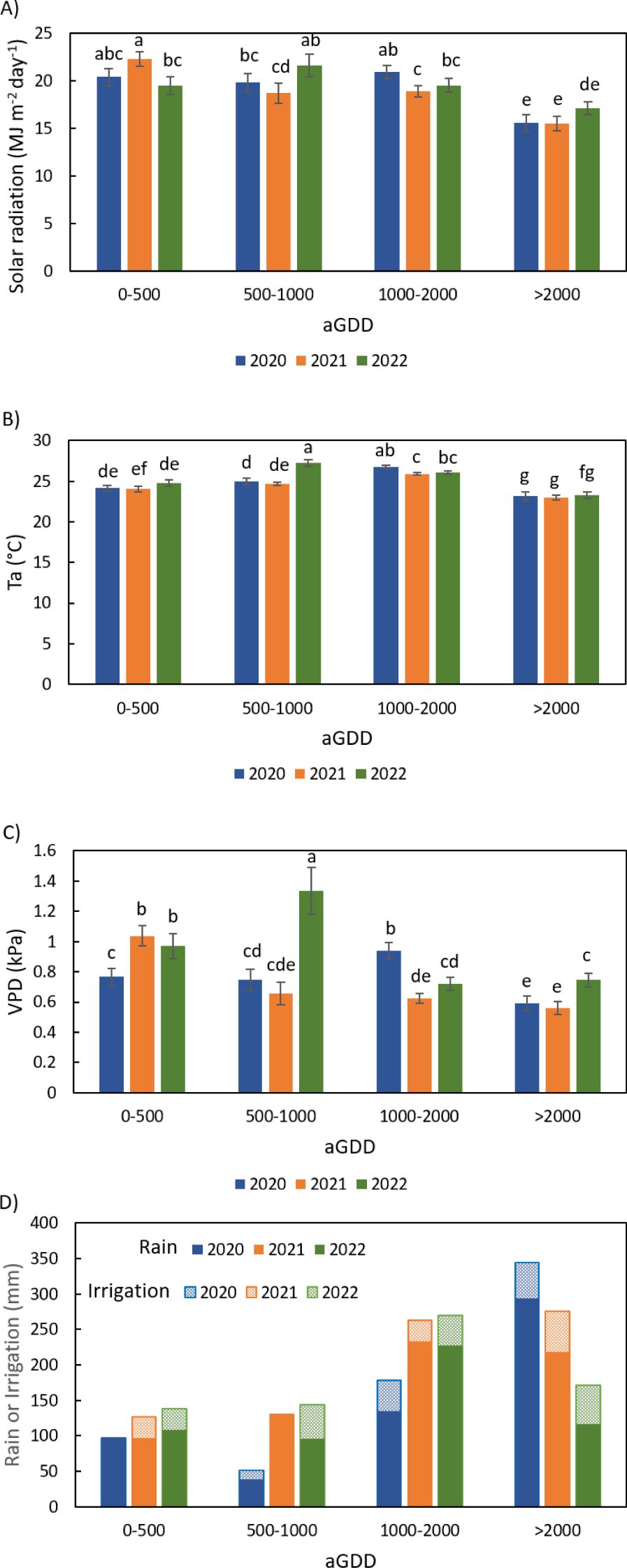
Figure 3. Comparison of weather conditions averaged in various ranges of accumulated growing degree day (aGDD) among 2020, 2021, and 2022: (A) daily total solar radiation, (B) daily average air temperature (Ta), (C) daily average vapor pressure deficit (VPD), and (D) total rainfall and irrigation during the individual aGDD ranges, with error bars indicating the standard error of the mean and letters representing significant test results at the p = 0.1.

The weather conditions varied with both aGDD stage and growing season. The year 2021 experienced lower solar radiation, air temperature and vapor pressure deficit when aGDD > 500 as compared to the 2020 and 2022 growing seasons (Figures 3A-C). This is possibly due to increased cloudiness associated with more rainfall in 2021. The latter was a year characterized by abundant rainfall totaling 676 mm throughout the peanut growing season, i.e. considerably higher than 2020 (564 mm) and 2022 (546 mm) (Figure 3D). Even together with irrigation, the total water supply in 2021 (795 mm) was still the highest, compared to 671 mm in 2020 and 724 mm in 2022. Therefore, 2021 was a wet year in the study period.

On the other hand, the year of 2022 experienced abnormally hot and dry conditions during aGDD 500-1000. The average air temperature was 27.3°C during that period, about 2.5°C higher than both 2020 and 2021 (Figure 3B). The vapor pressure deficit was 1.3 kPa, about double those in 2020 and 2021 (Figure 3C). Solar radiation during the period was also higher than 2020 and 2021 (Figure 3A).

2020 was generally moderate in solar radiation, air temperature, and vapor pressure deficit in the three-yr period (Figures 3A-C). Although the total rainfall in 2020 was also moderate, it was unevenly distributed in the growing season with much less rainfall during aGDD 500–1000 and more rainfall during aGDD > 2000 than in 2021 and 2022 (Figure 3D).

3.2 LAI

Figure 4 describes the LAI of peanut canopies with different seeding rates of 31.2, 23.0, 14.8 seed/m in 2020, 2021, and 2022. In 2020, the 31.2 seed/m peanut canopy had larger LAI than 14.8 seed/m canopy through the growing season, while LAI of 23.0 seed/m was between them (Figure 4A). In 2021, the comparison of LAI with aGDD < 1500 was like that in 2020, but LAI of 14.8 seed/m became larger than those of 23.0 and 31.2 seed/m when aGDD > 2000 (Figure 4B). In 2022, LAI of 23.0 seed/m was the largest among different seeding rates through the growing season, while LAI of 14.8 seed/m was the smallest until aGDD got 2000 and then became similar to LAI of 23.0 seed/m (Figure 4C).

Figure 4

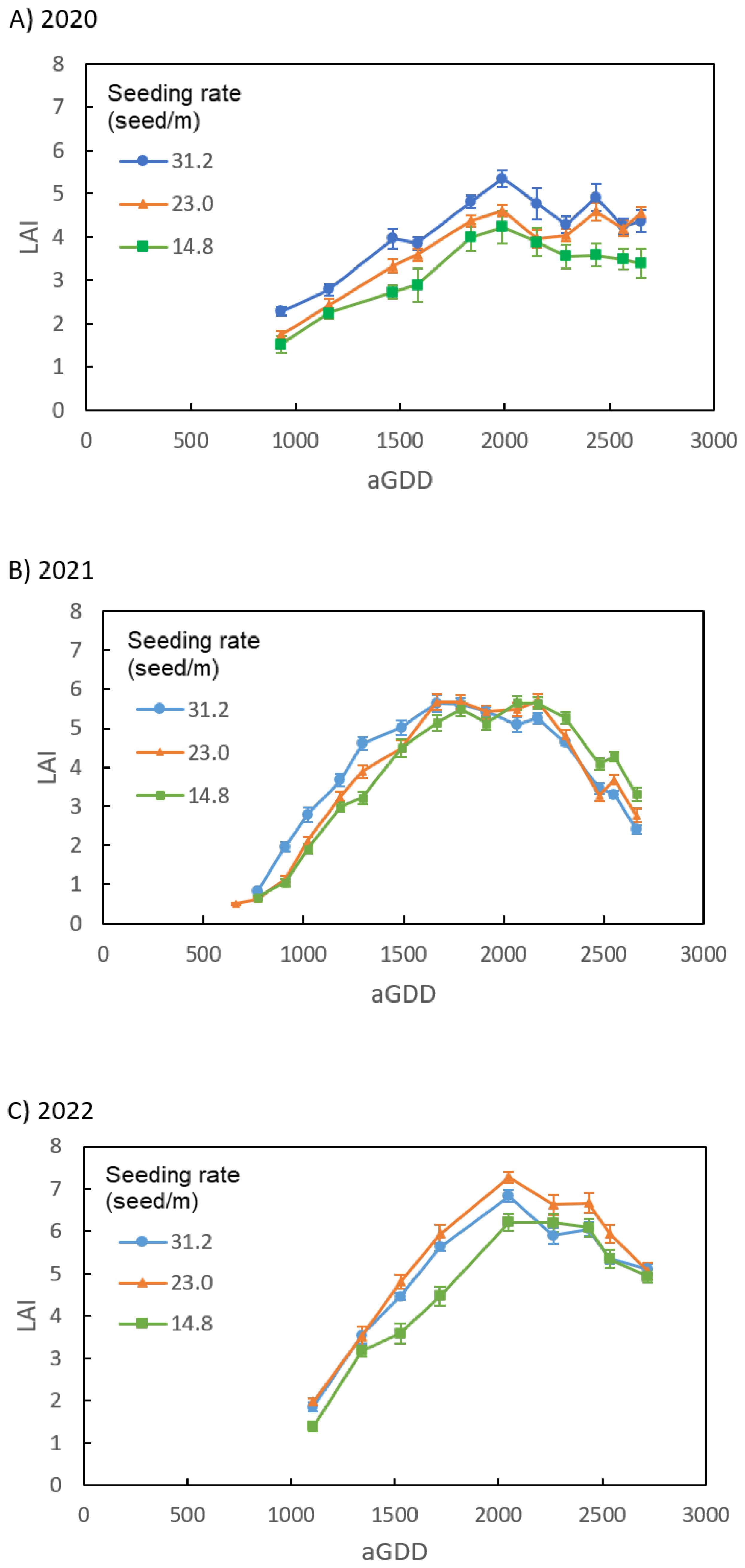
Figure 4. Comparison of the leaf area index (LAI) of peanut canopies among different seeding rates of 31.2, 23.0, and 14.8 seed/m in the growing season of (A) 2020, (B) 2021, and (C) 2022.

3.3 Carbon budget

The averages of daily NEE, GPP and R_e during three ranges of aGDD 500-1000, 1000-2000, and > 2000 in 2020–2022 are compared among the different seeding rates of 31.2, 23.0, 14.8 seed/m in Figures 5–7, respectively. There were no data for 23.0 seed/m in 2020 and aGDD 500–1000 in 2021 due to malfunction of the EC sensors (same for ET and WUE below).

Figure 5

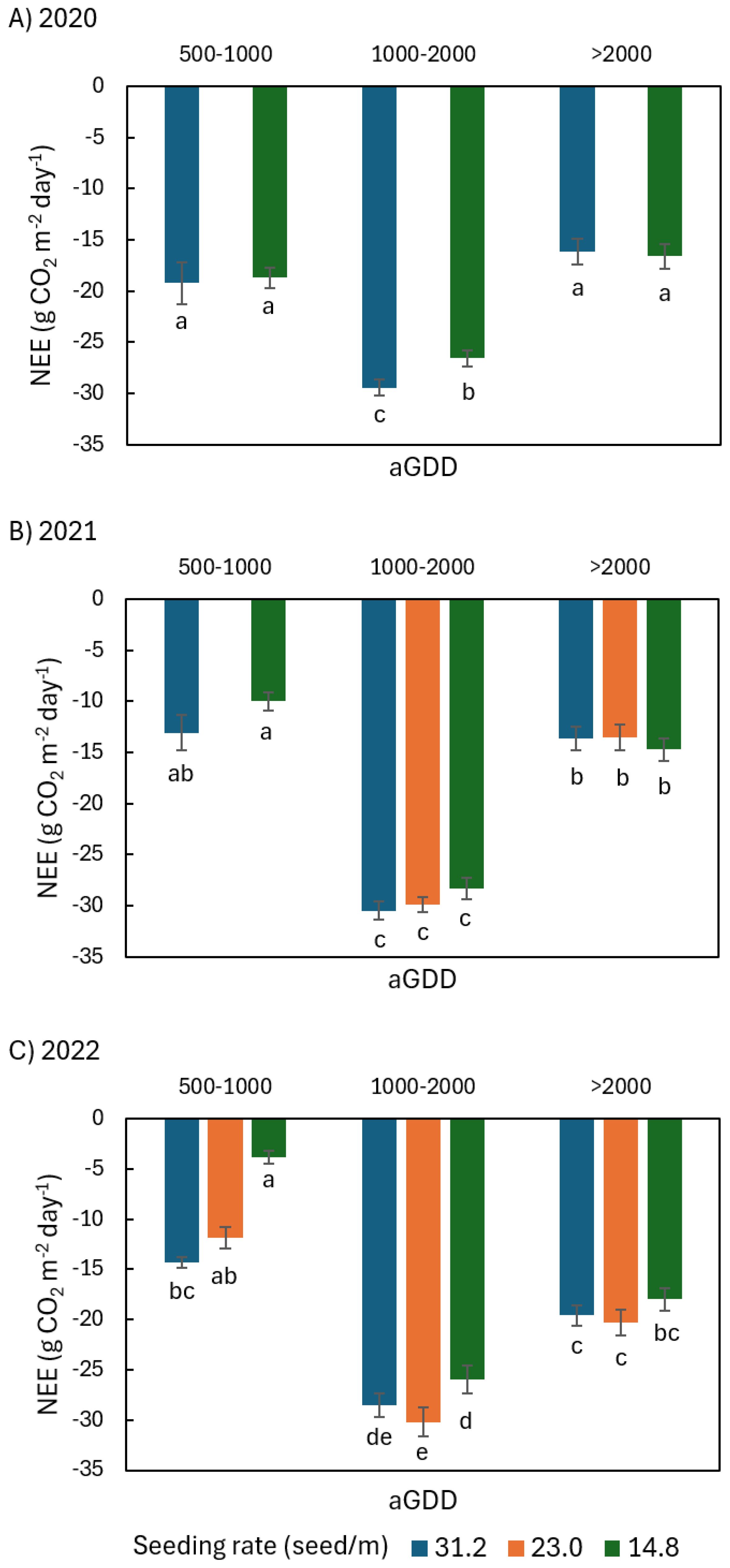
Figure 5. Comparison of the average daily net ecosystem exchange (NEE) of CO2 of peanut canopy among different seeding rates of 31.2, 23.0, and 14.8 seed/m during various ranges of accumulated growing degree day (aGDD) along the growing season in (A) 2020, (B) 2021, and (C) 2022, with error bars indicating the standard error of the mean and letters representing significant test results at the p = 0.1.

Figure 6

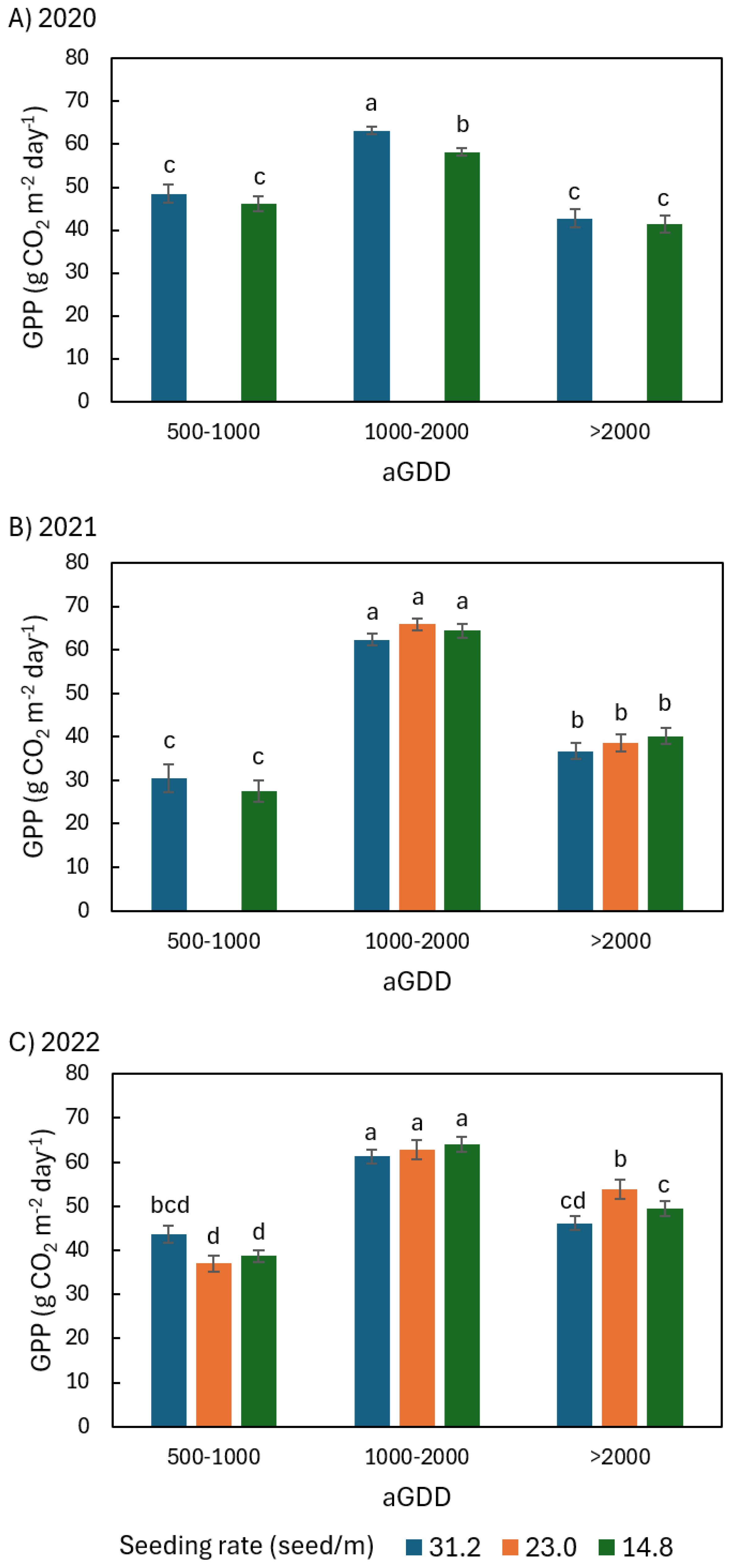
Figure 6. Comparison of the average daily peanut ecosystem gross primary productivity (GPP) among different seeding rates of 31.2, 23.0, and 14.8 seed/m during various ranges of accumulated growing degree day (aGDD) along the growing season in (A) 2020, (B) 2021, and (C) 2022, with error bars indicating the standard error of the mean and letters representing significant test results at the p = 0.1.

Figure 7

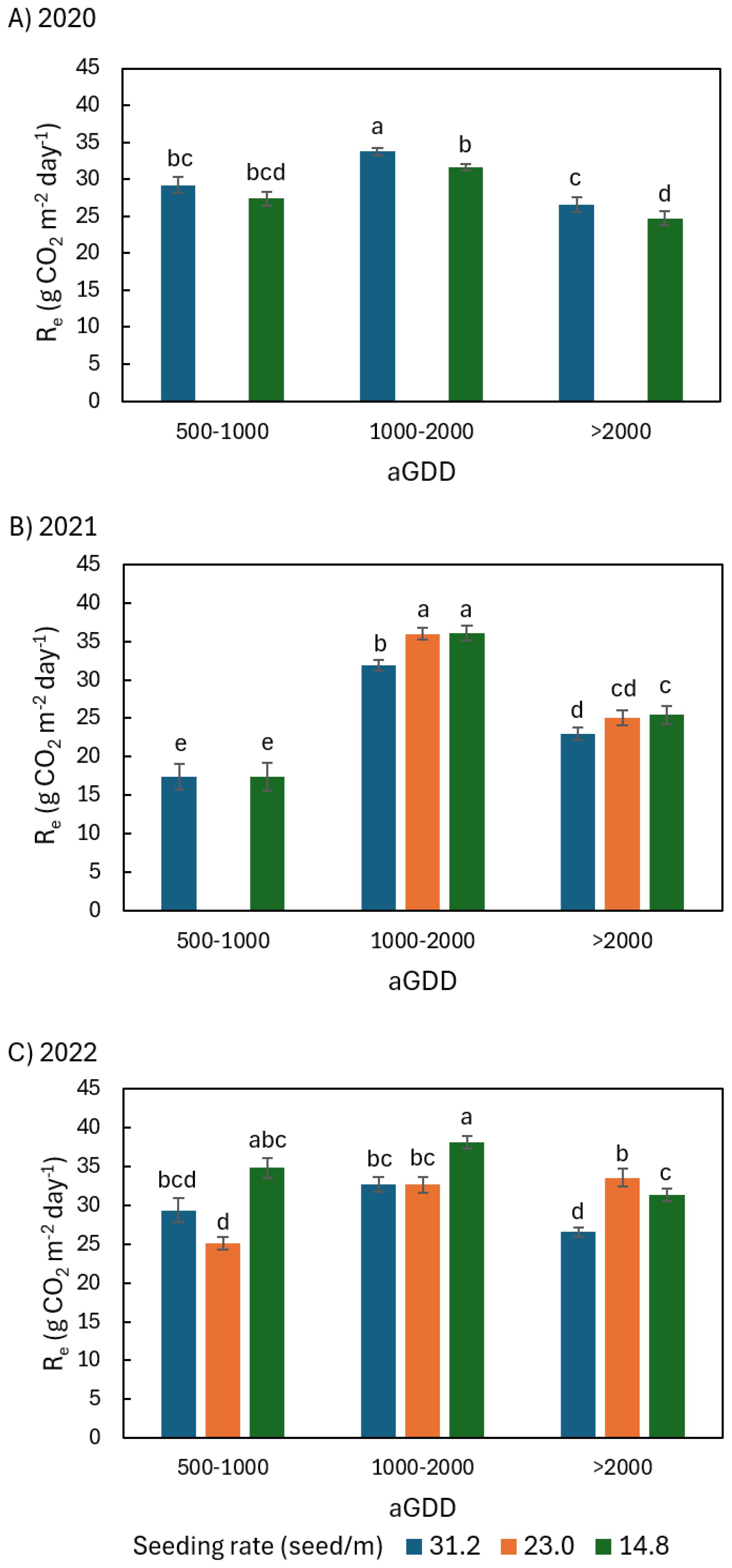
Figure 7. Comparison of the average daily peanut ecosystem respiration (Re) among different seeding rates of 31.2, 23.0, and 14.8 seed/m during various ranges of accumulated growing degree day (aGDD) along the growing season in (A) 2020, (B) 2021, and (C) 2022, with error bars indicating the standard error of the mean and letters representing significant test results at the p = 0.1.

In 2020 during aGDD 1000-2000, NEE_31.2, GPP_31.2, and R_e31.2 (hereafter subscript number denoting seeding rate) were significantly larger than NEE_14.8, GPP_14.8, and R_e14.8 by 2.8, 5.0, and 2.1 g CO₂ m^-2 day^-1, respectively (Figures 5A, 6A, 7A). During aGDD 500–1000 and aGDD > 2000, there was no significant difference in NEE, GPP and R_e between the seeding rates 31.2 and 14.8 see/m, except for R_e31.2 significantly larger than R_e14.8 by 1.8 g CO₂ m^-2 day^-1 during aGDD > 2000.

In 2021, there was no significant difference in NEE and GPP among different seeding rates during each aGDD period (Figures 5B, 6B). But there was a trend that the NEE of 31.2 seed/m was larger than other seeding rates during aGDD 500–1000 and 1000–2000 while the GPP of 31.2 seed/m was smaller than other seeding rates during aGDD 1000–2000 and > 2000. On the other hand, R_e31.2 was significantly smaller than both R_e23.0 and R_e14.8 during periods of aGDD 1000–2000 and > 2000, respectively (Figure 7B).

In 2022, NEE_14.8 during aGDD 500–1000 was only -3.8 g CO₂ m^-2 day^-1, significantly smaller than NEE_31.2 (Figure 5C). The NEE_14.8 values were also significantly lower than NEE_23.0 during aGDD 1000–2000 but not significantly lower than the two other seeding rates during aGDD > 2000. GPP had no significant difference among all three seeding rates during each aGDD period, except for GPP_23.0 significantly larger than both GPP_31.2 and GPP_14.8 during aGDD > 2000 (Figure 6C), although GPP_31.2 tended to the largest during aGDD 500–1000 and the smallest during aGDD 1000-2000. R_e14.8 was either significantly or non-significantly larger than those of other seeding rates during aGDD 500–1000 and 1000-2000 (Figure 7C). During aGDD > 2000, it was significant that R_e23.0 > GPP_14.8 > R_e31.2.

3.4 Evapotranspiration

Figure 8 shows the comparison of daily ET during various ranges of aGDD for the three consecutive growing seasons in 2020-2022, respectively.

Figure 8

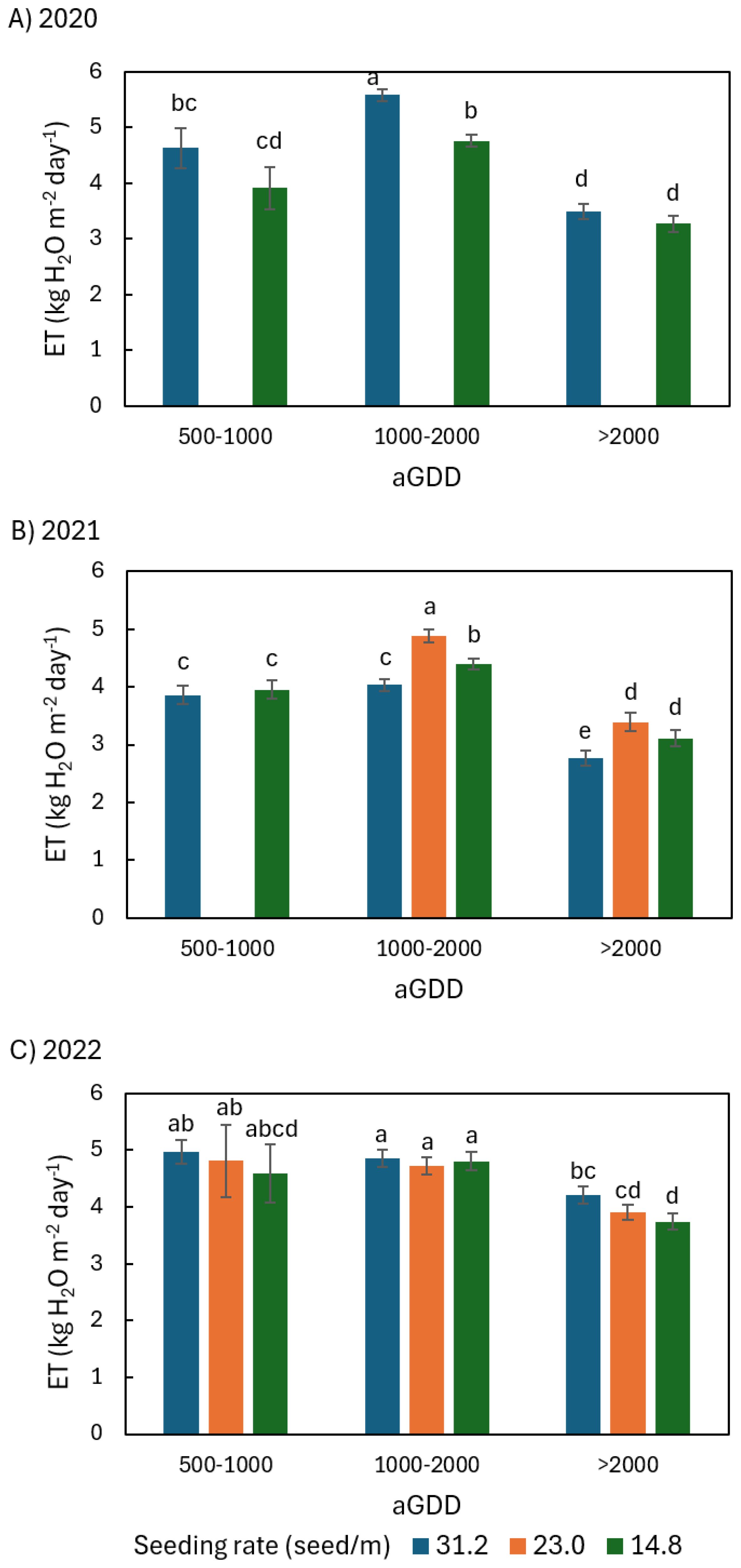
Figure 8. Comparison of the average daily peanut evapotranspiration (ET) among different seeding rates of 31.2, 23.0, and 14.8 seed/m during various ranges of accumulated growing degree day (aGDD) along the growing season in (A) 2020, (B) 2021, and (C) 2022, with error bars indicating the standard error of the mean and letters representing significant test results at the p = 0.1.

In both 2020 and 2022, ET_31.2 generally tended to be larger than ET of other seeding rates during different aGDD ranges (Figures 8A, C). In 2020, ET_31.2 was 4.6, 5.6, and 3.5 kg H₂O m^-2 day^-1 on average during aGDD 500-1000, 1000-2000, and >2000, larger than ET_14.8 by 0.7, 0.8, and 0.2 kg H₂O m^-2 day^-1, respectively, in which only the difference during aGDD 1000–2000 was significant (Figure 8A). In 2022, ET_31.2 > ET_23.0 > ET_14.8 during both aGDD in the range of 500–1000 and aGDD > 2000, while the difference is small among the seeding rates during aGDD 1000-2000. However, only the difference between ET_31.2 and ET_14.8 during aGDD > 2000 was significant (Figure 8C).

In contrast, ET_31.2 tended to be smaller than ET of other seeding rates while ET_23.0 tended to be largest among all seeding rates in 2021 (Figure 8B). During aGDD ranges of 1000–2000 and > 2000, ET_23.0 was 4.9 and 3.4 kg H₂O m^-2 day^-1 respectively, significantly larger than both ET_14.8 and ET_31.2 during aGDD 1000-2000, and significantly larger than ET_31.2 during aGDD > 2000. ET_31.2 was 3.9, 4.0, and 2.8 kg H₂O m^-2 day^-1 in average during aGDD 500-1000, 1000-2000, and >2000, smaller than ET_14.8 by 0.1, 0.4, and 0.3 kg H₂O m^-2 day^-1, respectively.

3.5 Ecosystem WUE

The daily ecosystem WUE was estimated as both ratios of NEE and GPP to ET (Equations 4, 5). A comparison of WUE_NEE between different seeding rates of 31.2, 23.0, and 14.8 seed/m during various aGDD ranges along the growing season in 2020, 2021 and 2022 was plotted in Figure 9. Figure 10 is for the comparison of WUE_GPP.

Figure 9

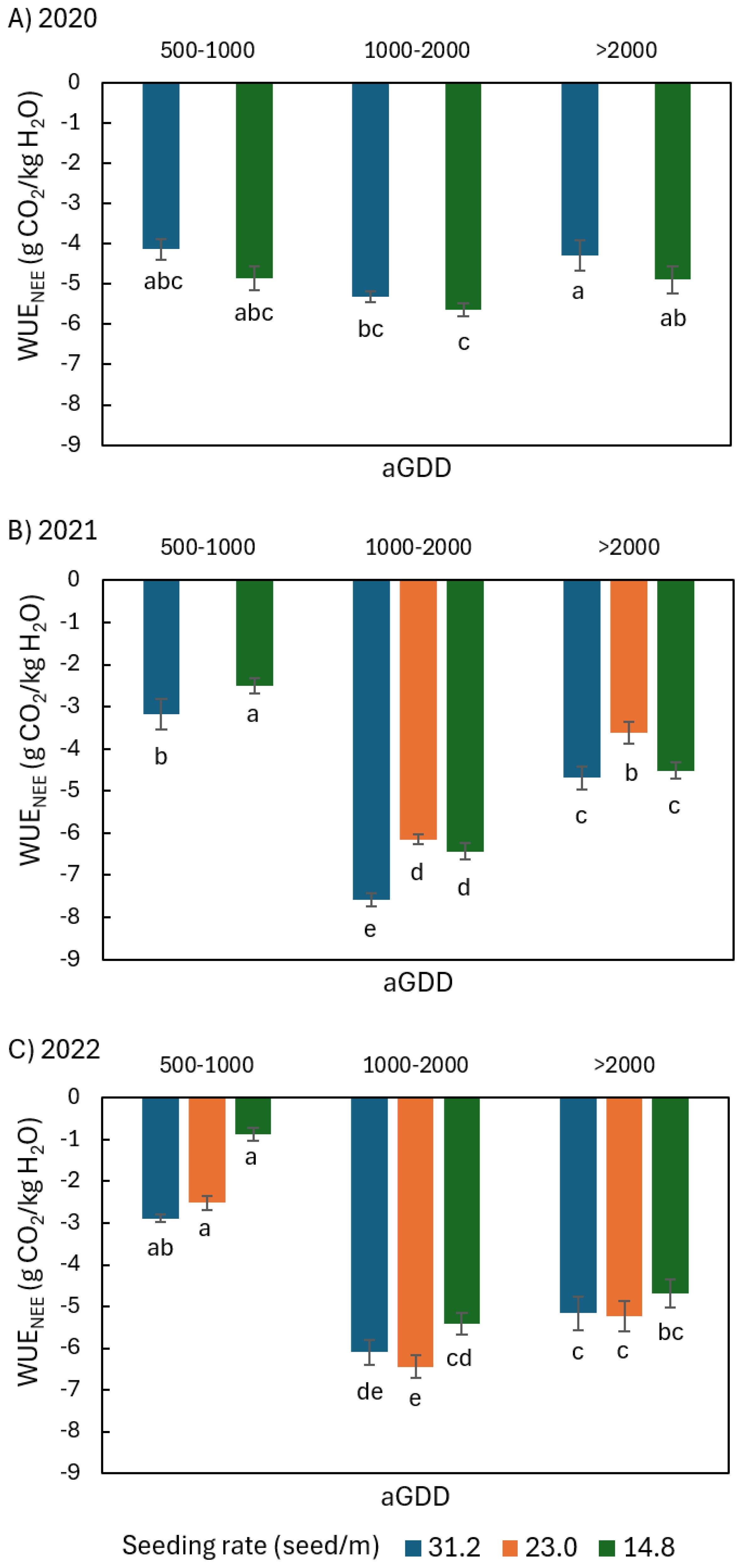
Figure 9. Comparison of the average daily peanut water-use efficiency (WUE) defined as the ratio of daily net ecosystem exchange (NEE) of CO2 to evapotranspiration (ET), noted as WUE_NEE, among different seeding rates of 31.2, 23.0, and 14.8 seed/m during various ranges of accumulated growing degree day (aGDD) along the growing season in (A) 2020, (B) 2021, and (C) 2022, with error bars indicating the standard error of the mean and letters representing significant test results at the p = 0.1.

Figure 10

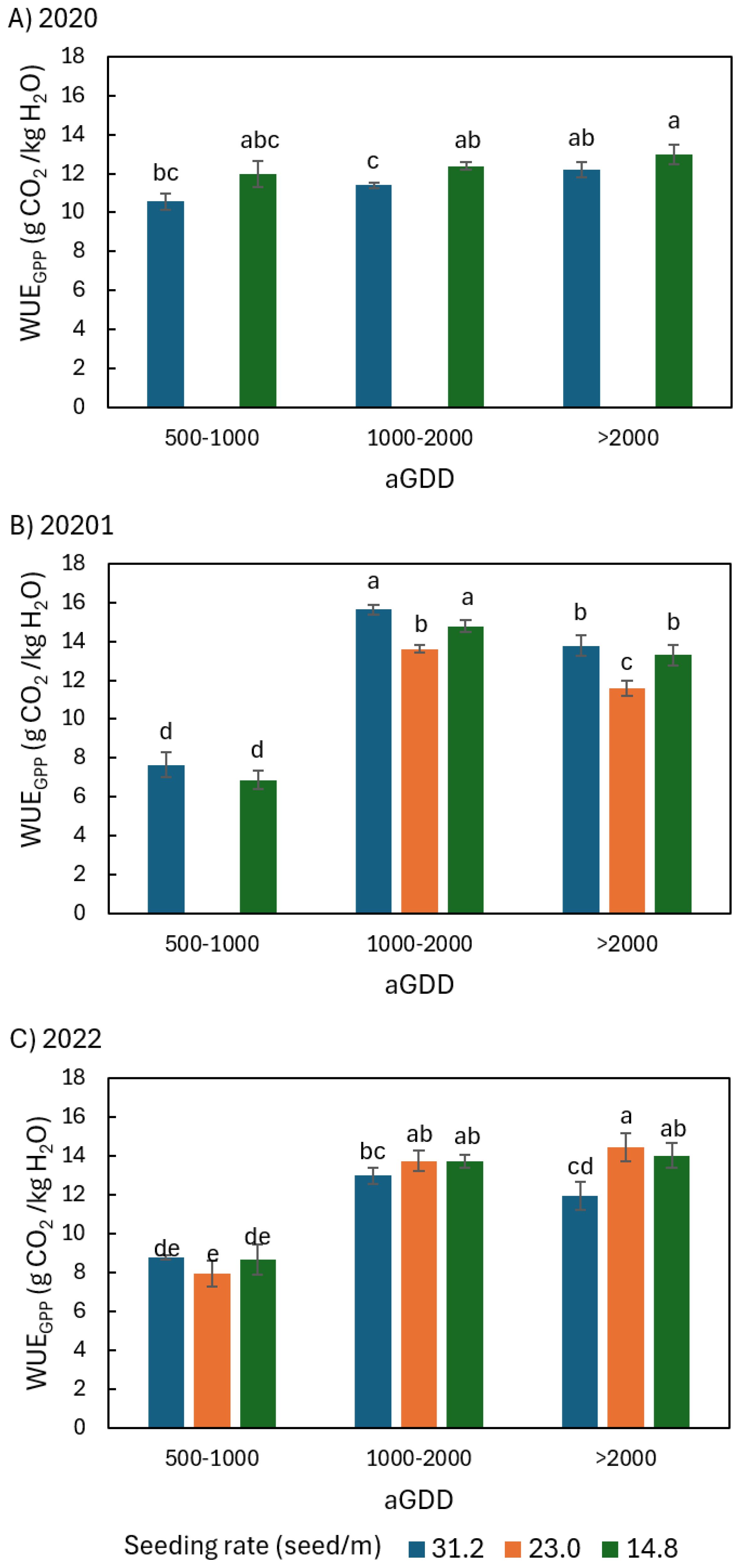
Figure 10. Comparison of the average daily peanut water-use efficiency (WUE) defined as the ratio of daily gross primary productivity (GPP) to evapotranspiration (ET), noted as WUE_GPP, among different seeding rates of 31.2, 23.0, and 14.8 seed/m during various ranges of accumulated growing degree day (aGDD) along the growing season in (A) 2020, (B) 2021, and (C) 2022, with error bars indicating the standard error of the mean and letters representing significant test results at the p = 0.1.

In 2020, both WUE_NEE,14.8 and WUE_GPP,14.8 tended to be larger than WUE_NEE,31.2 and WUE_GPP,31.2 by 6-17% and 6-13% in all aGDD ranges, respectively (Figures 9A, 10A). None of the differences were significant except for WUE_GPP during the aGDD 1000–2000 period.

In 2021, however, both WUE_NEE,31.2 and WUE_GPP,31.2 were larger than WUE_NEE,14.8 and WUE_GPP,14.8 by 4-27% and 4-11% throughout all aGDD ranges (Figures 9B, 10B), although only the differences in WUE_NEE during the periods of aGDD 500–1000 and 1000–2000 were significant. Moreover, both WUE_NEE,23.0 and WUE_GPP,23.0 were significantly the lowest among all seeding rates during aGDD 1000–2000 and aGDD > 2000.

Different from 2020 and 2021, WUE_NEE,14.8 in 2022 tended to be the lowest among all seeding rates during each aGDD range (Figure 9C). It is noted that WUE_NEE,14.8 during 500–1000 was extremely low, 65% and 70% lower than WUE_NEE,23.0 and WUE_NEE,31.2, respectively. Moreover, WUE_NEE,23.0 tended to be the highest among all seeding rates during aGDD 1000–2000 and aGDD > 2000. All the differences were basically non-significant except for WUE_NEE,23.0 being significantly higher than WUE_NEE,14.8 during aGDD 1000-2000.

WUE_GPP was different from WUE_NEE in 2022. During aGDD 500-1000, WUE_GPP,14.8 was equivalent to WUE_GPP,31.2 and 10% higher than the middle seeding rate 23.0 seed/m (Figure 10C). During both aGDD 1000–2000 and aGDD > 2000, however, WUE_GPP,31.2 tended to be the lowest in all three seeding rates, respectively. Moreover, while WUE_GPP,23.0 was equivalent to WUE_GPP,14.8 during aGDD 1000-2000, it tended to be the highest in all three seeding rates during aGDD > 2000.

3.6 Yield

Peanut yields with different seeding rates are compared in Figure 11. Peanut had the highest yield in 2021 and the lowest yield in 2022. The 23.0 seed/m seeding rate exhibited the largest yield of 8296 kg ha^-1 in 2021, but there were no significant yield differences among seeding rates in 2020 or 2022, although the seeding rate of 14.8 seed/m gave the non-significantly lowest yield in both 2020 and 2022, and 31.2 seed/m gave the non-significantly lowest yield in 2021.

Figure 11

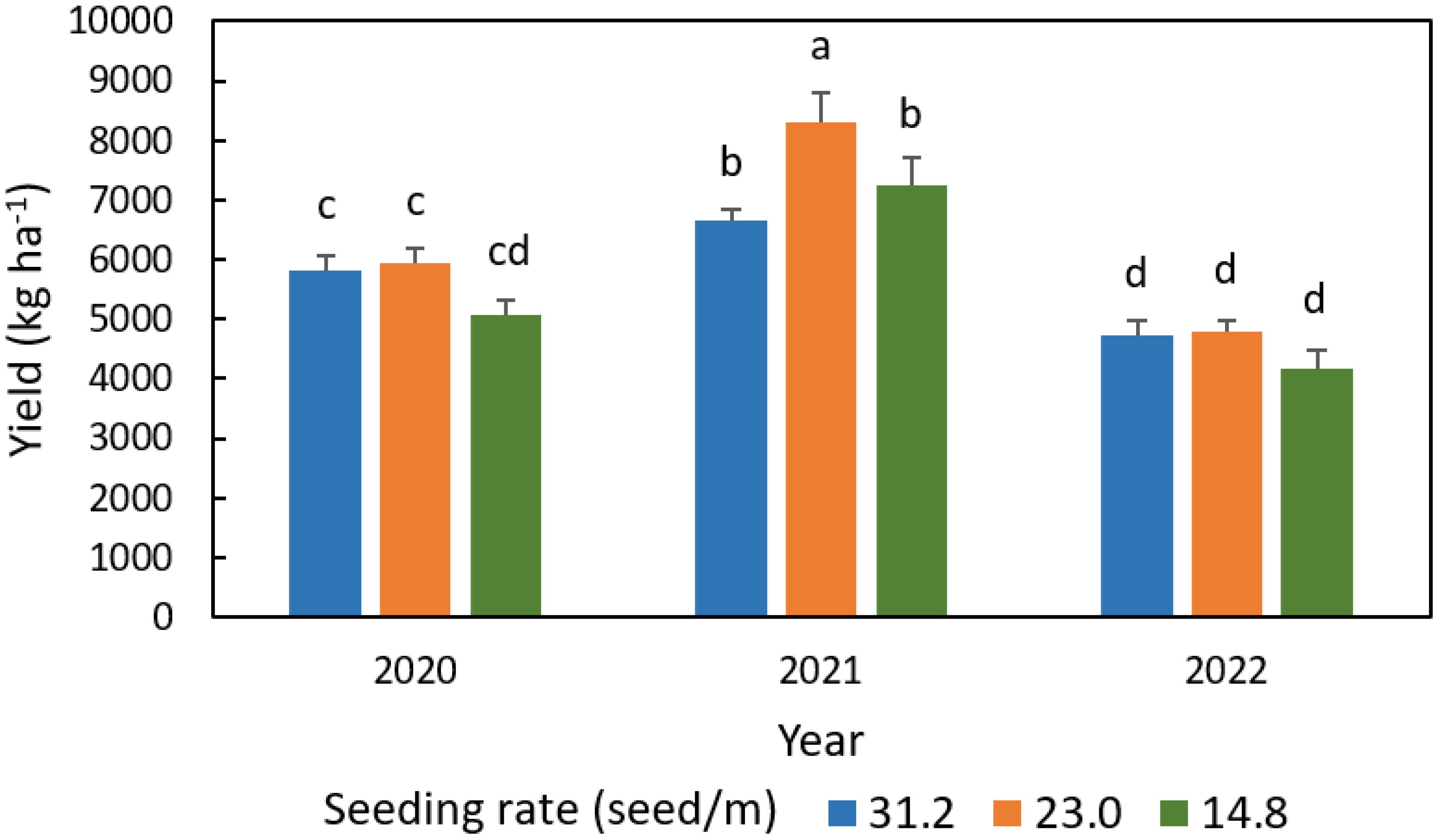
Figure 11. Comparison of peanut yield with different seeding rates in 2020, 2021, and 2022, with error bars indicating the standard error of the mean and letters representing significant test results at the p = 0.1.

4 Discussion

4.1 Ecosystem WUE, carbon budget and ET

The present study demonstrates how peanut properties NEE, GPP, R_e, ET, and WUE evolve throughout the different growth stages. Throughout the study, the lower values of these properties during the period of aGDD 500-1000 (corresponding to the period of beginning bloom – full pod, see Table 1) are mainly due to a lower LAI (Figure 4). As the LAI increases, the values of these properties increase and reach a maximum during aGDD 1000-2000 (beginning seed – beginning maturity). As for solar radiation, temperature, and LAI decrease during aGDD > 2000 (beginning maturity – harvest maturity), these properties values decrease, too. This is consistent with the behavior of daytime CO₂ fluxes, ET and WUE with growth stages reported by Zhang et al. (2022, 2023) and Bogati et al. (2023).

The impact of seeding rate on these attributes varies with weather conditions. In 2020 a typical year with average weather conditions, both WUE_NEE and WUE_GPP of 31.2 seed/m were lower than those of 14.8 seed/m, although the difference in WUE_NEE was not significant. This is because, although all the NEE, GPP, and ET of the higher seeding rate tended to be larger than those of the lower seeding rate, which was consistent with the difference in LAI between different seeding rates, the increment in ET of the high seeding rate compared to the ET of the lower seeding rates (Figure 8A) tended to be larger than the increments in NEE and GPP (Figures 5A, 6A) in the ‘normal’ weather conditions.

2021 was a wet year with more rainfall when aGDD > 500. Both WUE_NEE and WUE_GPP with the high seeding rate of 31.2 seed/m tended to be the largest in all three seeding rates in different growth stages, either significantly or not. This is because, in such a wet year, ET with the high seeding rate was the smallest in all seeding rates especially during both aGDD 1000–2000 and aGDD > 2000, more affected by the wet conditions than both GPP and NEE that were not significantly different among different seeding rates. However, both WUE_NEE and WUE_GPP of 23.0 seed/m were the lowest due to the highest ET among different seeding rates, possibly indicating peanut with the mid seeding rate is less affected by the wet conditions due to its moderate LAI. This variation may be related to the humidity and vapor pressure deficit in the canopy, both variables sensitive to the seeding rate and by extension the canopy density. Previous studies, such as Baldocchi (1994) in a wheat field; Law et al. (2002) at different flux sites in deciduous and evergreen forests, grasslands, crops, and tundra vegetation; Ponton et al. (2006) in a Douglas-fir forest, aspen (broad leaf deciduous) forest and wheatgrass (C₃) grassland; and Guo et al. (2022) in maize fields, all indicated that the ecosystem WUE decreased with vapor pressure deficit.

In 2022, WUE_NEE of 14.8 seed/m during aGDD 500–1000 was extremely low (-0.9 g CO₂/kg H₂O), the lowest among all seeding rates. This period experienced unusually high temperatures, vapor pressure deficit, and solar radiation, averaged at 27.3°C, 1.3 kPa, and 21.6 MJ m^-2 day^-1, respectively (Figure 3). The NEE of 14.8 seed/m was also extremely low, only -3.8 g CO₂ m^-2 day^-1 during this period (Figure 5C). This is due to its large R_e values (Figure 7C) resulting from high temperature and elevated vapor pressure deficit (Figures 3B, C), and moderate GPP (Figure 6C). Peanut leaves with low seeding rate intercept a higher solar radiation level per unit leaf area and thus higher local temperature and vapor pressure deficit than those with the higher seeding rates in early growing stages. This could be harmful to peanut growth in the abnormal higher air temperature and vapor pressure deficit conditions and thus increase its respiration and reduce NEE and WUE_NEE. The impact even influenced the next growth stage, leading to higher R_e and lower NEE and WUE_NEE. High temperature and vapor pressure deficit reducing WUE_NEE observed in 2022 in the current study is consistent to previous research. Craufurd et al. (1999) reported that high temperature decreases peanut WUE defined as the ratio of total dry matter accumulated between first flowering and harvest to total water use over the same period. Baldocchi (1994) indicated that the ecosystem WUE defined as the ratio of CO₂ flux to LE decreased with vapor pressure deficit in wheat field but not is a sparse corn field.

However, WUE_GPP of 14.8 seed/m in 2022 in the current study was like other seeding rates during aGDD 500-1000, and equivalent to that of 23.0 seed/m and higher than 31.2 seed/m during both aGDD 1000–2000 and aGDD > 2000. This is different from previous studies, which show that the ecosystem WUE defined as the ratio of GPP to ET is negatively related to vapor pressure deficit (Law et al., 2002; Ponton et al., 2006; Guo et al., 2022).

4.2 Yield

In contrast with the influence of seeding rate on WUE which varies with weather conditions and growth stages, the seeding rate of 23.0 seed/m exhibited the largest yield of all three treatments in 2021 and had equivalent yield to other seeding rates in 2020 and 2022 for different weather conditions. Of all three years, this makes it the overall best seeding rate for high yield. This is possibly because the mid seeding rate has a canopy with an optimum plant density with a lower competition for light, soil moisture and nutrient which would be present at higher density levels.

Such results for the seeding rate of 23.0 seed/m to tend to be the largest yield agree with those of Tubbs et al. (2011) who reported that the seeding rate of 17 seed/m exhibited lower yields than those higher seeding rates of 20 and 23 seed/m. Hagan et al. (2015) tested lower seeding rates from 6.6, 9.8, 13.1, and 19.7 seed/m. The Hagan et al. study also reported that higher seeding rates lead to higher yield. That may be because the range of seeding rates in the experiment were noticeably on the low side of the plant density scale. The 23.0 seed/m seeding rate is similar to the UGA Extension recommended seeding rate (UGA Extension, 2022). The present findings support the UGA Extension recommendation and demonstrate that there is an optimum seeding rate potentially avoiding lower yield for seeding rates that are either higher or lower than the recommended rate.

The yield results combined with the WUE results in the current study indicate that the high WUE with high yield can be achieved with mid seeding rate in a hot dry year, while the high WUE and high yield may not be simultaneously obtained by the seeding rate in a wet year.

5 Conclusions

This paper has examined the influence of three seeding rates of 14.8, 23.0, and 31.2 seed/m on peanut ecosystem water-use efficiency (WUE). The latter was determined by the ratio of the net CO₂ exchange to the evapotranspiration (ET) measured. Both are obtained using the eddy-covariance method, a technique capturing fluxes at the field scale and continuously round the clock throughout all growth stages over a three-year study period. This approach constitutes a considerable improvement over traditional methods that use discrete measurements and typical small agronomic-size plots.

Results suggest that the influence of seeding rate on WUE is closely coupled to weather conditions. In 2020, a season with ‘normal’ weather conditions, both the WUE as the ratio of net ecosystem exchange of CO₂ (NEE) to ET (WUE_NEE) and the WUE as the ratio of gross primary productivity (GPP) to ET (WUE_GPP) for the low seeding rate of 14.8 seed/m tended to be larger than those for high seeding rate of 31.2 seed/m by 6-17% and 6-13% throughout all accumulated Growing Degree Day (aGDD) ranges, respectively. This is because the increment in ET of the high seeding rate compared to that of the low seeding rates tended to be larger than the increments in NEE and GPP.

In 2021, a particularly wet season with more rainfall, both WUE_NEE and WUE_GPP in the high seeding rate were larger than those with lower seeding rates. This is attributed to the fact that ET in the high seeding rate was hindered more than those in lower seeding rates in such wet conditions as the dense canopy prevented the lower canopy layers from drying quickly the way a canopy with a lower seeding rate would.

2022 was a year characterized by abnormally hot and dry year specially throughout the early growing season (aGDD 500-1000, the period of beginning bloom – full pod). These conditions resulted in high respiratory losses and considerably low NEE in the low seeding rate field compared to both higher seeding rate fields. This leads to the WUE_NEE with the low seeding rate being 65% and 70% lower than the higher seeding rates during aGDD 500–1000 respectively, while WUE_GPP with the low seeding rate was equivalent to that with the higher seeding rates.

Of all three experimental years, peanut had the highest yield in the wet year of 2021 and the lowest yield in 2022 with abnormally hot and dry conditions. Peanut with the mid seeding rate had the greatest yield amongst the three seeding rate treatments in 2021 of wet season and had yield equivalent to other seeding rates in the other two years. The mid seeding rate is thus considered to be the best option to get the overall highest yield. This result further corroborates the University of Georgia Extension recommendation.

In the current study, combining both the yield and WUE results, the highest WUE with high yield is achieved using the mid seeding rate in a hot dry year. However, high WUE with high yield might not be obtained by selecting the seeding rate in a wet year. Thus, the results reported in this paper concur with the Peanut Rx, i.e., the mid seeding rate is recommended to obtain high yield with high WUE. Our data further support the assertion that regardless of whether the growing season is predicted to be dry or wet, the mid seeding rate is the indicated choice: In a forecast of a rainy year, the mid seeding rate is expected to still produce high yield, though its WUE would not be as high as the other seeding rates, but WUE is not that important in a rainy year.

Data availability statement

The raw data supporting the conclusions of this article will be made available by the authors, without undue reservation.

Author contributions

GZ: Data curation, Formal analysis, Methodology, Writing – original draft, Writing – review & editing. ML: Conceptualization, Funding acquisition, Methodology, Writing – original draft, Writing – review & editing. KP: Data curation, Formal analysis, Writing – original draft. RT: Data curation, Funding acquisition, Writing – review & editing. WM: Funding acquisition, Writing – review & editing.

Funding

The author(s) declare that financial support was received for the research and/or publication of this article. Georgia Peanut Commission supported the research funding for this project.

Acknowledgments

The authors would like to thank the farm crew at the Southwest Georgia Research and Education Center, the University of Georgia, Plains, GA USA.

Conflict of interest

The authors declare that the research was conducted in the absence of any commercial or financial relationships that could be construed as a potential conflict of interest.

Generative AI statement

The author(s) declare that no Generative AI was used in the creation of this manuscript.

Publisher’s note

All claims expressed in this article are solely those of the authors and do not necessarily represent those of their affiliated organizations, or those of the publisher, the editors and the reviewers. Any product that may be evaluated in this article, or claim that may be made by its manufacturer, is not guaranteed or endorsed by the publisher.

References

Anderson R., Wang D., Skaggs T., Alfieri J., Scanlon T. M., and Kustas W. (2017). Impact of water use efficiency parameterization on partitioning evapotranspiration (ET) with the eddy covariance flux variance method. ASA CSSA SSSA Int. Annu.

Google Scholar

Angevine W. M., Edwards J. M., Lothon M., LeMone M. A., and Osborne S. R. (2020). Transition periods in the diurnally-varying atmospheric boundary layer over land. Boundary-Layer. Meteorology 177, 205–223. doi: 10.1007/s10546-020-00515-y

Crossref Full Text | Google Scholar

Bakal H., Kenetli A., and Arioglu H. (2020). The effect of plant density on pod yield and some agronomic characteristics of different growthtype peanut varieties (Arachis hypogaea L.) grown as a main crop. Turk J. Field Crops 25, 92–99. doi: 10.17557/tjfc.748671

Crossref Full Text | Google Scholar

Baldocchi D. (1994). A comparative study of mass and energy exchange rates over a closed C3 (wheat) and an open C4 (corn) crop: II. CO2 exchange and water use efficiency. Agric. For. Meteorol. 67, 291–321. doi: 10.1016/0168-1923(94)90008-6

Crossref Full Text | Google Scholar

Baldocchi D., Ma S., and Verfaillie J. (2021). On the inter- and intra-annual variability of ecosystem evapotranspiration and water use efficiency of an oak savanna and annual grassland subjected to booms and busts in rainfall. Glob Change Biol. 27, 359–375. doi: 10.1111/gcb.15414

PubMed Abstract | Crossref Full Text | Google Scholar

Beasley J. P. (2013). “Cultivar options in 2013,” in 2013 Peanut Production Update. Ed. Beasley J. P. (Athens, GA, USA: Univ. of Georgia Coop. Ext. Serv.), 55–56. Available at: http://flacrops.com/wp-content/uploads/2013/04/2013UGAPeanutProductionGuide.pdf (Accessed March 18, 2025).

Google Scholar

Black M. C., Tewolde H., Fernandez C. J., and Schubert A. M. (2001). Seeding rate, irrigation, and cultivar effects on tomato spotted wilt, rust, and southern blight diseases of peanut. Peanut Sci. 28, 1–4. doi: 10.3146/i0095-3679-28-1-1

Crossref Full Text | Google Scholar

Bogati S., Leclerc M. Y., Zhang G., Kaur Brar S., Tubbs R. S., Monfort W. S., et al. (2023). The impact of tillage practices on daytime CO₂ fluxes, evapotranspiration (ET), and water-use efficiency in peanut. Frontiers in Agronomy. Sec. Climate-Smart Agron. 5. doi: 10.3389/fagro.2023.1228407

Crossref Full Text | Google Scholar

Boote K., Stansell J. R., Schubert A. M., and Stone J. F. (1982). “Irrigation, water use, and water relations,” in Peanut science and technology. Eds. Patte H. E. and Young C. T. (Youkam, Texas: American Peanut Research and Education Association), 164–205.

Google Scholar

Branch W. D. (2007). Registration of 'Georgia-06G'peanut. J. Plant Registr. 1, 120–120. doi: 10.3198/jpr2006.12.0812crc

Crossref Full Text | Google Scholar

Branch W. D., Baldwin J. A., and Culbreath A. K. (2003). Genotype X seeding rate interaction among TSWV-resistant, runner-type peanut cultivars. Peanut Sci. 30, 108–111. doi: 10.3146/pnut.30.2.0009

Crossref Full Text | Google Scholar

Craufurd P. Q., Wheeler T. R., Ellis R. H., Summerfield R. J., and Williams J. H. (1999). Effect of temperature and water deficit on water-use efficiency, carbon isotope discrimination, and specific leaf area in peanut. Crop Sci. 39, 136–142. doi: 10.2135/cropsci1999.0011183X003900010022x

Crossref Full Text | Google Scholar

Dekker S. C., Groenendijk M., Booth B. B., Huntingford C., and Cox P. M. (2016). Spatial and temporal variations in plant water-use efficiency inferred from tree-ring, eddy covariance and atmospheric observations. Earth Sys. Dynam. 7, 525–533. doi: 10.5194/esd-7-525-2016

Crossref Full Text | Google Scholar

EddyPro (2019). EddyPro, version 7.0.3 (Lincoln, NE, USA: LI-COR biosciences).

Google Scholar

Ekram A. M., Mekdad A. A. A., and El Damy H. M. (2019). Response of ground nut (Arachis Hypogaea, L.) to different sowing dates and seeding rates in newly reclaimed land. Fayoum J. Agric. Res. Dev. 33, 61–71. doi: 10.21608/fjard.2019.190563

Crossref Full Text | Google Scholar

Engström J., Praskievicz S., Bearden B., and Moradkhani H. (2021). Decreasing water resources in Southeastern US as observed by the GRACE satellites. Water Policy 23, 1017–1029. doi: 10.2166/wp.2021.039

Crossref Full Text | Google Scholar

Falge E., Baldocchi D., Olson R., Anthoni P., Aubinet M., Bernhofer C., et al. (2001). Gap filling strategies for defensible annual sums of net ecosystem exchange. Agric. For. Meteorol. 107, 43–69. doi: 10.1016/S0168-1923(00)00225-2

Crossref Full Text | Google Scholar

Fill J. M., Davis C. N., and Crandall R. M. (2019). Climate change lengthens southeastern USA lightning-ignited fire seasons. Global Change Biol. 25, 3562–3569. doi: 10.1111/gcb.14727

PubMed Abstract | Crossref Full Text | Google Scholar

Golladay S. W., Gagnon P., Kearns M., Battle J. M., and Hicks D. W. (2004). Response of freshwater mussel assemblages (Bivalvia: Unionidae) to a record drought in the Gulf Coastal Plain of southwestern Georgia. J. North Am. Benthol. Soc. 23, 494–506. doi: 10.1899/0887-3593(2004)023<0494:ROFMAB>2.0.CO;2

Crossref Full Text | Google Scholar

Google Earth Pro (2019). Google Earth pro, version 7.3 (Mountain View, CA, USA: Google LLC).

Google Scholar

Guo H., Li S., Kang S., Du T., Liu W., Tong L., et al. (2022). The controlling factors of ecosystem water use efficiency in maize fields under drip and border irrigation systems in Northwest China. Agric. Water Manage. 272, 107839. doi: 10.1016/j.agwat.2022.107839

Crossref Full Text | Google Scholar

Hagan A. K., Campbell H. L., Bowen K. L., and Wells L. (2015). Seeding rate and planting date impacts stand density, diseases, and yield of irrigated peanuts. Plant Health Prog. 16, 64–70. doi: 10.1094/PHP-RS-14-0019

Crossref Full Text | Google Scholar

Helbig M., Gerken T., Beamesderfer E. R., Baldocchi D. D., Tirtha Banerjee T., Biraud S. C., et al. (2021). Integrating continuous atmospheric boundary layer and tower-based flux measurements to advance understanding of land-atmosphere interactions. Agric. For. Meteorol. 307, 108509. doi: 10.1016/j.agrformet.2021.108509

Crossref Full Text | Google Scholar

Hoover D. L., Abendroth L. J., Browning D. M., Saha A., Snyder K., and Wagle P. (2023). Indicators of water use efficiency across diverse agroecosystems and spatiotemporal scales. Sci. Total Environ. 864, 160992. doi: 10.1016/j.scitotenv.2022.160992

PubMed Abstract | Crossref Full Text | Google Scholar

IPCC and Core Writing Team (2023). Climate Change 2023: Synthesis Report. Contribution of Working Groups I, II and III to the Sixth Assessment Report of the Intergovernmental Panel on Climate Change. Eds. Lee H. and Romero J. (Geneva, Switzerland: IPCC), 184. doi: 10.59327/IPCC/AR6-9789291691647

Crossref Full Text | Google Scholar

Konlan S., Sarkodie-Addo J., Asare E., Kombiok M. J., and Adu-Dapaah H. (2014). Effect of seeding rate on productivity and profitability of groundnut (Arachis hypogaea L.). J. Exp. Biol. Agric. Sci. 2, 83–89.

Google Scholar

Kormann R. and Meixner F. X. (2001). An analytical footprint model for non-neutral stratification. Boundary-Layer Meteorol. 99, 207–224. doi: 10.1023/A:1018991015119

PubMed Abstract | Crossref Full Text | Google Scholar

Law B. E., Falge E., Gu L., Baldocchi D. D., Bakwin P., Berbigier P., et al. (2002). Environmental controls over carbon dioxide and water vapor exchange of terrestrial vegetation. Agric. For. Meteorol. 113, 97–120. doi: 10.1016/S0168-1923(02)00104-1

Crossref Full Text | Google Scholar

Leclerc M. Y. and Foken T. (2014). Footprints in micrometeorology and ecology (Berlin, Heidelberg, Germany: Springer), 1–239.

Google Scholar

Leclerc M. and Thurtell G. (1990). Footprint prediction of scalar fluxes using a Markovian analysis. Boundary-Layer Meteorol. 52, 247–258. doi: 10.1007/BF00122089

Crossref Full Text | Google Scholar

Lloyd J. and Taylor J. A. (1994). On the temperature dependence of soil respiration. Funct. Ecol. 8, 315–323. doi: 10.2307/2389824

Crossref Full Text | Google Scholar

Mauder M. and Foken T. (2006). Impact of post-field data processing on eddy covariance flux estimates and energy balance closure. Meteorol. Z. 15, 597–609. doi: 10.1127/0941-2948/2006/0167

Crossref Full Text | Google Scholar

McCombs A. G., Hiscox A. L., and Suyker A. E. (2019). Point-to-grid conversion in flux footprints: implications of method choice and spatial resolution for regional-scale studies. Boundary-Layer Meteorol. 172, 457–479. doi: 10.1007/s10546-019-00455-2

Crossref Full Text | Google Scholar

Mills W. T. (1964). Heat unit system for predicting optimum peanut harvesting time. Trans. ASAE 7, 307–309,312. doi: 10.5555/19651701356

Crossref Full Text | Google Scholar

Minton N. A. and Csinos A. S. (1986). Effects of row spacings and seeding rates of peanut on nematodes and incidence of southern stem rot. Nematropica 16, 167–176. doi: 10.5555/19870839429

Crossref Full Text | Google Scholar

Moffat A. M., Papale D., Reichstein M., Hollinger D. Y., Richardson A. D., Barr A. G., et al. (2007). Comprehensive comparison of gap-filling techniques for eddy covariance net carbon fluxes. Agric. For. Meteorol. 147, 209–232. doi: 10.1016/j.agrformet.2007.08.011

Crossref Full Text | Google Scholar

Monfort W. S. (2017). “Peanut cultivar options,” in 2017 Peanut Update. Ed. Monfort W. S. (Athens, GA, USA: Univ. of Georgia Coop. Ext. Serv.), 4–11.

Google Scholar

Morla F. D., Giayetto O., Fernandez E. M., Cerioni G. A., and Cerliani C. (2018). Plant density and peanut crop yield (Arachis hypogaea) in the peanut growing region of Córdoba (Argentina). Peanut Sci. 45, 82–86. doi: 10.3146/0095-3679-45.2.82

Crossref Full Text | Google Scholar

Nahrawi H., Leclerc M. Y., Pennings S., Zhang G., Singh N., and Pahari R. (2020). Impact of tidal inundation on the net ecosystem exchange in daytime conditions in a salt marsh. Agric. For. Meteorol. 294, 108133. doi: 10.1016/j.agrformet.2020.108133

Crossref Full Text | Google Scholar

Niu S., Xing X., Zhang Z., Xia J., Zhou X., Song B., et al. (2011). Water-use efficiency in response to climate change: from leaf to ecosystem in a temperate steppe. Global Change Biol. 17, 1073–1082. doi: 10.1111/j.1365-2486.2010.02280.x

Crossref Full Text | Google Scholar

NOAA (National Oceanic and Atmospheric Administration) (2021). Fourth national climate assessment. Our changing Climate 2, 74–76. Available online at: https://nca2018.globalchange.gov/downloads/NCA4_Ch00_Front-Matter.pdf.

Google Scholar

Oakes J. C., Balota M., Jordan D. L., Hare A. T., and Sadeghpour A. (2020). Peanut response to seeding density and digging date in the Virginia-Carolina region. Peanut Sci. 47, 180–188. doi: 10.3146/PS20-16.1

Crossref Full Text | Google Scholar

Paharia R., Leclerca M. Y., Zhang G., Nahrawi H., and Raymerc P. (2018). Carbon dynamics of a warm season turfgrass using the eddy-covariance technique. Agricult. Ecosys. Environ. 251, 11–25. doi: 10.1016/j.agee.2017.09.015

Crossref Full Text | Google Scholar

Ponton S., Flanagan L. B., Alstad K. P., Johnson B. G., Morgenstern K., Kljun N., et al. (2006). Comparison of ecosystem water-use efficiency among douglas-fir forest, aspen forest and grassland using eddy covariance and carbon isotope techniques. Global Change Biol. 12, 294–310. doi: 10.1111/j.1365-2486.2005.01103.x

Crossref Full Text | Google Scholar

RStudio (2024). RStudio: Integrated Development Environment for R (Boston, MA: RStudio, PBC). Available online at: https://posit.co.

Google Scholar

Reichstein M., Falge E., Baldocchi D., Papale D., Aubinet M., Berbigier P., et al. (2005). On the separation of net ecosystem exchange into assimilation and ecosystem respiration: review and improved algorithm. Global Change Biol. 11, 1424–1439. doi: 10.1111/j.1365-2486.2005.001002.x

Crossref Full Text | Google Scholar

Reichstein M. and Moffet A. M. (2015). REddyProc: Data Processing and Plotting Utilities of (half-)hourly Eddy-covariance Measurements, R Package Version 0.7-1/r13 (Jena, Germany: Max Plant Institute for Biogeochemistry).

Google Scholar

Rowland D., Sorensen R., Butts C., and Faircloth W. (2006). Determination of maturity and degree day indices and their success in predicting peanut maturity. Peanut Sci. 33, 125–136. doi: 10.3146/0095-3679(2006)33[125:DOMADD]2.0.CO;2

Crossref Full Text | Google Scholar

Scanlon T. M. and Albertson J. D. (2004). Canopy scale measurements of CO2 and water vapor exchange along a precipitation gradient in southern Africa. Global Change Biol. 10, 329–341. doi: 10.1046/j.1365-2486.2003.00700.x

Crossref Full Text | Google Scholar

Smith N. B. and Smith A. R. (2010). “Peanut outlook and cost analysis for 2010,” in J 2010 Peanut Update. Ed. Beasley P. Jr. (Univ. of Georgia Coop. Ext. Serv., Athens, GA), 3–14 (Accessed June 20, 2024).

Google Scholar

Smith N. B. and Smith A. (2012). “Peanut Production Budgets,” in 2012 Peanut Production Update. Ed. Beasley J. P. (Univ. of Georgia Coop. Ext. Serv., Athens, GA). Available at: http://www.caes.uga.edu/commodities/fieldcrops/peanuts/documents/2012PeanutProductionUpdateGuide.pdf.

Google Scholar

Sorensen R. B., Lamb M. C., and Butts C. L. (2007). Peanut response to row pattern and seed density when irrigated with subsurface drip irrigation. Peanut Sci. 34, 27–31. doi: 10.3146/0095-3679(2007)34[27:PRTRPA]2.0.CO;2

Crossref Full Text | Google Scholar

Sorensen R. B., Sconyers L. E., Lamb M. C., and Stemitzke D. A. (2004). Row orientation and seeding rate on yield, grade, and stem rot incidence of peanut with subsurface drip irrigation. Peanut Sci. 31, 54–58. doi: 10.3146/pnut.31.1.0012

Crossref Full Text | Google Scholar

Sujathamma P. and Santhosh Kumar Naik B. (2022). Response of groundnut varieties to different seed rates. Pharma Innovation J. 11, 956–959.

Google Scholar

Sun G. (2013). Impacts of Climate Change and Variability on Water Resources in the Southeast USA. In: Ingram K. T., Dow K., Carter L., and Anderson J. (eds) Climate of the Southeast United States. NCA Regional Input Reports. Washington, DC: Island Press. doi: 10.5822/978-1-61091-509-0_10

Crossref Full Text | Google Scholar

Tallarita A., Sannino M., Cozzolino E., Albanese D., Fratianni F., Faugno S., et al. (2021). Yield, quality, antioxidants and elemental composition of peanut as affected by plant density and harvest time. Italus Hortus 28, 25–35. doi: 10.26353/j.itahort/2021.3.2535

Crossref Full Text | Google Scholar

Tallec T., Béziat P., Jarosz N., Rivalland V., and Ceschia E. (2013). Crops’ water use efficiencies in temperate climate: Comparison of stand, ecosystem and agronomical approaches. Agric. For. Meteorol. 168, 69–81. doi: 10.1016/j.agrformet.2012.07.008

Crossref Full Text | Google Scholar

Tewolde H., Black M. C., Fernandez C. J., and Schubert A. M. (2002). Plant growth response of two runner peanut cultivars to reduced seeding rate. Peanut Sci. 29, 8–12. doi: 10.3146/pnut.29.1.0002

Crossref Full Text | Google Scholar

Tubbs R. S., Beasley J. P. Jr., Culbreath A. K., Kemerait R. C., Smith N. B., and Smith A. R. (2011). Row pattern and seeding rate effects on agronomic, disease, and economic factors in large-seeded runner peanut. Peanut Sci. 38, 93–100. doi: 10.3146/PS10-19.1

Crossref Full Text | Google Scholar

UGA Extension (2022). Peanut Production Guide (Athens, GA: University of Georgia Extension Bulletin 1146), 178. Available at: https://secure.caes.uga.edu/extension/publications/files/pdf/B%201146_2.PDF (Accessed December 18, 2024).

Google Scholar

USDA/NASS (2024). USDA/NASS Crop Production 2023 Summary (Washington, DC: National Agricultural Statistics Service, United States Department of Agriculture (USDA)).

Google Scholar

Vickers D. and Mahrt L. (1997). Quality control and flux sampling problems for tower and aircraft data. J. Atmos. Ocean. Technol. 14, 512–526. doi: 10.1175/1520-0426(1997)014<0512:QCAFSP>2.0.CO;2

Crossref Full Text | Google Scholar

Vörösmarty C. J., Green P., Salisbury J., and Lammers R. B. (2000). Global water resources: vulnerability from climate change and population growth. Science 289, 284–288. doi: 10.1126/science.289.5477.284

PubMed Abstract | Crossref Full Text | Google Scholar

Wagle P., Skaggs T. H., Gowda P. H., Northup B. K., and Neel J. P. (2020). Flux variance similarity-based partitioning of evapotranspiration (ET) over a rainfed alfalfa field using high frequency eddy covariance data. Agric. For. Meteorol. 285, 107907. doi: 10.1016/j.agrformet.2020.107907

Crossref Full Text | Google Scholar

Wang T., Tang X., Zheng C., Gu Q., Wei J., and Ma M. (2018). Differences in ecosystem water-use efficiency among the typical croplands. Agric. Water Manage. 209, 142–150. doi: 10.1016/j.agwat.2018.07.030

Crossref Full Text | Google Scholar

Webb E. K., Pearman G. I., and Leuning R. (1980). Correction of flux measurements for density effects due to heat and water vapour transfer. Q. J. R. Meteorol. Soc. 106, 85–100. doi: 10.1002/qj.49710644707

Crossref Full Text | Google Scholar

Wehtje G., Weeks R., West M., Wells L., and Pace P. (1994). Influence of planter type and seeding rate on yield and disease incidence in peanut. Peanut Sci. 21, 16–19. doi: 10.3146/i0095-3679-21-1-5

Crossref Full Text | Google Scholar

Wilczak J. M., Oncley S. P., and Stage S. A. (2001). Sonic anemometer tilt correction algorithms. Boundary-Layer Meteorol. 99, 127–150. doi: 10.1023/A:1018966204465

Crossref Full Text | Google Scholar

Williams R. B., Al-Hmoud R., Segarra E., and Mitchell D. (2017). An estimate of the shadow price of water in the southern Ogallala Aquifer. J. Water Res. Prot. 9, 289–304. doi: 10.4236/jwarp.2017.93019

Crossref Full Text | Google Scholar

Williams E. J. and Drexler J. S. (1981). A non-destructive method for determining peanut pod maturity. Peanut Sci. 8, 134–141. doi: 10.3146/i0095-3679-8-2-15

Crossref Full Text | Google Scholar

Zhang G., Leclerc M. Y., Singh N., Tubbs R. S., and Monfort W. S. (2022). Impact of planting date on CO₂ fluxes, evapotranspiration and water-use efficiency in peanut using the eddy-covariance technique. Agric. For. Meteorol. 326, 109163. doi: 10.1016/j.agrformet.2022.109163

Crossref Full Text | Google Scholar

Zhang G., Leclerc M. Y., Singh N., Tubbs R. S., and Montfort W. S. (2023). Influence of planting pattern on peanut daytime net carbon uptake, evapotranspiration, and water-use efficiency using the eddy-covariance method. Frontiers in agronomy. Sec. Climate-Smart Agron. 5, 1–12. doi: 10.3389/fagro.2023.1204887

Crossref Full Text | Google Scholar

Zhao F.-H., Yu G.-R., Li S.-G., Ren C.-Y., Sun X.-M., Mi N., et al. (2007). Canopy water use efficiency of winter wheat in the North China Plain. Agric. Water Manage. 93, 99–108. doi: 10.1016/j.agwat.2007.06.012

Crossref Full Text | Google Scholar