Modeling soil water dynamics to optimize blueberry irrigation in sandy soils

Introduction: Drip irrigation is widely used by growers to improve application efficiency in high-value crops such as blueberry, where efficient water management is critical. Optimizing soil moisture conditions in blueberry production systems through irrigation system design is of particular importance, as blueberries are typically grown in sandy soils and have a shallow root system. In addition, climate variability in blueberry production regions has complicated irrigation management. The objective of this work was to optimize drip irrigation system design and management practice using the HYDRUS 2D model.

Methods: Field soil moisture and environmental conditions were monitored using a Sentek Drill & Drop soil moisture sensor system installed at nine depths within the root zone during 2024 growing season in Michigan. The collected field data were used to calibrate The HYDRUS 2D model to simulate soil water distribution under drip irrigation. During calibration, the standard statistical indicators used were Nash–Sutcliffe efficiency (NSE), index of agreement (IA), and root mean square error (RMSE), with values of >0.93, >0.98, and <0.03 cm³/cm³, respectively. Four numerical experiments were conducted in HYDRUS 2D to optimize drip irrigation system management. These experiments included evaluating the impact of 1) irrigation application system (single vs. double drip lines), 2) emitter spacing (15-, 30-, 45-, 60-cm), 3) irrigation duration (1-, 0.5-, 0.25- hour), and 4) emitter flow rate (0.98 L/h, 1.89 L/h).

Results: A single drip line, emitter spacing of 45 or 60 cm, a 0.5-hour irrigation duration, and a flow rate of 1.89 L/h optimized irrigation application efficiency and minimized the risk of leaching water below the root zone. In addition, result indicated that in both single and double drip line systems, higher emitter flow rates enhanced soil moisture availability within the root zone. However, longer irrigation durations, such as 1 hour significantly increased the risk of water percolating beyond the effective root depth, particularly in sandy soils. Future research will evaluate alternative modeling approaches and validate the methodology across diverse soil and climate conditions to enhance robustness.

Discussion: Overall, the results indicate that the HYDRUS-2D model is a reliable and effective tool for optimizing the design and management of drip irrigation systems in blueberry production. By simulating the dynamic movement of water within the root zone, the model helps identify irrigation conditions that optimize water use efficiency while reducing the risk of water leaching beyond the effective root depth.

1 Introduction

Drip irrigation is commonly used in vegetable and fruit production systems to increase application efficiency while minimizing the loss of irrigation water through evaporation (Bravdo and Proebsting, 2018). Drip irrigation systems typically improve irrigation application efficiency when compared to sprinkler irrigation systems. Under drip irrigation, water flows slowly to plant roots from above the soil surface, potentially conserving water and nutrients. As it does not have any contact with plant leaves, the spread of diseases could be prevented. This method is effective as it can save water (Bhavsar et al., 2023). Multiple studies have shown that drip irrigation reduces water use by an average of 28%–55% compared to other forms of irrigation (Lamm and Trooien, 2003). However, this range may vary based on factors such as crop type, soil properties, and environmental conditions, and more precise estimates can be achieved through site-specific studies. Blueberry plants have shallow root systems and prefer to grow in well-drained, sandy soils (Egea et al., 2017). Michigan is a major blueberry-producing state, with nearly 6,900 ha producing over 39,000 metric tons of blueberries in 2023 (USDA-NASS, 2023). Most blueberry fields in Michigan are located on the west side of the State due to the moderating effect of Lake Michigan on winter temperatures (Kovach, 2006). The majority of irrigated fields in Michigan are mainly comprised of coarse-textured soils such as sand, loamy sand, and sandy loam (Dong et al., 2024). Maintaining optimal moisture levels within the shallow root zone of blueberry plants grown in sandy soils presents a major challenge for blueberry growers to properly and efficiently optimize irrigation water (Goldy, 2012). Over-irrigation is a common issue, and this wastes water resources and increases the risk of nutrient leaching, which could flow into groundwater (Dong, 2022). Drip irrigation systems are becoming increasingly adopted by Michigan blueberry growers to increase irrigation application efficiency and mitigate the effects of erratic precipitation.

Computational modeling is a tool that can assist with understanding water flow in soil through simulation. Many computational models are available to simulate water flow in soils, such as HYDRUS (Dong et al., 2019a), Leaching Estimation and Chemistry Model (LEACHM) (Puertes et al., 2019), DRAINMOD (Moursi et al., 2022), WASH_2D (Liang et al., 2022), SALTMED (Feng et al., 2024), and Soil-Water-Atmosphere-Plant (SWAP) (van Dam et al., 2008). Of these models, HYDRUS has been used extensively to simulate water flow in drip irrigation systems (Elnesr and Alazba, 2019). In addition to water flow, HYDRUS-2D was also utilized to observe carbon degradation and nitrogen transformation in soils (Dong et al., 2019b). HYDRUS-2D is a two-dimensional finite element model. It has been utilized to simulate both lateral and vertical water flow from a drip emitter and the subsequent changes in soil moisture content (Surendran and Madhava Chandran, 2022). A comparison of a HYDRUS-2D simulation with observations from a field experiment under a drip irrigation system was conducted and showed a strong relationship between simulated and field-measured values (Skaggs et al., 2004). HYDRUS-2D also successfully simulated the range and pattern of soil water content fluctuation in a drip-irrigated cotton field (Bufon et al., 2012). Moreover, Honari et al. (2017) agreed that HYDRUS-3D successfully simulated soil moisture level changes in drip-irrigated corn and wheat fields (Honari et al., 2017). Because of its accurate reflection of soil water flow, HYDRUS-2D has been proposed as a useful model in designing and developing drip irrigation systems (Kandelous and Šimůnek, 2010). While previous studies have primarily focused on HYDRUS-2D simulations under controlled environments or limited weather scenarios (Li et al., 2023; Cordel et al., 2025), there is little knowledge on applying the HYDRUS model for site-specific irrigation management of blueberry, a crop with sensitive water requirements and significant economic value. This study takes a unique approach by also modeling the effect of varying climate conditions experienced in a commercial blueberry field. Therefore, the objectives of this study were to 1) monitor soil water flow in a blueberry field, 2) calibrate the HYDRUS-2D model using field data, and 3) utilize the calibrated model to simulate different irrigation approaches and climate conditions to maintain the optimal moisture levels for blueberry plants grown in sandy soils.

2 Materials and methods

2.1 Field data collection

The field experiment data were collected in a ‘Duke’ blueberry field in West Olive, MI, USA (Figure 1A). This farm uses a single-line polyethylene drip irrigation system, which has pressure-compensated emitters spaced at 60 cm. Water flow rate was measured by placing a 10.16-cm PVC cap (catch can) under multiple emitters (Figure 1B). The flow was evaluated at 35 emitters, and the average flow rate was 1.89 L/h. Water pressure was measured at the end of the row using a pressure gauge to ensure the irrigation system maintains the correct pressure throughout the system. A blue dye test was conducted by injecting blue dye into a drip line to evaluate the area the water from a single emitter affects (Figure 1C) (Simonne et al., 2004). Weather data were collected using the Michigan State University Enviroweather station in Grand Junction, Michigan.

Figure 1

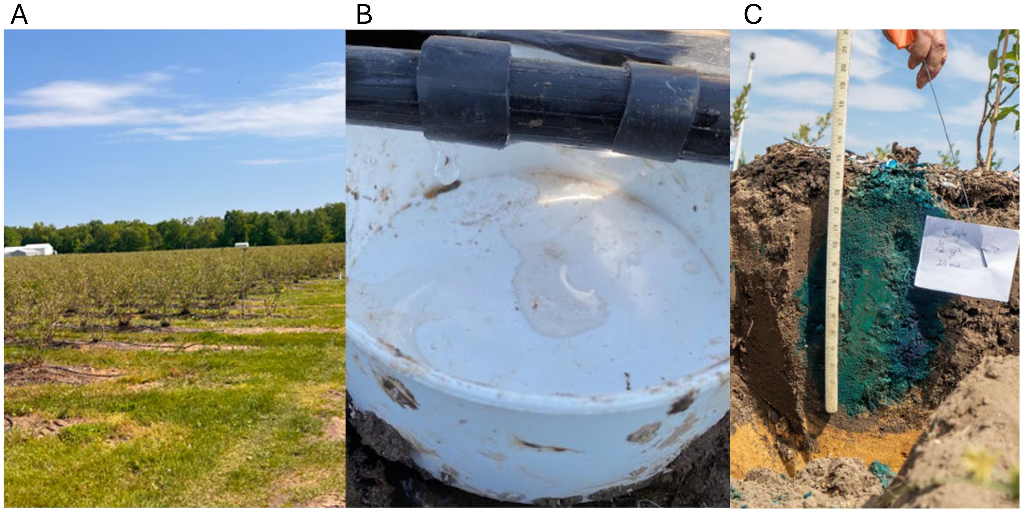
Figure 1. A commercial blueberry field in West Olive, MI, USA (A). The catch can setup to measure the water flow rate (B). A blue dye test measuring the area of the wetting region from a single emitter (C).

A Drill & Drop Bluetooth soil moisture sensor, manufactured by Sentek (Stepney, Australia), was used to monitor the change in volumetric water content at nine soil depths (0, 15, 30, 45, 60, 75, 90, 105, and 120 cm) once every hour. Sensor readings were calibrated against the gravimetric soil moisture content (Reynolds, 1970) determination to ensure accuracy. Drill & Drop soil moisture sensors were installed near the drip emitters to track the changes in soil water content throughout the 2024 growing season. Sentek sensor data were downloaded via Bluetooth monthly during the collection period and stored in the IrriMAX Live application. The Drill & Drop Sentek soil moisture readings from the 2024 growing season, May 1st–October 31st, from the depths of 15, 25, 45, and 55 cm were used for calibration, validation, and statistical analysis.

2.2 Water flow model calibration

Water flow was governed by the 2D Richard equation (Equation 1) in HYDRUS 2D:

$\begin{array}{ll}\frac{\partial \theta }{\partial t}=\frac{1}{r}\frac{\partial }{\partial r}\left[rK(h)\frac{\partial h}{\partial r}\right]+\frac{\partial }{\partial z}\left[K(h)\frac{\partial h}{\partial z}+K(h)\right]& (1)\end{array}$

where θ = volumetric water content (${\text{L}}^3{\text{L}}^{-3})$, h = soil water pressure head (L), t = time (T), r = radial space coordinate (L), z = vertical space coordinate (L), and k = hydraulic conductivity (${\text{LT}}^{-1}$).

HYDRUS 2D uses the van Genuchten Mualem (Equation 2) constitutive relationships to model the soil hydraulic properties (Equation 3) (van Genuchten, 1980):

$\begin{array}{ll}\theta (h)=\{\begin{array}{c}{\theta }_r+\frac{{\theta }_s-{\theta }_r}{{(1+{\left|\alpha h\right|}^n)}^m}, h<0\\ {\theta }_s, h\ge 0\end{array}& (2)\end{array}$

$\begin{array}{ll}K(h)=K_s{S}_e^l{\left[1-{\left(1-S_e^{\frac{1}{m}}\right)}^m\right]}^2, where, S_e=\frac{\theta -{\theta }_r}{{\theta }_s-{\theta }_r},m=1-\frac{1}{n}& (3)\end{array}$

where ${\theta }_s$ = saturated water content (${\text{L}}^3{\text{L}}^{-3}$); ${\theta }_r$ = residual water content (${\text{L}}^3{\text{L}}^{-3}$); $K_s$ = saturated hydraulic conductivity (${\text{LT}}^{-1}$); and α (${\text{L}}^{-1}$), n, and $l$ = tortuosity parameter.

For the model boundary conditions, the model used variable flux for the irrigation inflow, atmospheric boundary for precipitation and reference evapotranspiration (rET), and free drainage conditions for the outflow. The initial soil moisture content was set to field capacity (FC). In the Richards equation, soil saturated and unsaturated hydraulic conductivity functions are the main hydraulic parameters (Radcliffe and Simunek, 2010). The soil hydraulic parameters were optimized to calibrate the water flow. Soil parameters were estimated using inverse modeling. This method is commonly used in hydrologic modeling rather than direct measurement (Gupta et al., 2011). In the HYDRUS-2D model, the simulation uses an initial estimate of parameters, which were chosen as those for sandy loam soil in HYDRUS-2D, and then compares these to observed experimental data. The model then adjusted the soil hydraulic parameters to reduce the deviation between the modeled and measured soil moisture content. The simulation then uses the new parameters to run again and repeats until the modeled data closely match the measured data (Rassam et al., 2003). The calibration process entailed 50 iterations with 1,184 observations, and there were 2,032 observations for validation. The initial estimated values of hydraulic parameters were utilized from van Genuchten’s model (van Genuchten, 1980). In this study, K_s (saturated hydraulic conductivity), α (parameter in the soil water retention function), n (parameter n in the soil water retention function), and I (tortuosity parameter in the conductivity function) were optimized using the inverse function. In this study, the soil water retention curve was not directly measured in the laboratory. Instead, the retention curve parameters, such as residual water content, saturated water content, and the shape parameters of the van Genuchten–Mualem model, were estimated through inverse modeling using HYDRUS-2D. This approach involved calibrating the model using observed soil moisture data collected from the field at multiple depths and different treatments.

2.3 Statistical analysis

To evaluate the performance of HYDRUS-2D, the Nash–Sutcliffe efficiency (NSE), the index of agreement (IA), and root mean square error (RMSE) were used (Wallach, 2006; Anlauf and Rehrmann, 2013; Wegehenkel and Beyrich, 2014). NSE quantifies how the model’s simulated value is compared to the mean of the observed data. NSE is defined by (Equation 4).

$\begin{array}{ll}NSE=1-\frac{{\displaystyle {\sum }_{i=1}^N{(M_i-P_i)}^2}}{{\displaystyle {\sum }_{i=1}^N{(M_i-\overline{M})}^2}}& (4)\end{array}$

The IA is defined as the degree of model prediction error. Willmott (1981) proposed the IA, as defined by (Equation 5):

$\begin{array}{ll}IA=1-\frac{{\sum }_{i=1}^N{(M_i-P_i)}^2}{{\sum }_{i=1}^N{(\left|P_i-\overline{M}\right|+\left|M_i-\overline{M}\right|)}^2}& (5)\end{array}$

RMSE is an error index that measures the average magnitude of errors in the predicted values. RMSE is defined by (Equation 6) (Anlauf and Rehrmann, 2013):

$\begin{array}{ll}RMSE=\sqrt{\frac{1}{N}{\displaystyle {\sum }_{i=1}^N{(M_i-P_i)}^2}}& (6)\end{array}$

Where M = measured value, P = predicted value, and N = number of observations.

Defining the criteria for evaluating model performance is important. A range of recommended values was used in different studies including NSE >0 (Qiao, 2014), >0.12 (Skewes and Phogat, 2015), and >0.5 (Arora et al., 2011; Anlauf and Rehrmann, 2013). For IA, Phogat et al. (2016) and Dong et al. (2019a) reported IA >0.8 as an acceptable IA value (Skewes and Phogat, 2015; Dong et al., 2019a). For RMSE, there is a range of values reported that represent satisfactory results, and these include 0.0135 (Shekofteh et al., 2013), 0.12 (Wang et al., 2016), 0.14 (Dong et al., 2019a), and 0.03 (Ramos et al., 2012). Absolute measured error and relative error measurements were both considered to evaluate model performance (Legates and McCabe, 1999; Wegehenkel and Beyrich, 2014). This study evaluated the model calibration performance based on NSE ≥0.5, IA ≥0.8, and RMSE ≤0.030. The NSE, IA, and RMSE were calculated with Microsoft Excel software.

2.4 Flow domain and finite element mesh

Figure 2 shows the depth ranges of the three soil layers estimated by the HYDRUS-2D software. The irrigation application areas were selected as a variable flux boundary condition. Time-variable boundary conditions were used to apply irrigation at different times. Two geometry drawings were used in this study to observe two dimensions of water flow in soils. Figure 3 shows the front and side views of the soil beneath a row of blueberry plants in a typical blueberry field. The irrigation area on the boundary was identified using blue dye test results.

Figure 2

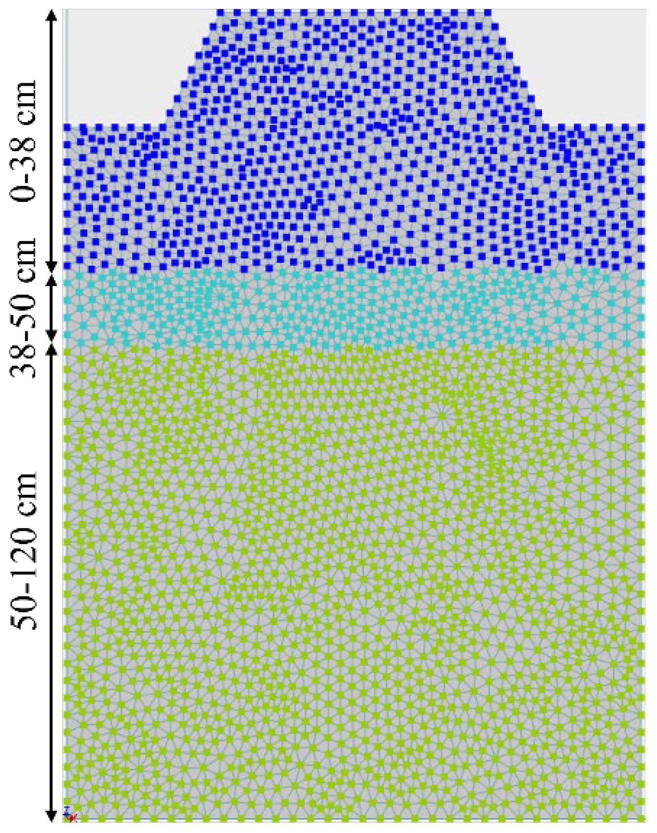
Figure 2. Depth range for three soil layers in the HYDRUS-2D model.

Figure 3

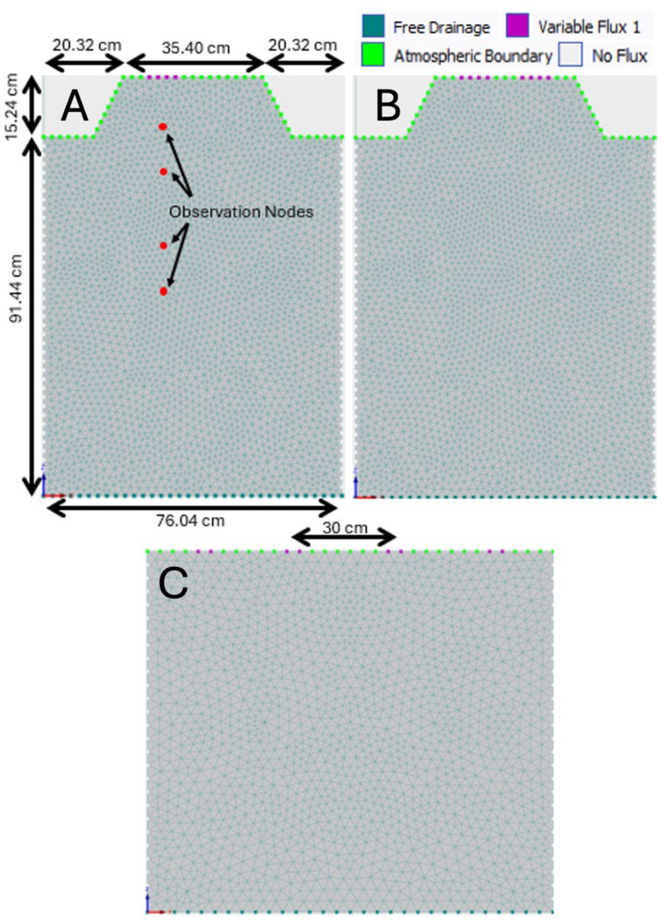
Figure 3. Flow domain and finite element mesh in HYDRUS-2D for the front view and side view of the finite element mesh for a single drip line (A), double drip line (B), and 30-cm emitter spacing (C). The observation nodes in the model coincide with the infield sensor installations at 15-, 25-, 45-, and 55-cm depths.

2.5 Simulation approach

Once the model was calibrated, HYDRUS-2D V.5 was utilized to simulate multiple drip irrigation management scenarios to maintain the optimal soil moisture levels for blueberry plants grown in sandy soils. Scenarios included evaluating 1) the irrigation application method, 2) drip irrigation spacing, 3) application duration, and 4) application rates. For the irrigation application method selection, a single drip line and a double drip line were tested to observe whether each irrigation system can adequately wet the blueberry rooting zone vertically and horizontally. Regarding the drip irrigation spacing selection, the spacing of the emitters in the drip line of 15, 30, 45, and 60 cm was evaluated. This evaluates both the water infiltration depth and width from the emitters. In addition, application duration was evaluated with the same amount of irrigation. The application durations include one full hour, half-hour, and quarter-hour applications. Moreover, two irrigation flow rates of 1.89 and 0.98 L/h and two common drip emitter flow rates used in the industry were simulated.

Different irrigation frequency efficiencies were also investigated under growing conditions in a wet year, a dry year, and an average year regarding precipitation and evapotranspiration. Hourly weather data, including precipitation and reference evapotranspiration (rET), were collected for the last 10 years, 2014–2024. The precipitation and reference ET data for the years 2014–2024 were analyzed to find the growing season with the average conditions, the highest amount of precipitation, and the lowest amount of precipitation. These were found to be the 2016 (56.03 cm), 2018 (74.46 cm), and 2021 (45.42 cm) growing seasons, respectively. Using the precipitation and reference ET values collected for these years (Figure 4), different irrigation strategies were modeled in HYDRUS-2D. These irrigation strategies all used the 1.89-L/h flow rate and 60-cm spacing, with the duration of the irrigation instance and frequency being the changing variable. Four different treatments were simulated using HYDRUS-2D: 1) irrigate for 1 h daily, 2) irrigate for 30 min daily, 3) irrigate for 30 min every other day, and 4) irrigate for 1 h once a week.

Figure 4

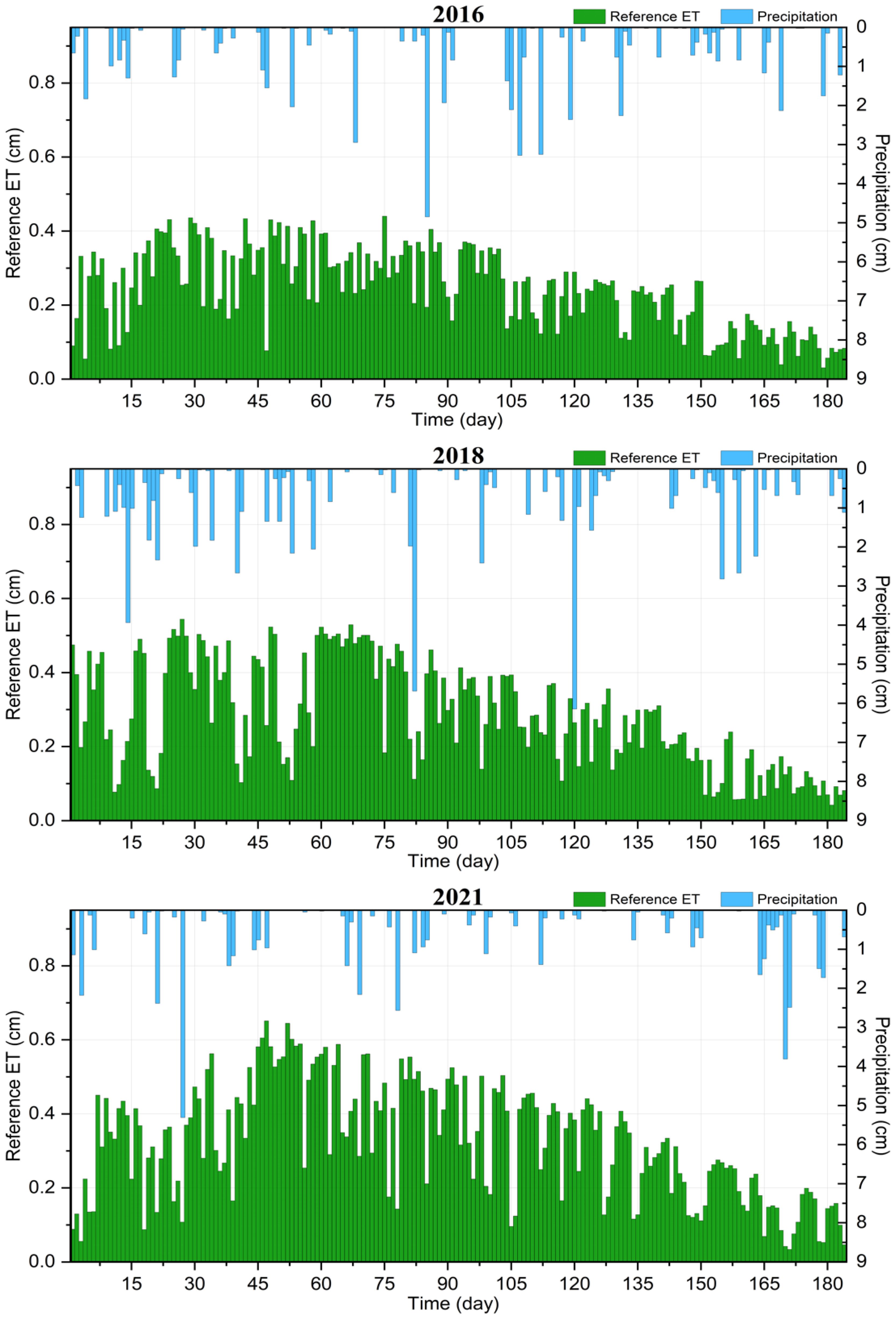
Figure 4. The value of reference ET and precipitation collected from the Michigan State University Enviroweather station in Grand Junction, MI, for the average growing season (2016), the wet season having the highest precipitation amount (2018), and the dry season having the lowest precipitation amount (2021).

3 Results

3.1 Water flow model calibration and validation

Table 1 shows the fitted values from HYDRUS-2D for hydraulic properties from the water flow calibration process for the depths defined in Figure 2. Figure 5 shows a comparison of the measurements from the soil moisture sensors and simulated soil moisture content values from HYDRUS-2D. The calibrated and validated HYDRUS model was evaluated using NSE, IA, and RMSE; these values are shown in Table 2. The modeling criteria (NSE ≥ 0.5, IA ≥ 0.8, and RMSE ≤ 0.030) were met by the output values.

Table 1

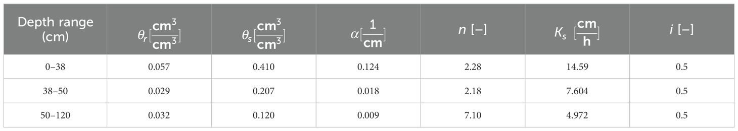
Table 1. Fitted hydraulic properties for HYDRUS water flow calibration.

Figure 5

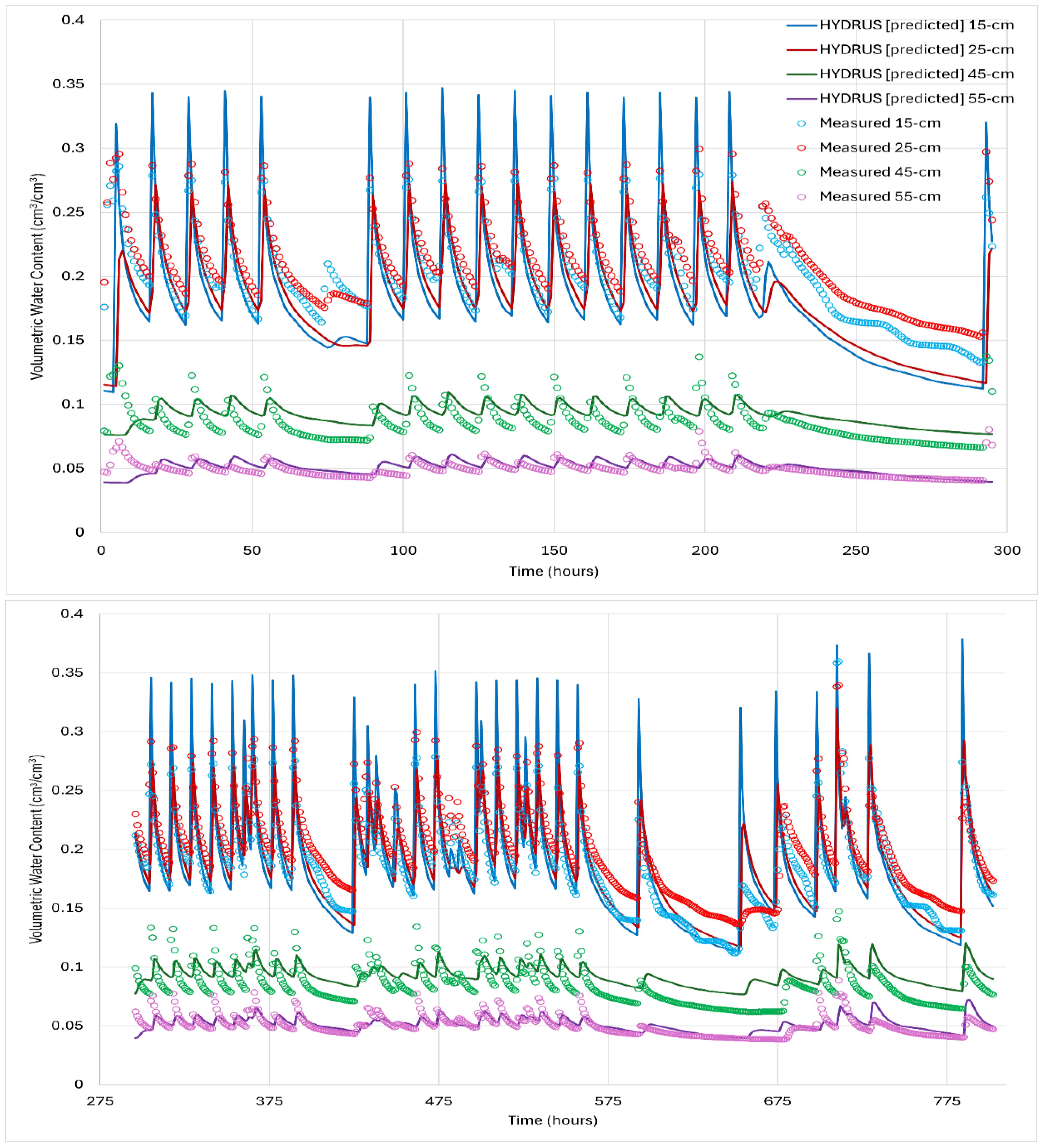
Figure 5. Comparison of the fitted HYDRUS-2D model with the measured volumetric water content from the infield sensors at 15, 25, 45, and 55 cm soil depths for calibration (top) and validation (bottom); 3,216 total data points were used for the calibration and validation process.

Table 2

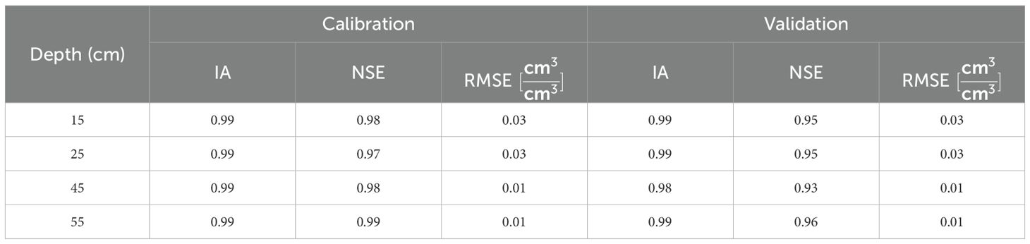
Table 2. Calculated IA, NSE, and RMSE of the calibration and validation process.

3.2 Impact of irrigation system selection

The radius of the root zone of a blueberry plant grown in sandy soil is approximately 30 cm. When using a single drip line, irrigation water adequately reached the entire width of the root zone, though a double drip line may provide a more even wetting region as it fully saturated the growing hill (Figure 6). The increasing flow rate from 0.98 to 1.89 L/h led to an increase in water content and a larger distribution around the emitters in both single and double drip lines. Regarding the infiltration depth, results indicated that a single drip line with 1.89 L/h for a half-hour application caused minimal impact on leaching water below the effective root zone. Though double drip line water application is more even, water did exceed the 30-cm depth by hours 12 and 24 for both the half- and full-hour irrigation with 1.89 L/h.

Figure 6

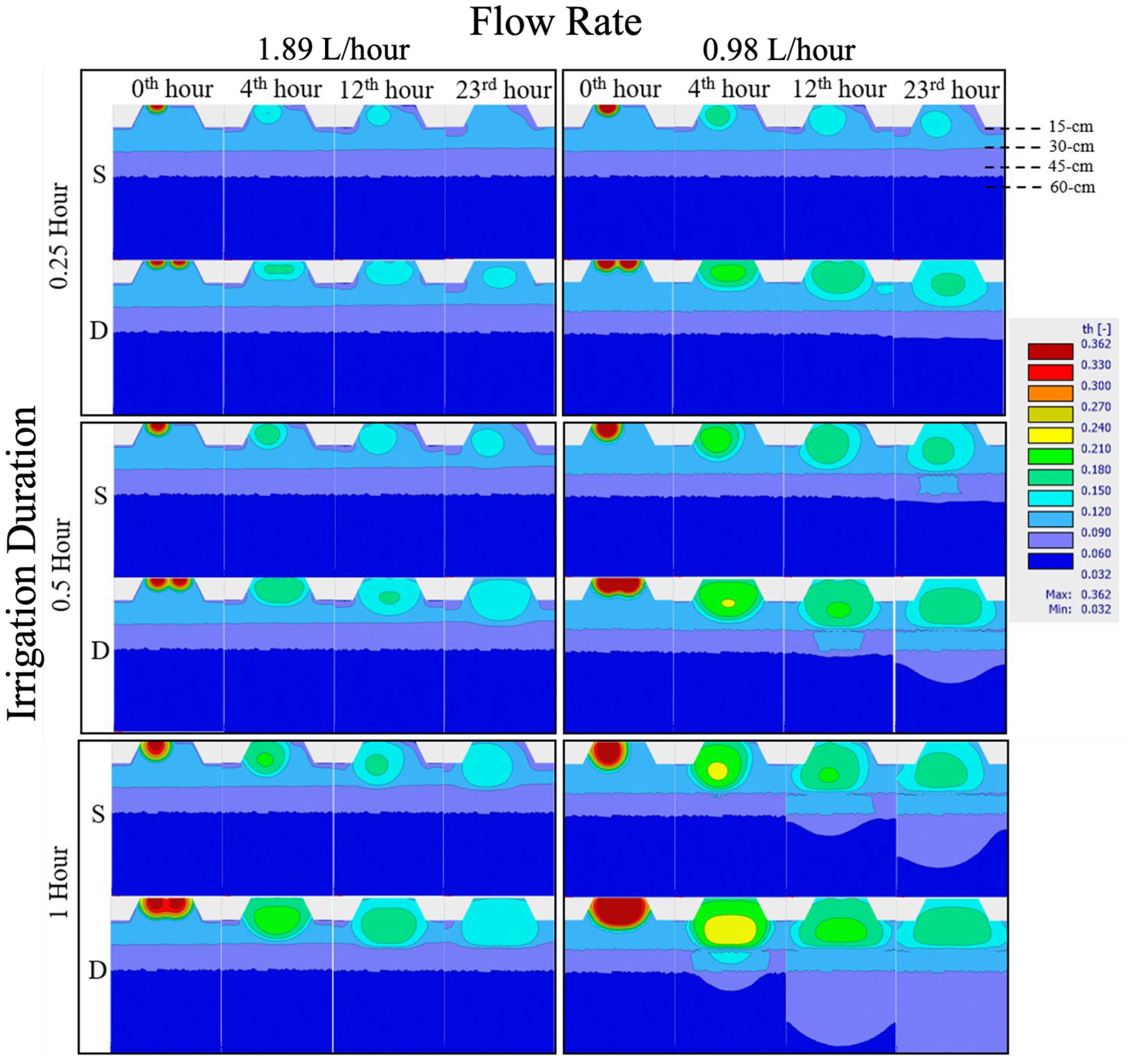
Figure 6. The effect of the drip irrigation system on coverage of the root zone after different times using different flow rates and different irrigation durations, as well as comparing single (S) and double (D) drip. The legend on the right relates color to soil moisture content.

The direction of water flow was also investigated using single and double drip lines with a flow rate of 1.89 L/h (Figure 7). With a single drip line, the movement of water can be seen evenly throughout the hill, but slower on the side without the drip. The increased amount of water from the double drip line produced water flow throughout the hill and caused faster infiltration downward. Evapotranspiration can be seen in the model with velocity vectors pointing up at the surface.

Figure 7

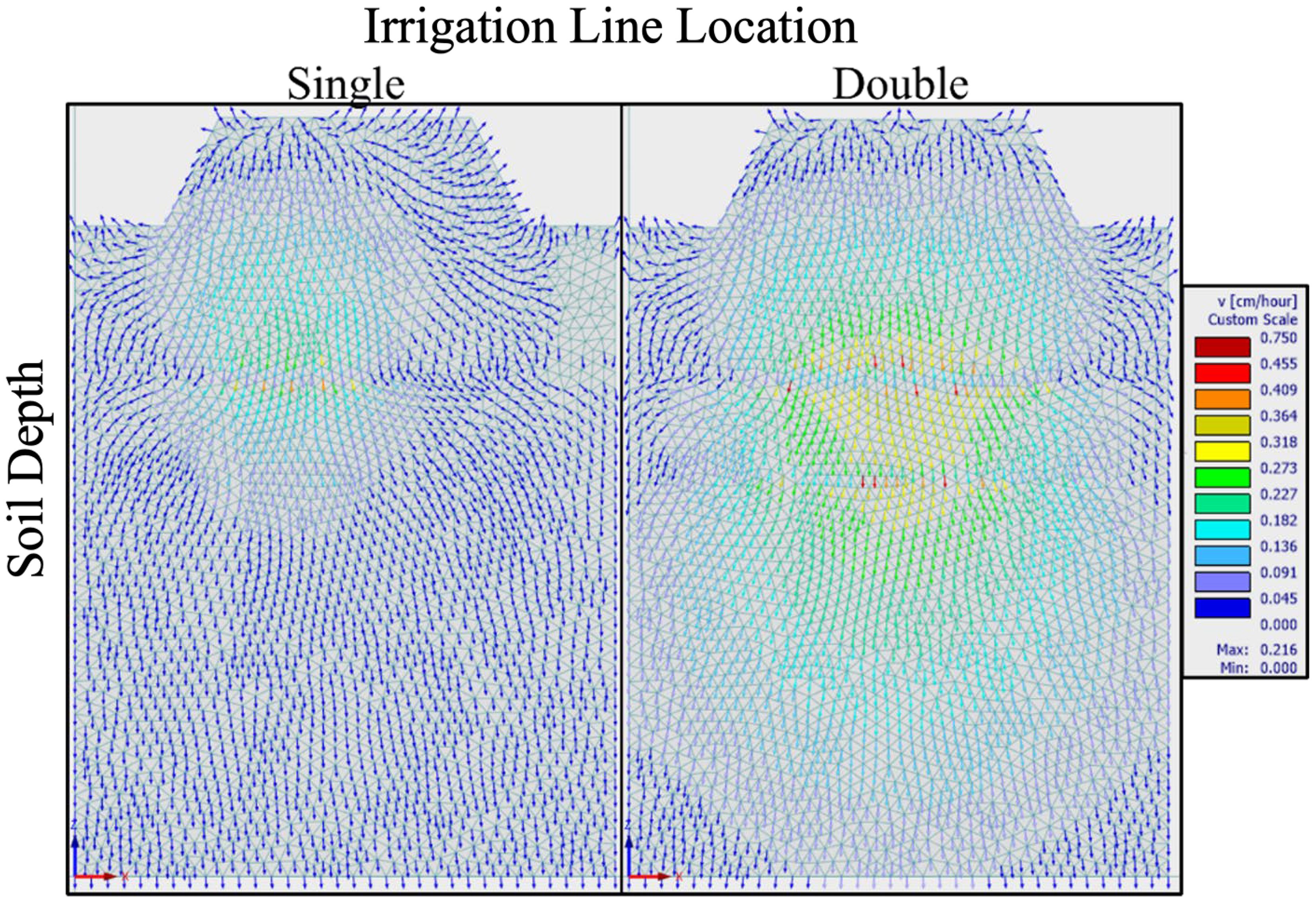
Figure 7. Comparison of the velocity vectors of water movement in a drip irrigation system with either single (left) or double (right) lines 4 h after an irrigation period of 1 h at a flow rate of 1.89 L/h. Legend on the right relating color to the velocity of water movement.

3.3 Impact of irrigation drip spacing

Drip irrigation emitter spacing of 15, 30, 45, and 60 cm was evaluated. Figure 8 shows the effect of drip emitter spacing on water flow. Water leaching past 30 cm is minimized in 45- and 60-cm emitter spacing scenarios. For 15- and 30-cm emitter spacing, the whole model was fully saturated to 120 cm after 23 h. The newer blueberry planting system places bushes 60 cm apart; thus, using a 60-cm spacing drip line, each plant will be close to an emitter. Figure 9 shows the direction and speed of water 4 h after an irrigation event using different emitter spacings. With 15-cm emitter spacing, water movement can be seen throughout the whole model, suggesting overwatering. With 45- and 60-cm emitter spacing, the direction of flow can be seen moving between the emitters to saturate the area.

Figure 8

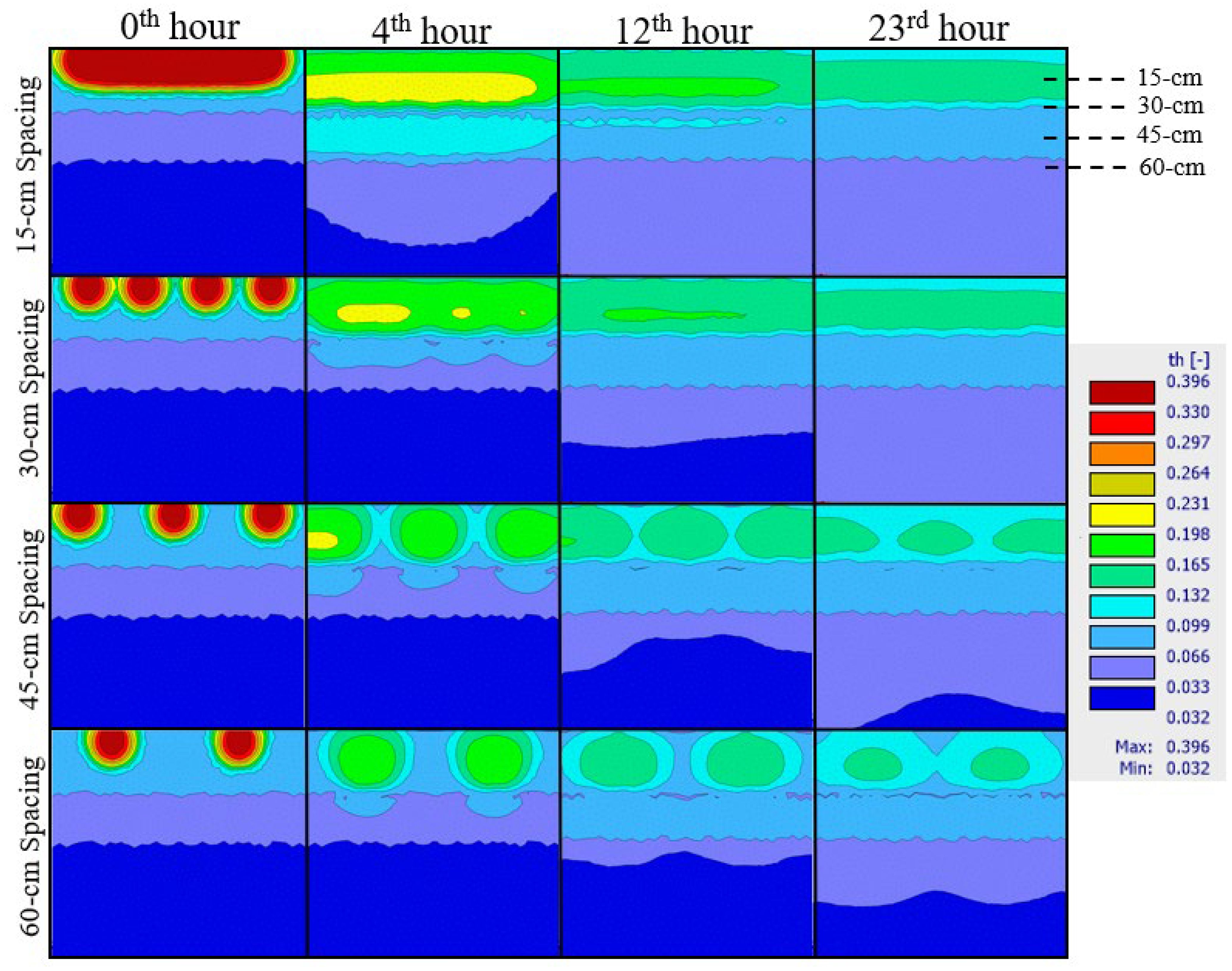
Figure 8. The HYDRUS-2D model of 1.89 L/h drip irrigation for a 1-h duration with emitter spacing at 15, 30, 45, and 60 cm on water transport in soil. The legend on the right relates color to soil moisture content.

Figure 9

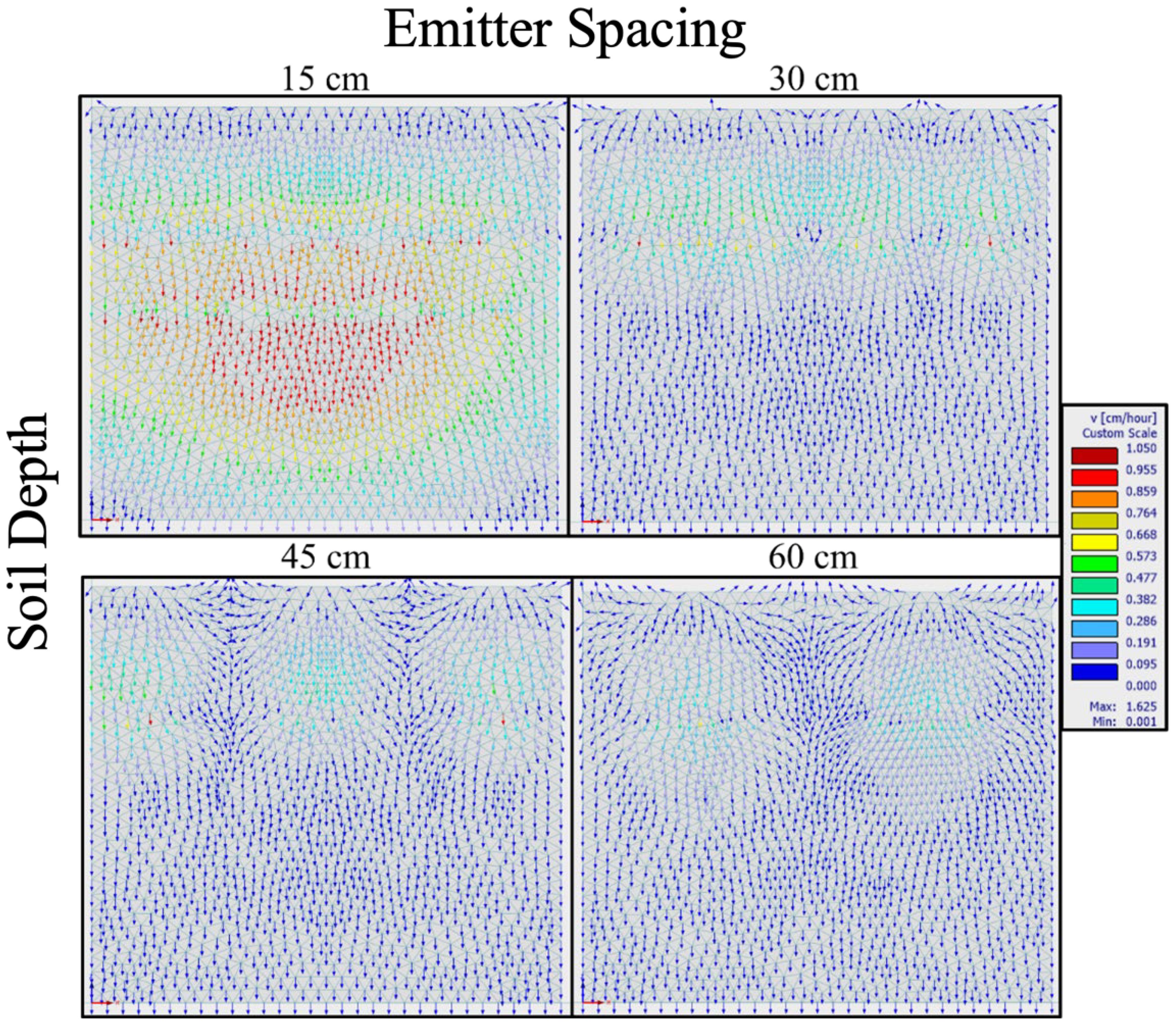
Figure 9. A comparison of the velocity vectors of water movement at 4 h after an hour duration of 1.89 L/h drip irrigation with emitter spacing of 15, 30, 45, and 60 cm. Legend on the right relating color to the velocity of water movement.

3.4 Assessment of irrigation techniques under different conditions

The change in composite soil moisture was plotted for each of the three growing seasons, under the four different irrigation treatments of interest. Each growing season was then evaluated by comparing the graphs to the FC and permanent wilting point (PWP) values. The FC and PWP were calculated for the top 60 cm of soil by assuming it to be loamy sand (Dong et al., 2020). The PWP was found to be 3.4 cm, FC to be 7.2 cm, and the recommended irrigation trigger value, at the 50% threshold, to be 5.3 cm (Figure 10). In addition, Table 3 presented the minimum, maximum, and average composite soil moisture content under each treatment of the growing season. Treatment 1 under each weather condition kept the soil moisture near or above the 50 threshold. Treatments 3 and 4 are both near the calculated PWP, being more frequent in both the dry and average years compared to the wet year, which would leave the plant under water stress. Under treatment 2, although the composite water content dips below the 50% threshold for each irrigation instance, this system does not water past or to FC, thus saving water. This treatment works best under the conditions of a wetter growing season, with the composite soil water going below the recommended irrigation point less frequently than in the other years.

Figure 10

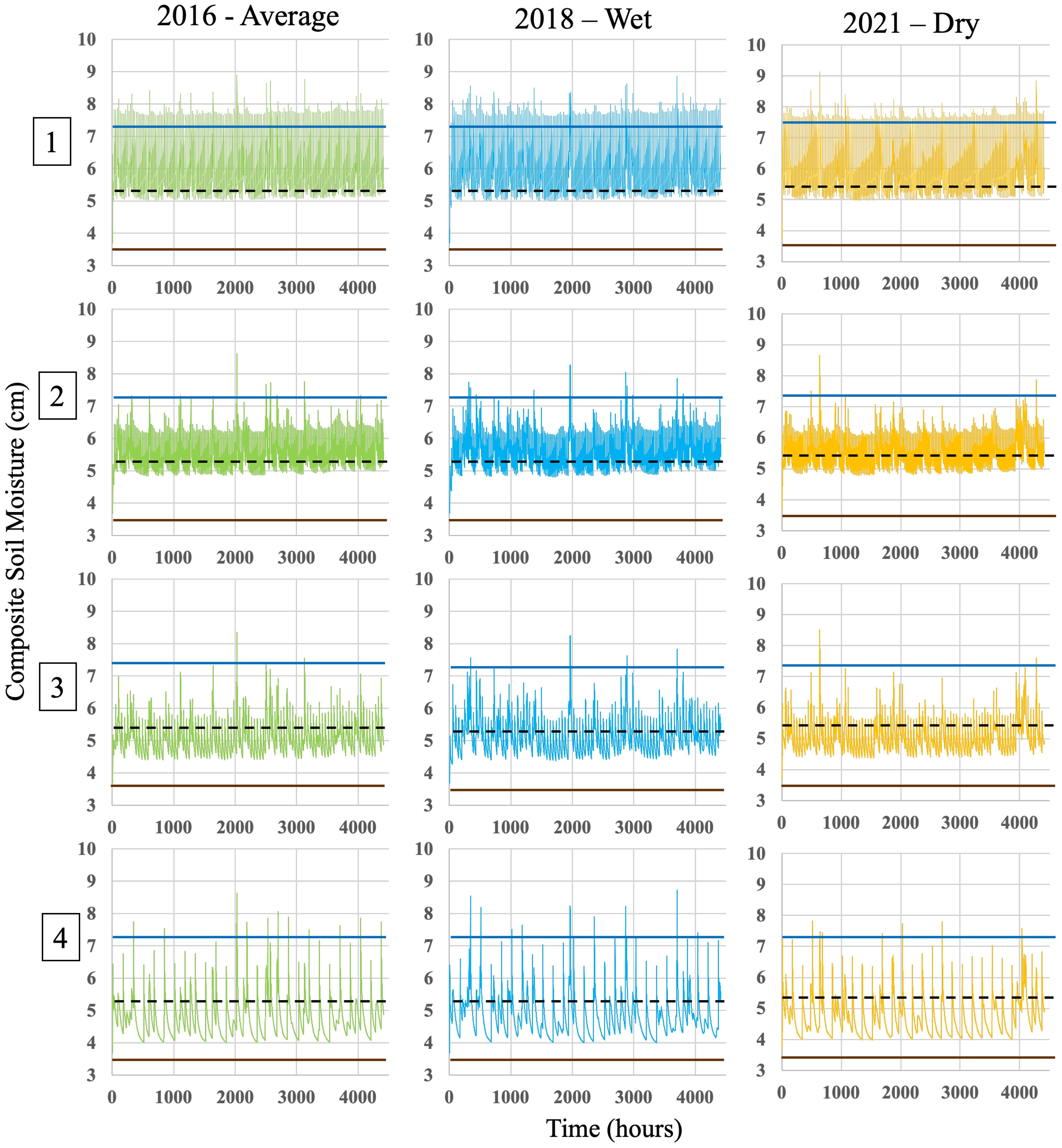
Figure 10. The change in composite soil moisture for the top 60 cm of soil throughout the average, wet, and dry growing seasons under the different irrigation treatments 1 to 4, all using a flow rate of 1.89 L/h with a 60-cm emitter spacing. The PWP (brown line), FC (dark blue line), and recommended irrigation trigger point (dashed line) are imposed on the figure. Treatment numbers are displayed on the left.

Table 3

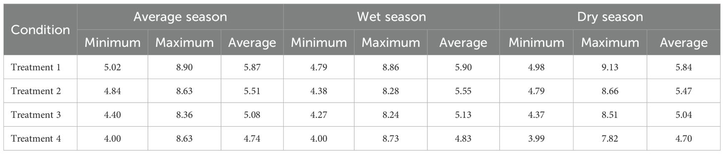
Table 3. The minimum, maximum, and average composite soil moisture content under each treatment for the duration of the growing season.

4 Discussion

4.1 Effectiveness of single and double drip irrigation arrangements

Soil moisture distribution is dependent on dripper specification and soil hydraulic parameters when using drip irrigation (Reyes-Cabrera et al., 2016). Moreover, the application efficiency is improved and the water costs are reduced when the soil moisture distribution and wetting front match the plant root distribution (Reyes-Cabrera et al., 2016). As the distance from the emitter increased, the soil moisture content decreased, with the maximum being near the emitter (Chen et al., 2025). In this study, a single-line drip irrigation system was compared with a double-line system to explore the underlying properties that govern the distribution of soil moisture. Depending on parameters such as irrigation duration and flow rate, the movement of soil moisture showed different behaviors. We observed that conditions of a single-line drip led to a consistent root zone soil moisture at all times post-irrigation event. The double-line drip supplied twice as much irrigation water compared to a single-line drip, which caused a rise in soil moisture content, but also consequently increased the loss of water from the root zone. Holzapfel et al. (2015) also reported that a blueberry orchard irrigated with two drip lines per row at a depth of 0.6 m showed a higher soil water content compared to those irrigated with four or six lines. The authors suggested that this could be due to sandy soils having a prevalence of vertical movement of water, which results in percolation losses. Wang et al. (2012) compared single and double drip line designs for cotton. The single-line design used less irrigation water, reducing water consumption. However, the double-line design improved plant emergence and increased seed cotton yield by 9%–13%. In addition, the other study was conducted to evaluate irrigation system designs under varying economic and water-saving priorities. Among the drip irrigation configurations tested, systems with double rows per lateral consistently ranked higher than single-row designs. These double-row systems were associated with lower system costs and greater water savings (Darouich et al., 2014).

Liu et al. (2012) showed that soil moisture content under a single drip tape was noticeably lower than that in a plot with double drip tape, yet no significant decrease in yield was found. This study found similar results using the single drip tape with 1.89 L/h for a half-hour. The soil moisture distribution was primarily in the range of 0–30 cm horizontally and vertically, which is proper for an effective root zone and decreases soil moisture loss compared to using similar conditions in double drip tape. In addition, in a single-line drip, the increasing flow rate from 0.98 to 1.89 L/h notably led to an increase in water content and a larger distribution around the emitters. As the wetted zone expanded, it increased the interaction between the moisture front of nearby emitters. Thus, a single drip line with the 1.89 L/h flow rate, commonly used by growers, was most efficient with a 30-min duration. However, if the drip line with 0.98 L/h is the only option, increased time of operation combined with double drip is suggested to improve application efficiency, reducing the risk of leaching below the root zone.

4.2 Impact of irrigation duration and flow rate emitter on soil water movement

In sandy soil, where water infiltrates rapidly and horizontal movement is limited, both the flow rate of the emitter and the duration of irrigation play critical roles in determining the shape and extent of the wetted zone (Nogueira et al., 2021). At a lower flow rate (0.98 L/h), water is applied slowly enough for capillary forces to act more effectively in spreading moisture horizontally. At 1.89 L/h, the higher flow rate exceeds the soil infiltration capacity at the surface, increasing gravity-driven vertical flow with limited horizontal expansion. This pattern aligns with hydraulic principles and previous findings (Vishwakarma et al., 2023b), where low flow rates in coarse soils favor surface moisture retention, while high rates promote deep movement. Several studies have indicated this relationship between flow rate and wetting pattern. For instance, Cote et al. (2003) found that decreasing flow rate from 8 to 2 L/h significantly increased the horizontal wetted diameter in loamy soils. Similarly, Li et al. (2021) reported that adjusting flow rate and the duration of drip irrigation led to considerable changes in soil moisture content at varying depths, producing a proper soil moisture distribution and increased water storage. Jia et al. (2025) found that soil texture and emitter flow rate significantly affected wetting front migration under drip irrigation. Loam showed the best upward water movement, while sandy soil favored deeper percolation, and clay restricted water flow. Optimal emitter depth and flow rate should be adjusted based on soil type to improve irrigation efficiency. Longer irrigation provides more water volume, which results in deeper wetting fronts. However, in sandy soil, low capillarity limits lateral movement, even when more water is applied.

After increasing the irrigation amount, the depth of the wetted region also increased though the width did not significantly increase. Similarly, higher flow rates and longer irrigation durations can increase the width of soil wetting. Prolonged irrigation at higher flow rates (1.89 L/h for 1 h) caused water to move rapidly beyond the root zone, resulting in deep percolation and inefficient water use. Short durations (0.25 h) may not penetrate deep enough for blueberries with 30 cm root depth, while long durations (1 h) may waste water without improving root zone coverage. Therefore, the 1.89 L/h flow rate with 0.5 h duration produced the most balanced wetting pattern reaching an adequate depth for blueberry root (30–60 cm) while minimizing vertical losses and providing some lateral moisture distribution. Previous studies have also demonstrated that the wetted zone increased both laterally and horizontally as the water supply increased (Vishwakarma et al., 2023a), and under the same flow rate and conditions, the irrigation efficiency was increased when the irrigation duration was shorter (Elmaloglou and Diamantopoulos, 2010). In addition, soil type and texture have a significant influence on the shape and size of the wetted region due to its relationship with soil properties, including water retention and hydraulic conductivity. The results showed that in sandy soil, the wetting pattern was elliptical in shape with the wetted depth larger than the wetted radius. Similarly, a study found that 94% of the applied water in sandy soils was below the emitter (Cote et al., 2003). It means water movement occurs predominantly in the vertical direction beneath the emitter. However, the wetting region was roughly spherical when in silty soil (Cote et al., 2003), and increased width in the wetted soil typically occurs with the fine-textured soils. For soils with fine texture, the average diameter and width of wetted soil were larger than coarse-textured soils (Siyal and Skaggs, 2009).

4.3 Soil moisture distribution under varying drip emitter spacing

Drip emitter spacing is one of the most influential design parameters in drip irrigation systems, directly affecting the soil moisture distribution (Bajpai and Kaushal, 2020). A major result from this study showed that the pattern of soil wetting is governed not only by emitter flow rate and irrigation duration but also by the distance between emitters along the drip line. Optimal emitter spacing ensures uniform water distribution, reduces water losses due to deep percolation, and enhances crop water use efficiency. A flow rate of 1.89 L/h with emitter spacing at 15, 30, 45, and 60 cm for 1 h influenced the distribution of soil moisture. Closer emitter spacing (15 and 30 cm) led to excessive overlaps of wetting fronts, causing significant water loss beyond the root zone. The comparative evaluation of 30- and 45-cm emitter spacings indicated that both maintained sufficient soil moisture within the effective rooting depth. However, the 45-cm emitter spacing exhibited optimal irrigation application efficiency, as it reduced the number of emitters and overall water volume, without compromising the uniformity or adequacy of moisture distribution in the root zone. Drip emitters with 60-cm spacing were spaced too widely, and unanticipated water percolation occurred as the region below the emitter may have become oversaturated. Leaching of pesticides and fertilizers can be caused by this deep percolation, leading to decreased crop production and yield (Ma et al., 2020). Similarly, the findings indicated that using an emitter spacing of 30 cm compared to 40 cm in a cotton–wheat cropping system could be more effective for increasing water productivity and yield (Yamini and Singh, 2024). Kwon et al. (2020) evaluated soil water distribution patterns between two surface drip emitters using field experiments and HYDRUS-2D simulations. Emitters were spaced at 20, 40, and 60 cm, with soil moisture measured by FDR sensors. Water content increased and saturated faster at shorter spacing (20 cm: 30–200 min) compared to wider spacing (60 cm: 900 min to over 22 h). Simulations closely matched field data (R² = 0.97). These findings help optimize drip irrigation design for improved vegetable crop productivity.

Soil texture plays a critical role in determining emitter spacing (Bajpai and Kaushal, 2020). Water infiltration of sandy soil is rapid, while lateral water movement is minimal (Faloye et al., 2025). In contrast, clay soil exhibits greater lateral water spread due to higher capillary forces, so it would be provided with wider emitter spacing without compromising moisture distribution (Vishwakarma et al., 2023a). Field experiments have further confirmed that adjusting emitter spacing based on soil texture can significantly improve water distribution uniformity and crop yield (Fattahi Nafchi et al., 2023).

4.4 Assessment of irrigation techniques under different conditions

The soil moisture distribution between FC and PWP is a critical parameter for optimizing irrigation application efficiency and maintaining favorable conditions for root water uptake, especially in shallow-rooted crops like blueberry (Bryla et al., 2011; Holzapfel et al., 2015). The results showed that longer irrigation duration (60 min daily) ensured that adequate soil moisture was attained at deeper depths. However, each irrigation event brought the soil moisture content closer to FC, even watering past this mark on several instances. Much of the water may have moved beyond the primary active root zone of blueberry, reducing irrigation application efficiency (Bwambale et al., 2022). On the other hand, the 0.5-h irrigation daily caused lower moisture but more controlled moisture distribution, keeping most of the root zone within the optimal range between FC and PWP without causing saturation or leaching (Hanson et al., 2000). The treatments of 0.5 h every other day and 1 h once a week were efficient in terms of water use and were unable to sustain soil moisture within the FC–PWP range for most of the time, leading to periodic water stress and suboptimal conditions for root water uptake (Zhang et al., 2023). In addition, the results indicate that the 0.5-h/day irrigation offered the most consistent performance across different climatic years, maintaining soil moisture within the optimal FC–PWP range and avoiding both under- and over-irrigation (Lazarovitch et al., 2023). These findings highlighted the importance of adaptive irrigation scheduling based on soil texture, crop root depth, and yearly climate variation, which can further improve irrigation application efficiency in drip-irrigated systems. In addition, future studies are recommended to incorporate a broader range of soil types as well as to integrate empirical yield data across various irrigation system designs. It would significantly improve the accuracy and practical applicability of modeling outcomes for informed irrigation management and decision-making in real-world settings.

5 Conclusion

HYDRUS-2D was successfully calibrated using the infield soil moisture sensor data. The calibrated HYDRUS model was utilized to simulate multiple scenarios to understand the impact of different irrigation design and management strategies on water flow in soil. Results showed that the best irrigation design for water flow under blueberry plants grown in sandy soil with 1.89 L/h was single drip lines for half an hour with 60-cm spacing. If a lower flow rate drip irrigation system is used, increased irrigation time or installation of a second drip line is recommended to avoid the risk of under-irrigation. Irrigation management may also need to be adjusted to the growing seasons’ weather conditions, decreasing irrigation time with higher precipitation or increasing it with higher ET. Overall, this study shows that HYDRUS-2D can be utilized as a tool to optimize the design and management practice for the drip irrigation system. As climate change has impacted agriculture, optimization of irrigation systems and practices would be important to increase the resilience of crop production to climate change.

Data availability statement

The raw data supporting the conclusions of this article will be made available by the authors, without undue reservation.

Author contributions

ST: Data curation, Investigation, Validation, Visualization, Writing – original draft, Writing – review & editing. NY: Investigation, Writing – original draft, Writing – review & editing. AR: Formal analysis, Investigation, Validation, Writing – original draft, Writing – review & editing. JV: Writing – original draft, Writing – review & editing. YD: Conceptualization, Investigation, Methodology, Project administration, Resources, Supervision, Writing – original draft, Writing – review & editing.

Funding

The author(s) declare financial support was received for the research and/or publication of this article. This work is supported by Project GREEEN, project award number GR25-013, from AgBioResearch and MSU Extension at Michigan State University, in partnership with the Michigan Department of Agriculture and Rural Development. Moreover, this project is also supported by the Michigan Blueberry Commission and the College of Agriculture and Natural Resources Undergraduate Research Program.

Acknowledgments

The authors appreciate Brenden Kelley, Carlos Garcia-Salazar, Cheyenne Sloan, Catherine Christenson, and Lyndon Kelley for their assistance with the experimental setup and data collection.

Conflict of interest

The authors declare that the research was conducted in the absence of any commercial or financial relationships that could be construed as a potential conflict of interest.

Generative AI statement

The author(s) declare that no Generative AI was used in the creation of this manuscript.

Any alternative text (alt text) provided alongside figures in this article has been generated by Frontiers with the support of artificial intelligence and reasonable efforts have been made to ensure accuracy, including review by the authors wherever possible. If you identify any issues, please contact us.

Publisher’s note

All claims expressed in this article are solely those of the authors and do not necessarily represent those of their affiliated organizations, or those of the publisher, the editors and the reviewers. Any product that may be evaluated in this article, or claim that may be made by its manufacturer, is not guaranteed or endorsed by the publisher.

References

Anlauf R. and Rehrmann P. (2013). Simulation of water and air distribution in growing media. Ed. Simunek J. (Prague, Czech Republic).

Google Scholar

Arora B., Mohanty B. P., and McGuire J. T. (2011). Inverse estimation of parameters for multidomain flow models in soil columns with different macropore densities. Water Resour Res 47, 1–17. doi: 10.1029/2010WR009451

PubMed Abstract | Crossref Full Text | Google Scholar

Bajpai A. and Kaushal A. (2020). Soil moisture distribution under trickle irrigation: A review. Water Sci. Technol. Water Supply 20, 761–772. doi: 10.2166/ws.2020.005

Crossref Full Text | Google Scholar

Bhavsar D., Limbasia B., Mori Y., Imtiyazali Aglodiya M., and Shah M. (2023). A comprehensive and systematic study in smart drip and sprinkler irrigation systems. Smart Agric. Technol 5, 100303. doi: 10.1016/J.ATECH.2023.100303

Crossref Full Text | Google Scholar

Bravdo B. and Proebsting E. L. (2018). Use of drip irrigation in orchards. Horttechnology 3, 44–49. doi: 10.21273/horttech.3.1.44

Crossref Full Text | Google Scholar

Bryla D. R., Gartung J. L., and Strik B. C. (2011). Evaluation of irrigation methods for highbush blueberry—I. Growth and water requirements of young plants. HortScience 46, 95–101. doi: 10.21273/HORTSCI.46.1.95

Crossref Full Text | Google Scholar

Bufon V. B., Lascano R. J., Bednarz C., Booker J. D., and Gitz D. C. (2012). Soil water content on drip irrigated cotton: Comparison of measured and simulated values obtained with the Hydrus 2-D model. Irrig Sci 30, 259–273. doi: 10.1007/s00271-011-0279-z

Crossref Full Text | Google Scholar

Bwambale E., Abagale F. K., and Anornu G. K. (2022). Smart irrigation monitoring and control strategies for improving water use efficiency in precision agriculture: A review. Agric. Water Manag 260, 107324. doi: 10.1016/J.AGWAT.2021.107324

Crossref Full Text | Google Scholar

Chen R., Filipović V., Zhang J., Li W., Ye H., Zhang J., et al. (2025). Uncovering soil preferential flow induced by different drip irrigation emitter settings: Insights integrating wetting-fronts image variability, HYDRUS-2D, and active region model. Catena (Amst) 249, 108669. doi: 10.1016/J.CATENA.2024.108669

Crossref Full Text | Google Scholar

Cordel J., Anlauf R., Pramabing W., and Broll G. (2025). Predicting water distribution and optimizing irrigation management in turfgrass rootzones using HYDRUS-2. Hydrology 12, 53. doi: 10.3390/hydrology12030053

Crossref Full Text | Google Scholar

Cote C. M., Bristow K. L., Charlesworth P. B., Cook F. J., and Thorburn P. J. (2003). Analysis of soil wetting and solute transport in subsurface trickle irrigation. Irrig Sci 22, 143–156. doi: 10.1007/s00271-003-0080-8

Crossref Full Text | Google Scholar

Darouich H. M., Pedras C. M. G., Gonçalves J. M., and Pereira L. S. (2014). Drip vs. surface irrigation: A comparison focussing on water saving and economic returns using multicriteria analysis applied to cotton. Biosyst. Eng 122, 74–90. doi: 10.1016/J.BIOSYSTEMSENG.2014.03.010

Crossref Full Text | Google Scholar

Dong Y. (2022). “Irrigation scheduling methods: overview and recent advances,” in Irrigation and Drainage - Recent Advances (IntechOpen). doi: 10.5772/intechopen.107386

Crossref Full Text | Google Scholar

Dong Y., Christenson C., Kelley L., and Miller S. (2024). Trends and future of agricultural irrigation in Michigan and Indiana. Irrigation Drainage 73, 346–358. doi: 10.1002/ird.2862

Crossref Full Text | Google Scholar

Dong Y., Miller S., and Kelley L. (2020). Improving Irrigation Water Use Efficiency: Using Soil Moisture Sensors. Available online at: https://www.egr.msu.edu/bae/water/irrigation/sites/default/files/content/E3445_ImprovingIrrigationWaterUse.pdf (Accessed July 10, 2020).

Google Scholar

Dong Y., Safferman S. I., and Nejadhashemi A. P. (2019a). Land-based wastewater treatment system modeling using HYDRUS CW2D to simulate the fate, transport, and transformation of soil contaminants. J. Sustain Water Built Environ 5, 1–9. doi: 10.1061/jswbay.0000890

Crossref Full Text | Google Scholar

Dong Y., Safferman S. I., and Pouyan Nejadhashemi A. (2019b). Computational modeling of wastewater land application treatment systems to determine strategies to improve carbon and nitrogen removal. J. Environ. Sci. Health A Tox Hazard Subst Environ. Eng 54, 657–667. doi: 10.1080/10934529.2019.1579536

PubMed Abstract | Crossref Full Text | Google Scholar

Egea G., Muñiz J., and Diaz-Espejo A. (2017). Optimization of an automatic irrigation system for precision irrigation of blueberries grown in sandy soil. Adv. Anim. Biosci 8, 551–556. doi: 10.1017/s204047001700005x

Crossref Full Text | Google Scholar

Elmaloglou S. and Diamantopoulos E. (2010). Soil water dynamics under surface trickle irrigation as affected by soil hydraulic properties, discharge rate, dripper spacing and irrigation duration. Irrigation Drainage 59, 254–263. doi: 10.1002/ird.471

Crossref Full Text | Google Scholar

Elnesr M. N. and Alazba A. A. (2019). Computational evaluations of HYDRUS simulations of drip irrigation in 2D and 3D domains (i-Surface drippers). Comput. Electron Agric 162, 189–205. doi: 10.1016/j.compag.2019.03.035

Crossref Full Text | Google Scholar

Faloye O. T., Ezeh A., Kamchoom V., Abioye O. M., and Ikubanni P. P. (2025). Development of soil wetting front estimation models in sandy soil with a hard pan under drip irrigation using empirical and response surface methodologies. Agronomy 15, 1–19. doi: 10.3390/agronomy15020272

Crossref Full Text | Google Scholar

Fattahi Nafchi R., Valiyari-Eskandari M., Raeisi Vanani H., Ostad-Ali-Askari K., and Bahrami A. (2023). Evaluation of wetting front detector to estimate the dimensions of wetting front in the drip irrigation. J. Eng. Appl. Sci 70, 1–9. doi: 10.1186/s44147-023-00295-5

Crossref Full Text | Google Scholar

Feng Z., Miao Q., Shi H., Li X., Yan J., Gonçalves J. M., et al. (2024). Irrigation scheduling in sand-layered farmland: Evaluation of water and salinity dynamics in the soil by SALTMED-1D model under mulched maize production in Hetao Irrigation District, China. Eur. J. Agron 157, 127177. doi: 10.1016/J.EJA.2024.127177

Crossref Full Text | Google Scholar

Goldy R. (2012). Soil type influences irrigation strategy. MI, United States: Michigan State Univ. Extension. Available online at: https://www.canr.msu.edu/news/soil_type_influences_irrigation_stategy.

Google Scholar

Gupta H. V., Sorooshian S., Hogue T. S., and Boyle D. P. (2011). Advances in automatic calibration of watershed models. Washington, D.C, USA: American Geophysical Union (AGU), 9–22. doi: 10.1029/ws006p0009

Crossref Full Text | Google Scholar

Hanson B. R., Orloff S., and Peters D. (2000). Monitoring soil moisture helps refine irrigation management. Calif Agric. (Berkeley) 54, 38–42. doi: 10.3733/ca.v054n03p38

Crossref Full Text | Google Scholar

Holzapfel E., Jara J., and Coronata A. M. (2015). Number of drip laterals and irrigation frequency on yield and exportable fruit size of highbush blueberry grown in a sandy soil. Agric. Water Manag 148, 207–212. doi: 10.1016/J.AGWAT.2014.10.001

Crossref Full Text | Google Scholar

Honari M., Ashrafzadeh A., Khaledian M., Vazifedoust M., and Mailhol J. C. (2017). Comparison of HYDRUS-3D soil moisture simulations of subsurface drip irrigation with experimental observations in the South of France. J. Irrigation Drainage Eng 143, 04017014. doi: 10.1061/(asce)ir.1943-4774.0001188

Crossref Full Text | Google Scholar

Jia M. L., Wei S., Liu F., Zhang Y. C., and Shen Y. J. (2025). Influence of soil texture and drip emitter flow rate on soil water movement under subsurface drip irrigation. Chin. J. Eco-Agriculture. 33 (4), 749–758. doi: 10.12357/cjea.20240081

Crossref Full Text | Google Scholar

Kandelous M. M. and Šimůnek J. (2010). Numerical simulations of water movement in a subsurface drip irrigation system under field and laboratory conditions using HYDRUS-2D. Agric. Water Manag 97, 1070–1076. doi: 10.1016/j.agwat.2010.02.012

Crossref Full Text | Google Scholar

Kovach M. (2006). A Statistical Analysis of the Distribution of Roads Salt in Blueberry Farm Soils of Van Buren County, Michigan (Western Michigan University).

Google Scholar

Kwon S. H., Kim D. H., Kim J. S., Jung K. Y., Lee S. H., and Kwon J. K. (2020). Soil water flow patterns due to distance of two emitters of surface drip irrigation for horticultural crops. Hortic. Sci. Technol 38, 631–644. doi: 10.7235/HORT.20200058

Crossref Full Text | Google Scholar

Lamm F. R. and Trooien T. P. (2003). Subsurface drip irrigation for corn production: A review of 10 years of research in Kansas. Irrig Sci 22, 195–200. doi: 10.1007/s00271-003-0085-3

Crossref Full Text | Google Scholar

Lazarovitch N., Kisekka I., Oker T. E., Brunetti G., Wöhling T., Xianyue L., et al. (2023). Modeling of irrigation and related processes with HYDRUS. Adv. Agron 181, 79–181. doi: 10.1016/BS.AGRON.2023.05.002

Crossref Full Text | Google Scholar

Legates D. R. and McCabe G. J. (1999). Evaluating the use of “goodness-of-fit” measures in hydrologic and hydroclimatic model validation. Water Resour Res 35, 233–241. doi: 10.1029/1998WR900018

Crossref Full Text | Google Scholar

Li Y., Yu Q., Ning H., Gao Y., and Sun J. (2023). Simulation of soil water, heat, and salt adsorptive transport under film mulched drip irrigation in an arid saline-alkali area using HYDRUS-2D. Agric. Water Manag 290, 108585. doi: 10.1016/j.agwat.2023.108585

Crossref Full Text | Google Scholar

Li Z., Zong R., Wang T., Wang Z., and Zhang J. (2021). Adapting root distribution and improving water use efficiency via drip irrigation in a jujube (Zizyphus jujube mill.) orchard after long-term flood irrigation. Agric. (Switzerland) 11, 1184. doi: 10.3390/agriculture11121184

Crossref Full Text | Google Scholar

Liang S., Abd El Baki H. M., An P., and Fujimaki H. (2022). Determining irrigation volumes for enhancing profit and N uptake efficiency of potato using WASH_2D model. Agronomy 12, 2372. doi: 10.3390/agronomy12102372

Crossref Full Text | Google Scholar

Liu M. X., Yang J. S., Li X. M., Yu M., and Wang J. (2012). Effects of irrigation water quality and drip tape arrangement on soil salinity, soil moisture distribution, and cotton yield (Gossypium hirsutum L.) under mulched drip irrigation in Xinjiang, China. J. Integr. Agric 11, 502–511. doi: 10.1016/S2095-3119(12)60036-7

Crossref Full Text | Google Scholar

Ma C., Xiao Y., Puig-Bargués J., Shukla M. K., Tang X., Hou P., et al. (2020). Using phosphate fertilizer to reduce emitter clogging of drip fertigation systems with high salinity water. J. Environ. Manage 263, 110366. doi: 10.1016/J.JENVMAN.2020.110366

PubMed Abstract | Crossref Full Text | Google Scholar

Moursi H., Youssef M. A., and Chescheir G. M. (2022). Development and application of DRAINMOD model for simulating crop yield and water conservation benefits of drainage water recycling. Agric. Water Manag 266, 107592. doi: 10.1016/J.AGWAT.2022.107592

Crossref Full Text | Google Scholar

Nogueira V. H. B., Diotto A. V., Thebaldi M. S., Colombo A., Silva Y. F., Lima E. M., et al. (2021). Variation in the flow rate of drip emitters in a subsurface irrigation system for different soil types. Agric. Water Manag 243, 106485. doi: 10.1016/J.AGWAT.2020.106485

Crossref Full Text | Google Scholar

Phogat V., Skewes M. A., Cox J. W., and Simunek J. (2016). Statistical assessment of a numerical model simulating agro hydro-chemical processes in soil under drip fertigated mandarin tree. Irrigation Drainage Syst. Eng. 5 (1), 1–9. doi: 10.4172/2168-9768.1000155

Crossref Full Text | Google Scholar

Puertes C., Lidón A., Echeverría C., Bautista I., González-Sanchis M., del Campo A. D., et al. (2019). Explaining the hydrological behaviour of facultative phreatophytes using a multi-variable and multi-objective modelling approach. J. Hydrol (Amst) 575, 395–407. doi: 10.1016/J.JHYDROL.2019.05.041

Crossref Full Text | Google Scholar

Qiao S. Y. (2014). Modeling water flow and phosphorus fate and transport in a tile-drained clay loam soil using HYDRUS (2D/3D) (McGill University).

Google Scholar

Radcliffe D. and Simunek J. (2010). Soil Physics with HYDRUS: Modeling and Applications (Boca Raton, FL: Taylor & Francis Group).

Google Scholar

Ramos T. B., Šimůnek J., Gonçalves M. C., Martins J. C., Prazeres A., and Pereira L. S. (2012). Two-dimensional modeling of water and nitrogen fate from sweet sorghum irrigated with fresh and blended saline waters. Agric. Water Manag 111, 87–104. doi: 10.1016/j.agwat.2012.05.007

Crossref Full Text | Google Scholar

Rassam D., Simunek J., and van Geuchten M. (2003). Modelling Variably Saturated Flow with HYDRUS-2D (Brisbane, Australia: ND Consult).

Google Scholar

Reyes-Cabrera J., Zotarelli L., Dukes M. D., Rowland D. L., and Sargent S. A. (2016). Soil moisture distribution under drip irrigation and seepage for potato production. Agric. Water Manag 169, 183–192. doi: 10.1016/J.AGWAT.2016.03.001

Crossref Full Text | Google Scholar

Reynolds S. G. (1970). The gravimetric method of soil moisture determination Part I A study of equipment, and methodological problems. J. Hydrol (Amst) 11, 258–273. doi: 10.1016/0022-1694(70)90066-1

Crossref Full Text | Google Scholar

Shekofteh H., Afyuni M., Hajabbasi M. A., Iversen B. V., Nezamabadi-Pour H., Abassi F., et al. (2013). Modeling of nitrate leaching from a potato field using HYDRUS-2D. Commun. Soil Sci. Plant Anal 44, 1–15. doi: 10.1080/00103624.2013.829082

Crossref Full Text | Google Scholar

Simonne E., Studstill D., Dukes M., Duval J., Hochmuth R., Mcavoy G., et al. (2004). How to Conduct an On-farm Dye Test and Use the Results to Improve Drip Irrigation Management in Vegetable Production 1. Available online at: http://nfrec-sv.ifas.ufl.edu/ (Accessed October 28, 2025).

Google Scholar

Siyal A. A. and Skaggs T. H. (2009). Measured and simulated soil wetting patterns under porous clay pipe sub-surface irrigation. Agric. Water Manag 96, 893–904. doi: 10.1016/J.AGWAT.2008.11.013

Crossref Full Text | Google Scholar

Skaggs T. H., Trout T. J., Simunek J., and Shouse P. J. (2004). Comparison of HYDRUS-2D simulations of drip irrigation with experimental observations. J. Irrigation Drainage Eng 130, 304–310. doi: 10.1061/(ASCE)0733-9437(2004)130:4(304)

Crossref Full Text | Google Scholar

Skewes M. A. and Phogat V. (2015). Statistical assessment of a numerical model simulating agro hydrochemical processes in soil under drip fertigated mandarin tree. Irrigation Drainage Syst. Eng 05, 1000155. doi: 10.4172/2168-9768.1000155

Crossref Full Text | Google Scholar

Surendran U. and Madhava Chandran K. (2022). Development and evaluation of drip irrigation and fertigation scheduling to improve water productivity and sustainable crop production using HYDRUS. Agric. Water Manag 269, 107668. doi: 10.1016/j.agwat.2022.107668

Crossref Full Text | Google Scholar

USDA-NASS (2023). Noncitrus Fruits and Nuts. 2015–2022 Summary (USDA National Agricultural Statistical Service (USDA-NASS)). Available online at: https://usda.library.cornell.edu/concern/publications/zs25x846c (Accessed August 6, 2025).

Google Scholar

van Dam J. C., Groenendijk P., Hendriks R. F. A., and Kroes J. G. (2008). Advances of modeling water flow in variably saturated soils with SWAP. Vadose Zone J 7, 640–653. doi: 10.2136/vzj2007.0060

Crossref Full Text | Google Scholar

van Genuchten M. (1980). A closed-form equation for predicting the hydraulic conductivity of unsaturated soils. Soil Sci. Soc. America J 44, 892–898. doi: 10.2136/sssaj1980.03615995004400050002x

Crossref Full Text | Google Scholar

Vishwakarma, Al-Ansari, Kumar A., Kushwaha N. L., Yadav D., Kumawat A., et al. (2023a). Modeling of soil moisture movement and wetting behavior under point-source trickle irrigation. Sci. Rep 13, 14981. doi: 10.1038/s41598-023-41435-4. N.

PubMed Abstract | Crossref Full Text | Google Scholar

Vishwakarma D. K., Kumar R., Tomar A. S., and Kuriqi A. (2023b). Eco-hydrological modeling of soil wetting pattern dimensions under drip irrigation systems. Heliyon 9, e18078. doi: 10.1016/J.HELIYON.2023.E18078

PubMed Abstract | Crossref Full Text | Google Scholar

Wallach D. (2006). Evaluating Crop Models. Ed. Wallach D. (New York: Elsevier).

Google Scholar

Wang J., Bai Z., and Yang P. (2016). Using HYDRUS to simulate the dynamic changes of ca2+ and na+ in sodic soils reclaimed by gypsum. Soil Water Res 11, 1–10. doi: 10.17221/14/2015-SWR

Crossref Full Text | Google Scholar

Wang R. S., Wan S. Q., Kang Y. H., and Liu S. P. (2012). Comparison of two dripper line designs to assess cotton yield, water use, and net return in Northwest China. J. Integr. Agric 11, 1924–1932. doi: 10.1016/S2095-3119(12)60198-1

Crossref Full Text | Google Scholar

Wegehenkel M. and Beyrich F. (2014). Modelling hourly evapotranspiration and soil water content at the grass-covered boundary-layer field site Falkenberg, Germany. Hydrological Sci. J 59, 376–394. doi: 10.1080/02626667.2013.835488

Crossref Full Text | Google Scholar

Willmott C. J. (1981). On the validation of models. Phys. Geogr. 2 (2), 184–194. doi: 10.1080/02723646.1981.10642213

Crossref Full Text | Google Scholar

Yamini V. and Singh K. (2024). Emitter spacing, depth of lateral placement, and nutrient levels affect productivity of cotton-wheat cropping system under sub-surface drip fertigation. Agric. Water Manag 295, 108761. doi: 10.1016/J.AGWAT.2024.108761

Crossref Full Text | Google Scholar

Zhang Y., Li X., Šimůnek J., Shi H., Chen N., and Hu Q. (2023). Quantifying water and salt movement in a soil-plant system of a corn field using HYDRUS (2D/3D) and the stable isotope method. Agric. Water Manag 288, 108492. doi: 10.1016/J.AGWAT.2023.108492

Crossref Full Text | Google Scholar