Integrating weather variables and AI models for forecasting major pests in jute: applications in climate-smart crop management

Jute crop suffers a substantial amount of physical and economic loss every year due to the infestation of several insect pests, such as yellow mite (Polyphagotarsonemus latus Banks) and jute semilooper (Anomis sabulifera Guen), at different stages of crop growth. This study utilizes data on the mean incidence of yellow mite and jute semilooper at different days after sowing (DAS) from 2013 to 2023, along with weather variables, collected at the AINP-JAF, UBKV Centre, Cooch Behar, West Bengal. The results indicate that the incidence of jute semilooper follows a seasonal pattern, with most peaks occurring at approximately 45 DAS. Additionally, the mean incidence of yellow mite is found to be significantly positively correlated with maximum temperature and negatively correlated with minimum and maximum relative humidity at a 2-week lag. This suggests that dry weather with high temperatures 2 weeks prior contributes to higher yellow mite infestations at the current time. A similar correlation is observed for jute semilooper infestation. Various time series and machine learning models, including Autoregressive Integrated Moving Average (ARIMA), ARIMA-T, Seasonal ARIMA (SARIMA), SARIMA-T, ARIMA with exogenous variables (ARIMAX), SARIMA with exogenous variables (SARIMAX)-T, Random Forest, Support Vector Regression (SVR), and TDNNX, are applied to the training dataset from 2013 to 2022. The models are validated using the test data for the year 2023, based on root mean square error (RMSE) and root median square error (RMdSE) values. For yellow mite, TDNNX is found to be the best fitted model followed by SVR and SARIMAX-T in terms of RMSE and RMdSE values. Similarly, for jute semilooper, TDNNX is found to be the best fitted model followed by Random Forest and SARIMA. Finally, pest incidence forecasts for yellow mite and jute semilooper are obtained for 2024 using the forecasted and average weather data, applying the TDNNX model.

Introduction

Jute, a cost-effective natural fiber, ranks second only to cotton in terms of production and versatility. In India, jute farming covers 646.11 thousand hectares, yielding 94.49 lakh tons with a productivity of 2.62 tons per hectare in 2023–2024 (Directorate of Economics and Statistics, MoAFW, Govt. of India). The raw jute sector provides significant employment to the rural population due to its labor-intensive nature. West Bengal, which accounts for 78.94% of the cultivated jute land and 82% of the production, is the leading jute-growing state in India. The sector holds social, economic, and physical value for approximately 33–35 lakh small and marginal farmers in India (Sarkar and Majumdar, 2016). In 2023–2024, West Bengal cultivated 6.46 lakh hectares of jute, producing 94.49 lakh bales (Directorate of Economics and Statistics, MoAFW, Govt. of India). Cooch Behar is one of the major districts in the state for jute fiber cultivation.

Jute is an essential cash crop for farmers, but challenges such as pest infestations and pricing issues hinder its growth. Oversupply in the market and the scarcity of high-yielding seeds restrict the farmers’ ability to adopt advanced technologies, reducing their interest in high-yielding jute varieties (Hussain et al., 2002). Jute cultivation, typically carried out during the pre-kharif season, suffers significant physical and economic losses each year due to infestations by major insect pests like yellow mite (Polyphagotarsonemus latus Banks) and jute semilooper (Anomis sabulifera Guen) at various stages of crop growth. In West Bengal, the avoidable loss in fiber yield has been estimated to range from 31% to 34% (Rahman and Khan, 2012). These losses could be minimized through sustainable plant protection measures, such as integrated pest management, biological control, and mechanical methods.

Timely and accurate forecasting of pest incidence using mathematical, statistical, and simulation models can help minimize these losses by enabling farmers to implement appropriate pest management strategies. With the advancement of computing power, machine learning models are increasingly used for precise forecasting (Durgabai and Bhargavi, 2018). Numerous studies have shown that weather variables—particularly temperature, relative humidity, and rainfall—play a crucial role in the occurrence and survival of various insect pests on jute crops (Rahman and Khan, 2012; Suyal et al., 2018). It has also been found that pest incidence is correlated with both the current time period and lead times ranging from 1 to 4 weeks (Katke et al., 2009; Balikai and Venkatesh, 2019). Therefore, incorporating weather variables along with past pest incidence data provides a solid foundation for developing reliable pest prediction models. Several researchers have already developed weather-based models for predicting crop pests and diseases (Sarkar et al., 2023; Vaidheki et al., 2023). Therefore, in the present study, an attempt has been made to forecast the mean incidence of major pests of jute crop in Cooch Behar district of West Bengal using machine learning models and weather data.

Materials and methods

Description of data

The incidence data of major jute pests used in this study are secondary data obtained from the All India Network Project (AINP) on Jute and Allied Fibers, Uttar Banga Krishi Viswavidyalaya (UBKV) Centre, Pundibari, Cooch Behar, West Bengal, covering the period from 2013 to 2023. During each crop season, yellow mite and jute semilooper incidences are available at 25, 35, 45, 55, 65, and 75 days after sowing (DAS). The infestation level of the semilooper is measured as the percentage of infestation, while yellow mite incidence is quantified by counting its number per square centimeter on the second unfold leaf. The pest incidence data used in this study were collected from control fields, i.e., without pest control operations, from a widely cultivated variety of jute, JRO-524 recommended for the region. The same variety was consistently used across all years of the study (2013–2023) to maintain uniformity in pest incidence data collection and avoid variability arising from genetic differences among varieties. It was consistently observed across all years that pest incidence at 25 and 75 DAS was zero. Including these zero values in the analysis could lead to inconsistencies in model fitting and forecasting. Moreover, the study focuses primarily on pest incidences that exceed the economic threshold levels—approximately five mites per square centimeter for yellow mite and 10% infestation for jute semilooper, as reported in the literature. Therefore, data from 25 and 75 DAS were excluded, and the analysis was conducted using the remaining data points where significant pest incidence was observed. Similarly, the weather data used in this study are secondary data obtained from the records of Gramin Krishi Mausam Sewa (GKMS), Agrometeorological Field Unit (AMFU), Pundibari, UBKV. The dataset includes daily observations of rainfall (mm), maximum and minimum temperatures (MaxT and MinT in °C), and maximum and minimum relative humidity (MaxRH and MinRH in %) spanning the period from 2013 to 2023. These daily records were aggregated into weekly data based on the Standard Meteorological Weeks (SMWs) to correspond with the pest incidence survey dates. For each SMW, the rainfall values were summed, while the temperature and relative humidity variables were averaged to ensure consistency with the timing of pest observations.

Methodology

To check the presence of seasonality in pest incidence, time plots of the mean incidence of both pests are constructed along with the Webel–Ollech (WO) seasonality test. Pest weather relationship has been studied using the Pearson correlation coefficient between mean pest incidence and weather variables in the current week as well as at the 1- to 2-week lag. Various time series forecasting models, including Autoregressive Integrated Moving Average (ARIMA), ARIMA with exogenous variables (ARIMAX), Seasonal ARIMA (SARIMA), and SARIMA with exogenous variables (SARIMAX), are implemented. In addition, machine learning models such as Random Forest, Support Vector Regression (SVR), and Time Delay Neural Network with exogenous variables (TDNNX) are used to predict the mean pest incidence based on weather variables. A total of 44 data points from 2013 to 2023 are available, out of which the initial 40 data points (2013–2022) were used for model development and the remaining 4 data points from 2023 were reserved for model validation, maintaining a 90:10 train–test ratio. The analysis has been carried out using R software.

Autoregressive Integrated Moving Average

Being one of the most prevalent time series models, ARIMA (Box and Jenkins, 1976) is suitable for short-term forecasting, and it is dependent on past values of the variable being forecast. The basic formulation of ARIMA (p, d, q) could be narrated as

$${\nabla }^d{y}_t=\mu +{\varphi }_1{\nabla }^d{y}_{t-1}+\dots +{\varphi }_p{\nabla }^d{y}_{t-p}-{\theta }_1{ϵ}_{t-1}-\dots -{\theta }_q{ϵ}_{t-q}+{ϵ}_t$$

where y_t is the value of the dependent variable at time t; y_t−1, y_t−2,…, y_t−p are values of the dependent variable at time lags t−1, t−2…, t−p, respectively; μ is the constant mean; φ₁, φ₂,…, φ_p are p autoregression (AR) coefficients to be estimated; ${\theta }_1$, ${\theta }_2$,…, ${\theta }_q$ are q moving average (MA) coefficients to be estimated; ϵ_t is the forecast error at time t, independently and normally distributed with zero mean and constant variance ${\sigma }^2$ $\forall$ t = 1, 2,…, T; and d is the order of differencing.

ARIMA with exogenous variables

АRIMАX (Bierens, 1987) is an acronym for autoregressive integrated moving average with exogenous variables. It is а logical extension of the pure АRIMА model that incorporates independent variables that add explanatory value. Conceptually, it is а merging of АRIMА and the regression model. It can be expressed as

$$\begin{array}{c}{\nabla }^d{y}_t=\mu +{\varphi }_1{\nabla }^d{y}_{t-1}+\dots +{\varphi }_p{\nabla }^d{y}_{t-p}-{\theta }_1{ϵ}_{t-1}-\dots -{\theta }_q{ϵ}_{t-q}+{\beta }_0\\ +{\beta }_1{x}_{1t}+\dots +{\beta }_k{x}_{kt}+{ϵ}_t\end{array}$$

where, x_1t, x_2t,…, x_kt are the values of k exogenous variables at time t.

Seasonal ARIMA

The SARIMA model (Box and Jenkins, 1976) is an extension of ARIMA that completely deals with the time series data consisting of seasonal components. In order to improve the performance of the conventional ARIMA model, seasonal data patterns are added to develop the SARIMA model (Box and Jenkins, 1976). The SARIMA model can be formulated as

$${\text{Φ}}_P(B^s){\varphi }_p(B){\nabla }_s^D{\nabla }^d{y}_t=\mu +{\text{Θ}}_Q(B^s){\theta }_q(B){ϵ}_t$$

where µ is the intercept or mean term, ${ϵ}_t$ is the residual at time t follows $N(0,{\sigma }^2)$, B is the backward shift operator, and s denotes the number of periods per season. The polynomials ${\varphi }_p(B)$ and ${\theta }_q(B)$ represent the non-seasonal autoregressive and moving average terms with orders p and q, respectively. Similarly, the seasonal autoregressive and moving average terms of order P and Q, respectively, are represented by ${\text{Φ}}_P(B^s)$ and ${\text{Θ}}_Q(B^s)$ polynomials, and also, the seasonal and non-seasonal differencing terms are represented by ${\nabla }_s^D$ and ${\nabla }^d$ respectively.

SARIMA with exogenous variables

The SARIMAX model (Box and Jenkins, 1976) is a rational extension of SARIMA that allows the incorporation of explanatory variables. It is an integration of regression and the SARIMA model. If only the SARIMA model is not sufficient to provide an acceptable efficiency, it is very obvious to look for other processes that have the potential to implant in past values of the dependent variables.

Random Forest

Random Forest (Breiman, 2001) has become widely used in machine learning. The method of Random Forest usually works in two steps. In the first step, Random Forest constructs n number of binary classification/regression trees using multiple bootstrap samples with replacement obtained from the original observations. The correct classification/regression is determined by the majority vote/average value of all the trees. The second step is to randomly select input variables (mtry) from a random subset of the features (exogenous variables) and to calculate the best split for the tree based only on these selected variables.

Support vector regression

The SVR is a nonlinear modeling procedure that utilizes the principle of structured risk minimization (Vapnik, 2000). The SVR model can be expressed as

$$y=w^T\phi (x)+b$$

where $\phi (.):R^n\to R^{n_h}$ is a nonlinear mapping function from the original input space into a higher-dimensional feature space, $w\in R^{n_h}$ is the weight vector, b is the bias term, and the superscript T denotes transpose.

Time Delay Neural Network with exogenous variables

А neural network consists of а set of connected cells called neurons or node. The neurons receive information from either input cells or other neurons and perform some kind of transformation of the input and transmit the outcome to other neurons to output cells. The neural networks are built from layers of neurons connected so that one layer receives input from the preceding layer of neurons and passes the output on to the subsequent layer. In TDNNX (Hyndman and Athanasopoulos, 2021), all neurons are connected through weights. To design а TDNNX, (a) number of input, hidden, and output layer; (b) number of input, hidden, and output node; (c) activation function; (d) bias; and (e) exogenous variables are to specified. The TDNNX performs the following non-linear mapping between input and output.

$$y_t=f(y_{t-1},y_{t-2},\dots ,y_{t-p},x_{1t},x_{2t},\dots ,x_{qt})+{ϵ}_t$$

where f is the function of the network structure and connection weights. Here, y_t−1, y_t−2, …, y_t−p, the pth order lag of study variable y, and x_1t, x_2t, …, x_qt, the q exogenous variables selected from Random Forest model, are network input nodes.

Forecast evaluation methods

Different forecasting models are evaluated using the criteria of root mean square error (RMSE) and root median square error (RMdSE), which are expressed as

$$RMSE=\sqrt{\left(\raisebox{1ex}{$1$}\!\left/ \!\raisebox{-1ex}{$n$}\right.\right)\left[{\displaystyle \sum _{t=1}^n{(y_t-{\widehat{y}}_t)}^2}\right]},\text{\hspace{0.33em}\hspace{0.33em}and}$$

$$RMdSE=\sqrt{Median{(y_t-{\widehat{y}}_t)}^2}$$

where $y_t$ and ${\widehat{y}}_t$ are the actual and predicted values of pest incidence at time t, respectively. The RMSE was used as an evaluation criterion to measure the accuracy of the forecasted pest incidence, as described by Chai and Draxler (2014). The RMdSE was employed as an additional criterion to assess forecast performance, providing robustness against extreme values, as discussed in Hyndman and Koehler (2006).

Results and discussion

Descriptive statistics

The descriptive statistics of incidence of both pests and weather variables in the current week are presented in Table 1. It is evident from Table 1 that the variability in pest incidence is quite high for both pests since the coefficient of variation (CV) is found to be 134% and 102% for yellow mite and jute semilooper, respectively. Among the weather variables, rainfall in the current week shows considerably high CV.

Table 1

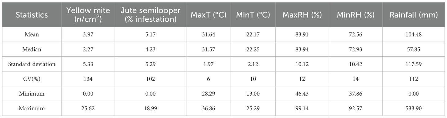
Table 1. Descriptive statistics of pest incidence and weather variables in the current week.

Seasonal incidence

The seasonal plots of yellow mite and jute semilooper are presented in Figures 1 and 2, respectively. For both pests, peak incidence is observed on 55 DAS followed by 45 DAS. The results of the WO test in Table 2 indicate that seasonality is present for jute semilooper but is absent for yellow mite.

Figure 1

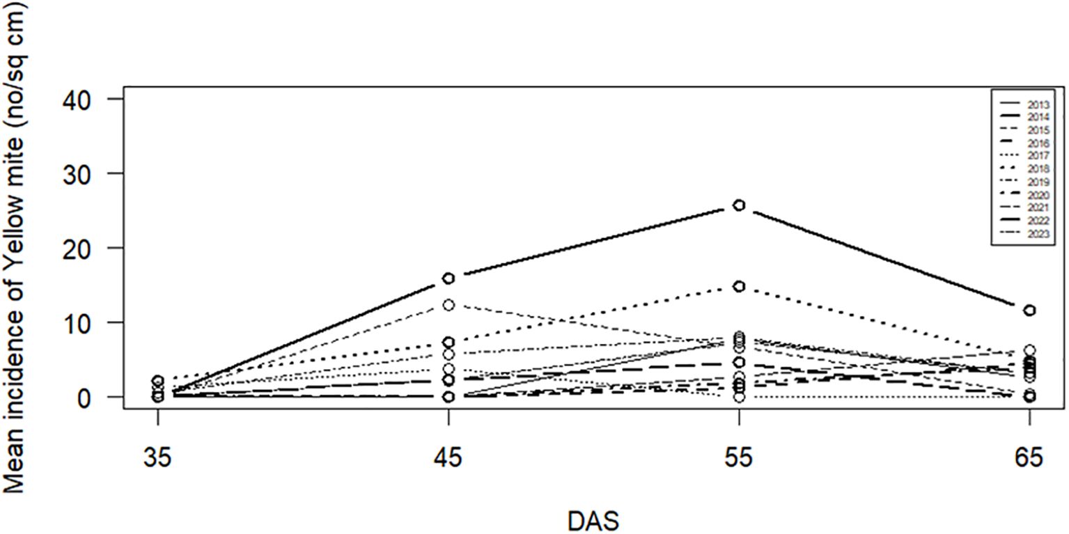
Figure 1. Seasonal plot of yellow mite incidence.

Figure 2

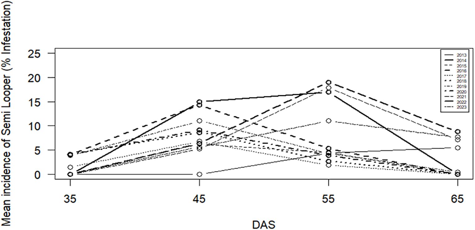
Figure 2. Seasonal plot of jute semilooper incidence.

Table 2

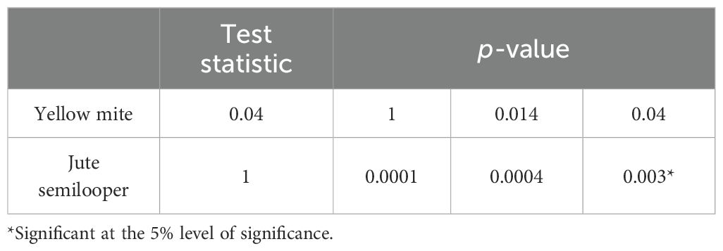
Table 2. WO test to check seasonality.

Correlation analysis

Results of Pearson’s correlation analysis in Table 3 reveal that the mean incidence of yellow mite is significantly positively correlated with maximum temperature at a 2-week lag, whereas it is significantly negatively correlated with maximum RH at a 1-week lag, and minimum and maximum RH at a 2-week lag. Similarly, the mean incidence of jute semilooper is also significantly positively correlated with maximum temperature at a 2-week lag, whereas it is significantly negatively correlated with maximum and minimum RH at a 2-week lag. The weather variables that are significantly correlated with pest incidence are further subjected to multicollinearity analysis. The results of multicollinearity analysis in Table 4 reveal that maximum and minimum RH at a 2-week lag show moderate multicollinearity for yellow mite incidence, whereas for jute semilooper, minimum RH at a 2-week lag shows moderate multicollinearity. Therefore, maximum RH at a 1-week lag and maximum temperature at a 2-week lag are to be used as exogenous variables in time series models for yellow mite incidence, whereas for jute semilooper, the exogenous variables are maximum temperature and maximum RH at a 2-week lag.

Table 3

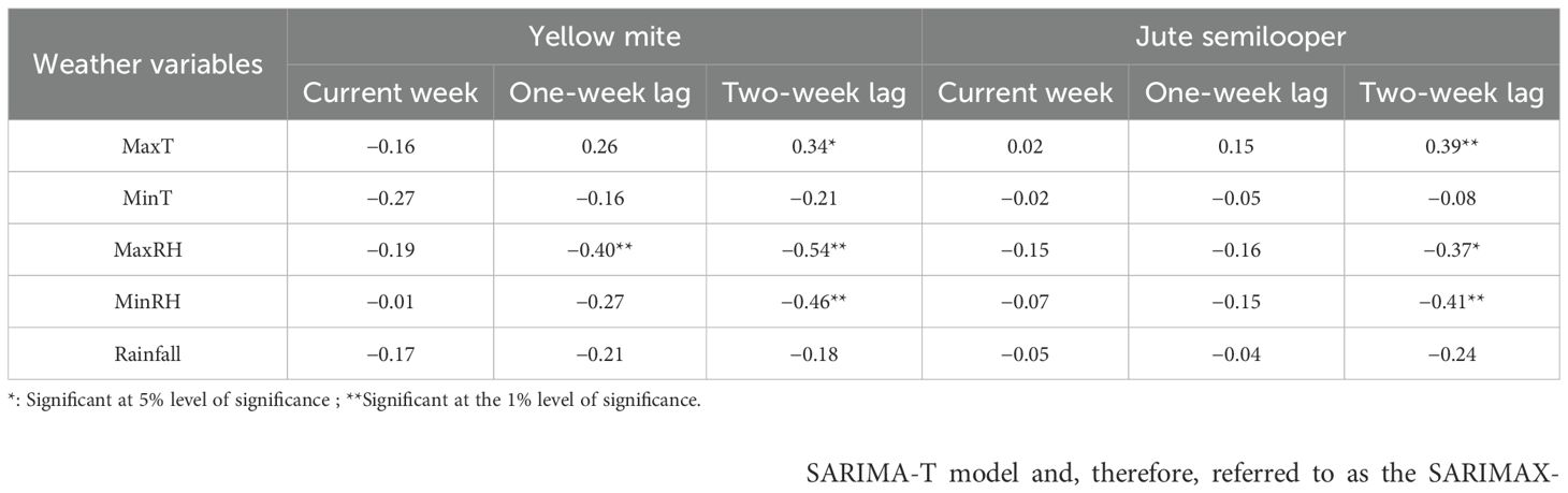
Table 3. Correlation between the mean incidence of pests with weather variables.

Table 4

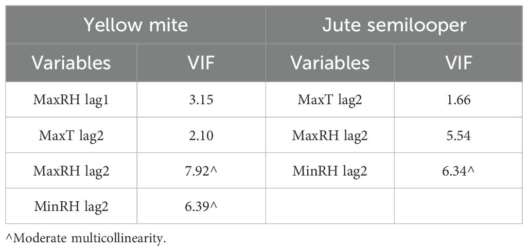
Table 4. VIF values of significantly correlated weather variables.

Fitting of different models for yellow mite and jute semilooper incidence

To check the presence of stationarity in the data series, the Augmented Dickey–Fuller (ADF) test and Phillips–Perron (PP) test have been applied, and the results are presented in Table 5. It is found that the both data series are stationary and, therefore, regular differencing is not required.

Table 5

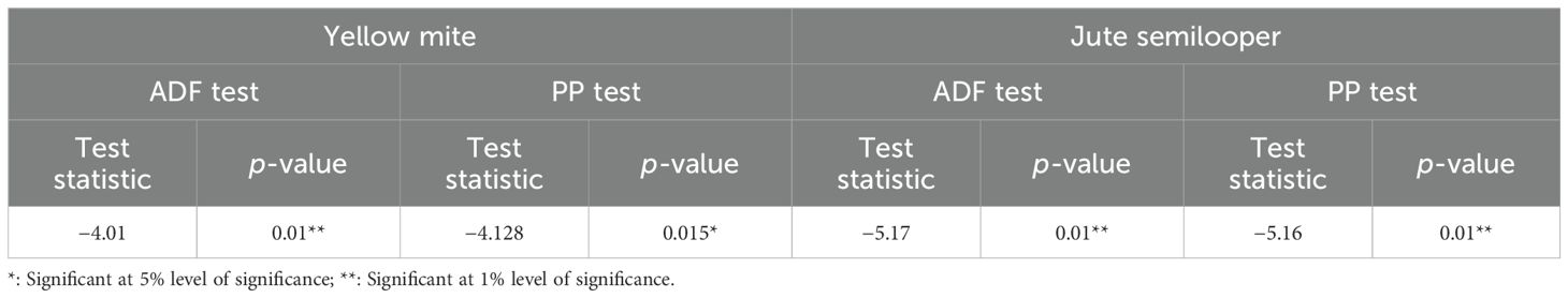
Table 5. ADF and PP test for stationarity.

After confirming the stationarity of the time series data of yellow mite incidence, an ARIMA model is fitted and the parameters are presented in Table 6. The residuals of the fitted ARIMA model are found to be non-normal, as evident from Table 7; therefore, the original data series is transformed using square root transformation with the addition of 0.5 as few zero values are there. The transformed data exhibit seasonality as evident from the WO test, and therefore, a suitable SARIMA model is fitted based on the minimum AIC and BIC criteria, and this model is referred to as SARIMA-T. The parameters of the fitted SARIMA-T model are also presented in Table 6. Subsequently, MaxRH at 1 week and MaxT at 2 weeks are used as exogenous variables in the SARIMA-T model and, therefore, referred to as the SARIMAX-T model.

Table 6

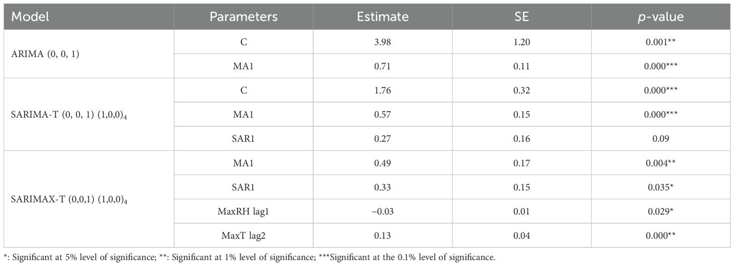
Table 6. Parameter estimates of the ARIMA (0, 0, 1), SARIMA-T (0, 0, 1) (1,0,0)₄, and SARIMAX-T (0,0,1) (1,0,0)₄ models for yellow mite incidence.

Table 7

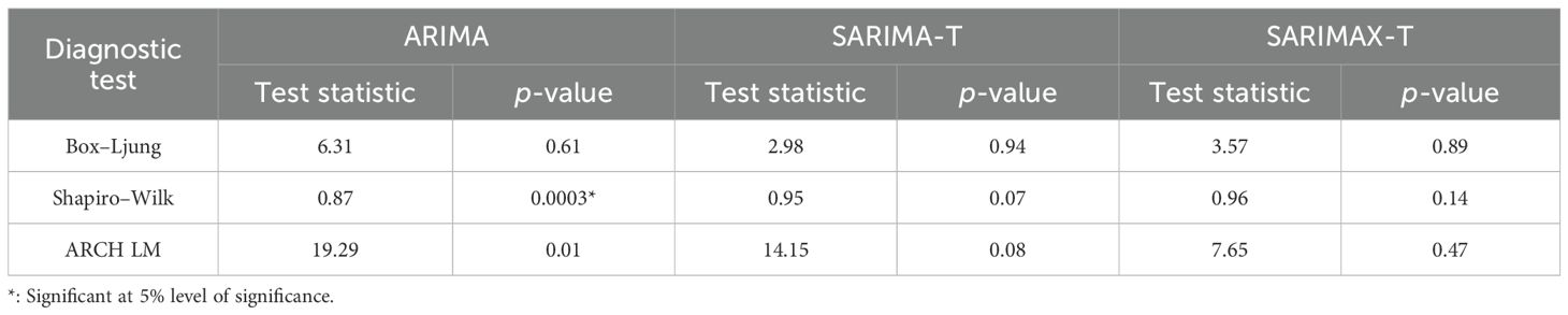
Table 7. Residual diagnostics test for time series models of yellow mite incidence.

Similarly, the results of ADF and PP tests for jute semilooper incidence in Table 4 indicate that the data series is stationary, and the WO test in Table 2 indicates that the series is seasonal. Therefore, the SARIMA model is fitted to predict the incidence of jute semilooper and the parameters of the model are presented in Table 8. Since the residuals of the fitted SARIMA model depict non-normality as evident from Table 9, square root transformation is therefore applied on the original data with the addition of 0.5 to it. The WO test on the square root transformed data of semilooper incidence indicates non-seasonality, and accordingly, the ARIMA (2, 0, 1) model is fitted on this transformed data, and subsequently, the model is referred to as ARIMA-T. The parameters of the fitted ARIMA-T model are also presented in Table 8. In case of jute semilooper, MaxT and MaxRH at 2 weeks are found to be the most important exogenous variables. Therefore, ARIMAX (3,1,0) is found to be the best fitted model on the original time series data of jute semilooper incidence. The parameter estimates with standard error (SE) and p-values are presented in Table 8. However, the residuals of fitted ARIMAX model are found to be non-normal and therefore, ARIMAX model is fitted on the square root transformed data. This model is referred to as ARIMAX-T. The estimate of parameters, its SE, and the respective p-values are also presented in Table 8.

Table 8

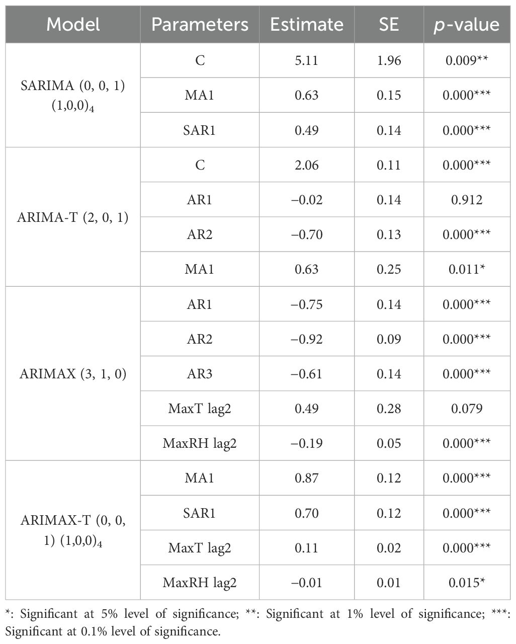
Table 8. Parameter estimates of the SARIMA (0, 0, 1) (1,0,0)₄, ARIMA-T (2, 0, 1), ARIMAX (3, 1, 0), and SARIMAX-T (0, 0, 1) (1,0,0)₄ models for jute semilooper incidence.

Table 9

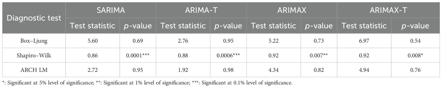
Table 9. Residual diagnostics test for time series models of jute semilooper incidence.

Random Forest relies on two key algorithms: bagging and random feature selection. Bagging involves selecting a specified number of samples (ntree) from the dataset using simple random sampling with replacement (SRSWR) to construct multiple trees. Random feature selection determines the number of variables (mtry) to consider at each split. The hyperparameters of the fitted Random Forest model are provided in Table 10. The Random Forest model also evaluates the % increase in node impurity (IncNodePurity) to identify important variables. For predicting the mean incidence of yellow mite, rainfall and MaxT at a 2-week lag are identified as significant weather variables, as shown in Figure 3. Similarly, for predicting the jute semilooper incidence, rainfall and MaxT at a 2-week lag are also recognized as important weather variables, as shown in Figure 4. The key weather variables identified from the variance importance plot in the Random Forest model, rainfall and MaxT at a 2-week lag, are used as exogenous variables in both the SVR and TDNNX models.

Table 10

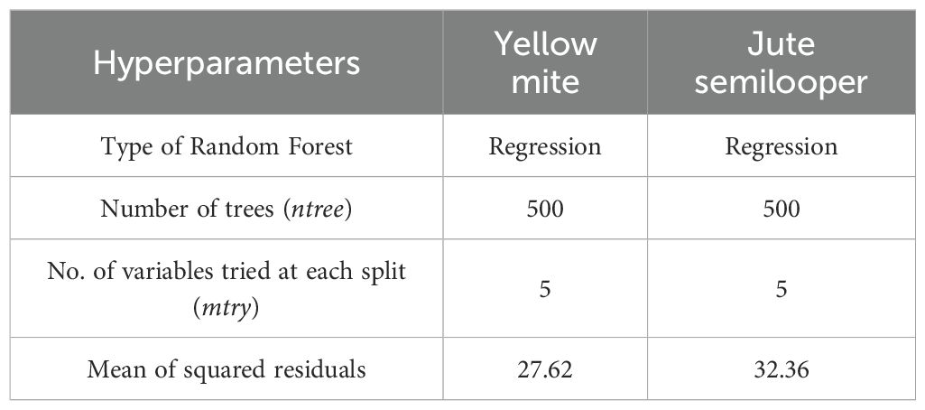
Table 10. Hyperparameters of the Random Forest model for both yellow mite and jute semilooper incidences.

Figure 3

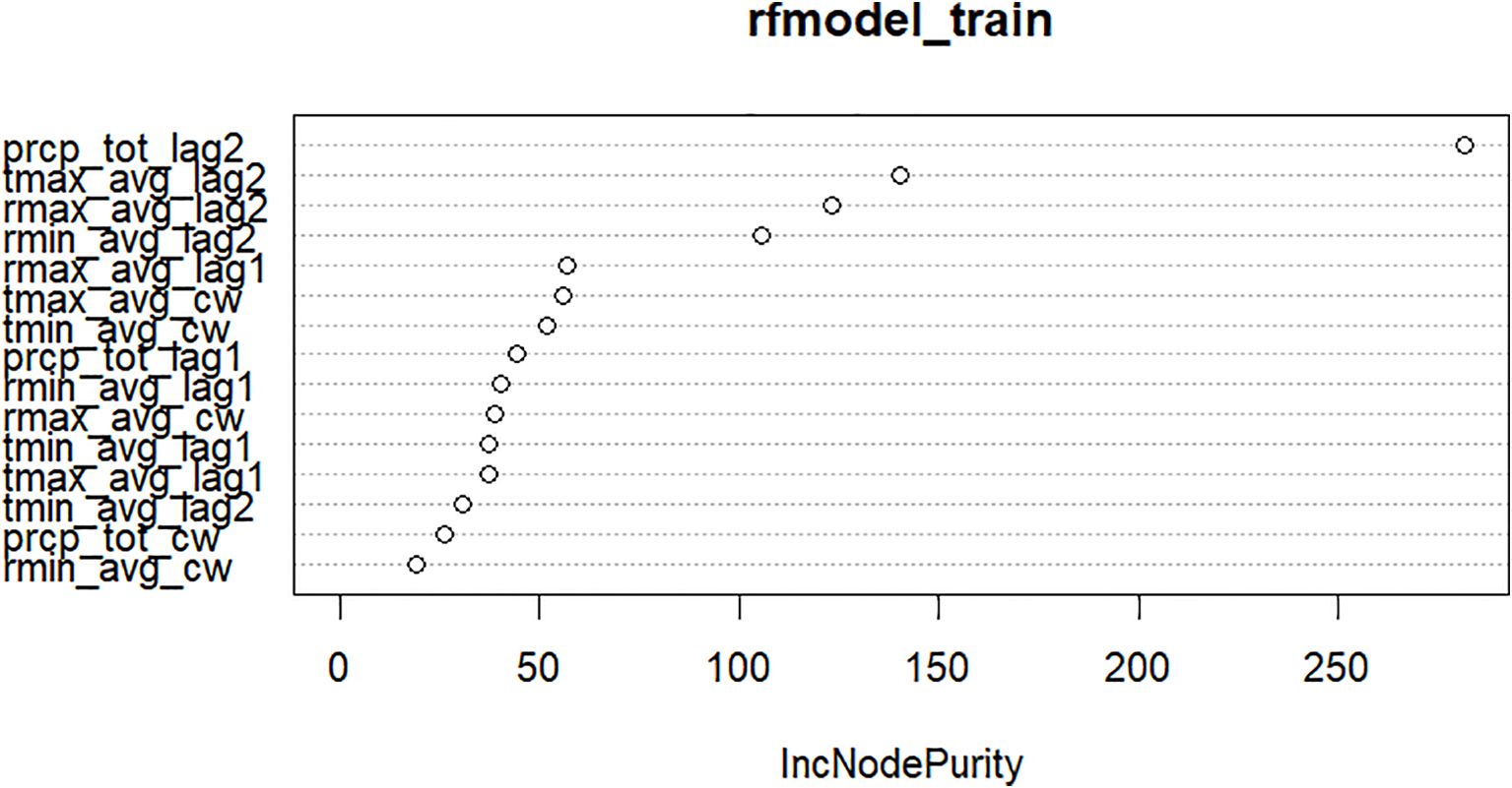
Figure 3. Variable importance plot of the Random Forest model for yellow mite incidence.

Figure 4

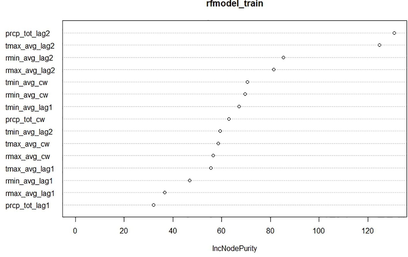
Figure 4. Variable importance plot of the Random Forest model for jute semilooper incidence.

For both pests, the SVR model is trained with the mean incidence as the dependent variable and rainfall and MaxT at a 2-week lag as the exogenous variables. The hyperparameters of the fitted SVR model are provided in Table 11.

Table 11

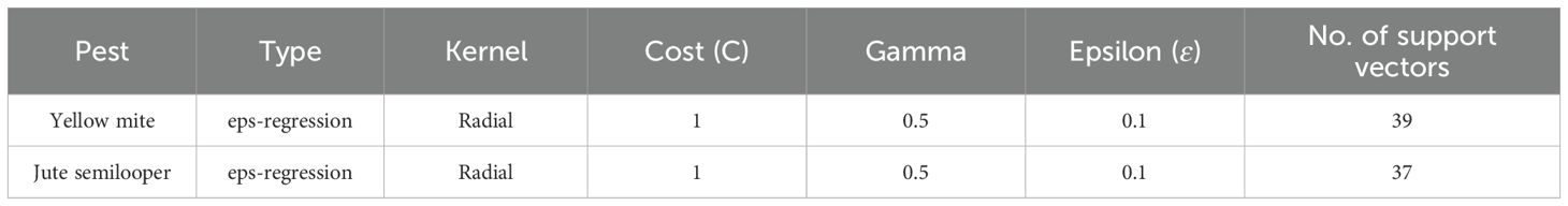
Table 11. Hyperparameters of the SVR model for both yellow mite and jute semilooper incidences.

The TDNNX model is fitted between the mean incidence of pest with its lagged values up to the significant order and exogenous weather variables selected from the Random Forest model. In the TDNNX (p,k) model, p and k indicate the number of nodes in the input and hidden layer, respectively. For both yellow mite and semilooper incidences, there are five nodes in the input layer that correspond to lagged values of mean pest incidence up to the order of three and two exogenous weather variables. The hyperparameters of the fitted TDNNX model are presented in Table 12.

Table 12

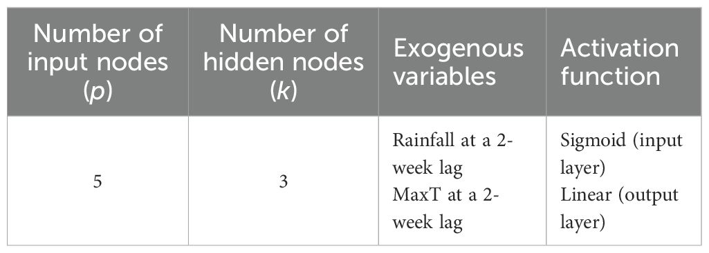
Table 12. Hyperparameters of the TDNNX model for both yellow mite and jute semilooper incidences.

Model validation

The predictive abilities of different time series and machine learning models are compared using RMSE and RMdSE as the evaluation criteria for both training and testing dataset, and the results are presented in Table 13. For the mean incidence of yellow mite, TDNNX is found to be the best fitted model followed by SVR and SARIMA-T on the basis of RMSE and RMdSE values. Similarly, for jute semilooper, it is observed that the TDNNX model produces the least RMSE and RMdSE value for the training dataset followed by Random Forest, but for the testing dataset, SARIMA has the least RMSE values followed by Random Forest and TDNNX. However, the residuals of the fitted SARIMA model are not normally distributed, and therefore, model assumptions are violated. Thus, by considering both RMSE and RMdSE values, TDNNX may also be considered as the best fitted model for prediction of the mean incidence of jute semilooper followed by Random Forest and SARIMA. The plots of observed vs. fitted values for the mean incidence of yellow mite and jute semilooper across different models are shown in Figures 5 and 6, respectively.

Table 13

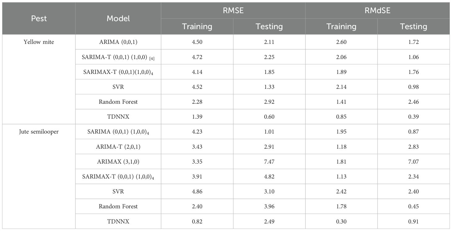
Table 13. Predictive abilities of different models for both yellow mite and jute semilooper incidences.

Figure 5

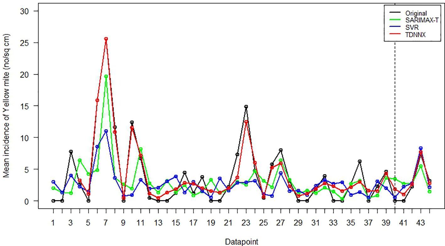
Figure 5. Plot of observed vs. fitted values by SARIMAX-T, SVR, and TDNNX models for yellow mite incidence.

Figure 6

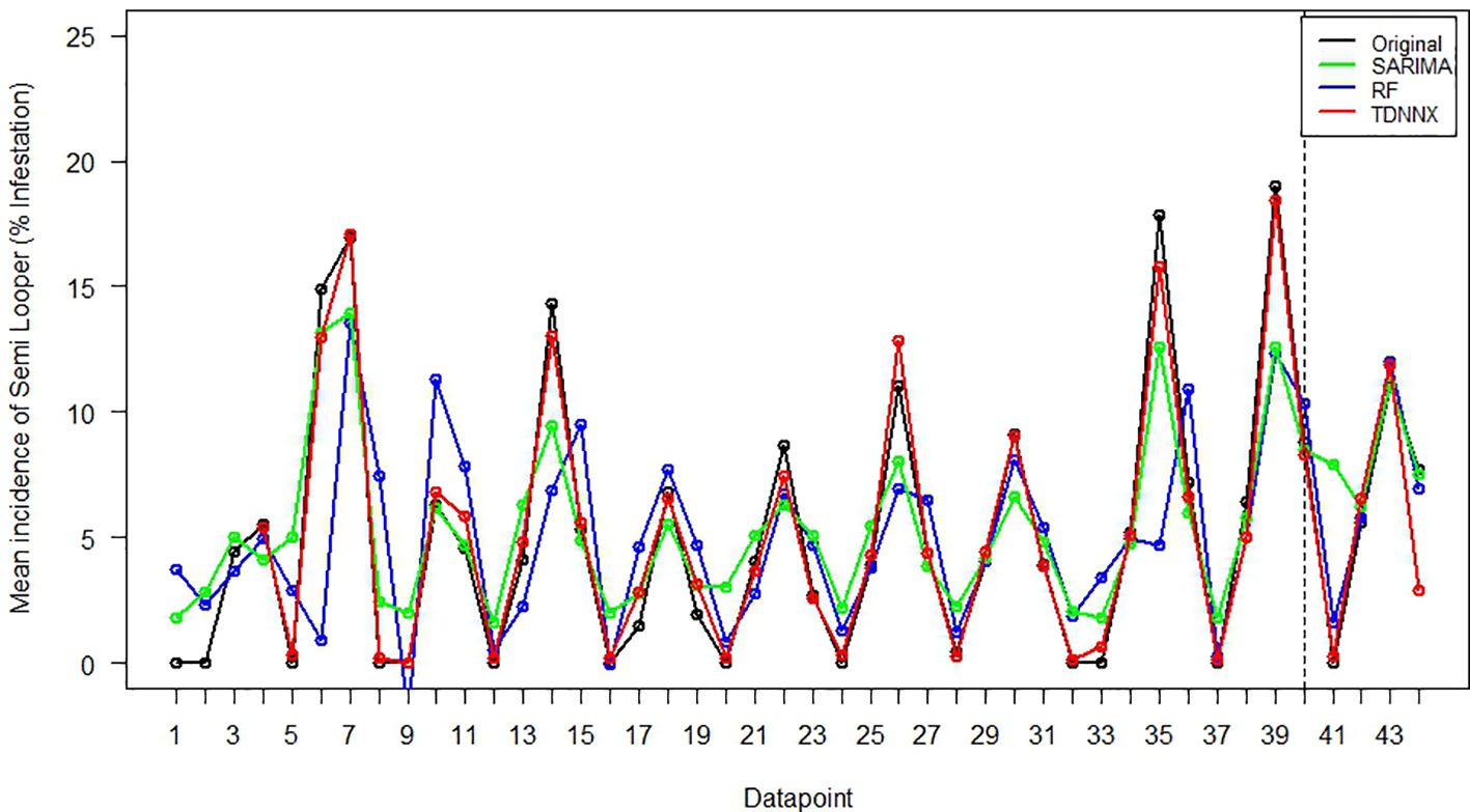
Figure 6. Plot of observed vs. fitted values of SARIMA, Random Forest, and TDNNX models for semilooper incidence.

Forecasting of pest incidence

The out-of-sample forecasts for pest incidence of yellow mite and jute semilooper are obtained using the TDNNX model for the year 2024 at 35, 45, 55, and 65 DAS. The forecasts are obtained using forecasted values of weather variables, i.e., rainfall and MaxT at a 2-week lag, from the ARIMA model, and the results are presented in Table 14. Additionally, out-of-sample forecasts of pest incidence are also made using the average values of weather variables (rainfall and MaxT at a 2-week lag) for the period from 2013 to 2023, and the results are presented in Table 15.

Table 14

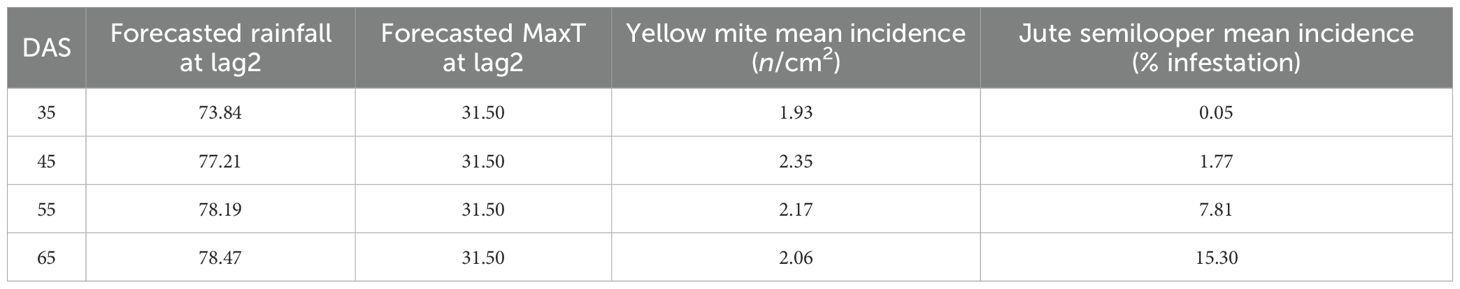
Table 14. Out-of-sample forecast for the mean incidence of yellow mite and jute semilooper for the year 2024 using forecasted weather data.

Table 15

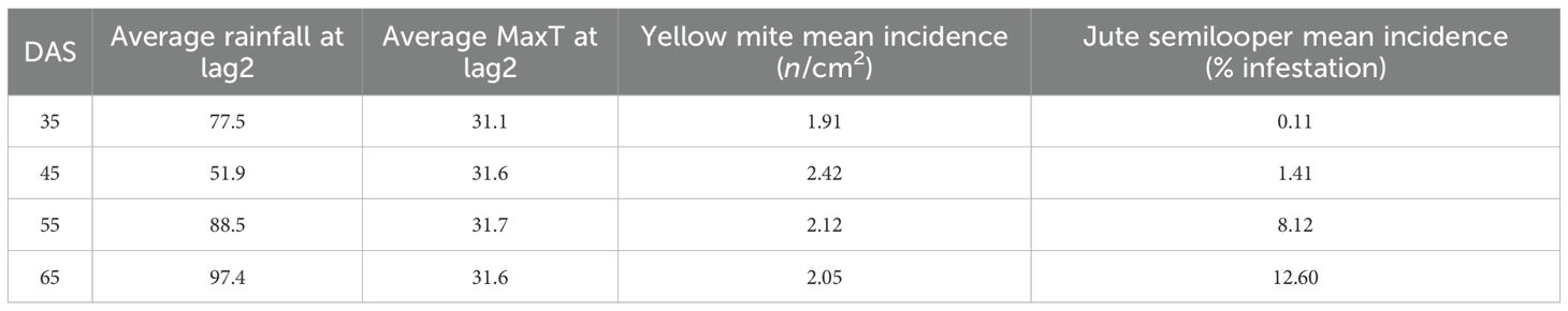
Table 15. Out-of-sample forecast for the mean incidence of yellow mite and jute semilooper for the year 2024 using average weather data from 2013 to 2023.

Conclusion

The study found that the peak mean incidence of jute semilooper and yellow mite occurs at 45 and 55 DAS, respectively, with seasonality observed only in jute semilooper. Among the crop years studied, the peak mean incidence of yellow mite was recorded in 2014, while for jute semilooper, it occurred in 2022. The study also revealed that incidence of yellow mite has a significant positive correlation with maximum temperature at a 2-week lag while the correlation with maximum relative humidity at a 1- and 2-week lag is highly significant in a negative direction. This suggests that dry weather with high temperatures 2 weeks prior leads to higher yellow mite infestations at present. Consequently, if such weather conditions are observed, there is a likelihood of increased mite infestation in the following 2 weeks. This information can assist farmers in better preparing for pest emergence and in making informed decisions regarding pest control measures. Among the different time series and machine learning models, the TDNNX model was found to be the most accurate for predicting the mean incidence of both yellow mite and jute semilooper using weather variables.

Data availability statement

The raw data supporting the conclusions of this article will be made available by the authors, without undue reservation.

Author contributions

PB: Writing – review & editing, Conceptualization, Writing – original draft. SS: Investigation, Writing – original draft, Writing – review & editing. DG: Supervision, Writing – review & editing, Writing – original draft. TP: Visualization, Methodology, Writing – review & editing. MD: Software, Writing – review & editing. PS: Writing – review & editing, Visualization. SH: Writing – review & editing, Data curation. SK: Supervision, Writing – review & editing.

Funding

The author(s) declare that no financial support was received for the research and/or publication of this article.

Conflict of interest

The authors declare that the research was conducted in the absence of any commercial or financial relationships that could be construed as a potential conflict of interest.

Generative AI statement

The author(s) declare that no Generative AI was used in the creation of this manuscript.

Any alternative text (alt text) provided alongside figures in this article has been generated by Frontiers with the support of artificial intelligence and reasonable efforts have been made to ensure accuracy, including review by the authors wherever possible. If you identify any issues, please contact us.

Publisher’s note

All claims expressed in this article are solely those of the authors and do not necessarily represent those of their affiliated organizations, or those of the publisher, the editors and the reviewers. Any product that may be evaluated in this article, or claim that may be made by its manufacturer, is not guaranteed or endorsed by the publisher.

References

Balikai R. A. and Venkatesh H. (2019). Weather based prediction models to forecast major pests of rabi sorghum in Karnataka, India. J. Exp. Zool. India 22, 131–134.

Google Scholar

Bierens H. J. (1987). ARMAX model specification testing, with an application to unemployment in the Netherlands. J. Econom. 35, 161–190. doi: 10.1016/0304-4076(87)90086-8

Crossref Full Text | Google Scholar

Box G. E. P. and Jenkins G. M. (1976). Time Series Analysis: Forecasting and Control. Revised Edition (San Francisco: Holden Day).

Google Scholar

Breiman L. (2001). Random forests. Mach. Learn 45, 5–32. doi: 10.1023/A:1010933404324

Crossref Full Text | Google Scholar

Chai T. and Draxler R. R. (2014). Root mean square error (RMSE) or mean absolute error (MAE)? – Arguments against avoiding RMSE in the literature. Geosci. Model. Dev. 7, 1247–1250. doi: 10.5194/gmd-7-1247-2014

Crossref Full Text | Google Scholar

Durgabai R. P. L. and Bhargavi P. (2018). Pest management using machine learning algorithms: a review. Int. J. Comp. Sci. Eng. Info. Tech. Res. 8, 13–22.

Google Scholar

Hussain M., Rahman M., Uddin M. N., Taher M. A., Nabi M. N., and Mollah A. F. (2002). Problems and solutions in jute cultivation faced by the farmers in a selected area of Bangladesh. J. Biol. Sci. 2 (9), 628–629. doi: 10.3923/jbs.2002.628.629

Crossref Full Text | Google Scholar

Hyndman R. J. and Athanasopoulos G. (2021). Forecasting: Principles and Practice (3rd ed.) (Melbourne, Australia: OTexts).

Google Scholar

Hyndman R. J. and Koehler A. B. (2006). Another look at measures of forecast accuracy. Int. J. Forecast 22, 679–688. doi: 10.1016/j.ijforecast.2006.03.001

Crossref Full Text | Google Scholar

Katke M. K., Balikai R. A., and Venkatesh H. (2009). Seasonal incidence of grape mealy bug, Maconellicoccus hirsutus (green) and its relation with weather parameters. Pest Mgmt. Hortic. Eco. 15, 9–16.

Google Scholar

Rahman S. and Khan M. R. (2012). Incidence of pests in jute (Corchorus olitorius L.) ecosystem and pest–weather relationships in West Bengal, India. Arch. Phyto. Pl Protec 45, 591–607. doi: 10.1080/03235408.2011.588053

Crossref Full Text | Google Scholar

Sarkar P., Basak P., Panda C. S., Gupta D. S., and Ray M. (2023). Prediction of peak pest population incidences in jute crop based on weather variables using statistical and machine learning models: A case study from West Bengal. J. Agrometeorol. 25, 305–311. doi: 10.54386/jam.v25i2.1915

Crossref Full Text | Google Scholar

Sarkar S. and Majumdar B. (2016). Present status of jute production and technological and social interventions needed for making jute agriculture sustainable and remunerative in West Bengal. Indian J. Nat. Fib. 3, 23–36.

Google Scholar

Suyal P., Gaur N., Rukesh P. K. N., and Devrani A. (2018). Seasonal incidence of insect pests and their natural enemies on soybean crop. J. Entomon. Zoo Stud. 6, 1237–1240.

Google Scholar

Vaidheki M., Gupta D. S., Basak P., Debnath M. K., Hembram S., and Ajith S. (2023). Prediction of potato late blight disease severity based on weather variables using statistical and machine learning models: A case study from West Bengal. J. Agrometeorol. 25, 583–588. doi: 10.54386/jam.v25i4.2272

Crossref Full Text | Google Scholar

Vapnik V. N. (2000). The Nature of Statistical Learning Theory. 2nd Edition (Berlin: Springer). doi: 10.1007/978-1-4757-3264-1

Crossref Full Text | Google Scholar