Integrated modelling of shading effects on alfalfa growth across different agrivoltaic systems

Introduction: Agrivoltaic systems (AVS) combine agricultural production with solar energy generation on the same land. However, the spatiotemporal variability in light availability caused by panel shading presents a critical challenge for accurately predicting impacts on crop growth and yield.

Methods: This study introduces a novel modeling framework that integrates a three-dimensional radiative model with a process-based crop growth model, implemented in the GroIMP platform, to simulate the performance of alfalfa (Medicago sativa L.) under contrasting AVS conditions. The model accounts for dynamic light interception, canopy temperature variation, and soil water availability. Field experiments were conducted in northern and central Italy under three conditions: open field (Site A), fixed-panel AVS (Site B), and bi-axial tracking AVS (Site C).

Results and discussion: The model was, the model was calibrated and validated using field data on leaf area index (LAI) (R² ≥ 0.79, RMSE ≤ 48.61), dry matter yield (R² ≥ 0.82, RMSE ≤ 48.6 g m⁻²) and canopy temperature (R² = 0.83, RMSE = 1.24 °C), demonstrating strong agreement with observations. The validated model enabled a detailed assessment of how different panel configurations influence microclimatic conditions, which in turn significantly affected alfalfa growth and biomass production. From this perspective, simulations revealed pronounced spatial gradients driven by shading intensity, system layout, and seasonal dynamics, emphasizing the critical role of AVS design in determining crop performance. In particular, yield differences among treatments reflected microclimatic modifications induced by the panels, with shading and rainfall redistribution likely affecting canopy temperature, soil moisture dynamics, and associated plant water relations.

Conclusions: The proposed integrated modeling framework thus provides a robust and scalable tool for AVS design and management, supporting both agronomic planning and the optimization of structural configurations tailored to site-specific climatic conditions. By doing so, it may effectively contribute to the development of more adaptive, efficient, and sustainable agri-energy systems capable of balancing agricultural productivity with renewable energy generation.

GRAPHICAL ABSTRACT

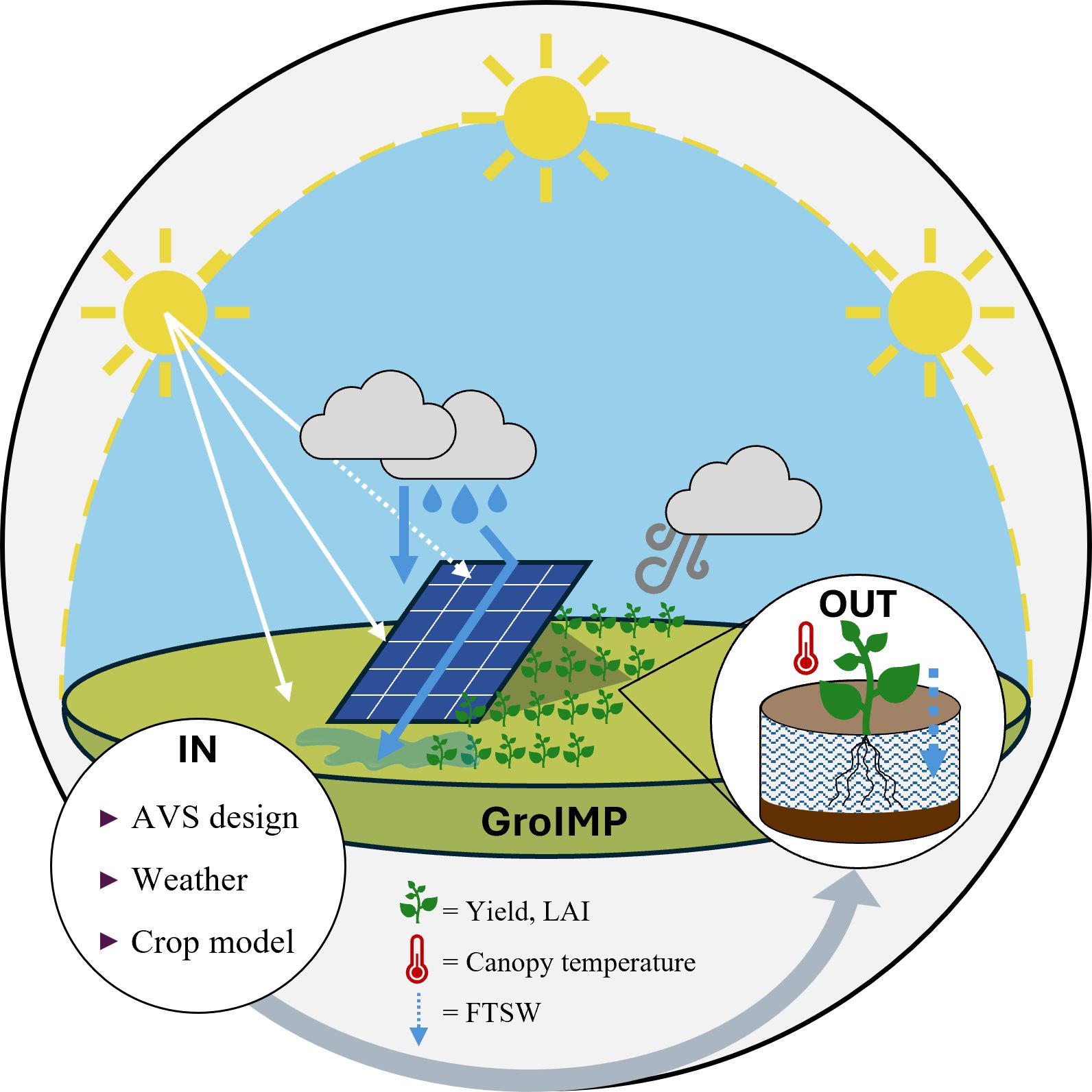
Graphical Abstract.

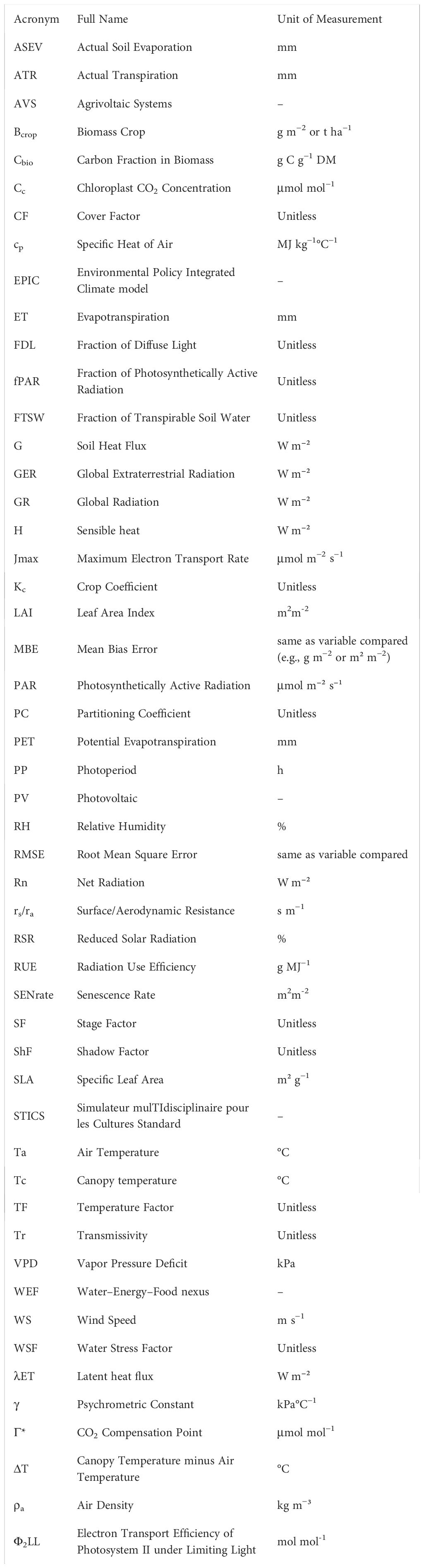
Nomenclature

.

1 Introduction

Agrivoltaic systems (AVS) are increasingly recognized as a promising solution to address the interlinked challenges of the Water–Energy–Food (WEF) nexus by integrating agricultural production with renewable energy generation on the same land area (Barron-Gafford et al., 2019). However, this dual-use approach inherently entails trade-offs between crop performance and solar energy capture, making it essential to optimize system design for both efficiency and long-term sustainability. At the same time, the electricity generated by AVS can directly power on-farm operations such as irrigation, cooling, or processing, or be exported to the grid, thereby reducing greenhouse gas emissions and creating an additional source of income that reinforces the overall sustainability of the system (Agostini et al., 2021). A key aspect of this optimization lies in understanding how the partial or complete shading induced by photovoltaic (PV) panels alters microenvironmental conditions, particularly light availability, temperature regimes, and soil moisture dynamics, which in turn can significantly affect crop growth and development (Marrou et al., 2013; Ma et al., 2022).

Assessing the complex interactions between AVS components and the physiological drivers of plant response under variable shading is therefore critical to evaluating overall system performance (Choi et al., 2023). Reduced solar radiation has been identified as the primary constraint to crop productivity in AVS (Marrou et al., 2013), leading countries to establish regulatory limits on Ground Coverage Ratios (e.g., Italy, with a 40% GCR limit; Dupraz, 2024). Consequently, ongoing research is increasingly focused on quantifying the heterogeneous impacts of AVS, which depend on the interaction between species-specific sensitivity to shading and the growing season. As outlined by the meta-analysis in Laub et al. (2022), the response of different cultivated species to increasing shading is non-linear. While most crops analyzed (berries, fruits, fruiting vegetables, and forages) tolerate moderate shading, maize and grain legumes exhibit a strong yield reduction even under low shading conditions. In any case, for shading greater than 50%, all the crops proved to be susceptible. However, seasonal variability and management practices also strongly interact with a crop’s response to shading. As an example, a two-year field trial on alfalfa recorded a season-by-season effect of moderate shading (25-30%) from PV panels on biomass production where shading proved particularly beneficial during drought periods resulting in increased biomass accumulation (+10%) with respect to full sunlight (Edouard et al., 2023). Wheat, considered a species sensitive to decreased radiation, exhibits different responses not only between varieties but also in response to the prevailing climatic conditions. Laub et al. (2022) observed that in subtropical environments, wheat-maintained yields comparable to open field conditions under low shading, 30% reduced solar radiation (RSR level), while higher levels of shading resulted in an average yield reduction of 36.2%. Conversely, in temperate regions experiencing low shading levels, a decline in yield of 17.4% and 45.2% was observed under shading conditions exceeding 30% RSR level. These findings emphasize the climate-dependent plasticity of crop responses to shading.

Although existing studies highlight both the opportunities and challenges of AVS deployment, they also expose a major knowledge gap: current evidence remains largely crop- and context-specific, which limits the transferability of results across environmental and agronomic conditions (Laub et al., 2022; Marrou et al., 2013; Amaducci et al., 2018). The strong species-specific responses to shading, combined with the spatio-temporal variability of microclimates induced by photovoltaic structures, underscore the need for systematic data collection across diverse climates and AVS configurations. Yet, the labor and time-intensive nature of field campaigns constrain large-scale evaluations, positioning modelling frameworks as a powerful alternative for assessing AVS impacts on crop performance and resource-use efficiency (Zainali et al., 2025).

Two- (2D) and three-dimensional (3D) simulation platforms coupled with crop growth models, such as EPIC (Campana et al., 2024), GECROS (Amaducci et al., 2018; Bellone et al., 2024), and STICS (Dupraz et al., 2011; Dinesh and Pearce, 2016; Crépeau et al., 2025), have become increasingly common for simulating radiation dynamics, light interception, and biomass production under heterogeneous conditions, including AVS (Grubbs et al., 2024). These tools have significantly accelerated the evaluation of crop-specific shading responses and the identification of optimal AVS designs balancing energy and agricultural outputs (Bellone et al., 2024). Despite advances in modeling crop-radiation interactions, key methodological gaps remain. Daily-step models (e.g., STICS, EPIC) cannot resolve intra-day radiation dynamics, and even hourly models like GECROS lack full 3D integration to represent canopy light distribution. Moreover, most approaches treat photovoltaic and crop growth modules separately, limiting the understanding of soil-water redistribution and its impact on productivity and system efficiency. Nonetheless, a major limitation persists due to the lack of robust, multi-seasonal experimental datasets for model calibration and validation (Zainali et al., 2025). Where data are available, they are often restricted to a single growing season, limiting the ability to capture interannual variability. This constraint is highlighted by recent studies emphasizing the scarcity of long-term data in European contexts, which undermines the reliability and transferability of the existing models (Zidane et al., 2025; Berrian et al., 2025). For such an example, Mazzeo et al. (2025) proposed a sophisticated simulation approach, yet acknowledged that many yield estimates are still derived from artificially shaded experiments rather than real AVS conditions.

Another critical source of uncertainty concerns the type of crop growth model used to estimate biomass responses under AVS conditions. Broadly, these models can be classified into two categories. The first refers to semi-mechanistic models, which simulate crop development on a daily time step using simplified assumptions, most notably, Radiation Use Efficiency to convert intercepted light into biomass (Monteith, 1977; Brisson et al., 2002). The second includes process-based models, which rely on a detailed, physiological representation of photosynthesis, operating typically on an hourly scale and incorporating key limiting factors such as water and nitrogen availability (Kirschbaum et al., 1997; Morales et al., 2018; Bellasio, 2019). Semi-mechanistic models are generally easier to parameterize and calibrate due to their lower data requirements, making them suitable for broad-scale applications. However, they may lack the resolution needed to capture intra-daily shading fluctuations typical of AVS, thus limiting their accuracy in highly dynamic light environments (He et al., 2024; Zainali et al., 2025). In contrast, process-based models are better equipped to simulate the fine-scale effects of fluctuating radiation, but they require extensive input data, including crop-specific biochemical and structural parameters, which are often unavailable or difficult to measure (Prusinkiewicz and Runions, 2012).

Building upon these premises, this study presents the development and validation of a novel modelling framework that integrates a simplified process-based crop growth model with a high-resolution, three-dimensional radiative environment. The framework is specifically designed to resolve the spatial and temporal heterogeneity of intra-daily shading patterns generated by diverse AVS configurations, while capturing feedback processes that are fundamental for a realistic representation of crop productivity under fluctuating light regimes. Its performance was rigorously evaluated using an extensive multi-year dataset collected across contrasting environmental contexts, including open-field conditions, fixed-panel installations, and dual-axis tracking AVS, with alfalfa (Medicago sativa L.) employed as a representative model species.

2 Materials and methods

2.1 Study area and experimental design

Field trials were conducted across three locations in northern and central Italy (Figure 1), each representing a distinct agronomic and environmental context: (i) an open-field reference site in Montese (Modena; Figure 1-Site A), (ii) a fixed-panel AVS in Sant’alberto (Ravenna; Figure 1-Site B), and (iii) a bi-axial tracking AVS in Borgo Virgilio (Mantova; Figure 1-Site C). These sites were selected to capture a range of radiation regimes and to assess crop performance under different spatial and temporal shading conditions.

Figure 1

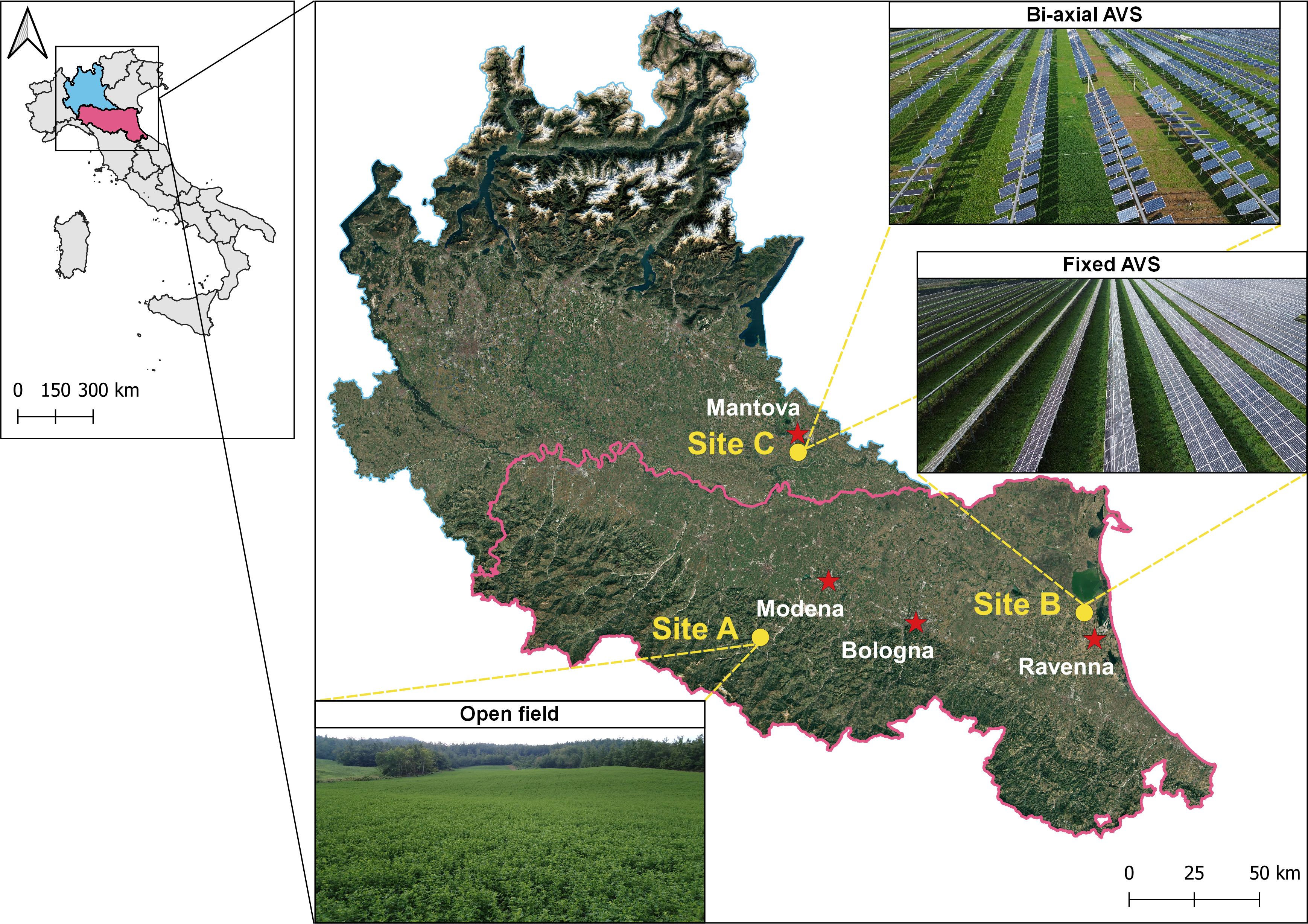
Figure 1. Location of the open field (Site A), fixed (Site B) and bi-axial (Site C) agrivoltaic system experimental sites.

2.1.1 Open-field setup

The open-field study area is located within the ‘Terre di Montagna’ Consortium, which includes approximately 100 farms dedicated to Parmigiano Reggiano production in the mountainous Apennine regions of Bologna and Modena (Emilia-Romagna, central Italy), at altitudes exceeding 600 meters above sea level. The local soils are mainly composed of sandstone, limestone, and marl, exhibiting variable pH conditions. Climatic data were obtained from the Montese meteorological station (44.4579° N, 10.5899° E), positioned at the center of the study area (Supplementary Figure S1). The climate is characterized by an average annual temperature of 10.1°C and mean annual precipitation of 930 mm, with limited drought occurrence during the summer months (Argenti et al., 2021).

2.1.2 Fixed agrivoltaic system

The fixed AVS study site is located in Sant’Alberto (Ravenna, Italy; 44.51019° N, 12.1552° E), a northeastern area of Italy well-suited for AVS implementation due to its high solar radiation and fertile agricultural soils. The site has been operational since 2012 and hosts a 70-hectare alfalfa (Medicago sativa L.) meadow, contributing to approximately 45 GWh of electricity per year. The terrain is predominantly flat, with elevations ranging from 4 to 8 m above sea level. The climate is temperate, with hot summers and cold winters, and an average annual temperature of 15°C (ranging from 5°C in January to 25.6°C in July). Annual precipitation averages 767 mm, with November being the wettest month (87 mm) and January the driest (49 mm). Meteorological data were recorded at the local weather station throughout the experimental period (Figure 1). Soils at the site are classified as silty sand in the 0-60 cm layer, composed of 50% sand, 40% silt, and 10% clay. Photovoltaic panels at the site are mounted on south-facing ground structures tilted at a 35° angle. The tables are 3.5 m wide with 8 m spacing between rows, resulting in a Ground Cover Ratio (GCR) of 38%. Panel height varies from 1.3 m at the lower edge to 3.3 m at the upper edge (Figure 2a). Prior to sowing in 2020, the soil was plowed to a depth of 30 cm, then tilled and rolled to ensure good seed-to-soil contact, facilitating successful crop establishment under the AVS configuration.

Figure 2

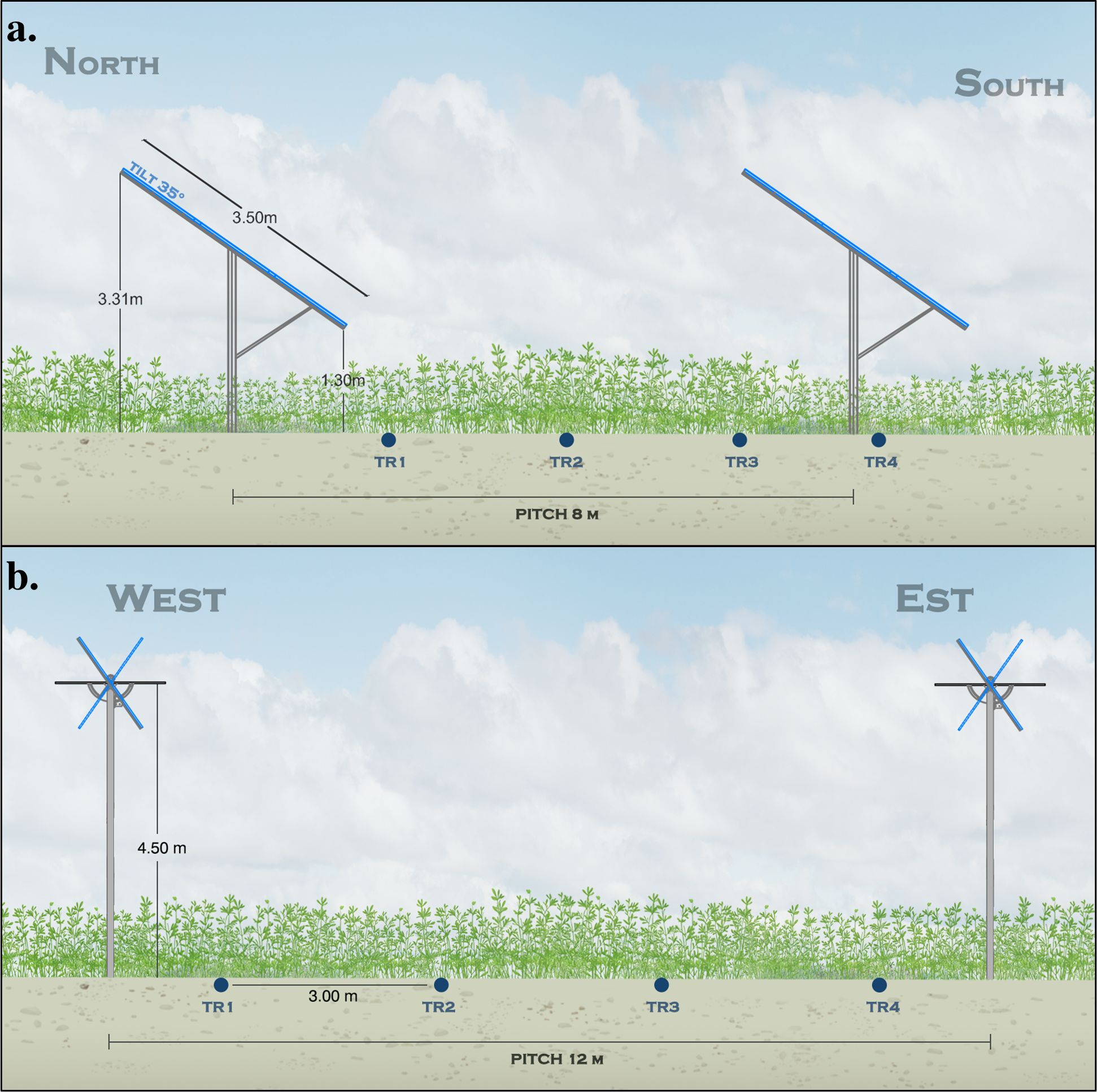
Figure 2. Representation of the fixed (a, Site B) and bi-axial AVS (b, Site C), highlighting the spacing between rows, height of the panel in relation to the ground and arrangement of treatments (TR1-TR4).

2.1.3 Bi-axial agrivoltaic system

The bi-axial AVS experimental site is located in Borgo Virgilio, northern Italy (Mantova; 45.0944° N, 10.7916° E), and has been operational since April 2011. The site spans 11.42 hectares, with approximately 13% of the surface occupied by photovoltaic panels (GCR), each measuring 1 m × 2 m. The total installed capacity is 2,150.4 kWp, distributed across 768 biaxial solar trackers that support 7,680 polycrystalline PV modules (Poly 280 Wp, Bisol Group, Slovenia). The panels are mounted 4.5 m above ground and are capable of dual-axis tracking, with tilt ranges of ±50° along the primary axis and ±40° along the secondary. Soils at the site are classified as silty sand in the 0-60 cm layer, composed of 50% sand, 40% silt, and 10% clay. The pH is slightly alkaline (8.5), with an organic carbon content of 1.1% and total nitrogen of 0.18%. Available phosphorus and exchangeable potassium levels are 76.4 mg kg⁻¹ and 810 mg kg⁻¹, respectively.

2.2 Data collection

Field data were collected at the three experimental sites - Site A, B and C - throughout the entire seasonal growth cycle of alfalfa. Measurements focused on above-ground dry biomass (AGB, g) and Leaf Area Index (LAI, m² m^-2), both used for model calibration and validation.

At the open-field site (Figure 1-Site A), surveys were conducted during the 2019 season on four-year-old pure stands of alfalfa. Sampling occurred on three dates (day of year (DOY) 150, 197, and 241), corresponding to spring, summer, and late summer, respectively. For each date, three replicate plots per field were randomly selected. On each sampling date, canopy LAI was first measured using a LI-COR ceptometer (LI-190; LI-COR, USA), with one reading per plot. Subsequently, AGB was harvested within 0.5 × 0.5 m quadrats using battery-powered clippers, following the protocol of Mikhailova et al. (2000). Samples were sealed in plastic bags, transported to the laboratory, and oven-dried at 80°C for 48 hours until constant weight (Wang et al., 2019).

At the fixed AVS site (Figure 1-Site B), sampling was performed throughout the 2023 and 2024 growing seasons on the following dates: DOY 7, 68, 144, 188, 212, and 314 (2023) and DOY 80, 100, 191, and 268 (2024). A total of 36 sample plots (0.5 × 0.5 m each) were established according to a randomized complete block design, consisting of four treatments (TR1: 6% shading, TR2: 7% shading, TR3: 67% shading, TR4: 82% shading) replicated three times within each of the three blocks distributed across the field (Figure 2a). This layout allowed for the capture of both spatial heterogeneity and treatment effects across the AVS. Plots were systematically positioned along the shading gradient imposed by the PV panels. On each sampling date, canopy LAI was first measured using an AccuPAR LP-80^® ceptometer (Decagon Devices, Pullman, WA, USA). Subsequently, regrowth biomass was harvested to a height of 3 cm within the 0.5 × 0.5 m frame at the plot center. Samples were dried at 60°C for 48 hours to determine dry matter yield (g m^-2). For a detailed description of the site and the relevant sampling protocol, please refer to Moretta et al. (2025).

At bi-axial AVS site (Figure 1-Site C), alfalfa was sown on 20 October 2022 at a density of 300 seeds m⁻². Biomass sampling was conducted along 12 m transects arranged within a 12 × 36 m study area. The experimental layout consisted of four treatments (TR1: 27% shading, TR2: 12% shading, TR3: 21% shading, TR4: 34% shading), spaced 3 m apart, each containing three replicate plots within the transect. This arrangement was repeated three times across the study area, resulting in a total of 36 treatment plots. A 1.5 m buffer was maintained at both ends of each transect to minimize edge effects and avoid interference from PV panel supports. Data were collected on DOY 183, 207, 241, and 296 during the 2024 season. On each date, biomass was cut to 3 cm within 0.5 × 0.5 m quadrats at plot centers, then oven-dried at 60°C for 48 hours for dry matter quantification. Additionally, canopy temperature was measured using a FLIR Ex-Series thermal camera (FLIR Systems, Inc., Wilsonville, OR, USA), positioned approximately 1 cm from the leaf surface, to monitor thermal responses to shading conditions. Meteorological data were recorded at the local weather station throughout the experimental period (Supplementary Figure S1). Temperature measurements were taken on the same days as biomass sampling, consistently between 10:30 a.m. and 11:30 a.m., always selecting leaves exposed to direct sunlight and avoiding shaded ones.

2.3 Integrated modeling of AVS

2.3.1 Framework setup and scene design

To spatially assess the impact of AVS on crop growth, a process-based crop simulation model was embedded within the Growth Grammar-related Interactive Modelling Platform (GroIMP), leveraging its capabilities for three-dimensional modeling, light simulation, and interactive visualization (Kniemeyer et al., 2007). GroIMP is an open-source 3D environment originally developed for functional–structural plant modelling; it supports rule-based scene construction and physically based light simulation through an inverse Monte Carlo ray-tracing algorithm (Kniemeyer et al., 2007; Hemmerling et al., 2008). GroIMP was used to construct virtual 3D scenes representing different AVS layouts, with photovoltaic (PV) panel geometry and spatial distribution explicitly defined. The associated ray-tracing radiation model (Hemmerling et al., 2008; Boland et al., 2008) enabled the simulation of global solar radiation distribution and shadow patterns across the cropping surface. These outputs were used to dynamically drive the crop model and evaluate the spatial effects of shading.

At Site A (Montese, open-field reference), the terrain configuration was simulated in GroIMP using a tile-based approach, with the soil surface partitioned into 1 × 1 m grid elements spanning a 20 × 20 m area.

The same scheme was used to spatially represent the terrain in the AVS layout at the Ravenna (Site B) and Mantova (Site C) experimental sites. In Site B (fixed AVS), PV panels were represented as 3.2 × 3 m rectangular surfaces, mounted at a height of 2 m and tilted at 35° relative to the vertical. Panels were arranged in continuous rows, spaced 8 m apart, and oriented along a north–south axis (Figure 2a).

In the Site C system (bi-axial AVS), panels were modeled as 1 × 2 m surfaces positioned at 4.5 m above ground (Figure 2b). Each panel was assigned two degrees of freedom for solar tracking, with tilt ranges of ±50° and ±40° along the primary and secondary axes, respectively.

2.3.2 Radiative environment

Each scene is coupled with a physically based simulation of direct and diffuse solar radiation, aimed at quantifying the total radiation intercepted by each object in the scene (e.g., photovoltaic panels and underlying surfaces) throughout the diurnal cycle. The radiative model is based on the approach originally described by Zhu et al. (2018) and subsequently modified in Moretta et al. (2025).

To this end, the scene incorporates two distinct types of radiative sources: i) a dynamic point light source that emulates the solar trajectory across the sky, representing direct beam radiation; and ii) an array of 72 static point light sources, spatially distributed across six concentric circles (12 sources per circle) to uniformly sample the upper hemisphere and reproduce the angular distribution of diffuse radiation, following the discretization scheme of Zhu et al. (2018).

The model includes a preprocessing step to compute the solar elevation angle on an hourly basis as a function of site latitude and DOY, following the astronomical formulation of Goudriaan and Van Laar (1994). This enables the derivation of instantaneous global extraterrestrial radiation (GER, W m⁻²) (Equation 1).

$\begin{array}{ll}GER=ϵ ·sin\beta (1+0.33·\text{cos}(\frac{2\pi (t_d-10)}{365})) & (1)\end{array}$

where $GER$ is the global extraterrestrial radiation (Wm^-2), $ϵ$ is the solar constant (1370 Wm^-2), t_d is the days from 1^st January, and $\beta$ is the elevation of the sun above the horizon.

The ratio between the hourly ground-measured global radiation (GR, W m⁻²), provided by external meteorological data, and the corresponding GER yields the transmissivity coefficient (Tr, dimensionless), which is then used as an input to estimate the diffuse radiation fraction according to the empirical model by Boland et al. (2008) (Equation 2).

$\begin{array}{ll}FDL = {(1+e^{(8.6·Tr-5)})}^{-1}& (2)\end{array}$

where FDL is the fraction of diffuse radiation (unitless) and Tr is the transmissivity (unitless).

Once the partitioning between direct and diffuse components is obtained, the corresponding radiative fluxes (W m⁻²) are assigned to their respective light sources for each hourly timestep. The distribution of radiative energy within the scene is then computed using the GroIMP radiation model, which employs an inverse Monte Carlo path-tracing algorithm to simulate light transport and integrate intercepted radiation across object surfaces.

2.3.3 Crop modelling approach and calibration strategy

The global radiation intercepted at the ground on an hourly time step for each tile simulated in GroIMP, was used as a direct input to drive an Alfalfa growth model embedded in the same platform, which also requires, at the same time resolution, air temperature (Ta,°C), accumulated rainfall (Rain, mm), relative humidity (RH, %), and wind speed (WS, ms^-1) to estimate plant morpho-physiological processes (Figure 3).

Figure 3

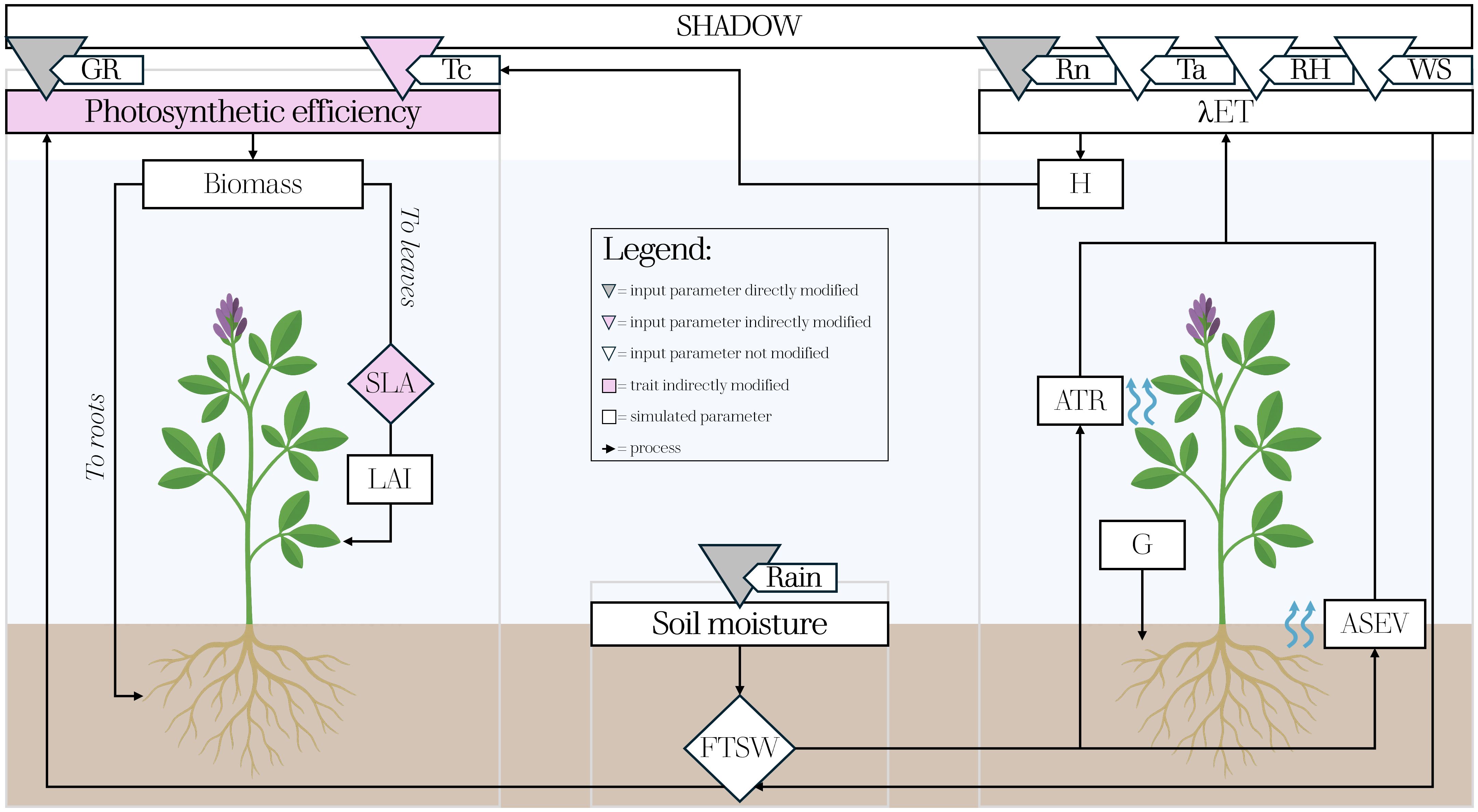
Figure 3. Simplified diagram of the crop modelling framework developed for assessing Alfalfa growth under different AVS. Grey, pink and white triangles indicate model input parameters directly, indirectly and not modified by shading effects, respectively. The remaining pink elements refer to morpho-physiological traits indirectly modified, while the white ones represent the parameters simulated by the model.

The basic structure of the model uses a process-based approach for hourly estimation of biomass accumulation (B_crop, g m^-2), which is dynamically partitioned to leaves, stems, and roots during the season. Accordingly, in non-limiting conditions (Equation 3):

$\begin{array}{ll}{B}_{crop} = fPAR ·I ·RUE& (3)\end{array}$

where I is the incident hourly global solar radiation (MJ m^-2) derived from the GroIMP radiation model, fPAR is the fraction of incident radiation intercepted by the canopy (unitless), and RUE is radiation use efficiency (g MJ^-1). $fPAR$ is calculated on an hourly time step according to Sinclair et al. (1992) (Equation 4):

$\begin{array}{ll}fPAR = 1- e^{[-LAI·\frac{k}{\sin (alpha)}]}& (4)\end{array}$

where k is the extinction coefficient of light in the canopy, and alpha (°) is the angle of sun elevation provided to the growth model by the GroIMP simulation of the daily course of solar track (section 2.3.2). RUE is calculated according to Yin et al. (2021), who modelled the canopy light use efficiency of C3 crops (${\Phi }_{CO2canopy}$, mol CO₂ mol^-1 photon) as (Equation 5):

$\begin{array}{ll}{\Phi }_{CO2canopy} = \frac{(C_c - {\Gamma }_{*}) · {\varphi }_{2LL}}{4·(C_c + 2{\Gamma }_{*})·(1 + {\varphi }_{2LL} + \frac{{\varphi }_{2LL} · k· I_{inc}}{J_{max}})}& (5)\end{array}$

where C_C is the chloroplast CO₂ level (μmol mol⁻¹), Γ_* is the CO₂ compensation point (μmol mol⁻¹), Φ_2LL is the electron transport efficiency of Photosystem II under limiting light (mol mol^-1), I_inc is incident light photosynthetically active radiation (PAR, μmol m⁻² s⁻¹), and J_max is canopy-top leaf maximum electron transport rate under light-saturating conditions (μmol e⁻ m⁻² s⁻¹). Further description of the functional formulations related to temperature sensitivity of Γ_* and J_max, as well as the nitrogen-dependent scaling of J_max for photosynthetic response, is provided in SI (Supplementary Figure S2). The parametrization of the alfalfa growth model is provided in Table S1.

Canopy light use efficiency (CO2_,canopy), calculated in not limiting water conditions, is then converted into RUE according to van Oijen et al. (2004) and Yin et al. (2021) (Equation 6):

$\begin{array}{ll}RUE = {\Phi }_{CO2,canopy} ·MM· (1 -\frac{R}{P}) ·4.56 ·\frac{0.5}{C_{biom}}& (6)\end{array}$

where R/P (crop respiration-to-photosynthesis ratio) was set to 0.4 (Yin et al., 2021); MM (the molar mass of carbon) was fixed at 12 g mol⁻¹ and a conversion factor of 4.56 was used to translate photosynthetically active radiation (PAR) from MJ to moles of photons, assuming that PAR represents 50% of incoming global solar radiation. The carbon fraction in crop biomass (C_biom) was set to 0.48.

Assimilated biomass at the hourly scale is accumulated daily and partitioned to the different organs according to dynamic partitioning coefficients (PCs, ratio), which are dependent on photoperiod (PP, hours) as provided by the radiative model of GroIMP. Specifically, for PP before the spring equinox, PC to above ground biomass (AGB, g m^-2) (i.e., leaves and shoots) is set to 0.9 while it decreases to 0.67 between the equinox and summer solstice (Brown et al., 2006). After that, as PP starts decreasing, PC to AGB drops to 0.35, considering that at the end of the season, the plant improves the accumulation of reserve substances in the roots to ensure vegetative recovery after the winter (Teixeira et al., 2007). According to Brown et al. (2006), this stage was assumed to start when PP decreases to 1h less than the daylength at solstice.

Biomass partitioned to AGB is further partitioned to leaves (PC_leaf) (Equation 7) and shoots (PC_shoots) (Equation 8) according to an allometric equation that assumes an exponential decrease in PC_leaves as increased dry matter to AGB (Brown et al., 2006; Teixeira et al., 2009). Accordingly:

$\begin{array}{ll}P{C}_{leaf} = c · exp\left(\frac{d}{AGB {10}^{-2} + e}\right)& (7)\end{array}$

$\begin{array}{ll}P{C}_{shoots} = 1- P{C}_{leaves} & (8)\end{array}$

where c, d and e are empirical coefficients shaping the response of PC to leaves to AGB (Supplementary Table S1).

The biomass partitioned to leaves (g m^-2) is converted into new leaf area (LAI_rate, m² m^-2) considering biomass investment per unit leaf area (Specific Leaf Area, SLA, m² g^-1) (Equation 9).

$\begin{array}{ll}LAIrat{e}_{(t)}=AGB·P{C}_{leaves} ·SLA& (9)\end{array}$

On the evidence that plants show an increase in SLA as an adaptation to shading conditions, as observed in the literature (Scarano et al., 2024; Potenza et al., 2022; Evans, 2001) and the experiment in Site B (Moretta et al., 2025), SLA was dynamically modified over each tile by quantifying the relevant degree of shading. Accordingly, a shadow factor (ShF, unitless) is calculated as the ratio between incoming global radiation (GR) and that intercepted by each tile (I), which ranges between 1, when the radiation intercepted by the tile corresponds to the external global radiation (no shadow), up to 0, corresponding to a complete shadowing (Equation 10):

$\begin{array}{ll}ShF = \frac{I}{GR}& (10)\end{array}$

The shadow effect on SLA is assumed for ShF lower than 0.9, where the increase in SLA was calculated as (Equation 11):

$\begin{array}{ll}incSLA = SLAmax·(1 -ShF) & (11)\end{array}$

where $SLAmax$ represents the maximum increment of SLA in response to a complete shadowing according to the results obtained in Site B (0.25; Moretta et al., 2025). inc_SLA, calculated on an hourly basis for each tile, is daily averaged and finally used to update the original SLA and the relevant LAIrate.

The simulation of LAI is completed by the simulation of leaf area senescent rate (SENrate, m² m^-2) (Equation 12) that is modelled by assuming a fixed senescence rate (FixSENrate, m² m^-2) multiplied by a Stage Factor (SF, unitless), a Cover Factor (CF, unitless), a Temperature Factor (TF, unitless), and a Water Stress Factor (WSF, unitless) (Yang et al., 2022).

SF starts linearly increasing from active vegetative growth (SF = 0) to floral buds’ visible stage (BV) (SF = 0.3). This stage is dependent on daily mean temperature (Tmean,°C) and PP, where the attainment of the phase, in the original configuration of Teixeira et al. (2011), is determined by an accumulation of 700 degree days (DDA,°C) (base temperature Tb=0°C) at PP = 10h, linearly decreasing up to 270 DDA at PP>14h condition. After BV, temperature becomes the primary driver of anthesis, defined as the stage when 50% of stems have open flowers. This is initially set to occur at 274 DDA after BV, corresponding to SF = 0.6, which increases to 1 in the following stage (grain filling).

CF increases linearly from 0 to 0.5 as LAI increases from 2 to 4, and then continues to increase, reaching a maximum value of 1.5 at LAI 7.

TF is set to 0.1 for mean daily temperatures between 0 and 5°C, then increases progressively, reaching 1 at 20°C, and peaking at a maximum of 1.5 at 40°C.

WSF is assigned a value of 1 when the Fraction of Transpirable Soil Water (FTSW) is greater than 0.5. Below this threshold, WSF increases linearly up to 2 as FTSW decreases down to the wilting point (FTSW = 0.1).

Accordingly:

$\begin{array}{ll}SENrat{e}_{(t)}=FixSENrate·SF·CF·TF·WSF& (12)\end{array}$

LAI at time t is then updated (Equation 13):

$\begin{array}{ll}LA{I}_{(t)}=LA{I}_{(t-1)}+LAIrat{e}_{(t)}-SENrat{e}_{(t)}& (13)\end{array}$

A soil water balance module is integrated to simulate water limitation experienced by the canopy during the growing season and the relevant impact on plant transpiration and photosynthesis. The soil water balance is calculated for a single layer where the total transpirable soil water (TTSW, cm) is estimated considering the water content availability (WCA, cm cm^-1) between field capacity and wilting point and the root depth (cm). Assuming no surface runoff, available soil water for the layer (ATSW_d, cm) depends on the ATSW of the previous day (ATSW_d-1, cm), and the positive (rainfall and/or irrigation, mm) and negative contribution (actual evapotranspiration, ET, mm) to the water budget (Equation 14).

$\begin{array}{ll}ATS{W}_d=ATS{W}_{(d-1)}+ (Rainfal{l}_{(d)}+Irrigatio{n}_{(d)})-E{T}_{(d)}& (14)\end{array}$

where rainfall, irrigation and ET are converted from mm to cm.

The calculation of actual evapotranspiration ET is preceded by the estimation of potential evapotranspiration (PET, mm), that representing the atmospheric evaporative demand under non-limiting water conditions, serves as a reference for deriving ET by incorporating constraints related to soil water availability and crop-specific stress factors. PET is calculated according to Penman-Monteith approach at hourly timestep (Equation 15):

$\begin{array}{ll}PET= \frac{(\Delta (R_n-G)+{\rho }_a{c}_p\frac{(e_s-e_a)}{r_a})}{(\Delta +\gamma (1+\frac{r_s}{r_a}))}{\lambda }^{-1}& (15)\end{array}$

where λ is the latent heat of vaporization (J Kg^-1), Rn is the net radiation (Wm^-2), G is the soil heat flux (Wm^-2), (e_s-e_a) represents the vapour pressure deficit of the air (VPD, KPa), ρ_a is the mean air density at constant pressure (Kg m^-3), c_p is the specific heat of the air (J K^-1m^-3), Δ is the slope of the saturation vapour pressure temperature relationship (KPa°C^-1), γ is the psychrometric constant (KPa°C^-1), and r_s and r_a are the surface and aerodynamic resistances (s m^-1).

Considering that Rn, G, and VPD data were not available at the experiment sites, they were calculated according to Allen et al. (1998). Hourly net radiation Rn was calculated as the difference between net shortwave radiation (Rns) and net longwave radiation (Rnl). Rns were obtained by correcting incoming solar radiation for surface albedo (assumed 0.23), while Rnl was estimated using the Stefan-Boltzmann law based on hourly air temperature, vapor pressure, and the ratio of measured to clear-sky solar radiation. G was calculated as 10% Rn during the day, to 50% at night. Hourly vapor pressure deficit (VPD) was calculated as the difference between saturated vapor pressure, derived from air temperature, and actual vapor pressure, estimated from observed relative humidity. For more comprehensive information, we recommend consulting the original publication.

Surface resistance (rs) was assumed to be 70 s m^-1 during the day (Allen et al., 1998) and 700 s m^-1 during the night (e.g. Meyers and Hollinger, 2004) to account for stomatal closure when radiation is missing.

Aerodynamic resistances ra is calculated according to Thom and Olivier (1977) as (Equation 16):

$\begin{array}{ll}{r}_a=\frac{[4.72·[ln((z-d+z_o)/z_o{]}^2]}{( 1+0.54·u)}& (16)\end{array}$

where u is wind speed (ms^-1) at reference height z (2 m), d is the zero-displacement height equal to 1.04 h^0.88 and z₀ the roughness length for momentum and heat transfer equal to 0.062 h^1.08, where h is the crop height, assumed as a function of accumulated AGB according to a logistic function (SI).

PET is partitioned between plant transpiration and soil evaporation that are then rescaled to the relevant actual values considering the limitations imposed by current water conditions. $fPAR$ is used as a scalar to partition ET between soil and crop, where the proportion of PET allocated to potential transpiration is $fPAR$ and that to potential soil evaporation is 1- $fPAR$ (Marsal et al., 2014). Potential transpiration is rescaled to actual transpiration considering that plant’s gas exchange is regulated by the extractable soil water content, expressed by the ratio between ATSW and TTSW (i.e., fraction of transpirable soil water, FTSW, unitless; Sinclair and Muchow, 1999) (Equation 17).

$\begin{array}{ll}RelTr= {(1+a·exp(b·FTSW))}^{-1}& (17)\end{array}$

where $RelTr$ is the fraction of actual to potential transpiration (ranging from 1, when FTSW is not yet limiting potential transpiration, to 0, where FTSW completely inhibits transpiration), and a and b are empirical parameters shaping the response of RelTr to FTSW. The RelTr is also used to rescale the potential RUE (Equation 6) to its actual value by considering that the reduction in RUE is directly proportional to the reduction in transpiration (Sinclair and Muchow, 1999; Supplementary Figure S4).

Similarly, a rescaling factor for soil evaporation (RedEvap) is calculated when soil moisture diverges from a condition equivalent to that of a wet surface, assumed when FTSW>0.5 (Soltani and Sinclair, 2012). RedEvap is thus calculated as a function of the square root of time (DYSE, days) since FTSW is lower than 0.5 (Equation 18):

$\begin{array}{ll}RedEvap=[{(DYSE+1)}^{0.5}-{(DYSE)}^{0.5}]& (18)\end{array}$

Finally, actual transpiration (ATR, mm) (Equation 19) and soil evaporation (ASEV; mm) (Equation 20) are calculated as:

$\begin{array}{ll}ATR = fPAR · PET·Kc · RelTr& (19)\end{array}$

$\begin{array}{ll}ASEV = (1-fPAR)· PET·Kc · RelEvap& (20)\end{array}$

where Kc is the crop coefficient, assumed constant (1.05) during the growing season (Allen, 1996).

Considering that the hourly energy balance is calculated as (Equation 21):

$\begin{array}{ll}{R}_n=G+H+ \lambda ET& (21)\end{array}$

where Rn and G are known terms and actual λET may be calculated as the sum of ATR and ASEV and then converted via $\lambda$, the sensible heat H (Wm^-2) may be derived as difference and used to calculate the hourly temperature of the canopy (Tc,°C), accounting for the effect of a reduced transpiration on plant temperature (Webber et al., 2018). The Tc (Equation 22) is then introduced as a factor affecting photosynthetic efficiency (Γ_* and J_max, SI).

$\begin{array}{ll}{T}_c=T_a+\left(\frac{H·ra }{{\rho }_a·c_p}\right)& (22)\end{array}$

By embedding the crop growth model within the same platform as the radiative model in GroIMP, the framework dynamically accounts not only for the effect of absorbed global radiation and PP on plant growth and development but also for the impact of photovoltaic panels water harvesting its subsequent redistribution to the ground area immediately below their slopes. Accordingly, rainfall intercepted by the photovoltaic panels is redistributed onto the ground within the first meter linearly extending from the lower edge of the panels (Moretta et al., 2025) (Equation 23):

$\begin{array}{ll}{R}_a=R_m+R_i& (23)\end{array}$

where $R_a$is the total daily cumulated total rainfall (mm), including daily measured rainfall ($R_m$) and that intercepted by the panel ($R_i$) that is calculated according to (Equation 24):

$\begin{array}{ll}{R}_i=R_m·A_{panel}·Rc& (24)\end{array}$

where $A_{panel}$ is the effective collecting area calculated per linear meter of panel and Rc is the precipitation runoff conversion coefficient. In this study, Rc was set to 0.9 (90%). $A_{panel}$ is calculated as (Equation 25):

$\begin{array}{ll}{A}_{panel}=Length · Width · \cos (\alpha )& (25)\end{array}$

where Length is the length of the panel (m), Width is the width of the panel (m) and $\alpha$ is the tilt angle of the panel relative to the ground norm.

Conversely, the water input below the area under the panels’ projection was considered negligible in all cases. In this context, a 1.5 m strip on both sides of each supporting pole, representing the area most influenced by potential rainfall shielding and runoff from the panels, was excluded from the computation domain.

Considering the simplified structure of the model, model calibration was limited to the tuning of a limited subset of parameters, while core physiological and structural parameters remained fixed, as they were derived from experimentally validated sources. Specifically, the calibration considered coefficients and timing of PC to above/below ground biomass as these parameters determine the accumulation and subsequent distribution of biomass in the leaves and stem. In addition, the flowering period was considered, as it plays a key role in driving leaf surface senescence.

As such, the model was initially applied over the calibration sites for testing LAI and biomass accumulation (Site A) and phenology (Site B) considering the initial parameterization for phenology and biomass partitioning in accordance with the literature data (Supplementary Table S1). As a second step, based on the model’s performance, the relevant parameters were modified to adjust the model’s performance to the observed results.

To further explore the interaction between crop growth, water regime and energy production, the calibrated model was used to perform additional simulations (Site C; 2024) varying the pitch distance (spacing between PV panel rows) from 4 m to 16 m every 2m. For each configuration we calculated the relative alfalfa yield of three harvests and the relative PV energy production were calculated, both under non-limiting and water-limiting conditions (50 % reduction in seasonal rainfall).

2.4 Statistical analysis

To assess the performance of the integrated modeling framework in simulating alfalfa above ground biomass, LAI, and canopy temperature under different AVS configurations, a set of standard statistical indicators was employed. These included the Root Mean Square Error (RMSE), the Mean Bias Error (MBE), and the coefficient of determination (R²). In addition to these performance metrics, the Akaike Information Criterion (AIC) was calculated to evaluate the trade-off between model accuracy and complexity.

Statistical comparisons between shading treatments were performed using analysis of variance (ANOVA), followed by Tukey’s Honest Significant Difference (HSD) post-hoc test to identify differences in biomass accumulation and LAI across spatial positions. For variables measured repeatedly on the same plots across multiple sampling dates, a repeated-measures ANOVA was applied to account for temporal autocorrelation. Normality and homogeneity of variances were tested using the Shapiro–Wilk and Levene’s tests, respectively. All statistical analyses were conducted using R software (version 4.4.3; R Core Team, 2025), and significance was accepted at p < 0.05 unless otherwise stated.

3 Results

3.1 Model calibration

Under the initial configuration (Supplementary Table S1), the model slightly underestimated the DOY of full anthesis recorded in Site B in both 2023 and 2024. In 2023 the first flowering date was recorded on DOY 135 and the second, after the first mowing, on DOY 197, which were simulated respectively on DOY 130 and 190. In 2024, the flowering date was recorded on DOY 186, as the earlier cuts prevented reaching this stage previously and simulated on DOY 180. Accordingly, the thermal time from the bud visible stage to full anthesis was increased from its original value (270 degree-days) to 310 degree-days, resulting in a simulated flowering date within ±1 day of the observed DOY.

Under this configuration, the model was tested in Site A (2019), under open field conditions. In this experimental site, alfalfa showed an observed cumulative production of approximately 1,250 g m^-2 (12.5 t ha^-1) at the end of the 2019 season. The three growing cycles, separated by mowing at DOY 153, 211 and 240, produced about 500, 420 and 330 g m^-2, respectively. The LAI peaked at about 5.1 m² m^-2 before the first mowing, followed by decreasing values and subsequent recoveries with peaks of 3.2 and 2.8 m² m^-2 in subsequent cycles. The model well reproduced the growth dynamics of both biomass and LAI for the first two mowings (Figure 4), highlighting the overall consistency of the proposed approach in simulating the process of biomass accumulation and partitioning and the senescence. Conversely, the model failed to adequately capture the regrowth dynamics following the second harvest during the terminal phase of the growing season (Figure 4) highlighting a potential inconsistency in the parameterization that defines the period during which biomass is preferentially allocated to the roots (i.e. at the end of growing season), as well as in the associated partitioning coefficient. In terms of predictive performance, the model yielded R² = 0.82, RMSE = 48.6 g m⁻², MBE = 12.1 g m⁻², and AIC = 125.4 for biomass, and R² = 0.74, RMSE = 0.62, MBE = 0.18, and AIC = 92.7 for LAI in this pre-calibration phase.

Figure 4

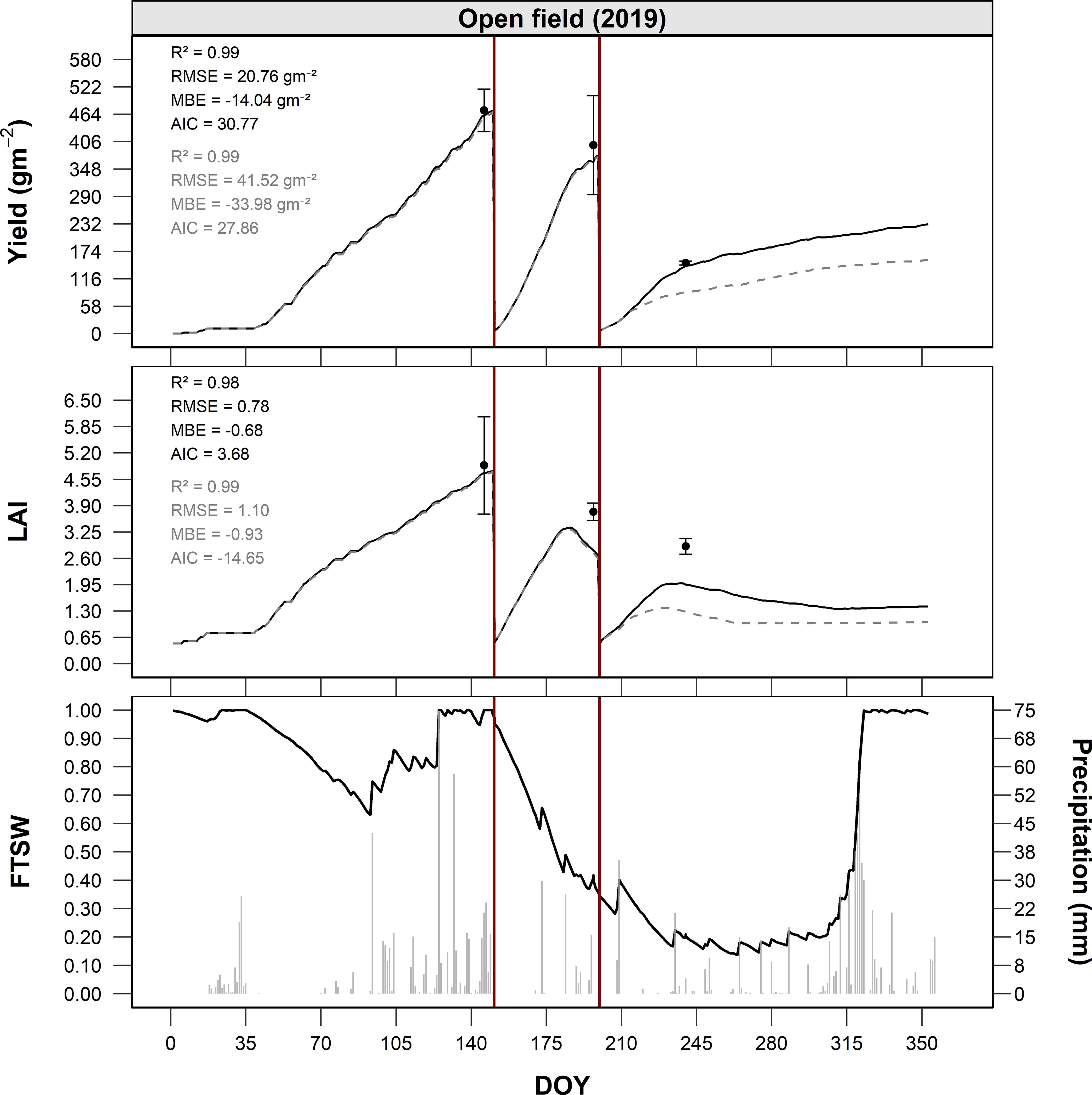
Figure 4. Seasonal dynamics of yield (g m^-2), LAI (m² m^-2), and FTSW under open-field (Site A) conditions in 2019, as a function of DOY. Post-calibration simulations are shown as black solid lines, while pre-calibration simulations are represented by grey dashed lines. Observed data are indicated by points with error bars. The bottom panel illustrates the seasonal course of FTSW (black solid line) together with daily precipitation (grey columns). Vertical red lines indicate dates of full-field harvest.

Accordingly, the PP triggering this shift under shortening day length conditions, was tuned in a range -1h (original value) to -2h with respect to the solstice (step 0.5h), considering all possible combinations with PC to AGB in the range between 0.35 (original value) and 0.5 (step 0.05). Finally, the best combination PP-PC providing the best performance in simulating biomass and LAI was selected.

Quantitative assessment of model performances after this second step improved model performances for both total biomass and LAI predictions. After calibration, the model achieved an R² of 0.99, RMSE of 20.76 g m^-2, MBE of -14.04 g m^-2, and AIC of 30.77 for total biomass. For LAI, the model reached an R² of 0.98, RMSE of 0.78, MBE of -0.68, and AIC of 3.68, indicating a substantial enhancement in accuracy and precision compared to the pre-calibration phase.

3.2 Fixed agrivoltaic system

The performance of the calibrated model was evaluated at the fixed AVS (Site B) by comparing simulated and observed dry matter yield of alfalfa under four treatments (TR1-TR4, Supplementary Table S2) during the 2023 and 2024 growing seasons.

In 2023 (Figure 5), observed biomass accumulation revealed a clear gradient among treatments: TR1 achieved the highest yields, likely due to increased soil moisture availability from panel-induced runoff, followed by TR2, while TR3 and TR4, located in more heavily shaded areas, showed substantially lower productivity. Before the first cut (DOY 153), TR1 reached approximately 580 g m⁻², TR2–510 g m⁻², TR3–260 g m⁻², and TR4 only 120 g m⁻². After the second growth phase (DOY 240), cumulative yields increased to approximately 1,050 g m⁻² for TR1, 900 g m⁻² for TR2, 560 g m⁻² for TR3, and 290 g m⁻² for TR4. By the end of the season, total annual yields were approximately 1,350 g m⁻² for TR1, 1,150 g m⁻² for TR2, 700 g m⁻² for TR3, and 400 g m⁻² for TR4. Using TR2 as a reference, this corresponds to a +17.4% increase in TR1, and reductions of -39.1% and -65.2% for TR3 and TR4, respectively. The agreement between observed and simulated values was good (R² = 0.83, RMSE = 56.6 g m⁻², MBE = -23.1 g m⁻²).

Figure 5

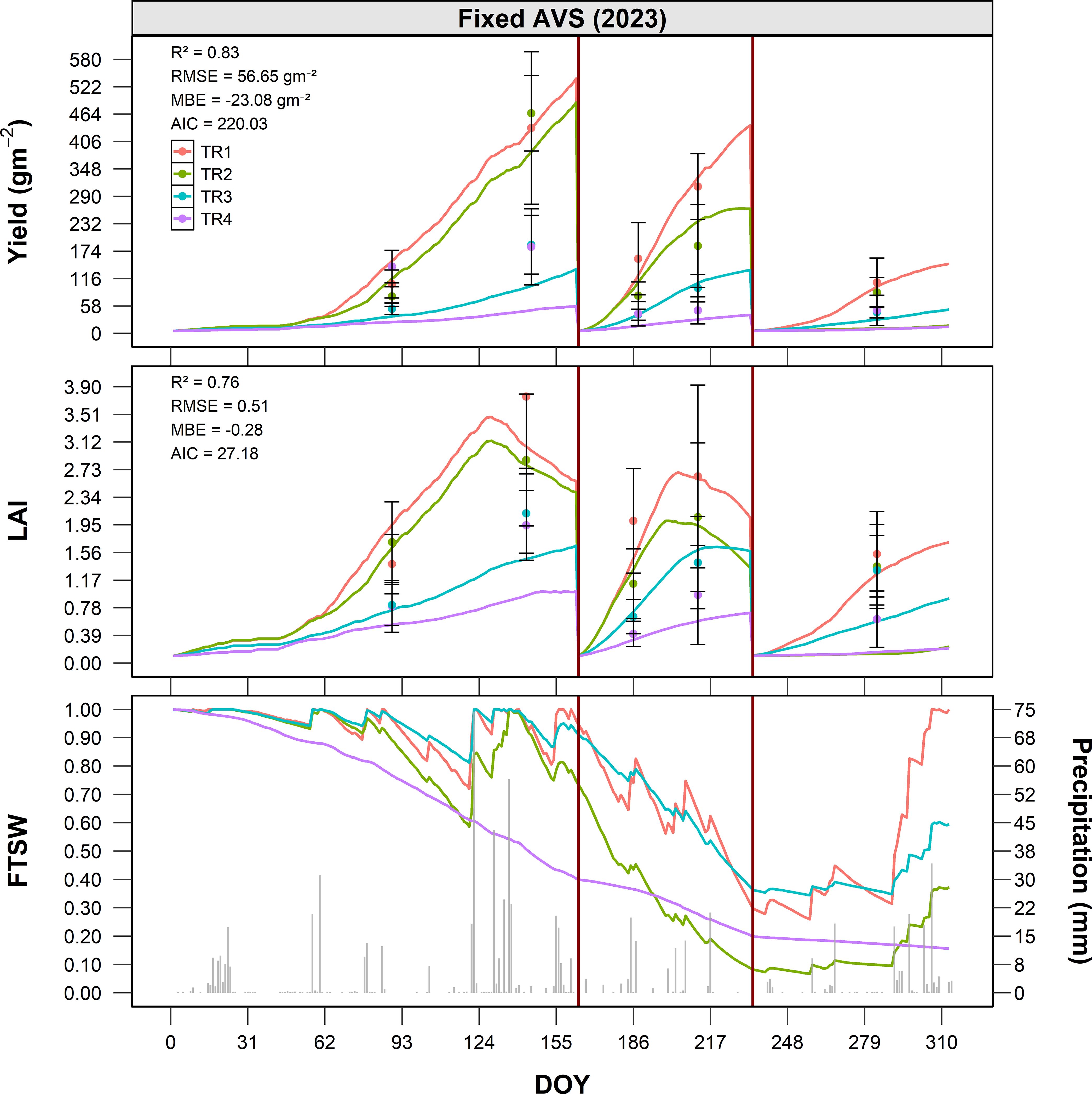
Figure 5. Seasonal dynamics of alfalfa dry matter yield (g m^-2), LAI (m² m^-2), and FTSW under fixed AVS conditions (Site B) in 2023, as a function of DOY. Simulated values are shown as solid lines for four treatments (TR1–TR4), while observed data are represented by points with error bars (mean ± standard error). The bottom panel illustrates the seasonal course of FTSW (solid lines) together with daily precipitation (grey columns). Vertical red lines indicate the dates of full-field harvest.

In 2024 (Figure 6), similar spatial patterns were observed, though overall yields were lower due to different climatic and management conditions, including a higher number of harvests. Before the first cut (DOY 122), TR1 reached approximately 230 g m⁻², TR2–200 g m⁻², TR3–120 g m⁻², and TR4–80 g m⁻². After the second growth cycle (DOY 211), yields were around 460 g m⁻² for TR1, 360 g m⁻² for TR2, 260 g m⁻² for TR3, and 160 g m⁻² for TR4. At the end of the season (DOY 268), cumulative yields were approximately 650 g m⁻² for TR1, 520 g m⁻² for TR2, 390 g m⁻² for TR3, and 280 g m⁻² for TR4. Compared to TR2, this corresponds to a +25.0% increase in TR1, and reductions of -25.0% and -46.2% for TR3 and TR4, respectively. The model accurately reproduced treatment-based differences in productivity, with overall satisfactory performance also in 2024 (R² = 0.85, RMSE = 41.4 g m⁻², MBE = 9.6 g m⁻²), confirming the robustness of the approach for simulating spatially heterogeneous AVS.

Figure 6

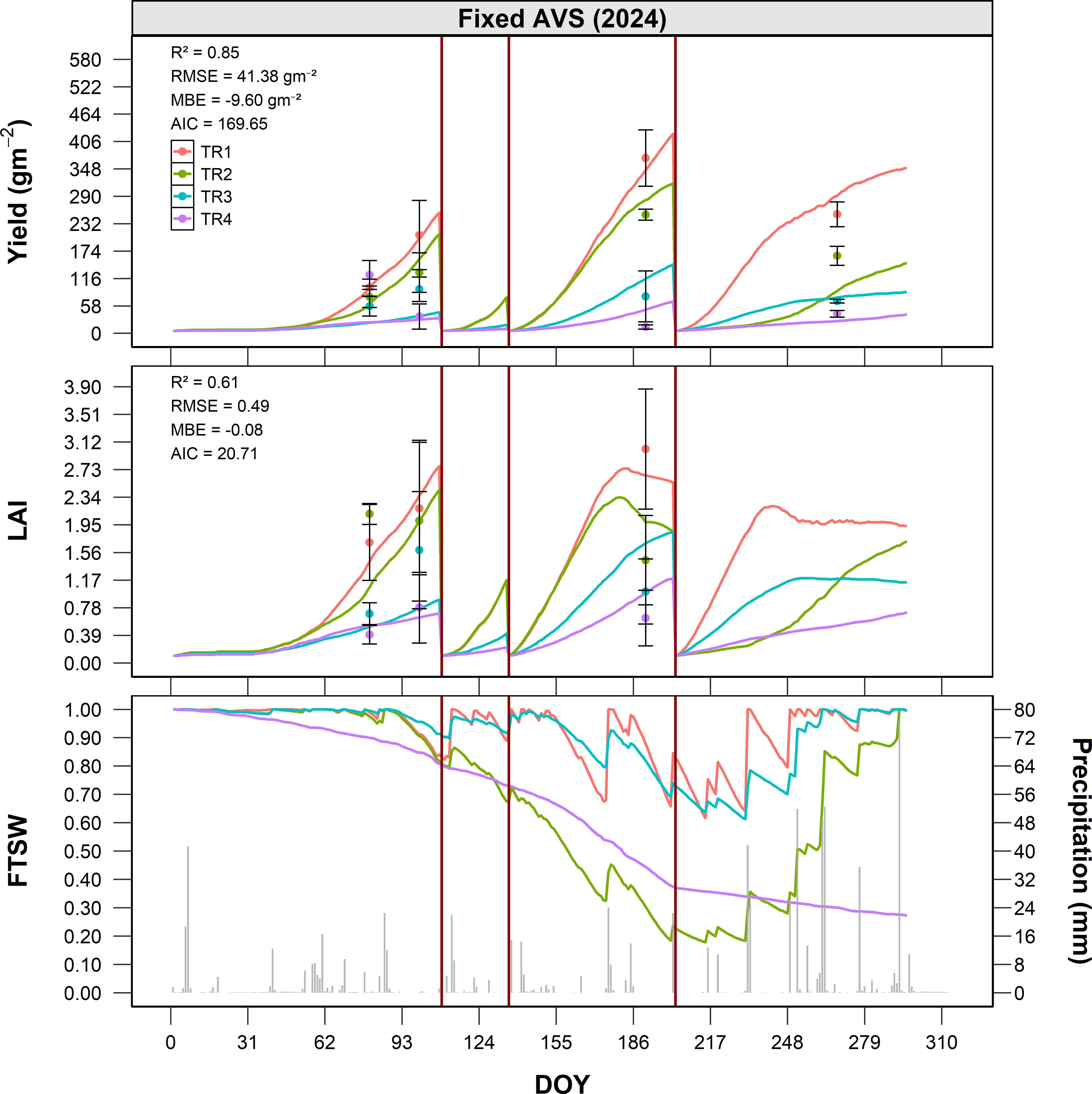
Figure 6. Seasonal dynamics of alfalfa dry matter yield (g m^-2), LAI (m² m^-2), and FTSW under fixed AVS conditions (Site B) in 2024, as a function of DOY. Simulated values are shown as solid lines for four treatments (TR1–TR4), while observed data are represented by points with error bars (mean ± standard error). The bottom panel illustrates the seasonal course of FTSW (solid lines) together with daily precipitation (grey columns). Vertical red lines indicate the dates of full-field harvest.

The simulation of FTSW in 2023 revealed pronounced differences among treatments, reflecting their spatial arrangement within the fixed AVS (Figure 5). TR1 consistently maintained the highest FTSW values, remaining above 0.6 for most of the season, supported by localized water redistribution from the northern panel edge. TR2 exhibited a steeper decline after the first harvest, with values approaching 0.5 by mid-season, indicating a faster depletion of soil water. TR3 and TR4, located beneath the panels and with limited direct access to rainfall (particularly TR4), showed the lowest soil moisture availability. In both treatments, FTSW dropped below 0.4 during the central part of the growing season (DOY 150–240), confirming greater exposure to water stress.

In 2024, FTSW dynamics followed a similar spatial gradient, but with overall higher values across all treatments, mainly due to more frequent rainfall events recorded during the summer period (DOY 160–240). Consequently, differences among treatments were less pronounced than in 2023. TR1 again maintained the highest FTSW, although the gap with TR2 and TR3 was reduced. TR4 remained the lowest, but without the sharp decline observed in the previous year.

3.3 Bi-axial agrivoltaic system

The performance of the calibrated model was evaluated under bi-axial AVS (Site C) conditions during the 2024 growing season. Figure 7 compares simulated and observed dry matter yield for four treatments (TR1 to TR4), corresponding to different shading levels and spatial positions relative to the solar panel configuration (Supplementary Table S2). The model demonstrated strong predictive accuracy, with a R² of 0.94, RMSE of 39.3 g m^-2, and an MBE of -3.4 g m^-2, indicating a slight overestimation of yield.

Figure 7

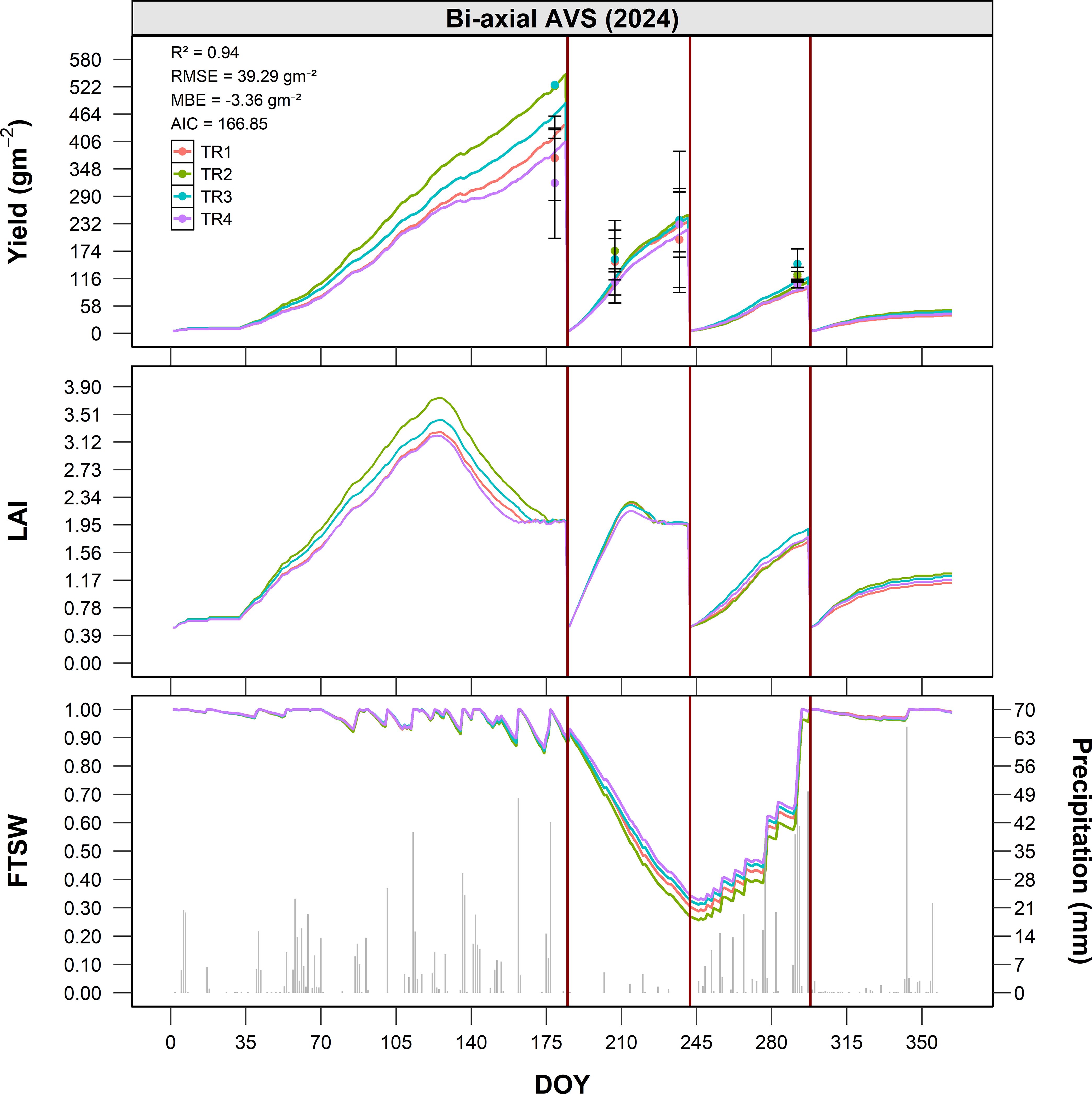
Figure 7. Seasonal dynamics of alfalfa dry matter yield (g m^-2), LAI (m² m^-2), and FTSW under bi-axial AVS conditions (Site C) in 2024, as a function of DOY. Simulated values are shown as solid lines for four treatments (TR1–TR4), while observed data are represented by points with error bars (mean ± standard error). The bottom panel illustrates the seasonal course of FTSW (solid lines) together with daily precipitation (grey columns). Vertical red lines indicate the dates of full-field harvest.

During the first growth phase (DOY 66-182), TR2 exhibited the highest productivity, reaching approximately 550 g m^-2, followed by TR3 and TR1, with yields around 500–520 g m^-2. TR4 consistently recorded the lowest yield (~470 g m^-2), reflecting a reduction of about 15% compared to TR2. These results highlight the significant influence of spatial positioning and light availability under biaxial tracking systems on biomass accumulation.

In the second regrowth phase (DOY 182-240), TR2 again showed the most vigorous recovery, followed by TR3, TR1, and TR4. Yield differences among treatments remained consistent, with TR4 accumulating approximately 10–15% less biomass than the most productive treatment.

During the final growth phase (DOY 240-298), yield levels among TR1, T2, TR3, and TR4 converged, suggesting a reduced marginal impact of partial shading under late-season conditions. Nonetheless, TR4 maintained a slightly lower cumulative yield, ending the season with approximately 10% less biomass than TR2, reinforcing the adverse effects of sustained shading on alfalfa productivity. Considering the annual cumulative biomass production averaged over harvests, alfalfa grown in Site A (open field, 2019) recorded the highest mean yields. The bi-axial tracking AVS (Site C, 2024) achieved a comparable annual output, remaining generally within about 10 % of the open-field reference. In the fixed-panel AVS (Site B, 2023–2024), when the calculation is restricted to the pre-existing, less shaded corridors (i.e., the productive inter-row areas comparable to TR1 and TR2), the system reached roughly 70 % of open-field alfalfa productivity on an annual basis. In contrast, the persistently shaded corridors contributed negligibly to yearly biomass and would scarcely justify cultivation.

The FTSW simulations show a very similar trend among the four treatments, with no marked differences related to the position with respect to the photovoltaic modules. During the first growth phase, the values remain close to 1, indicating optimal water availability. In the middle of the season (DOY 182-280), a progressive reduction in FTSW is observed, with minimums around 0.3-0.4, consistent with moderate but uniform water stress conditions across the plots. Starting from DOY 280, the recovery of rainfall causes a rapid rise in FTSW towards values close to saturation, restoring conditions that do not limit growth.

3.3.1 Canopy temperature simulation

The simulation of canopy temperature was evaluated at Site C (bi-axial AVS) across four spatial positions (TR1 to TR4) during the 2024 growing season (Figure 8). Observed canopy temperature dynamics varied across treatments and dates, reflecting both spatial heterogeneity and seasonal changes. Canopy temperatures exhibited a clear seasonal trajectory, increasing progressively from early measurements (DOY 183) to a peak during mid-season (DOY 241), followed by a marked decline by late season (DOY 296). Across all sampling dates, the highest temperatures were consistently recorded in the central treatments (TR2 and TR3), which correspond to the areas with the lowest shading levels. The model successfully captured observed trends, including the progressive temperature gradient from heavily shaded (TR1 and TR4) to less shaded areas (TR2 and TR3). On all sampling dates, TR1 and TR4 consistently exhibited lower average canopy temperatures than TR2 and TR3, with the differences being most pronounced at mid-season (DOY 207 and 241). Simulated temperatures closely matched observed data, with slight overestimation in late-season measurements (DOY 296) particularly under TR1. Overall model performance was strong, with a coefficient of determination (R²) of 0.96 and a low RMSE of 0.87°C, confirming the accuracy of the simulation in reproducing observed canopy temperature across treatments.

Figure 8

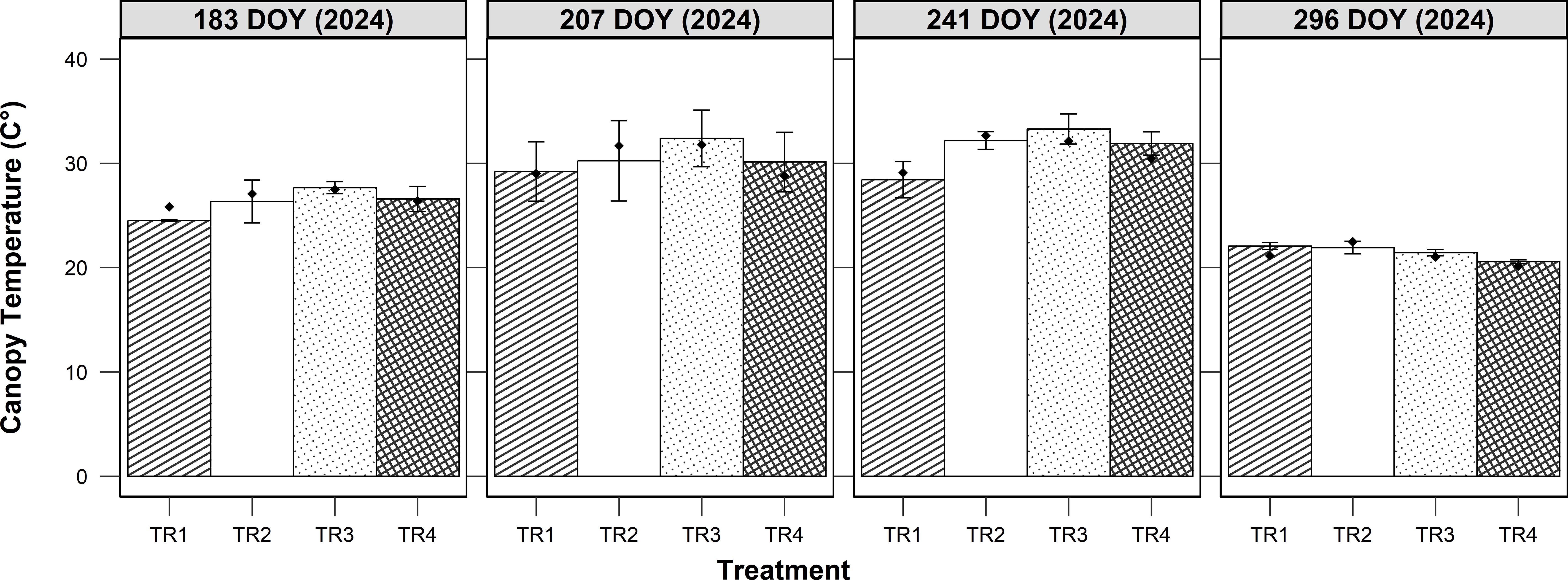
Figure 8. Observed and simulated canopy temperature (°C) for four treatments (TR1-TR4) across four dates (DOY 183, 207, 241, 296) at Site C. Columns show observed means with error bars (mean ± SE), while points represent simulated values.

To assess treatment effects on crop microclimate, canopy temperature was measured and expressed as the difference between canopy and air temperature (ΔT = canopy temperature minus air temperature) across four shading treatments (TR1 to TR4) and four sampling dates (DOY 183, 207, 241, and 296) at the Site C. Observed ΔT values showed clear differences among treatments and dates, reflecting variations in both shading intensity and environmental conditions. On days 207 and 241, corresponding to mid-summer conditions with air temperatures above 30°C, the largest temperature differences were recorded. The most shaded treatments (TR1 and TR4) consistently exhibited lower canopy temperatures than the least shaded ones (TR2 and TR3), with ΔT differences exceeding 3°C. On cooler days (183 and 296), when air temperatures were below 25°C, treatment differences were smaller but still evident. The model accurately reproduced these spatial and temporal patterns, showing good agreement with observed data (R² = 0.83, RMSE = 0.88°C, and MBE = - 0.11°C; Figure 9), confirming its effectiveness in simulating canopy thermal dynamics under variable shading conditions.

Figure 9

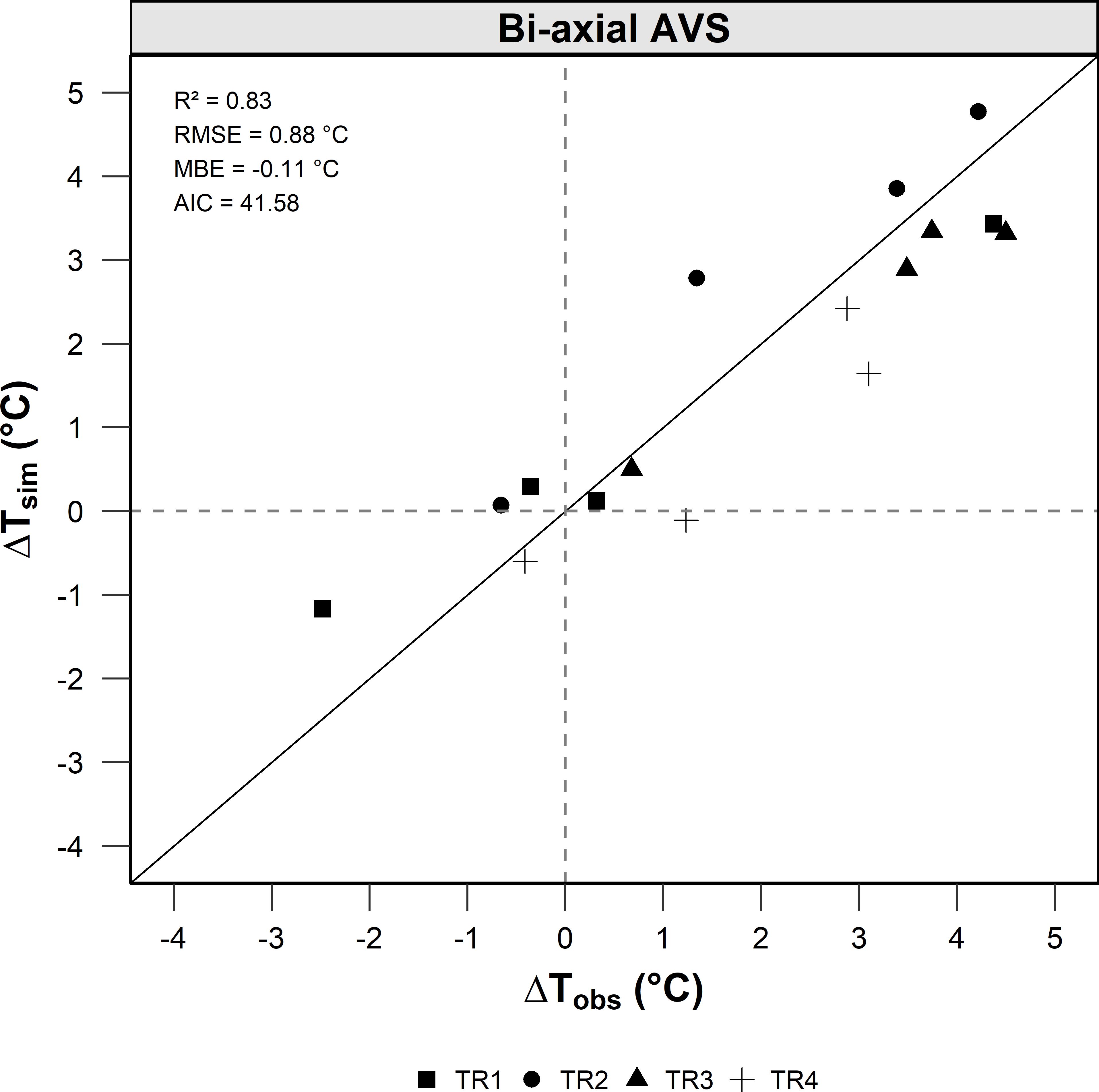
Figure 9. Comparison between simulated (ΔT_sim) and observed (ΔT_obs) canopy-to-air temperature difference (ΔT = T_canopy – T_air) across four shading treatments (TR1–TR4) under the bi-axial tracking agrivoltaic system (Site C) during the 2024 growing season.

3.4 Overall model performance in simulating biomass yield and LAI across AVS configurations

The accuracy of the integrated modeling framework was assessed by comparing simulated and observed values of yield (Yield_sim vs Yield_obs) and LAI (LAI_sim vs LAI_obs) across all experimental sites and treatments, including open field, fixed-panel AVS (Site B), and bi-axial tracking AVS (Site C).

As shown in Figure 10A, the model captured yield dynamics with high accuracy (R² = 0.94), with a RMSE of 110,34 g m^-2 and a MBE of –54.7 g m^-2, indicating a slight overall underestimation. The wide distribution of treatment-specific data points (TR1 to TR4) confirms the model’s robustness in representing productivity across a range of shading intensities and microclimatic conditions. The slight underestimation tendency is more evident under high-yielding conditions (>400 g m⁻²), where the model showed conservative predictions, likely due to limitations in simulating peak growth phases or resource-unlimited scenarios.

Figure 10

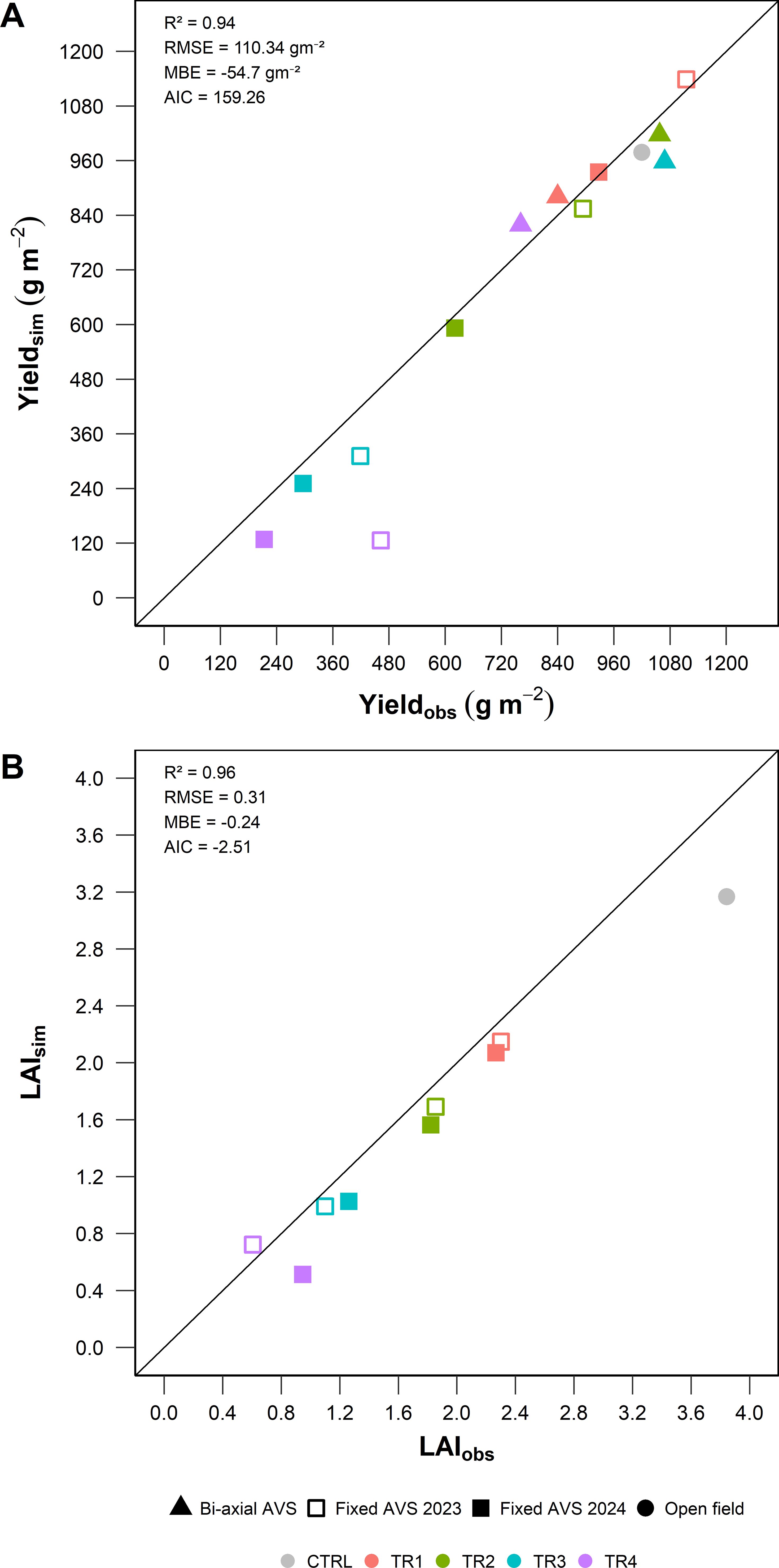
Figure 10. Comparison between simulated and observed values of (A) annual yield (sum per site and treatment) and (B) mean LAI at harvest. Data include open field (Site A), fixed AVS (Site B), and bi-axial AVS (Site C).

In Figure 10B, the model also accurately reproduced the seasonal dynamics of LAI, with a coefficient of determination of R² = 0.96, RMSE =-0.24. Most of the underestimation occurred at moderate to high LAI values (>3), suggesting that the model may slightly underestimate canopy expansion during the most favorable growth periods. Nevertheless, the model successfully represented the full range of LAI development across treatments, confirming its ability to capture both regrowth phases post-harvest and senescence-driven declines.

3.5 Scenario simulations on pitch distance and water availability

Yield and energy production were differently affected by pitch distance depending on water availability (Figure 11). In the absence of water limitations, the reduction in available radiation resulting from a smaller pitch progressively constrains production relative to open-field conditions. Yield penalties at 4 m pitch reached about –50 % for the first harvest, while the second and third harvests showed progressively smaller reductions. In contrast, energy production decreased almost linearly with pitch distance, as larger spacing lowers the installed PV capacity per hectare.

Figure 11

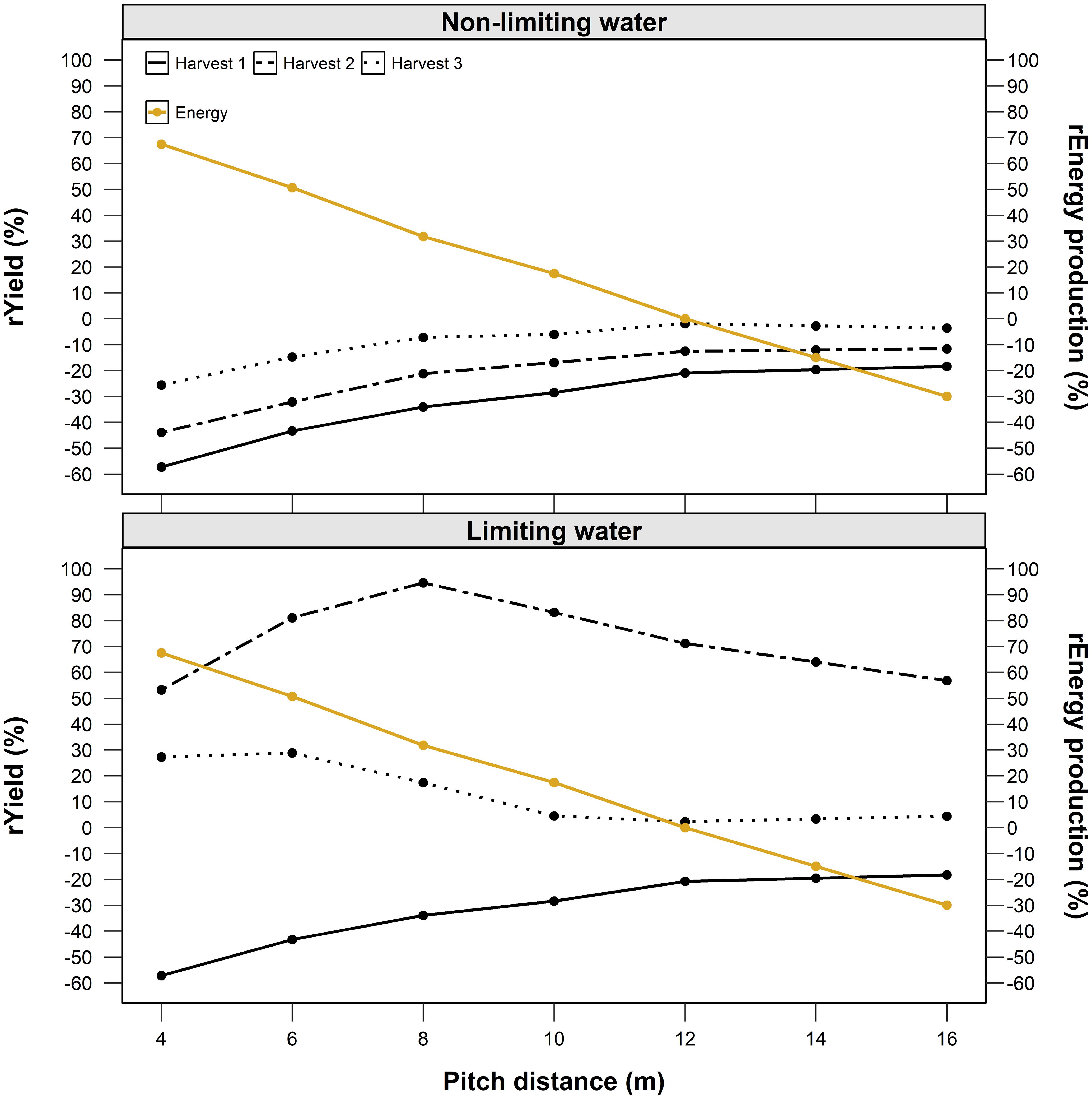
Figure 11. Modelled relative alfalfa yield of three harvests and PV energy production across pitch distances (4–16 m) under non-limiting (top) and water-limiting (bottom; 50 % rainfall) conditions.

Under water-limiting conditions, the response pattern changed. Moderate shading (pitch 6–8 m) mitigated drought stress with respect to open-field conditions by reducing canopy temperature and evapotranspiration, resulting in higher second-harvest yields than both narrower and wider layouts. The first harvest, when soil moisture was still adequate, and the third harvest, constrained by late-season stress, showed smaller differences among pitches. Energy production again declined with increasing pitch, but the agronomic advantage of intermediate spacing partly offset this loss.

4 Discussion

This study introduced a novel modeling framework based on the GroIMP platform that integrates a simplified, process-based crop growth model with a three-dimensional radiation environment. The proposed approach enabled an explicit, physics-based simulation of light transport, which successfully quantified radiation interception by the modeled elements (i.e., crop and panels). As highlighted in the literature (Zainali et al., 2025; Amaducci et al., 2018), most existing modeling platforms are not well-suited for AVS because they overlook the critical interaction between panel-induced shading and the morpho-physiological responses of cultivated plants. Such omissions can lead to significant biases in model predictions. To address this gap, our framework was designed to balance parsimony with the ability to capture essential plant-environment feedback. Specifically, it has been developed to simulate the effects of hourly dynamic shading on alfalfa, thereby providing a more accurate assessment of crop performance under AVS conditions.

In a recent study, Moretta et al. (2025) explored the impact of shading-induced microclimatic changes on alfalfa grown under the fixed AVS in Ravenna (Site B) by forcing the SSM crop model (Soltani and Sinclair, 2012) with image-derived fAPAR data, thereby circumventing the need to explicitly represent the morpho-physiological acclimation processes usually induced by reduced light availability. Conversely, the new prognostic approach presented here directly accounts for the physiological effects of lower radiation, providing a realistic simulation of alfalfa growth under shade that remains comparable to the forced SSM model.

In fact, the proposed framework incorporates key elements required to distinguish crop growth responses in shaded versus full-light conditions beneath PV panels. This integrated approach enables a more realistic simulation of the combined impacts of shading, drought and heat stress on plant morpho-physiological performance, which are especially critical in a Mediterranean climate where high temperature and low rainfall often limit plant growth during the season (Holmgren et al., 2012; Xu et al., 2020; Acevedo et al., 2024). The use of the GroIMP platform enabled the simulation of radiation dynamics at an hourly time step within a complex three-dimensional environment. This temporal resolution was crucial to capture the intra-daily variability of shading patterns induced by AVS structures. By explicitly representing these fluctuations, the model improved the realism of light–crop interactions. In contrast, many crop models commonly used to evaluate the effect of AVS on crop productivity such as STICS (Dupraz et al., 2011), EPIC (Campana et al., 2021) and APSIM (Ahmed et al., 2022), operate at a daily time step. While daily resolution is often sufficient to capture long-term growth patterns and seasonal dynamics, it tends to mask strong intra-day variability characteristic of plant–environment interactions under AVS (Artru et al., 2018), including the mitigation of midday photosynthesis depression and the effect of diurnal evapotranspiration patterns (Marrou et al., 2013; Elamri et al., 2018). This reinforces the importance of an hourly timestep for mechanistic modelling approaches (Amaducci et al., 2018; Potenza et al., 2022; Bellone et al., 2024).

Increasing SLA is a key trait underlying plant acclimation to low-light environments, as it enhances light interception per unit biomass (Valladares and Niinemets, 2008). While this plastic adjustment does not always confer a net fitness advantage (Liu et al., 2016), it is consistently observed as part of shade acclimation strategies (Poorter et al., 2009). Importantly, this behavior has also been specifically reported in crops cultivated beneath photovoltaic panels, such as alfalfa (Moretta et al., 2025; Zhang et al., 2017) and corroborated by similar findings in soybean (Potenza et al., 2022), tomato (Scarano et al., 2024), apple (Juillion et al., 2024) and lettuce (Marrou et al., 2013). The need to represent SLA dynamically in response to environmental stresses has recently been emphasized by Zhang et al. (2025) for the WOFOST model, whereas the original version only uses fixed tabular values linked to development stages. Similar limitations exist in the APSIM-Nwheat model (Asseng et al., 2003), while CropSyst (Stöckle et al., 2003) uses even a fixed SLA. APSIM Next Generation, developed for alfalfa, omits SLA altogether and simulates LAI with a double-sigmoid function of thermal time modulated by photoperiod, which further limits its ability to account for stress-induced adjustments in leaf morphology. In contrast, the GroIMP platform introduces a dynamic correction factor for SLA under shade, consistent with observations of Moretta et al. (2025). This adjustment accounts for the degree of shading across canopy zones and the associated variation in SLA, thus capturing the spatio-temporal heterogeneity of the canopy light environment and enabling a more accurate simulation of cumulative radiation interception throughout the growing season.

Increases in SLA are frequently associated with a reduction in the maximum electron transport capacity (J_max), reflecting coordinated trait syndromes under shade and leading, in the latter case, to a downregulation of photosynthetic capacity per unit leaf area in shaded environments (Valladares and Niinemets, 2008). Functionally, this adjustment represents an optimization strategy: shaded leaves typically exhibit lower nitrogen per unit area and reallocate it from photosynthetic enzymes toward light-harvesting structures and pigments, including increased SLA, to maximize light capture (Evans, 2001). Such downregulation aligns photosynthetic capacity with available light, while retaining the ability to respond to intermittent high-light pulses (Eichelmann et al., 2005). Conversely, crop models based on RUE (e.g., APSIM, EPIC, CROPSYST, STICS) typically account for water or nutrient stress on photosynthetic efficiency but ignore shading as a reducing factor. This oversight may bias biomass estimates and systematically underestimate both crop plasticity and the agronomic impacts of shading in AVS. To address this limitation, the GroIMP platform incorporates a response function, following Waring et al. (2023), to account for the effect of shading on the maximum electron transport capacity normalized at 25°C (J_max25). This approach captures well-established acclimation processes of the photosynthetic apparatus to low irradiance (Waring et al., 2023; Dai et al., 2004) and ultimately enhances the realism of photosynthetic simulations under AVS conditions.

The modelling framework explicitly accounts for the interactions between transpiration, leaf temperature, and photosynthetic efficiency through an energy balance approach. In this formulation, reduced transpiration lowers latent heat flux, thereby increasing the proportion of net radiation dissipated as sensible heat. This shift leads to higher leaf temperatures, which are directly resolved by the model’s energy balance module and subsequently used to drive photosynthetic efficiency (Equation 22), thereby capturing the contrasting responses of plants grown under full light versus shaded conditions.

The roof effect induced by PV panels, introduced by Wu et al. (2022) to substantially modify rainfall distribution beneath PV installations, is systematically overlooked in current crop modelling studies on AVS, resulting in an incomplete representation of water dynamics. In contrast, our framework embeds the crop growth model within the 3D representation of the AVS, dynamically accounting for panel-mediated water interception and redistribution to the soil, and explicitly capturing the effects of canopy coverage on field water balance over time.

The simplified structure of the crop model requires calibration of only a few key parameters, primarily those controlling biomass partitioning and phenology, while most values are derived from the literature. This parsimony avoids overfitting to site-specific conditions, a common limitation of models with large parameter sets (Sinclair and Seligman, 2000). As a result, the model achieves greater robustness and transferability across different environments (i.e., open field, fixed AVS and bi-axial AVS).

In the control experiment at Site A, the late-season increase in root allocation occurred later and to a lesser extent than initially described by Brown et al. (2006), suggesting a delayed and reduced investment in belowground growth under experimental Mediterranean conditions. Specifically, the daylength threshold (PP) for increasing root partitioning shifted from -1 hour (i.e., when daylength decreases by 1 hour from the solstice) to -2 hours in our study, with the end-of-season partitioning coefficient decreasing from 0.65 to 0.5. This pattern likely reflects a local adaptation to Mediterranean climates, where mild autumn–winter temperatures extend the growing season and thus modify seasonal allocation strategies of Alfalfa. The retrieved partitioning coefficient (0.5) remains in any case within the range reported in the literature (Teixeira et al., 2009).

The calibrated model showed overall good performance results at simulating plant processes, including biomass accumulation, leaf area development and crop temperature, emphasizing differences between fixed and dynamic AVS.

In fixed-panel systems (Site B, 2023–2024), treatments showed marked differences in biomass accumulation. TR1 consistently outperformed the other treatments, with final yield advantages reaching up to 400 g m^-2 compared to TR4. These yield gaps can be explained by persistent shaded zones in some treatments, especially TR3, where the fixed panel geometry restricted light availability for long periods during the day and across the growing season. When comparing TR1 and TR2, both received almost the same amount of radiation (+4% in TR1 relative to TR2), yet TR1 achieved substantially higher biomass production (+17.4% in 2023 and +25.0% in 2024). The simulations accurately reproduced this trend, capturing the pronounced shading gradients generated by the fixed AVS. This further supports the idea that static shading imposes an asymmetrical distribution of light and accentuates productivity gradients along transects (Tahir and Butt, 2022). In alfalfa, these gradients were not compensated by increased leaf area resulting from higher SLA under shading conditions, highlighting its sensitivity to persistent shading. This classifies alfalfa among light-demanding crops (Argenti et al., 2021), such as corn (Ramos-Fuentes et al., 2023) and kiwifruit (Jiang et al., 2022), which experience significant yield losses under fixed-panel systems. In contrast, shade-tolerant species, including lettuce and other leafy vegetables (Marrou et al., 2013; Elamri et al., 2018), rice (Gonocruz et al., 2021), and winter wheat (Weselek et al., 2019), can maintain stable or even improved yields under similar conditions, benefitting from moderated canopy temperatures, reduced evapotranspiration, and enhanced water-use efficiency. Importantly, the higher biomass production observed in TR1 with respect to TR2 was also accurately captured by the model, indicating that this difference is primarily attributable to water harvesting. Indeed, the additional water input from rainfall intercepted by the panels effectively mitigated summer water stress, underscoring the need to account for panel-driven water redistribution when estimating the effects of photovoltaic structures in open-field conditions (Adeh et al., 2018; Wu et al., 2022; Moretta et al., 2025).

By contrast, in the dual axis tracking system (Site C, 2024), differences among treatments were limited, with final biomass gaps generally below 100 g m⁻² (≈1 t ha⁻¹). This outcome suggests that panel movement effectively reduced the heterogeneity of light distribution across the field, leading to more uniform yield patterns. A similar conclusion was reached by Edouard et al. (2023), who tested alfalfa under a bi-axial AVS with shading levels ranging from 29% to 44%. In that study, yield differences between shaded and full-sunlight conditions remained within ±10% of annual biomass), confirming that bi-axial tracking systems mitigate spatial variability compared to fixed-panel configurations. Collectively, these results demonstrate that advanced AVS layouts not only reduce average yield penalties but also enhance yield uniformity across space. As shown in similar studies (e.g., Zainali et al., 2025; Asa’a et al., 2025), the temporal dynamics of light availability, rather than total shading percentage alone, play a decisive role in determining crop performance under AVS. Nonetheless, the trade-off between plant growth, biomass production and energy output from the photovoltaic system must be considered, since greater panel mobility or spacing, while beneficial for yield uniformity, may reduce the overall efficiency of electricity generation. The model proved also effective in estimating canopy surface temperature, capturing both its spatial variability within the field and its seasonal dynamics. This outcome indicates a realistic representation of the canopy radiative balance, with an appropriate partitioning of net radiation into latent and sensible heat fluxes. The seasonal patterns of canopy–air temperature differences (ΔT = T_canopy – T_air) revealed clear treatment effects, with shaded plots (TR1 and TR4) consistently exhibiting lower canopy temperatures compared to the more light-exposed central treatments (TR2-TR3). The model reproduced these dynamics with good accuracy (R² = 0.83; MBE = –0.11°C, Figure 9), confirming its ability to capture the complex interactions among water availability, transpiration, and canopy thermal regulation. These mechanisms became particularly evident under water-limiting conditions, as observed on DOY 241 (FTSW < 0.4 in all treatments; Figure 7). On this date, canopy–air temperature differences reached their maximum seasonal range, from values close to zero in the shaded corridor (TR1; ΔT ≈ 0°C) to markedly positive in sun-exposed treatments (up to +4.5°C in TR2 and +3.1°C in TR3). The model successfully reproduced this gradient (+3.3°C in TR3, + 1.6°C in TR4, and +0.3°C in TR1), highlighting its capacity to simulate the coupling between transpiration and leaf energy balance. These results align with previous studies show that shading mitigates canopy heating and improves leaf thermal regulation (Alves et al., 2022; Chopard et al., 2024). Conversely, in sun-exposed plots, water stress exacerbated canopy warming, limiting transpiration-driven cooling and leading to positive ΔT values (Disciglio et al., 2025). Overall, the ability of the model to reproduce these contrasting responses emphasizes its suitability for exploring the role of microclimatic heterogeneity in modulating crop resilience to water stress and for assessing the potential benefits of shading strategies under future climate scenarios.

The scenario analysis (section 3.5) also highlights the strategic importance of the second harvest, which proved most responsive to moderate shading under drought. By slightly increasing pitch distance or temporarily adjusting panel tilt during this critical regrowth phase, it may be possible to maximize forage yield while limiting the impact on annual energy output. Such seasonal, model-guided adjustments could enhance the resilience and overall efficiency of AVS, aligning biomass production with periods of highest crop sensitivity without substantially reducing electricity generation. Beyond yield responses, our findings indicate that the panel-induced microclimate may foster conditions that promote long-term soil health and fertility. Moderate shading reduces canopy and soil temperatures, which in turn can lower evapotranspiration and slow the decomposition of soil organic matter (Luo et al., 2024). Additionally, rainfall redistribution along panel edges enhances soil moisture availability, supporting nutrient cycling and improving water-use efficiency. Therefore, future research should investigate these dynamics further to develop a comprehensive understanding of the soil–vegetation interplay under AVS, clarifying how improvements in soil conditions affect plant growth and how vegetation feedback, in turn, contribute to the enhancement of soil quality.

These results indicate that by resolving the contrasting impacts of different AVS configurations, the model can provide valuable insights for system design and management. Adaptable tracking architectures appear to enhance crop performance by promoting a more balanced distribution of light, while in fixed-panel systems, targeted management, such as prioritizing cultivation in less shaded inter-row corridors, may help mitigate yield penalties. These findings highlight the potential of integrated modelling approaches to translate morpho-physiological understanding into agronomic recommendations, thereby strengthening the role of modelling in supporting sustainable AVS deployment. In addition, the framework provides key inputs for future cost-benefit assessments and investment planning by quantifying, in advance, the interactions between shading, water dynamics and yield formation that underpin economic performance. This information can help farmers stabilize income, lower water and energy costs, and enhance the long-term profitability of AVS.

At the same time, some limitations should be acknowledged. Although the proposed framework proved robust in reproducing key physiological and yield responses, it does not yet account for certain crop processes (e.g nutrient uptake and limitation or biotic interactions) and for the microclimatic disturbances induced by photovoltaic panels, which may affect canopy-atmosphere interactions. Addressing these aspects would further improve the realism and applicability of the model under diverse agrivoltaic configurations. Another limitation lies in the relatively limited data set available for calibration. The restricted size and diversity of the calibration dataset may reduce the model’s capacity to fully capture the variability observed across contrasting environmental conditions, management practices, and crop responses. As a result, further efforts should focus on expanding both calibration and validation datasets to enhance model generalization and reliability.

Photosynthesis was represented using a simplified formulation, with water stress was introduced by scaling assimilation with FTSW (Sinclair, 1986). This approach is parsimonious and widely applied (e.g. Moriondo et al., 2019; Leolini et al., 2023; Cui et al., 2024), but it does not explicitly capture stomatal regulation or the differential effects of water stress on biochemical parameters, potentially underestimating transient or heterogeneous stress responses. Further, in this empirical formulation both photosynthesis and transpiration decline when FTSW falls below 0.4 (Supplementary Figure S3). Although this threshold was not experimentally determined for alfalfa, it is broadly consistent with values reported for other herbaceous legumes, including soybean, chickpea, and field pea (Soltani et al., 2000; Lecoeur et al., 1996).

Phenological development is driven by air rather than crop temperature, so neither potential shading effects nor the impact of water stress on canopy temperature that may alter thermal time accumulation are captured. Field evidence has previously shown that shading beneath photovoltaic panels can delay the phenological cycle of maize (Ramos-Fuentes et al., 2023) and durum wheat (Dal Prà et al., 2024) by lowering canopy temperature and reducing the incoming radiation. While no treatment-related differences were observed in this study with respect to the timing of phenological stages (e.g., anthesis), a parameterization based on crop temperature would likely offer a more effective representation of shading and water-stress effects, as implemented, for example, in the CropSyst model (Stöckle et al., 2003).

In our model, both photosynthesis and transpiration are scaled according to the fraction of transpirable soil water (FTSW) to account for water stress. This approach provides a simple and practical way to include the first-order effects of soil moisture limitation at the leaf or canopy level (Sinclair and Muchow, 2001). However, it assumes that reductions in photosynthesis and transpiration occur proportionally, which may not reflect plant physiology under drought. Stomatal closure often reduces transpiration more strongly than photosynthesis, leading to an increase in water use efficiency (Chaves et al., 2009). Similarly, photosynthetic capacity can be affected by biochemical limitations, especially under severe stress, whereas transpiration is primarily governed by stomatal behavior and atmospheric demand (Flexas et al., 2004). As a result, the responses of carbon assimilation and water loss to soil drying are generally not strictly proportional, and direct scaling with FTSW may oversimplify these dynamics. Incorporating the reciprocal modulation of stomatal conductance and photosynthetic capacity according to an iterative approach (e.g. Leuning et al., 1995) may preserve physiological realism, allowing carbon assimilation to be consistent to water stress and transpiration.

The model currently neglects the aerodynamic influence of photovoltaic panels, their effect on outgoing longwave radiation, and their potential cooling impact on air temperature, which is assumed constant. Incorporating these processes would improve the realism of simulated microclimatic conditions and canopy–atmosphere interactions under different AVS configurations.

The simulation of water harvesting and rainfall redistribution proved to be an important process influencing crop water balance. However, in bi-axial AVS (Site C), the dynamic movement of the panels makes this process particularly challenging to represent, water fluxes as a function of panel orientation and thus a no-water harvesting assumption was adopted for this configuration. Although the pitch-to-panel width ratio at Site C (12 m x 1.98 m) may have minimized the effect of water redistribution in plant growth, it likely contributed to the similarity in simulated FTSW values between treatments. Therefore, future investigations should account for the perturbations induced by dynamic panel movements on major environmental drivers and their cascading effects on the soil–plant system, as modulated by the pitch-to-panel width ratio.

In the fixed AVS, rainfall flux was assumed to fall perpendicularly to the ground surface, although in reality it reaches the soil at an angle, influenced by wind speed and panel geometry (Wu et al., 2022). This simplification may introduce bias in simulating water harvesting, especially in areas close to the photovoltaic panel. Once these processes are integrated, the framework could evolve into a comprehensive tool for reliably assessing crop performance under diverse AVS configurations and climatic conditions.

5 Conclusions

This study presents an integrated, process-based modelling framework designed to simulate the impacts of spatio-temporal shading on alfalfa growth under different AVS configurations. The results show that the system effectively captures the feedback between photovoltaic shading and crop performance. A key strength of the framework lies in its ability to dynamically couple simulated irradiance with crop morpho-physiological processes, reflecting plant adaptation to microclimatic variability. The model reliably reproduced dry matter yield, leaf area, canopy temperature and soil water dynamics across diverse shading scenarios, demonstrating its capacity to represent both light distribution and its interactions with plant physiology. The integration of morpho-physiological realism and computational scalability makes the framework a robust decision-support tool for optimizing AVS design and crop management in a site-specific context, with broad applications in agronomic research and precision agriculture. Incorporating a radiative and crop growth model within the same platform provides a clear advantage over alternative approaches, capturing the bidirectional feedback between shading and crop responses. The framework allows not only estimation of yield impacts under different shading scenarios but also active modulation of shading during key phenological stages. This capability enables targeted increases in light availability when crops are most sensitive, improving the assessment of trade-offs between energy production and agricultural output. Overall, the tool supports dynamic, data-driven management of AVS, maximizing the combined benefits of food and electricity production. Future developments should extend this approach to additional crop species with varying shade tolerance and incorporate other limiting factors, such as nutrient and pest dynamics, to further enhance predictive capacity under real-world agroecosystem conditions.

Data availability statement

The raw data supporting the conclusions of this article will be made available by the authors, without undue reservation.

Author contributions

MiM: Conceptualization, Methodology, Formal analysis, Writing – original draft, Data curation. MaM: Software, Conceptualization, Investigation, Formal analysis, Methodology, Writing – review & editing. RR: Conceptualization, Methodology, Data curation, Writing – review & editing, Investigation, Formal analysis, Software. GC: Writing – review & editing. GP: Writing – review & editing. AD: Investigation, Writing – review & editing. EP: Funding acquisition, Project administration, Writing – review & editing. GA: Writing – review & editing, Investigation. NS: Writing – review & editing, Methodology, Investigation. AB: Writing – review & editing, Investigation. LL: Writing – review & editing, Methodology, Formal analysis.

Funding

The author(s) declare that no financial support was received for the research, and/or publication of this article.

Acknowledgments

The authors gratefully acknowledge Tozzi Green S.p.A. and REM TEC s.r.l. for providing access to the experimental sites.

Conflict of interest

The authors declare that the research was conducted in the absence of any commercial or financial relationships that could be construed as a potential conflict of interest.

Generative AI statement

The author(s) declare that no Generative AI was used in the creation of this manuscript.

Any alternative text (alt text) provided alongside figures in this article has been generated by Frontiers with the support of artificial intelligence and reasonable efforts have been made to ensure accuracy, including review by the authors wherever possible. If you identify any issues, please contact us.

Publisher’s note

All claims expressed in this article are solely those of the authors and do not necessarily represent those of their affiliated organizations, or those of the publisher, the editors and the reviewers. Any product that may be evaluated in this article, or claim that may be made by its manufacturer, is not guaranteed or endorsed by the publisher.

Supplementary material

The Supplementary Material for this article can be found online at: https://www.frontiersin.org/articles/10.3389/fagro.2025.1699126/full#supplementary-material

References

Acevedo M., Álvarez-Maldini C., Dumroese R. K., González M., Cartes E., Bannister J. R., et al. (2024). Decoupling seedling establishment in a shade-intolerant species of a Mediterranean climate: Soil moisture determines survival but growth is promoted by irradiance. For. Ecol. Manage. 569, 122190. doi: 10.1016/j.foreco.2024.122190

Crossref Full Text | Google Scholar

Adeh E. H., Selker J. S., and Higgins C. W. (2018). Remarkable agrivoltaic influence on soil moisture, micrometeorology and water-use efficiency. PloS One 13, e0203256. doi: 10.1371/journal.pone.0203256

PubMed Abstract | Crossref Full Text | Google Scholar

Agostini A., Colauzzi M., and Amaducci S. (2021). Innovative agrivoltaic systems to produce sustainable energy: An economic and environmental assessment. Appl. Energy 281, 116102. doi: 10.1016/j.apenergy.2020.116102

Crossref Full Text | Google Scholar

Ahmed M. S., Khan M. R., Haque A., and Khan M. R. (2022). Agrivoltaics analysis in a techno-economic framework: Understanding why agrivoltaics on rice will always be profitable. Appl. Energy 323, 119560. doi: 10.1016/j.apenergy.2022.119560

Crossref Full Text | Google Scholar

Allen R. G. (1996). Assessing integrity of weather data for reference evapotranspiration estimation. J. Irrigation Drainage Eng. 122, 97–106. doi: 10.1061/(ASCE)0733-9437(1996)122:2(97

Crossref Full Text | Google Scholar

Allen R. G., Pereira L. S., Raes D., and Smith M. (1998). Crop evapotranspiration: Guidelines for computing crop water requirements (FAO Irrigation and Drainage Paper No. 56) (Rome: Italy): Food and Agriculture Organization of the United Nations).

Google Scholar

Alves C. M. L., Chang H.-Y., Tong C. B. S., Rohwer C. L., Avalos L., and Vickers Z. M. (2022). Artificial shading can adversely affect heat-tolerant lettuce growth and taste, with concomitant changes in gene expression. J. Am. Soc. Hortic. Sci. 147, 45–52. doi: 10.21273/JASHS05124-21

Crossref Full Text | Google Scholar

Amaducci S., Yin X., and Colauzzi M. (2018). Agrivoltaic systems to optimise land use for electric energy production. Appl. Energy 220, 545–561. doi: 10.1016/j.apenergy.2018.03.081

Crossref Full Text | Google Scholar

Argenti G., Parrini S., Staglianò N., and Bozzi R. (2021). Evolution of production and forage quality in sown meadows of a mountain area inside Parmesan cheese consortium. Agron. Res. 19, 344–356. doi: 10.15159/AR.21.061

Crossref Full Text | Google Scholar

Artru S., Dumont B., Ruget F., Launay M., Ripoche D., Lassois L., et al. (2018). How does STICS crop model simulate crop growth and productivity under shade conditions? Field Crops Res. 215, 83–93. doi: 10.1016/j.fcr.2017.10.005

Crossref Full Text | Google Scholar

Asa’a S.-N., Lu S. M., Kaaya I., Dupon O., de Jong R., van der Heide A., et al. (2025). Evaluating the influence of different agrivoltaic topologies on PV energy, crop yields and land productivity in a temperate climate. Renewable Energy 252, 123528. doi: 10.1016/j.renene.2025.123528

Crossref Full Text | Google Scholar

Asseng S., Turner N. C., Botwright T., and Condon A. G. (2003). Evaluating the impact of a trait for increased specific leaf area on wheat yields using a crop simulation model. Agron. J. 95, 10–19. doi: 10.2134/agronj2003.1000b

Crossref Full Text | Google Scholar

Barron-Gafford G. A., Pavao-Zuckerman M. A., Minor R. L., Sutter L. F., Barnett-Moreno I., Blackett D. T., et al. (2019). Agrivoltaics provide mutual benefits across the food–energy–water nexus in drylands. Nat. Sustainability 2, 848–855. doi: 10.1038/s41893-019-0364-5

Crossref Full Text | Google Scholar

Bellasio C. (2019). A generalised dynamic model of leaf-level C3 photosynthesis combining light and dark reactions with stomatal behaviour. Photosynthesis Res. 141, 99–118. doi: 10.1007/s11120-018-0601-1

PubMed Abstract | Crossref Full Text | Google Scholar

Bellone Y., Croci M., Impollonia G., Nik Zad A., Colauzzi M., Campana P. E., et al. (2024). Simulation-based decision support for agrivoltaic systems. Appl. Energy 369, 124390. doi: 10.1016/j.apenergy.2024.123490

Crossref Full Text | Google Scholar

Berrian D., Chhapia G., and Linder J. (2025). Performance of land productivity with single-axis trackers and shade-intolerant crops in agrivoltaic systems. Appl. Energy 384, 125471. doi: 10.1016/j.apenergy.2025.125471

Crossref Full Text | Google Scholar

Boland J., Ridley B., and Brown B. (2008). Models of diffuse solar radiation. Renewable Energy 33, 575–584. doi: 10.1016/j.renene.2007.04.012

Crossref Full Text | Google Scholar

Brisson N., Ruget F., Gate P., Lorgeou J., Nicoullaud B., Tayot X., et al. (2002). STICS: A generic model for simulating crops and their water and nitrogen balances. II. Model validation for wheat and maize. Agronomie 22, 69–92. doi: 10.1051/agro:2001005

Crossref Full Text | Google Scholar

Brown H. E., Moot D. J., and Teixeira E. I. (2006). Radiation use efficiency and biomass partitioning of lucerne (Medicago sativa) in a temperate climate. Eur. J. Agron. 25, 319–327. doi: 10.1016/j.eja.2006.06.008

Crossref Full Text | Google Scholar

Campana P. E., Stridh B., Amaducci S., and Colauzzi M. (2021). Optimisation of vertically mounted agrivoltaic systems. J. Cleaner Production 325, 129091. doi: 10.1016/j.jclepro.2021.129091

Crossref Full Text | Google Scholar

Campana P. E., Stridh B., Hörndahl T., Svensson S. E., Zainali S., Lu S. M., et al. (2024). Experimental results, integrated model validation, and economic aspects of agrivoltaic systems at northern latitudes. J. Cleaner Production 437, 140235. doi: 10.1016/j.jclepro.2023.140235

Crossref Full Text | Google Scholar

Chaves M. M., Flexas J., and Pinheiro C. (2009). Photosynthesis under drought and salt stress: regulation mechanisms from whole plant to cell. Annals of Botany, 103 (4), 551–560. doi: 10.1093/aob/mcn125

PubMed Abstract | Crossref Full Text | Google Scholar

Choi C. S., Macknick J., Li Y., Bloom D., McCall J., and Ravi S. (2023). Environmental co-benefits of maintaining native vegetation with solar photovoltaic infrastructure. Earth’s Future 11, e2023EF003542. doi: 10.1029/2023EF003542

Crossref Full Text | Google Scholar

Chopard J., Lopez G., Persello S., and Fumey D. (2024). Modelling canopy temperature of crops with heterogeneous canopies grown under solar panels. AgriVoltaics Conf. Proc. 1. doi: 10.52825/agripv.v1i.561

Crossref Full Text | Google Scholar

Crépeau M., Jégo G., Bélanger G., Strullu L., Duchemin M., and Tremblay G. (2025). Coupling the STICS model and CATIMO equations to simulate the growth and nutritive value of alfalfa. Agron. J. 117, e70045. doi: 10.1002/agj2.70045

Crossref Full Text | Google Scholar

Cui B., Liu J., Zhang M., Wan H., Wei G., Wei Z., et al. (2024). CO2 elevation modulates the growth and physiological responses of soybean (Glycine max L. Merr.) to progressive soil drying. Plant Growth Regul. 103, 139–150. doi: 10.1007/s10725-023-01092-z

Crossref Full Text | Google Scholar

Dai Y., Dickinson R. E., and Wang Y. P. (2004). A two-big-leaf model for canopy temperature, photosynthesis, and stomatal conductance. J. Climate 17, 2281–2299. doi: 10.1175/1520-0442(2004)017<2281:ATMFCT>2.0.CO;2

Crossref Full Text | Google Scholar

Dal Prà A., Miglietta F., Genesio L., Lanini G., Bozzi R., Morè N., et al. (2024). Determination of feed yield and quality parameters of whole crop durum wheat (Triticum durum Desf.) biomass under agrivoltaic system. Agrofor. Syst. 98, 2861–2873. doi: 10.1007/s10457-024-00979-8

Crossref Full Text | Google Scholar

Dinesh H. and Pearce J. M. (2016). The potential of agrivoltaic systems. Renew. Sustain. Energy Rev. 54, 299–308. doi: 10.1016/j.rser.2015.10.024

Crossref Full Text | Google Scholar

Disciglio G., Stasi A., Tarantino A., and Frabboni L. (2025). Microclimate modification, evapotranspiration, growth and essential oil yield of six medicinal plants cultivated beneath a dynamic agrivoltaic system in southern Italy. Plants 14, 2428. doi: 10.3390/plants14152428

PubMed Abstract | Crossref Full Text | Google Scholar

Dupraz C. (2024). Assessment of the ground coverage ratio of agrivoltaic systems as a proxy for potential crop productivity. Agroforest Syst. 98, 2679–2696. doi: 10.1007/s10457-023-00906-3

Crossref Full Text | Google Scholar

Dupraz C., Marrou H., Talbot G., Dufour L., Nogier A., and Ferard Y. (2011). Combining solar photovoltaic panels and food crops for optimising land use: Towards new agrivoltaic schemes. Renewable Energy 36, 2725–2732. doi: 10.1016/j.renene.2011.03.005

Crossref Full Text | Google Scholar

Edouard S., Combes D., Van Iseghem M., Ng Wing Tin M., and Escobar-Gutiérrez A. J. (2023). Increasing land productivity with agriphotovoltaics: Application to an alfalfa field. Appl. Energy 329, 120207. doi: 10.1016/j.apenergy.2022.120207

Crossref Full Text | Google Scholar

Eichelmann H., Oja V., Rasulov B., Padu E., Bichele I., Pettai H., et al. (2005). Adjustment of leaf photosynthesis to shade in a natural canopy: Reallocation of nitrogen. Plant Cell Environ. 28, 389–401. doi: 10.1111/j.1365-3040.2004.01275

Crossref Full Text | Google Scholar

Elamri Y., Cheviron B., Lopez J.-M., Dejean C., and Belaud G. (2018). Water budget and crop modelling for agrivoltaic systems: Application to irrigated lettuces. Agric. Water Manage. 208, 440–453. doi: 10.1016/j.agwat.2018.07.001

Crossref Full Text | Google Scholar

Evans J. R. (2001). Photosynthetic acclimation of plants to growth irradiance: the relative importance of specific leaf area and nitrogen partitioning in maximizing carbon gain. Plant Cell Environ. 24, 755–767. doi: 10.1046/j.1365-3040.2001.00724

Crossref Full Text | Google Scholar

Flexas J., Bota J., Loreto F., Cornic G., and Sharkey T. D. (2004). Diffusive and metabolic limitations to photosynthesis under drought and salinity in C3 plants. Plant Biol. 6, 269–279. doi: 10.1055/s-2004-820867

PubMed Abstract | Crossref Full Text | Google Scholar

Gonocruz R. A., Nakamura R., Yoshino K., Homma M., Doi T., Yoshida Y., et al. (2021). Analysis of the rice yield under an agrivoltaic system: A case study in Japan. Environments 8, 65. doi: 10.3390/environments8070065

Crossref Full Text | Google Scholar

Goudriaan J. and Van Laar H. H. (1994). “Current issues in production ecology,” in Modelling Potential Crop Growth Processes (Springer Netherlands, Dordrecht). doi: 10.1007/978-94-011-0750-1

Crossref Full Text | Google Scholar

Grubbs E. K., Gruss S. M., Schull V. Z., Gosney M. J., Mickelbart M., Brouder S., et al. (2024). Optimized agrivoltaic tracking for nearly-full commodity crop and energy production. Renewable Sustain. Energy Rev. 191, 114018. doi: 10.1016/j.rser.2023.114018

Crossref Full Text | Google Scholar

He Y., Wang Y., Friedel D., Lang M., and Matthews M. L. (2024). Connecting detailed photosynthetic kinetics to crop growth and yield: A coupled modelling framework. silico Plants 6, diae009. doi: 10.1093/insilicoplants/diae009

Crossref Full Text | Google Scholar

Hemmerling R., Kniemeyer O., Lanwert D., Kurth W., and Buck-Sorlin G. (2008). The rule-based language XL and the modelling environment GroIMP illustrated with simulated tree competition. Funct. Plant Biol. 35, 739–750. doi: 10.1071/FP08052

PubMed Abstract | Crossref Full Text | Google Scholar

Holmgren M., Gómez-Aparicio L., Quero J. L., Valladares F., and Valladares F. (2012). Non-linear effects of drought under shade: reconciling physiological and ecological models in plant communities. Oecologia 169, 293–305. doi: 10.1007/s00442-011-2196-5

PubMed Abstract | Crossref Full Text | Google Scholar

Jiang S., Tang D., Zhao L., Liang C., Cui N., Gong D., et al. (2022). Effects of different photovoltaic shading levels on kiwifruit growth, yield and water productivity under ‘agrivoltaic’ system in Southwest China. Agric. Water Manage. 269, 107675. doi: 10.1016/j.agwat.2022.107675

Crossref Full Text | Google Scholar

Juillion P., Lopez G., Fumey D., Lesniak V., Génard M., and Vercambre G. (2024). Combining field experiments under an agrivoltaic system and a kinetic fruit model to understand the impact of shading on apple carbohydrate metabolism and quality. Agroforestry Syst. 98, 2829–2846. doi: 10.1007/s10457-024-00965-0

Crossref Full Text | Google Scholar

Kirschbaum M., Küppers M., Schneider H., Giersch C., and Noe S. (1997). Modelling photosynthesis in fluctuating light with inclusion of stomatal conductance, biochemical activation and pools of key photosynthetic intermediates. Planta 204, 16–26. doi: 10.1007/s004250050225

Crossref Full Text | Google Scholar

Kniemeyer O., Buck-Sorlin G., and Kurth W. (2007). Groimp as a platform for functional-structural modelling of plants. In: Vos J., Marcelis L., De Visser P., Struik P., and Evers J. (Eds.), Functional-Structural Plant Modelling in Crop Production. Dordrecht, The Netherlands: Springer Netherlands, pp. 43–52.

Google Scholar

Laub M., Pataczek L., Feuerbacher A., Zikeli S., and Högy P. (2022). Contrasting yield responses at varying levels of shade suggest different suitability of crops for dual land-use systems: A meta-analysis. Agron. Sustain. Dev. 42, 83. doi: 10.1007/s13593-022-00783-7

Crossref Full Text | Google Scholar

Lecoeur J., Wery J., and Sinclair T. R. (1996). Model of leaf area expansion in field pea subjected to soil water deficits. Agron. J. 88, 467–472. doi: 10.2134/agronj1996.00021962008800030018

Crossref Full Text | Google Scholar

Leuning R., Kelliher F.M., De Pury D.G.G., and Schulze E.-D. (1995). Leaf nitrogen, photosynthesis, conductance and transpiration: scaling from leaves to canopies. Plant, Cell and Environment 18, 1183–1200.

Google Scholar

Leolini L., Bregaglio S., Ginaldi F., Costafreda-Aumedes S., Di Gennaro S. F., Matese A., et al. (2023). Use of remote sensing-derived fPAR data in a grapevine simulation model for estimating vine biomass accumulation and yield variability at sub-field level. Precis. Agric. 24, 705–726. doi: 10.1007/s11119-022-09970-8

Crossref Full Text | Google Scholar

Liu X., Chen F., Barlage M., Zhou G., and Niyogi D. (2016). Noah-MP-Crop: Introducing dynamic crop growth in the Noah-MP land surface model. J. Geophysical Research: Atmospheres 121, 13,953–13,972. doi: 10.1002/2016JD025597

Crossref Full Text | Google Scholar

Luo J., Luo Z., Li W., Shi W., and Sui X. (2024). The early effects of an agrivoltaic system within a different crop cultivation on soil quality in dry–hot valley eco-fragile areas. Agronomy 14 (3), 584. doi: 10.3390/agronomy14030584

Crossref Full Text | Google Scholar

Ma L. S., Zainali S., Stridh B., Avelin A., Amaducci S., Colauzzi M., et al. (2022). Photosynthetically active radiation decomposition models for agrivoltaic systems applications. Solar Energy 244, 536–549. doi: 10.1016/j.solener.2022.05.046

Crossref Full Text | Google Scholar

Marrou H., Dufour L., and Wery J. (2013). Microclimate under agrivoltaic systems: Is crop growth rate affected in the partial shade of solar panels? Agric. For. Meteorology 177, 117–132. doi: 10.1016/j.agrformet.2013.04.012

Crossref Full Text | Google Scholar

Marsal J., Johnson S., Casadesus J., Lopez G., Girona J., and Stöckle C. (2014). Fraction of canopy intercepted radiation relates differently with crop coefficient depending on the season and the fruit tree species. Agric. For. Meteorology 184, 1–11. doi: 10.1016/j.agrformet.2013.08.008

Crossref Full Text | Google Scholar

Mazzeo D., Di Zio A., Pesenti C., and Leva S. (2025). Optimizing agrivoltaic systems: A comprehensive analysis of design, crop productivity and energy performance in open-field configurations. Appl. Energy 390, 125750. doi: 10.1016/j.apenergy.2025.125750

Crossref Full Text | Google Scholar

Meyers T. P. and Hollinger S. E. (2004). An assessment of storage terms in the surface energy balance of maize and soybean. Agric. For. Meteorology 125, 105–115. doi: 10.1016/j.agrformet.2004.03.001

Crossref Full Text | Google Scholar

Mikhailova E. A., Bryant R. B., Cherney D. J. R., Post C. J., and Vessenev I. I. (2000). Botanical composition, soil and forage quality under different management regimes in Russian grasslands. Agriculture Ecosyst. Environ. 80, 213–226. doi: 10.1016/S0167-8809(00)00148-1

Crossref Full Text | Google Scholar

Monteith J. L. (1977). Climate and efficiency of crop production in Britain. Philos. Trans. R. Soc. London. B Biol. Sci. 281, 277–294. doi: 10.1098/rstb.1977.0140

Crossref Full Text | Google Scholar

Morales A., Kaiser E., Yin X., Harbinson J., Molenaar J., Driever S., et al. (2018). Dynamic modelling of limitations on improving leaf CO2 assimilation under fluctuating irradiance. Plant Cell Environ. 41, 589–604. doi: 10.1111/pce.13119

PubMed Abstract | Crossref Full Text | Google Scholar

Moretta M., Moriondo M., Leolini L., Padovan G., Staglianó N., Palchetti E., et al. (2025). Towards crop monitoring in agro-photovoltaic systems: An image-driven modeling approach for fAPAR-derived biomass estimation. Eur. J. Agron. 170, 127748. doi: 10.1016/j.eja.2025.127748

Crossref Full Text | Google Scholar

Moriondo M., Leolini L., Brilli L., Dibari C., Tognetti R., Giovannelli A., et al. (2019). A simple model simulating development and growth of an olive grove. Eur. J. Agron. 105, 129–145. doi: 10.1016/j.eja.2019.02.002

Crossref Full Text | Google Scholar

Poorter H., Niinemets Ü., Poorter L., Wright I. J., and Villar R. (2009). Causes and consequences of variation in leaf mass per area (LMA): a meta-analysis. New Phytol. 182, 565–588. doi: 10.1111/j.1469-8137.2009.02830

PubMed Abstract | Crossref Full Text | Google Scholar

Potenza E., Croci M., Colauzzi M., and Amaducci S. (2022). Agrivoltaic system and modelling simulation: A case study of soybean (Glycine max L.) in Italy. Horticulturae 8, 1160. doi: 10.3390/horticulturae8121160

Crossref Full Text | Google Scholar

Prusinkiewicz P. and Runions A. (2012). Computational models of plant development and form. New Phytol. 193, 549–569. doi: 10.1111/j.1469-8137.2011.04009.x

PubMed Abstract | Crossref Full Text | Google Scholar

Ramos-Fuentes I. A., Elamri Y., and Cheviron B. (2023). Effects of shade and deficit irrigation on maize growth and development in fixed and dynamic AgriVoltaic systems. Agric. Water Manage. 280, 108183. doi: 10.1016/j.agwat.2023.108183

Crossref Full Text | Google Scholar

R Core Team. (2025). R: A language and environment for statistical computing. R Foundation for Statistical Computing. Available at: https://www.r-project.org/.

Google Scholar

Scarano A., Semeraro T., Calisi A., Aretano R., Rotolo C., Lenucci M. S., et al. (2024). Effects of the agrivoltaic system on crop production: the case of tomato (Solanum lycopersicum L.). Appl. Sci. 14, 3095. doi: 10.3390/app14073095

Crossref Full Text | Google Scholar

Sinclair T. R. (1986). Water and nitrogen limitations in soybean grain production. I. Model development. Field Crops Res. 15, 125–141. doi: 10.1016/0378-4290(86)90082-1

Crossref Full Text | Google Scholar

Sinclair T. R. and Muchow R. C. (1999). “Radiation use efficiency,” in Advances in Agronomy, vol. 65 . Ed. Sparks D. L. (USA: Academic Press), 215–265. doi: 10.1016/S0065-2113(08)60914-1

Crossref Full Text | Google Scholar

Sinclair T. R. and Seligman N. (2000). Criteria for publishing papers on crop modeling. Field Crops Res. 68, 165–172. doi: 10.1016/S0378-4290(00)00105-2

Crossref Full Text | Google Scholar

Sinclair T. R. and Muchow R. C. (2001). System analysis of plant traits to increase grain yield on limited water supplies. Agronomy Journal. 93, 263–270.

Google Scholar

Sinclair T. R., Shiraiwa T., and Hammer G. L. (1992). Variation in crop radiation-use efficiency with increased diffuse radiation. Crop Sci. 32, 1281–1284. doi: 10.2135/cropsci1992.0011183X003200050043

Crossref Full Text | Google Scholar

Soltani A., Khooie F. R., Ghassemi-Golezani K., and Moghaddam M. (2000). Thresholds for chickpea leaf expansion and transpiration response to soil water deficit. Field Crops Res. 68, 205–210. doi: 10.1016/S0378-4290(00)00122-2

Crossref Full Text | Google Scholar

Soltani A. and Sinclair T. R. (2012). Modelling physiology of crop development, growth and yield (Wallingford, UK: CABI), ISBN: 978-1-84593-970-0.

Google Scholar

Stöckle C. O., Donatelli M., and Nelson R. (2003). CropSyst, a cropping systems simulation model. Eur. J. Agron. 18, 289–307. doi: 10.1016/S1161-0301(02)00109-0

Crossref Full Text | Google Scholar

Tahir Z. and Butt N. Z. (2022). Implications of spatial-temporal shading in agrivoltaics under fixed tilt & tracking bifacial photovoltaic panels. Renewable Energy 190, 167–176. doi: 10.1016/j.renene.2022.03.078

Crossref Full Text | Google Scholar

Teixeira E. I., Brown H. E., Meenken E. D., and Moot D. J. (2011). Growth and phenological development patterns differ between seedling and regrowth lucerne crops (Medicago sativa L.). Eur. J. Agron. 35, 47–55. doi: 10.1016/j.eja.2011.03.006

Crossref Full Text | Google Scholar

Teixeira E. I., Moot D. J., and Brown H. E. (2009). Modelling seasonality of dry matter partitioning and root maintenance respiration in lucerne (Medicago sativa L.) crops. Crop Pasture Sci. 60, 778–784. doi: 10.1071/CP08409

Crossref Full Text | Google Scholar

Teixeira E. I., Moot D. J., Brown H. E., and Fletcher A. L. (2007). The dynamics of lucerne (Medicago sativa L.) yield components in response to defoliation frequency. Eur. J. Agron. 26, 394–400. doi: 10.1016/j.eja.2006.12.005

Crossref Full Text | Google Scholar

Thom A. S. and Oliver H. R. (1977). On Penman’s equation for estimating regional evaporation. Q.J.R. Meteorol. Soc 103, 345–357. doi: 10.1002/qj.49710343610

Crossref Full Text | Google Scholar

Valladares F. and Niinemets Ü. (2008). Shade tolerance, a key plant feature of complex nature and consequences. Annu. Rev. Ecology Evolution Systematics 39, 237–257. doi: 10.1146/annurev.ecolsys.39.110707.173506

Crossref Full Text | Google Scholar

van Oijen M., Dreccer M. F., Firsching K.-H., and Schnieders B. J. (2004). Simple equations for dynamic models of the effects of CO₂ and O₃ on light-use efficiency and growth of crops. Ecol. Model. 179, 39–60. doi: 10.1016/j.ecolmodel.2004.05.002

Crossref Full Text | Google Scholar

Wang G., Liu S., Liu T., Fu Z., Yu J., and Xue B. (2019). Modelling above-ground biomass based on vegetation indexes: a modified approach for biomass estimation in semi-arid grasslands. Int. J. Remote Sens. 40, 3835–3854. doi: 10.1080/01431161.2018.1553319

Crossref Full Text | Google Scholar

Waring E. F., Perkowski E. A., and Smith N. G. (2023). Soil nitrogen fertilization reduces relative leaf nitrogen allocation to photosynthesis. J. Exp. Bot. 74, 5166–5180. doi: 10.1093/jxb/erad195

PubMed Abstract | Crossref Full Text | Google Scholar

Webber H., White J. W., Kimball B. A., Ewert F., Asseng S., Eyshi Rezaei E., et al. (2018). Physical robustness of canopy temperature models for crop heat stress simulation across environments and production conditions. Field Crops Res. 216, 75–88. doi: 10.1016/j.fcr.2017.11.005

Crossref Full Text | Google Scholar

Weselek A., Ehmann A., Zikeli S., Lewandowski I., Schindele S., and Högy P. (2019). Agrophotovoltaic systems: applications, challenges, and opportunities. A review. Agron. Sustain. Dev. 39, 35. doi: 10.1007/s13593-019-0581-3

Crossref Full Text | Google Scholar

Wu C., Liu H., Yu Y., Zhao W., Liu J., Yu H., et al. (2022). Ecohydrological effects of photovoltaic solar farms on soil microclimates and moisture regimes in arid Northwest China: A modeling study. Sci. Total Environ. 802, 149946. doi: 10.1016/j.scitotenv.2021.149946

PubMed Abstract | Crossref Full Text | Google Scholar

Xu Z., Jiang Y., Jia B., Zhou G., and Li Y. (2020). Combined effects of heat and drought stress on the photosynthesis, chlorophyll fluorescence, and antioxidant defense of alfalfa (Medicago sativa L.). Photosynthetica 58, 1217–1226. doi: 10.32615/ps.2020.083

Crossref Full Text | Google Scholar

Yang X., Brown H. E., Teixeira E. I., and Moot D. J. (2022). Development of a lucerne model in APSIM next generation: 2. Canopy expansion and light interception of genotypes with different fall dormancy ratings. Eur. J. Agron. 139, 126570. doi: 10.1016/j.eja.2022.126570

Crossref Full Text | Google Scholar

Yin X., Struik P. C., and Goudriaan J. (2021). On the needs for combining physiological principles and mathematics to improve crop models. Field Crops Research. 271, 108254. doi: 10.1016/j.fcr.2021.108254

Crossref Full Text | Google Scholar

Zainali S., Lu S. M., Fernández-Solas Á., Cruz-Escabias A., Fernández E. F., Zidane T. E. K., et al. (2025). Modelling, simulation, and optimisation of agrivoltaic systems: a comprehensive review. Appl. Energy 386, 125558. doi: 10.1016/j.apenergy.2025.125558

Crossref Full Text | Google Scholar

Zhang C., Campana P., Yang J., Zhang J., and Yan J. (2017). Can solar energy be an alternative choice of milk production in dairy farms? A case study of integrated PVWP system with alfalfa and milk production in dairy farms in China. Energy Proc. 105, 3953–3959. doi: 10.1016/j.egypro.2017.03.822

Crossref Full Text | Google Scholar

Zhang Y., Homma K., Shi L., Wang Y., Qiao H., and Zha Y. (2025). Improving crop modeling by simultaneously incorporating dynamic specific leaf area and leaf area index: A two-year experiment. Agric. Syst. 227, 104357. doi: 10.1016/j.agsy.2025.104357

Crossref Full Text | Google Scholar

Zhu J., Dai Z., Vivin P., Gambetta G. A., Henke M., Peccoux A., et al. (2018). A 3-D functional-structural grapevine model that couples the dynamics of water transport with leaf gas exchange. Ann. Bot. 121, 833–848. doi: 10.1093/aob/mcx141

PubMed Abstract | Crossref Full Text | Google Scholar

Zidane T. E. K., Zainali S., Bellone Y., Guezgouz M., Khosravi A., Ma L. S., et al. (2025). Economic evaluation of one-axis, vertical, and elevated agrivoltaic systems across Europe: A Monte Carlo Analysis. Appl. Energy 391, 125826. doi: 10.1016/j.apenergy.2025.125826

Crossref Full Text | Google Scholar