Modeling partial cross-protection for managing cassava mosaic disease: a vector–host framework and sensitivity analysis

Introduction: Cross-protection—where prior infection by a mild strain reduces susceptibility to a severe strain—offers a promising but underexplored option for managing persistent vector-borne plant diseases such as cassava mosaic disease (CMD).

Methods: We developed a deterministic host–vector transmission model for CMD that incorporates partial cross-protection alongside roguing, replanting, harvesting, and vector control. We analyzed positivity and equilibria, derived threshold conditions for elimination, and assessed parameter influence using global sensitivity and uncertainty analyses.

Results: The analysis establishes positivity and global stability of the disease-free equilibrium and identifies conditions under which backward bifurcation occurs, implying that reducing the basic reproduction number below one may be insufficient for elimination. Sensitivity and uncertainty analyses indicate that mild-strain transmission parameters (β₂, β₄) and the roguing rate σ are the most influential drivers of CMD prevalence.

Discussion: Model outcomes suggest that improving protection effectiveness can shift cross-protection from a supplementary measure to a primary management strategy. Although motivated by cassava, the framework is adaptable to other vector-borne crop diseases and provides quantitative guidance for designing robust, integrated disease-management programs.

1 Introduction

1.1 Mathematical challenges in plant disease control

Plant diseases pose fundamental challenges to mathematical epidemiologists, requiring models that capture complex host-pathogen-vector interactions and inform practical control strategies (Jeger et al., 2004; Gilligan, 2008). Traditional compartmental models have successfully analyzed roguing and replanting strategies for vector-borne plant diseases (Chan and Jeger, 1994; Bokil et al., 2016), yet emerging biological control mechanisms, particularly cross-protection, remain largely unexplored from a theoretical perspective.

Cross-protection, wherein prior infection with a protective viral strain prevents or reduces subsequent infection by virulent strains (Zhang and Holt, 2001; Gal-On and Shiboleth, 2006; Zhou and Zhou, 2012), represents a biological phenomenon with rich mathematical structure. Unlike classical epidemiological interventions, cross-protection creates complex feedback dynamics between competing pathogen strains, potentially leading to non-trivial equilibrium structures and bifurcation phenomena rarely observed in single-strain models.

1.2 Theoretical gaps and mathematical opportunities

Despite extensive field studies demonstrating cross-protection feasibility in plant systems (Fulton, 1986; Owor et al., 2004; Komar 2008), mathematical frameworks for analyzing this strategy remain underdeveloped. Existing models either assume complete protection (Zhang and Holt, 2001) or focus on human/animal disease systems with fundamentally different transmission dynamics (Luo et al., 2017).

The mathematical challenge lies in capturing partial protection–a realistic biological scenario where protective strains reduce but do not eliminate susceptibility to virulent strains. This creates a system where

● Multiple transmission pathways coexist with different efficacies

● Population-level protection depends nonlinearly on coverage and effectiveness

● Bifurcation phenomena may emerge under specific parameter combinations

These features suggest rich mathematical structure worthy of rigorous dynamical systems analysis.

1.3 Cassava Mosaic Disease as a model system

Cassava Mosaic Disease (CMD) provides an ideal biological context for developing cross-protection theory. As a vector-borne disease causing $1.9–2.7 billion annual losses (Patil and Fauquet, 2009; Chikoti et al., 2019), CMD represents significant practical importance while exhibiting the biological features necessary for cross-protection analysis.

● Vector transmission: Bemisia tabaci-mediated transmission allows clear mathematical formulation

● Documented cross-protection: Field trials demonstrate partial protection with quantifiable effectiveness (Owor et al., 2004)

● Economic importance: High-stakes application provides motivation for theoretical development

● Control challenges: Limited success of traditional methods creates need for alternative strategies

However, no mathematical framework currently exists to determine when and how cross-protection could become viable for CMD control. While more complex models are mathematically feasible, exploring all possible cross-protection scenarios would be computationally expensive and may offer limited added value beyond current interventions like roguing and cross-protection coverage. Table 1 compares existing mathematical models for plant disease control and highlights how our approach differs. Our study is the first to combine partial protection mechanisms with bifurcation analysis, addressing limitations of previous models that assumed either single strains or complete protection.

Table 1

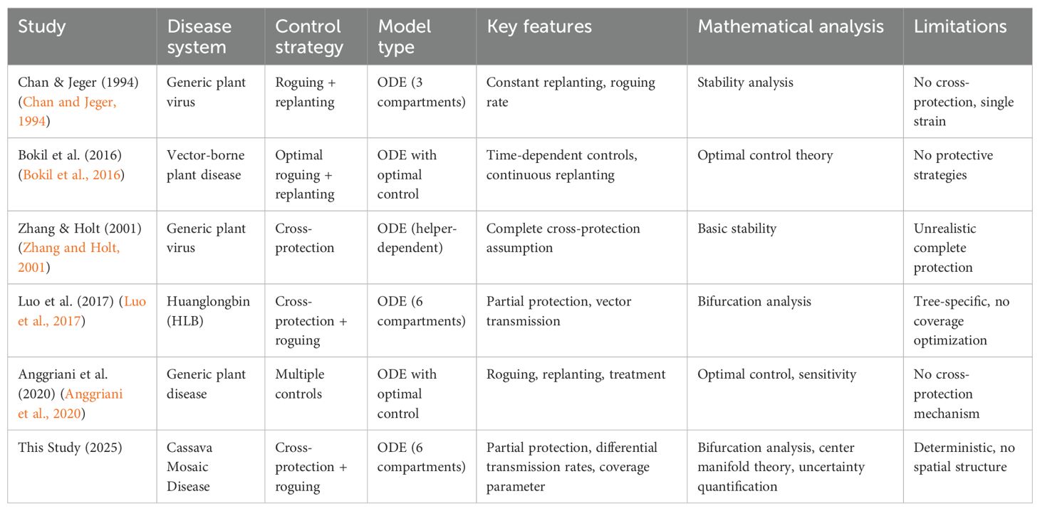
Table 1. Comparison of mathematical models for plant disease control strategies.

1.4 Mathematical contributions and novel features

This study addresses the theoretical gap by developing the first comprehensive mathematical framework for analyzing cross-protection in vector-borne plant diseases. Our key contributions: We (i) derive an explicit basic reproduction number R₀ that decomposes into plant–vector infection “cycles” (unprotected and cross-protected), clarifying how protection scales transmission; (ii) prove positivity and boundedness of the biologically feasible region and characterize equilibria; (iii) obtain local/global stability of the disease-free equilibrium with the sharp threshold R₀ = 1; (iv) provide an analytic criterion for backward bifurcation by deriving a quadratic condition in the protection parameter α, with parameter regime visualization to delineate forward vs. backward transitions; and (v) quantify parameter influence on R₀ and endemic burden using a reproducible uncertainty-quantification pipeline (LHS + PRCC). Together, these results yield management-relevant thresholds (minimum protection coverage and roguing intensity) while keeping the model minimal enough for transparent analysis and robust computation.

Our approach introduces several novel mathematical features.

1.4.1 Methodological innovations

● Differential transmission modeling: Incorporation of distinct transmission rates (${\beta }_1\ne {\beta }_2$, ${\beta }_3\ne {\beta }_4$) for protected vs. unprotected plants, capturing partial protection mechanisms

● Bifurcation analysis: Application of center manifold theory to identify conditions for backward bifurcation, revealing scenarios where R₀ < 1 does not guarantee disease elimination

● Implementation effectiveness quantification: Systematic analysis of the relationship between protection effectiveness and coverage requirements

1.4.2 Theoretical insights

● Identification of critical effectiveness thresholds where cross-protection transitions from supplementary to primary control strategy

● Demonstration of hysteresis effects in disease management under specific parameter regimes

● Quantification of trade-offs between implementation quality and coverage expansion

1.4.3 Practical applications

● Clear benchmarks for cross-protection research and development priorities

● Quantitative guidance for resource allocation in disease management programs

● Framework extensible to other vector-borne plant disease systems

Table 2 provides a summary of innovations.

Table 2

Table 2. Novel mathematical features of the current cross-protection framework.

These innovations collectively enable realistic assessment of cross-protection viability under field conditions while revealing complex dynamical phenomena. Partial protection is represented directly by differential transmission rates (${\beta }_2<{\beta }_1$, ${\beta }_4<{\beta }_3$), consistent with field evidence (e.g., ${\beta }_2\approx 0.5{\beta }_1, {\beta }_4\approx 0.5{\beta }_3$ formulation preserves closed-form analysis (e.g., $R_0$) and enables effectiveness optimization by reading off $R_0=1$ threshold contours for $(\alpha ,\sigma )$ at empirically grounded $({\beta }_2,{\beta }_4)$.

1.5 Paper organization and scope

The remainder of this paper develops our theoretical framework through rigorous mathematical analysis combined with uncertainty quantification to address implementation realities. Section 2 presents the model formulation and basic analysis, establishing equilibrium conditions and stability properties, including formal proofs of positivity, boundedness, and global stability of the disease-free equilibrium. Section 3 conducts comprehensive bifurcation analysis using center manifold theory to identify conditions for complex dynamics and backward bifurcation. Section 4 employs uncertainty and sensitivity analysis to explore parameter spaces relevant to practical implementation, quantifying the relative influence of model parameters on disease transmission potential. Section 5 provides numerical validation of theoretical predictions across different implementation scenarios, demonstrating the impact of cross-protection effectiveness on disease control outcomes. Section 6 discusses practical implications for CMD management, model limitations, and potential extensions to other vector-borne crop diseases. Section 7 concludes with a synthesis of key findings and their significance for disease management strategies.

Our analysis reveals that cross-protection effectiveness (rather than coverage expansion) represents the critical factor determining strategy viability, with implications extending beyond CMD to broader questions of protective interference in biological systems.

2 The basic model and its analysis

2.1 Model formulation

We develop a compartmental model that captures the dynamics of both plant and vector populations in the presence of cross-protection. The model structure reflects the biological reality that cross-protection provides partial, rather than complete, protection against virulent strains.

For the plant population, we define four compartments: X represents susceptible plants, Y denotes cross-protected and susceptible plants, Z represents infected but not cross-protected plants, and U denotes infected and cross-protected plants. The vector population is simplified to two compartments: S (susceptible vectors) and I (infected vectors). Our model extends classical plant disease frameworks (Chan and Jeger, 1994) by incorporating two key features: differential transmission rates for cross-protected plants (${\beta }_2<{\beta }_1$ for plant infection, ${\beta }_4<{\beta }_3$ for vector infection) and partial protection rather than complete immunity, reflecting field observations (Owor et al., 2004).

2.1.1 Biological interpretation of compartments

X: Susceptible plants (unprotected). Healthy plants with no cross-protective status; fully susceptible to infection from infectious vectors at rate β₁.

Y: Susceptible plants (cross-protected). Healthy plants that have cross-protection (e.g., prior mild exposure or induced protection); experience reduced transmission compared to X (infection from vectors at rate β₂ < β₁).

Z: Infected plants (no cross-protection). Actively infectious plants without cross-protection; transmit to vectors at rate β₃ and are subject to roguing at rate σ as well as natural/harvest losses.

U: Infected plants (cross-protected). Infectious plants that carry cross-protection; transmit to vectors at the reduced rate β₄ < β₃ and are also subject to roguing and other losses.

S: Susceptible vectors. Vectors (e.g., whiteflies) that have not yet acquired the pathogen; become infectious after feeding on Z or U.

I: Infectious vectors. Vectors carrying the pathogen; transmit to plants on subsequent feeds (to X at β₁, to Y at β₂) and experience natural and insecticide-induced mortality (rates µ and γ).

Let $N=X+Y+Z+U$ denote the total plant population, $V=S+I$ represent the total vector population, and K denote the carrying capacity of plants in the field. The model dynamics are governed by the following system of ordinary differential equations

$\begin{array}{ll}\frac{dX}{dt}={\alpha }_1(K-N)-\alpha X-(\delta +\omega )X-{\beta }_{1}XI& (1)\end{array}$

$\begin{array}{ll}\frac{dY}{dt}=\alpha X-(\delta +\omega )Y-{\beta }_{2}YI& (2)\end{array}$

$\begin{array}{ll}\frac{dZ}{dt}={\beta }_{1}XI-(\delta +\sigma +\omega )Z& (3)\end{array}$

$\begin{array}{ll}\frac{dU}{dt}={\beta }_{2}YI-(\delta +\sigma +\omega )U& (4)\end{array}$

$\begin{array}{ll}\frac{dS}{dt}=\text{Λ}-{\beta }_{3}SZ-{\beta }_{4}SU-(\mu +\gamma )S& (5)\end{array}$

$\begin{array}{ll}\frac{dI}{dt}={\beta }_{3}SZ+{\beta }_{4}SU-(\mu +\gamma )I& (6)\end{array}$

The biological interpretation and parameter definitions are detailed in Tables 3, 4. A schematic representation of the model structure is shown in Figure 1. Key model assumptions include homogeneous mixing within the field, constant cross-protection effectiveness over time, no co-infection dynamics (plants are either protected or infected with virulent strain), and faster timescales of vector population dynamics than plant dynamics. Unlike previous plant disease models that assume complete cross-protection (Zhang and Holt, 2001), our framework incorporates partial protection through differential transmission rates, enabling realistic analysis of implementation effectiveness.

Table 3

Table 3. Nomenclature (state variables).

Table 4

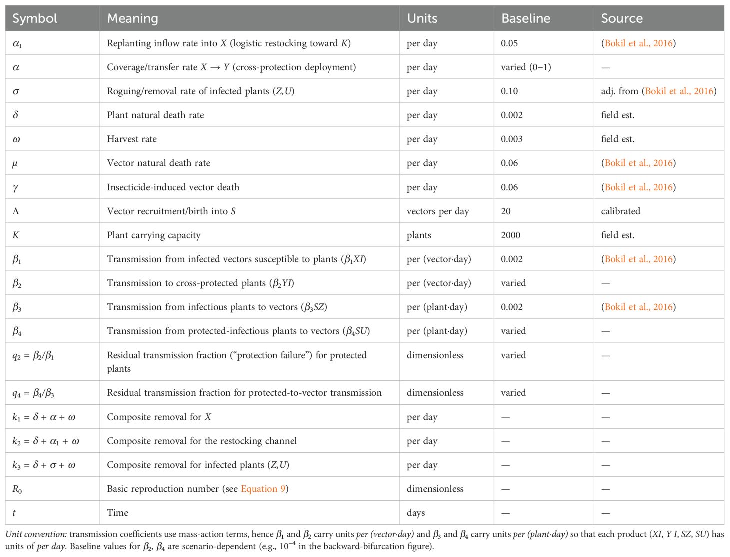
Table 4. Nomenclature (parameters and derived quantities). Baseline values are those used in simulations unless noted.

Figure 1

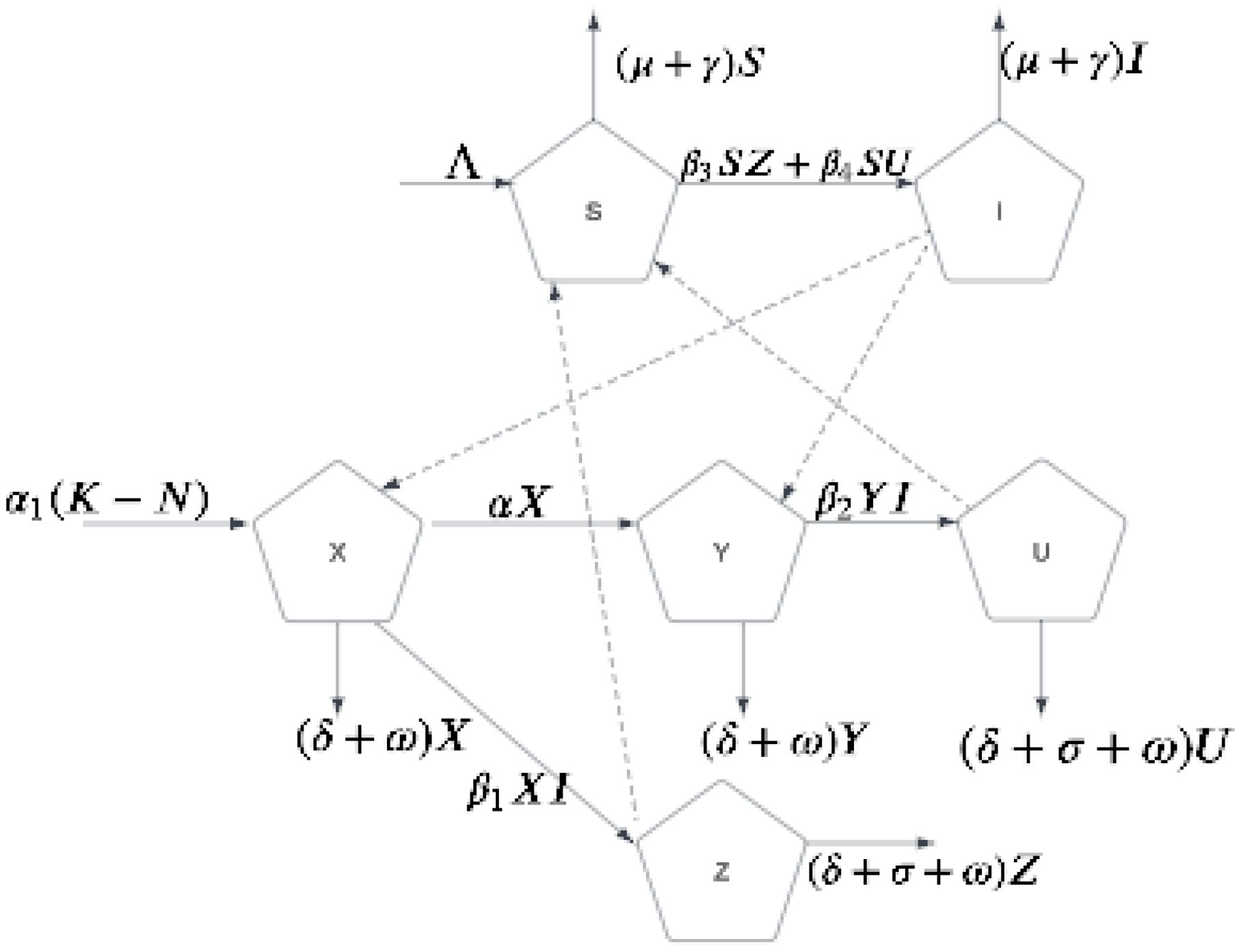
Figure 1. Compartmental model for CMD transmission with cross-protection. Plant compartments: X (susceptible), Y (cross-protected), Z (infected, non-cross-protected), U (infected, cross-protected). Vector compartments: S (susceptible), I (infected). Parameter effectiveness (β₂, β₄) determines whether cross-protection provides modest supplementary benefits or becomes a primary control strategy. While illustrated here for CMD, this model structure applies to any vector-borne plant disease system exhibiting partial cross-protection.

Before giving the main result, we present the following lemma.

Lemma 2.1. Let all parameters in system Equations 1–6 be positive and let the initial conditions satisfy

$X(0), Y(0), Z(0), U(0), S(0), I(0) \ge 0$

Then a solution of the system X(t), Y (t), Z(t), U(t), S(t), I(t) ≥ 0 for all t and the region is positively invariant for system (1)–(6).

$\text{Ω}=\left\{(X,Y,Z,U,S,I)\in {ℝ}_{+}^6: 0\le X+Y+Z+U\le K, 0\le S+I\le \frac{\Lambda }{\mu +\gamma }\right\}$

Proof. Nonnegativity follows from the quasi-positivity of the system: When any state variable reaches zero, its time derivative of (1)-(6) is non-negative, ensuring trajectories cannot exit the nonnegative orthant.

Let N = X + Y + Z + U and V = S + I. Then

$$\frac{dN}{dt}={\alpha }_1(K-N)-(\delta +\omega )N-\sigma (Z+U)\le {\alpha }_1(K-N), \frac{dV}{dt}=\text{Λ}-(\mu +\gamma )\mathit{V.}$$

Hence N(t) ≤ K and V(t) ≤ Λ/(µ + γ) for all t ≥ 0, showing positive invariance of Ω.

A related proof for a spatially extended CMD system confirming this behavior is provided in (Oh, 2025).

2.2 Parameter interpretation and uncertainty

A critical aspect of this model is the relationship between cross-protection effectiveness and the transmission parameters β₂ and β₄. Field studies by Owor et al (Owor et al., 2004). suggest that cross-protected plants exhibit infection rates approximately 50% of unprotected plants, implying β₂ ≈ 0.5β₁ and β₄ ≈ 0.5β₃. However, this empirical ratio represents current implementation methods and may not reflect the theoretical potential of optimized cross-protection strategies.

For generalization, we introduce a dimensionless parameter q_i ∈ (0, 1) for i = 1, 2 representing the residual transmission fraction

$${\beta }_2=q_1{\beta }_1, {\beta }_4=q_2{\beta }_{3.}$$

Smaller q_i indicates stronger cross-protection (e.g., q_i = 0.5 means protected transmission is 50% of the unprotected rate, corresponding to 50% protection efficacy).

The cross-protection parameter α represents the proportion of newly planted susceptible plants that receive cross-protection treatment. This parameter is central to our bifurcation analysis, as it determines the balance between protected and unprotected plant populations. Given these parameter relationships, we next examine how uncertainty in their estimation affects model predictions.

Effectiveness optimization readout. We visualize the trade-off between coverage and roguing by plotting R₀(α, σ; β₂, β₄) = 1 contours at representative transmission pairs inferred from the literature, which provides a practical readout of “how much coverage or roguing is enough” for given effectiveness levels, see Figure 2.

Figure 2

Figure 2. Threshold countours of R₀(α, σ; β₂, β₄) = 1 with baseline parameters from Table 4. Curves show the trade-off between coverage α and roguing σ under representative protected transmission rates (β₂, β₄). Points below a contour yield R₀ < 1.

2.3 Equilibrium analysis

2.3.1 Disease-free equilibrium

Setting the infected compartments Z = U = I = 0, we obtain the disease-free equilibrium

$$E_0=\left(\frac{{\alpha }_{1}K(\delta +\omega )}{k_1{k}_2},\frac{\alpha {\alpha }_{1}K}{k_1{k}_2},0,0,\frac{\text{Λ}}{\mu +\gamma },0\right)$$

where k₁ = δ + α + ω and $k_2=\delta +{\alpha }_1+\omega .$

2.3.2 Basic reproduction number

To assess the stability of the disease-free equilibrium, we calculate the basic reproduction number R₀ using the next generation operator method (Diekmann and Heesterbeek, 2000). We focus on the infected classes E = [Z, U, I] and define

$\begin{array}{ll}ℱ=\left(\begin{array}{c}{\beta }_1{X}_{0}I\\ {\beta }_2{Y}_{0}I\\ {\beta }_3{S}_{0}Z+{\beta }_4{S}_{0}U\end{array}\right),\mathcal{V}=\left(\begin{array}{c}(\delta +\sigma +\omega )Z\\ (\delta +\sigma +\omega )U\\ (\mu +\gamma )I\end{array}\right)& (7)\end{array}$

The corresponding Jacobian matrices are

$\begin{array}{ll}F=\left(\begin{array}{ccc}0& 0& {\beta }_1{X}_0\\ 0& 0& {\beta }_2{Y}_0\\ {\beta }_3{S}_0& {\beta }_4{S}_0& 0\end{array}\right),V=\left(\begin{array}{ccc}\delta +\sigma +\omega & 0& 0\\ 0& \delta +\sigma +\omega & 0\\ 0& 0& \mu +\gamma \end{array}\right)& (8)\end{array}$

The basic reproduction number R₀ is given by the spectral radius of FV ⁻¹

$$R_0:=\rho (F{V}^{-1})=\sqrt{\frac{{\beta }_3{\beta }_1{S}_0{X}_0+{\beta }_2{\beta }_4{S}_0{Y}_0}{(\mu +\gamma )(\delta +\sigma +\omega )}}.$$

Substituting the disease-free equilibrium values

$\begin{array}{ll}{R}_0=\sqrt{\frac{{\beta }_3{\beta }_1\text{Λ}{\alpha }_{1}K(\delta +\omega )+{\beta }_2{\beta }_4\text{Λ}\alpha {\alpha }_{1}K}{{(\mu +\gamma )}^2{k}_1{k}_2{k}_3}}& (9)\end{array}$

where k₃ = δ + σ + ω. Note that the basic reproduction number R₀ has additive contributions from unprotected transmission cycle $\frac{{\beta }_3{\beta }_1{\text{Λα}}_{1}K(\delta +\omega )}{{(\mu +\gamma )}^2{k}_1{k}_2{k}_3}$ and cross-protected transmission cycle $\frac{{\beta }_2{\beta }_4{\text{Λαα}}_{1}K}{{(\mu +\gamma )}^2{k}_1{k}_2{k}_3}$. The relative magnitude of these terms determines whether cross-protection investment (increasing α) effectively reduces disease transmission.

2.3.3 Stability of disease-free equilibrium

Theorem 2.2. The disease-free equilibrium E₀ is locally asymptotically stable when R₀ < 1 and unstable when R₀ > 1.

Proof. The stability is determined by the eigenvalues of the Jacobian matrix at E₀. Five eigenvalues are explicitly negative, while the sixth eigenvalue changes sign at R₀ = 1, confirming the stability condition.

Lemma 2.3. If R₀ < 1, then the disease-free equilibrium E₀ is globally asymptotically stable in Ω.

Proof. Let the infected subsystem be written as $\dot{E}$ = $ℱ$(E) − $\mathcal{V}$(E), where $ℱ$ and $\mathcal{V}$ denote the new-infection and transition terms as in Equation 7, respectively, and F = D_E $ℱ$(E₀), $\mathcal{V}$ = D_E $\mathcal{V}$(E₀) in Equation 8. By Lemma 2.1, all trajectories remain in the positively invariant region Ω. Following Theorem 2.2 of Shuai and van den Driessche (2013), consider the linear Lyapunov function ℒ(E) = w^⊤V ⁻¹E, where w > 0 is the left Perron eigenvector of FV ⁻¹ associated with R₀. Then $\dot{ℒ}$ ≤ (R₀ − 1) w^⊤E, which is strictly negative for E ≠ 0 when R₀ < 1. By LaSalle’s invariance principle, all trajectories converge to E₀, proving global stability.

2.4 Endemic equilibrium

For the endemic equilibrium where infection persists (Z*, U*, I* > 0), we solve the system at steady state. The analysis reveals that endemic equilibria exist when R₀ > 1, but the possibility of backward bifurcation means that endemic states may also exist for certain parameter ranges when R₀ < 1.

The endemic equilibrium components can be expressed in terms of I* as

$$S^{*}=\frac{\text{Λ}}{\mu +\gamma }-I^{*}$$

$$Y^{*}=\frac{\alpha {(\mu +\gamma )}^2(\delta +\sigma +\omega )}{{\beta }_1{\beta }_3(\text{Λ}-(\mu +\gamma )I^{*})(\delta +\omega +{\beta }_2{I}^{*})+\alpha {\beta }_2{\beta }_4(\text{Λ}-(\mu +\gamma )I^{*})}$$

$$X^{*}=\frac{{(\mu +\gamma )}^2(\delta +\sigma +\omega )(\delta +\omega +{\beta }_2{I}^{*})}{{\beta }_1{\beta }_3(\text{Λ}-(\mu +\gamma )I^{*})(\delta +\omega +{\beta }_2{I}^{*})+\alpha {\beta }_2{\beta }_4(\text{Λ}-(\mu +\gamma )I^{*})}$$

The value of I* is determined by solving a quadratic equation, leading to the possibility of multiple endemic equilibria under certain parameter conditions. Having established the model structure and basic equilibrium properties, we now investigate the conditions under which complex bifurcation phenomena emerge.

3 Bifurcation analysis

3.1 Endemic equilibrium existence

To understand the long-term behavior of the system when disease persists, we analyze the endemic equilibrium where Z*, U*, I* > 0. Setting system (1)-(6) to zero and solving for the equilibrium values in terms of I*, we obtain

$\begin{array}{ll}{S}^{*}=\frac{\text{Λ}}{\mu +\gamma }-I^{*}& (10)\end{array}$

$\begin{array}{ll}{Y}^{*}=\frac{\alpha {(\mu +\gamma )}^2(\delta +\sigma +\omega )}{{\beta }_1{\beta }_3(\text{Λ}-(\mu +\gamma )I^{*})(\delta +\omega +{\beta }_2{I}^{*})+\alpha {\beta }_2{\beta }_4(\text{Λ}-(\mu +\gamma )I^{*})}& (11)\end{array}$

$\begin{array}{ll}{X}^{*}=\frac{{(\mu +\gamma )}^2(\delta +\sigma +\omega )(\delta +\omega +{\beta }_2{I}^{*})}{{\beta }_1{\beta }_3(\text{Λ}-(\mu +\gamma )I^{*})(\delta +\omega +{\beta }_2{I}^{*})+\alpha {\beta }_2{\beta }_4(\text{Λ}-(\mu +\gamma )I^{*})}& (12)\end{array}$

$\begin{array}{ll}{Z}^{*}=\frac{{(\mu +\gamma )}^2{\beta }_1{I}^{*}(\delta +\omega +{\beta }_2{I}^{*})}{{\beta }_1{\beta }_3(\text{Λ}-(\mu +\gamma )I^{*})(\delta +\omega +{\beta }_2{I}^{*})+\alpha {\beta }_2{\beta }_4(\text{Λ}-(\mu +\gamma )I^{*})}& (13)\end{array}$

$\begin{array}{ll}{U}^{*}=\frac{\alpha {(\mu +\gamma )}^2{\beta }_2{I}^{*}}{{\beta }_1{\beta }_3(\text{Λ}-(\mu +\gamma )I^{*})(\delta +\omega +{\beta }_2{I}^{*})+\alpha {\beta }_2{\beta }_4(\text{Λ}-(\mu +\gamma )I^{*})}& (14)\end{array}$

Substituting Equations 10–14 into the equation for $\frac{dI}{dt}$ = 0, we obtain a quadratic equation in I*

$$h(I^{*})=a{I}^{*2}+b{I}^{*}+c=0$$

where the coefficients are

$$a={\alpha }_{1}K(\mu +\gamma ){\beta }_1{\beta }_2{\beta }_3+{(\mu +\gamma )}^2{\beta }_1{\beta }_2{k}_4$$

$$b={\alpha }_{1}K{\beta }_1{\beta }_3((\delta +\omega )(\mu +\gamma )-\text{Λ}{\beta }_2)+\alpha {\alpha }_{1}K(\mu +\gamma ){\beta }_2{\beta }_4+{(\mu +\gamma )}^2{\beta }_2{k}_3{k}_5+{(\mu +\gamma )}^2{\beta }_1(\delta +\omega )k_4+\alpha {\alpha }_1{(\mu +\gamma )}^2{\beta }_2$$

$$c={(\mu +\gamma )}^2{k}_1{k}_2{k}_3(1-R_0^2)$$

with k₄ = δ + σ + ω + α₁ and k₅ = δ + ω + α + α₁. Since all parameters are positive, we have a > 0. Using the quadratic formula with discriminant Δ = b² − 4ac, the roots are

$\begin{array}{ll}{I}_{1,2}^{*}=\frac{-b\pm \sqrt{\text{Δ}}}{2a}& (15)\end{array}$

The preceding analysis leads directly to the following theorem.

Theorem 3.1. The existence and number of positive endemic equilibria depend on R₀ in Equation 9 as follows

1. If R₀ > 1, then c < 0, implying Δ > 0 and exactly one positive root $I_2^{*}=\frac{-b+\sqrt{\text{Δ}}}{2a}$. The system has a unique endemic equilibrium E₂.

2. If R₀ = 1, then c = 0 and Δ = b². We obtain roots $I_1^{*}=0$ and $I_2^{*}=-\frac{b}{a}$. A unique positive endemic equilibrium E₂ exists if and only if b < 0.

3. If R₀ < 1, then c > 0, leading to two subcases

(a) If b > 0, no positive roots exist.

(b) If b < 0 and Δ > 0, two positive endemic equilibria E₁ and E₂ exist, indicating the possibility of backward bifurcation

The critical insight from case 3(b) is that the system can sustain endemic disease levels even when R₀ < 1, provided the cross-protection parameter α falls within a specific range. This backward bifurcation phenomenon has significant implications for disease control strategies.

The existence of multiple endemic equilibria when R₀ < 1 has profound implications for disease control:

1. High initial infection levels may prevent disease elimination even with R₀ < 1

2. Control efforts must achieve R₀ < R^c (sub-threshold value) to guarantee elimination

3. Gradual implementation may trap the system in high-endemic states.

3.2 Conditions for backward bifurcation

Backward bifurcation occurs when a stable endemic equilibrium coexists with the stable disease-free equilibrium for R₀ < 1. This phenomenon arises due to the complex interaction between cross-protection effectiveness and disease transmission dynamics.

From our analysis, backward bifurcation is possible when R₀ < 1 (below the classical epidemic threshold), b< 0 (ensuring positive endemic equilibria exist) and Δ > 0 (ensuring real roots).

The parameter α (proportion of plants receiving cross-protection) plays a crucial role in determining these conditions. There exists a critical range α^∗< α< α^∗∗ where backward bifurcation occurs, meaning that

1. Multiple stable states coexist: Both disease-free and endemic equilibria can be stable simultaneously.

2. Hysteresis effects: The final disease state may depend on the initial conditions and how parameters change over time.

3. Control thresholds are elevated: Reducing R₀ below 1 may not guarantee disease elimination.

Backward bifurcation occurs when the nonlinear feedback between cross-protection coverage and disease transmission creates alternative stable states. This happens when cross-protection is highly effective (small β₂, β₄), coverage is in an intermediate range, and the protective benefits outweigh the maintenance of infected populations. The incorporation of coverage-dependent partial protection creates the potential for complex bifurcation phenomena not observed in traditional plant disease models, necessitating rigorous dynamical systems analysis.

3.3 Center manifold analysis for backward bifurcation

Center manifold theory provides a powerful technique for understanding the behavior of dynamical systems near critical parameter values where stability changes occur. When the system reaches the bifurcation point (R₀ = 1), the linearized system has a zero eigenvalue, making standard linear stability analysis insufficient. The center manifold approach reduces the high-dimensional system to its essential dynamics on a lower-dimensional manifold where the critical behavior unfolds. By projecting the full six-dimensional dynamics onto this center manifold-essentially the “slow” direction along which the bifurcation occurs-we can determine whether the system exhibits forward bifurcation (where disease smoothly appears as R₀ crosses 1) or backward bifurcation (where multiple equilibria can coexist, creating the possibility of disease persistence even when R₀ < 1). The sign of specific coefficients in this reduced system reveals which type of bifurcation occurs.

To determine the precise conditions under which backward bifurcation occurs, we employ center manifold theory following the approach of Castillo-Chavez and Song (2004). Setting R₀ = 1 is equivalent to

$$d=\overline{d}:=\sqrt{\frac{{\beta }_3{\beta }_1\text{Λ}{\alpha }_{1}K(\delta +\omega )+{\beta }_2{\beta }_4\text{Λ}\alpha {\alpha }_{1}K}{k_1{k}_2{k}_3}}$$

where d = µ + γ serves as our bifurcation parameter. The disease-free equilibrium E₀ is locally stable when d < $\overline{d}$ and unstable when d > $\overline{d}$.

At the bifurcation point R₀ = 1, the Jacobian matrix J(E₀) has a simple zero eigenvalue which implies that the center manifold is one dimensional. We parametrize the center manifold by c(t). By Theorem 4.1 in (Castillo-Chavez and Song, 2004) we can determine the direction of bifurcation by computing two key quantities $\tilde{A}$ and $\tilde{B}$ in the first order differential equation of c(t) which comes from the invariance of the center manifold. We express $\tilde{A}$ and $\tilde{B}$ in terms of parameters below.

The right eigenvector corresponding to the zero eigenvalue is w = (w₁, w₂, w₃, w₄, w₅, w₆)^T, where each component can be expressed in terms of w₆

$$w_1=\frac{(\omega +\sigma ){\alpha }_1{\beta }_2{w}_6-{\beta }_1{X}_0(\delta +\omega )k_4{w}_6}{k_1{k}_2{k}_3}$$

$$w_2=\frac{-\alpha {\beta }_1{X}_0{k}_4{w}_6-{\beta }_2{Y}_0(\alpha {\alpha }_1+k_3{k}_5)w_6}{k_1{k}_2{k}_3}$$

$$w_3=\frac{{\beta }_1{X}_0{w}_6}{k_3}, w_4=\frac{{\beta }_2{Y}_0{w}_6}{k_3}$$

$$w_5=-w_6,w_6=w_6$$

The left eigenvector is v = (v₁, v₂, v₃, v₄, v₅, v₆)^T with

$$v_1=v_2=v_5=0$$

$$v_3=\frac{{\beta }_3{S}_0{v}_6}{k_3}, v_4=\frac{{\beta }_4{S}_0{v}_6}{k_3}, v_6=v_6$$

We choose v₆ and w₆ such that v · w = 1.

Following center manifold theory, the reduced dynamics on the center manifold are governed by

$$\frac{dc}{dt}=\frac{\tilde{A}}{2}{c}^2+\tilde{B}\varphi c$$

where $\varphi =d-\overline{d}$ is the bifurcation parameter and

$$\tilde{A}={\sum }^{ }{v}_k{w}_i{w}_j\frac{{\partial }^2{f}_k}{\partial x_i\partial x_j}(0,0)=-\frac{g(\alpha )}{k_3^2{k}_1{k}_2}{v}_6{w}_6^2$$

$$\tilde{B}=\sum v_k{w}_i\frac{{\partial }^2{f}_k}{\partial x_i\partial \varphi }(0,0)=w_6{v}_6>0$$

where

$\begin{array}{ll}g(\alpha )=A_1{\alpha }^2+A_2\alpha +A_3& (16)\end{array}$

with coefficients:

$$A_1={\beta }_4{\beta }_2^2\text{Λ}({\alpha }_1+k_3)+{\beta }_2{\beta }_4{k}_2{k}_3(\mu +\gamma )>0$$

$$A_2=-\text{Λ}{\alpha }_1{\beta }_1{\beta }_2{\beta }_3(\sigma +\omega )+\text{Λ}{\alpha }_1{\beta }_2^2{\beta }_4{k}_3+\text{Λ}{\beta }_1{\beta }_2{\beta }_4(\delta +\omega )k_4+\text{Λ}{\beta }_2^2{\beta }_4(\delta +\omega )k_3-k_2{k}_3(\mu +\gamma ){\beta }_1{\beta }_3(\delta +\omega )+k_2{k}_3(\mu +\gamma )(\delta +\omega ){\beta }_2{\beta }_4$$

$$A_3=\text{Λ}{\beta }_1^2{\beta }_3{(\delta +\omega )}^2{k}_4-k_2{k}_3(\mu +\gamma ){(\delta +\omega )}^2{\beta }_1{\beta }_3$$

We next state the precise condition under which a backward (subcritical) bifurcation in the coverage parameter α can occur.

Theorem 3.2. System (1)-(6) undergoes a backward bifurcation at R₀ = 1 if and only if Δ′ > 0, A₂ < 0, and α^∗< α < α^∗∗, where:

$${\alpha }^{\ast }=\frac{-A_2-\sqrt{{\Delta }^{\prime }}}{2A_1},{\alpha }^{\ast \ast }=\frac{-A_2+\sqrt{{\Delta }^{\prime }}}{2A_1}$$

and ${\Delta }^{\prime }=A_2^2-4A_1{A}_3$ is the discriminant of g(α) in Equation 16.

Proof. The result follows from Theorem 4.1 in (Castillo-Chavez and Song, 2004). Backward bifurcation occurs when $\tilde{A}$ > 0 and $\tilde{B}$ > 0, which is equivalent to g(α) < 0. Since A₁ > 0, the condition g(α) < 0 is satisfied when α lies between the two positive roots of g(α) = 0, provided they exist (i.e., Δ′ > 0 and A₂ < 0).

Remark 3.3. A backward (subcritical) bifurcation in α is possible iff

$$\Delta \prime >0, {\alpha }^{\ast }, {\alpha }^{\ast \ast }\in (0,1), and \alpha \in ({\alpha }^{\ast },{\alpha }^{\ast \ast })$$

in addition to R₀ < 1. The dependence of Δ′ on (β₂, β₄, σ) is determined by the explicit coefficient formulas A₁, A₂, A₃ given above; hence, the quadratic criterion (21) defines analytically the parameter ranges for backward bifurcation, consistent with the bifurcation curves shown in Figures 3, 4.

Figure 3

Figure 3. Backward (subcritical) bifurcation. Endemic prevalence (Z+U)/K versus coverage α. Solid blue: endemic stable; dashed orange: endemic unstable. The disease-free equilibrium (DFE) is plotted at 0 (green solid when R₀ < 1, red dashed when R₀ > 1). The fold marks the boundaries of a bistable interval where the DFE and an endemic equilibrium coexist even with R₀ < 1, demonstrating hysteresis. (a) β₂, β₄ = 0.0001, σ = 0.1 (b) β₂, β₄ = 0.0001, σ = 0.12.

Figure 4

Figure 4. Bifurcation diagrams showing endemic equilibrium infectious populations versus cross-protection coverage α for (a) Scenario A: Forward bifurcation only, (b) Scenario B: Transition zone with a hint of stable endemic equilibrium (backward bifurcation), (c) Scenario C: Clear backward bifurcation occurs for α ∈ (0.63,0.7) when σ = 0.1. Solid lines represent stable equilibria; dashed lines represent unstable equilibria.

Remark 3.4. In the backward bifurcation regime, there exists a sub-threshold value $R_0^c<1$ such that for $R_0^c<R_0<1$, the stable disease-free equilibrium coexists with a stable endemic equilibrium. This implies that reducing $R_0$ below 1 may not guarantee disease elimination, and control strategies must aim for $R_0<R_0^c$.

Remark 3.5. The analytical condition for backward bifurcation obtained in Theorem 3.2 is illustrated numerically in Figures 3, 4. Figure 3 shows that, for fixed β₂ and β₄, increasing the roguing rate σ shifts the backward-bifurcation window toward smaller α values, indicating that stronger roguing reduces the coverage threshold required for disease elimination. In contrast, Figure 4 compares bifurcation diagrams for different (β₂, β₄) with the same σ. Reducing β₂ and β₄ is the correct lever to push R₀ < 1, but we find that reducing β₂ and β₄, equivalently reducing the value of the residual transmission fraction q₁,₂, produces a wider backward bifurcation window in α ∈ (0,1). This has profound implications: Strong per plant cross-protection makes control harder. Hence, cross-protection should be optimized—not merely maximized—to avoid regimes where R₀ < 1 does not ensure disease elimination. See Section 5.3.1 for details.

3.4 Implications for cross-protection strategy

The bifurcation analysis reveals that the effectiveness of cross-protection as a control strategy is highly dependent on implementation quality

● Under empirically observed parameters (β₂ ≈ 0.5β₁), forward bifurcation typically occurs, and cross-protection provides modest benefits.

● Under optimized cross-protection scenarios (β₂ ≪ β₁), backward bifurcation becomes possible in certain parameter ranges, creating complex dynamics where disease persistence depends on initial conditions.

● The backward bifurcation phenomenon suggests that even highly effective cross-protection may not guarantee disease elimination if implementation coverage, α, falls within specific ranges.

This analysis motivates our subsequent uncertainty quantification to identify the parameter combinations under which cross-protection transitions from a supplementary to a primary control strategy. The bifurcation analysis reveals theoretical possibilities, but practical implementation requires understanding parameter uncertainty impacts.

4 Uncertainty and sensitivity analysis

Having established the theoretical framework and identified conditions for complex dynamical phenomena including backward bifurcation, we now apply this general model to evaluate cross-protection as a control strategy for Cassava Mosaic Disease. CMD serves as an exemplary case study due to its economic importance, documented cross-protection potential from field trials, and the availability of empirical data on protective effectiveness. This application demonstrates how the theoretical insights from Sections 2–3 translate into practical guidance for disease management. Through comprehensive uncertainty and sensitivity analyses, we explore the parameter space relevant to CMD while identifying which factors most critically determine the success of cross-protection strategies. The methodology developed here illustrates how the general framework can be applied to specific vector-borne plant disease systems to evaluate the viability of protective interference as a control mechanism.

4.1 Parameter uncertainty quantification

Given the limited empirical data (Owor et al., 2004) on cross-protection effectiveness, we conduct a comprehensive uncertainty and sensitivity analysis to explore the parameter space where cross-protection could provide meaningful disease control. This analysis addresses two critical questions: (1) What improvements in implementation are required for cross-protection to become viable? (2) Which parameters most strongly influence system outcomes?

Based on field studies and literature review, we assess parameter uncertainty by drawing N = 10,000 Latin Hypercube samples (SciPy QMC; fallback to simple LHS if QMC is unavailable; seed = 12345) over predefined ranges with the baselines from Table 4. The parameters are categorized into three groups based on confidence in their estimation.

4.1.1 Well-characterized parameters (narrow uncertainty ranges)

● Plant natural death rate: δ ∼ Uniform[0.0015,0.0025] (per day)

● Vector natural death rate: µ ∼ Uniform[0.05,0.07] (per day)

● Harvesting rate: ω ∼ Uniform[0.002,0.004] (per day)

● Replanting rate: α₁ ∼ Uniform[0.04,0.06] (per day)

4.1.2 Moderately uncertain parameters

• Roguing rate: σ ∼ Uniform[0.05,0.15] (per day)

• Insecticide mortality: γ ∼ Uniform[0.04,0.08] (per day)

• Vector reproduction: Λ ∼ Uniform [15,25] (per day)

• Non-cross-protected transmission: β₁ ∼ Uniform[0.0015,0.0025], β₃ ∼ Uniform[0.0015,0.0025] (per day)

4.1.3 Highly uncertain parameters (wide ranges reflecting implementation variability)

● Cross-protection coverage: α ∼ Uniform[0,1]

● Cross-protected transmission rates: β₂, β₄ ∼ Uniform[0.0001,0.001] (per day)

The range for β₂ and β₄ spans from highly effective cross-protection (0.0001, representing 20-fold reduction) to empirically observed values (0.001, representing 2-fold reduction relative to β₁ and β₃).

4.2 Global sensitivity analysis

Partial Rank Correlation Coefficients (PRCC) were computed between each sampled parameter and R₀ to quantify monotonic influences on transmission potential. Figure 5 displays the PRCC results; parameters with |PRCC| close to 1 exert the strongest influence. Table 5 lists the five most influential parameters and their biological interpretations with p-value threshold for statistical significance.

Figure 5

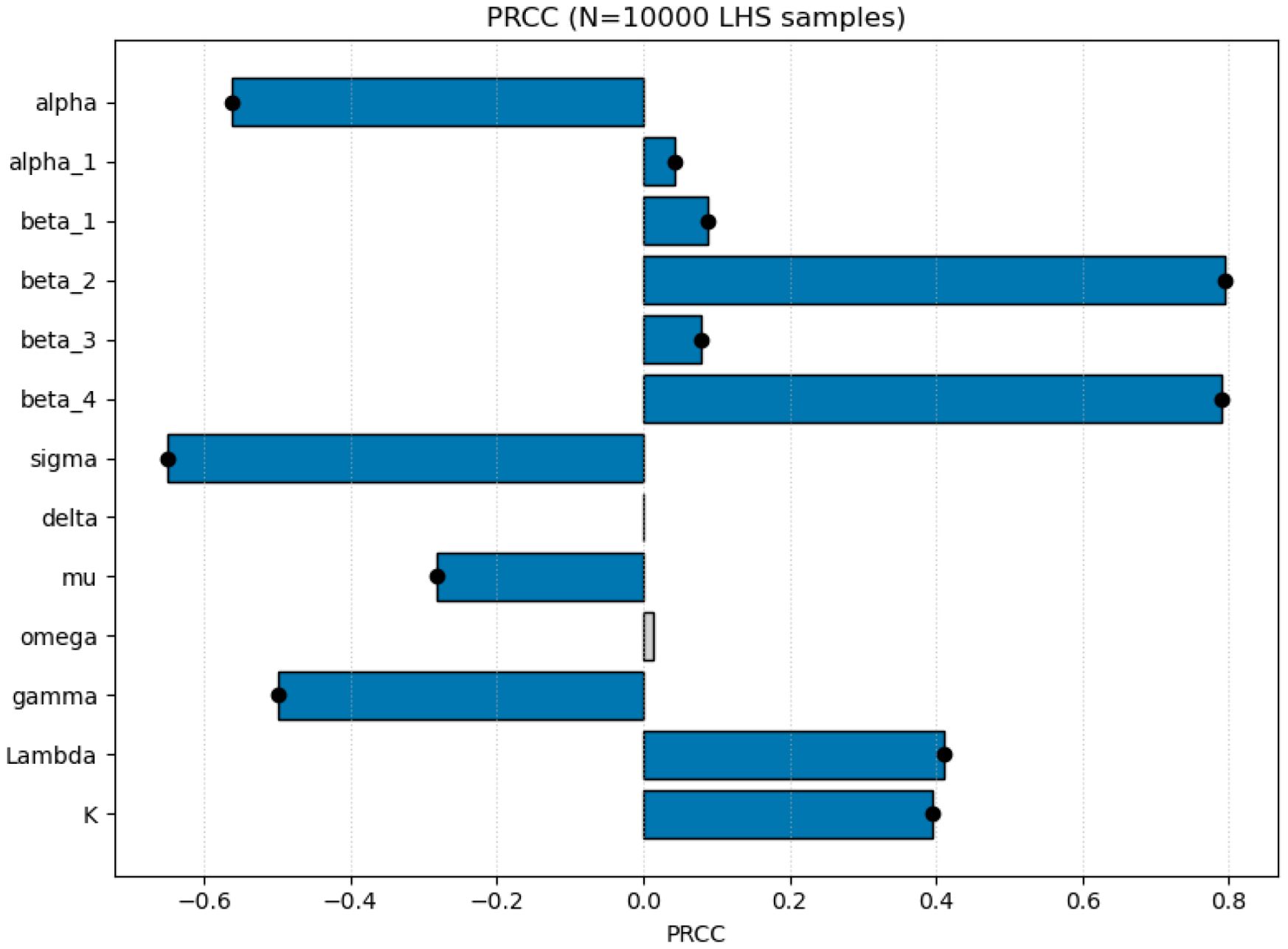
Figure 5. Partial rank correlation coefficients (PRCC) between model parameters and R₀. Black dots mark parameters with p< 0.05. Positive values indicate parameters that increase transmission potential; negative values indicate parameters that suppress R₀.

Table 5

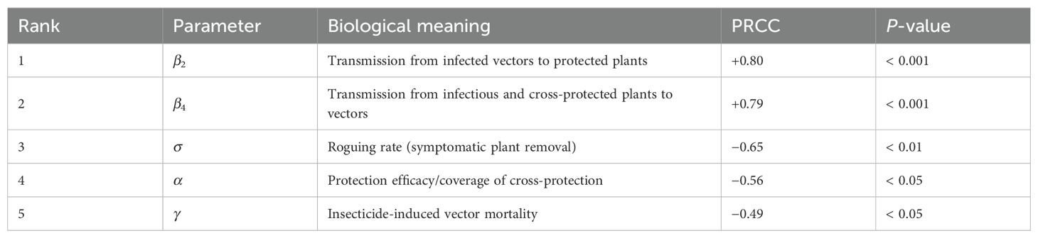
Table 5. Top five parameters ranked by absolute PRCC with respect to R₀. Signs indicate direction of association.

Interpretation. The PRCC ranking shows that the two transmission parameters (β₂ and β₄) dominate the variation in R₀, implying that CMD invasion is most sensitive to higher transmission rates (indicating less effective protection) substantially increase R₀, while the negative correlation for cross-protection coverage (α) shows that expanded implementation reduces disease transmission potential. The negative coefficients for the roguing rate (σ) and vector mortality rate (γ) confirm their roles in suppressing disease spread, although their quantitative effects are weaker than those of the transmission parameters.

Overall, the sensitivity results emphasize that while improving cross-protection and timely roguing remain essential, managing the effective transmission process—through vector control, virus-resistant varieties, or both—offers the most direct route to reducing R₀. These quantitative insights guide the management discussion presented in Section 6.

5 Numerical simulations

5.1 Parameter selection and scenarios

Based on the uncertainty analysis in Section 4, we design numerical experiments to illustrate the theoretical findings under different cross-protection implementation scenarios. We consider three distinct scenarios that span the range from current empirical evidence to optimized theoretical implementations. The baseline parameters, derived from literature and field studies, are presented in Table 4.

5.1.1 Cross-protection scenarios

We examine three scenarios representing different levels of cross-protection implementation success.

5.1.1.1 Scenario A: current field performance

• β₂ = 0.001, β₄ = 0.001 (2-fold protection)

• Based on empirical data from Owor et al. (Owor et al., 2004)

• Represents current implementation limitations

• R₀ ≈ 9.81 with no cross-protection (α = 0)

5.1.1.2 Scenario B: enhanced implementation

● β₂ = 0.0002, β₄ = 0.0002 (10-fold protection)

● Represents improved strain selection and deployment methods

● Intermediate effectiveness scenario

● Potential target for optimized field implementation

5.1.1.3 Scenario C: optimized cross-protection

• β₂ = 0.0001, β₄ = 0.0001 (20-fold protection)

• Represents theoretical potential with ideal implementation

• Used to explore mathematical phenomena (backward bifurcation)

• Upper bound for cross-protection effectiveness

5.2 Disease dynamics and equilibrium behavior

5.2.1 Time series analysis

Figure 6 demonstrates the temporal dynamics under Scenario C (optimized cross-protection) with α = 0.4, showing rapid decrease of susceptible plants and increase of cross-protected plants. Trajectories approach a low endemic equilibrium illustrating persistence near threshold.

Figure 6

Figure 6. Time series plot for all compartments (α was kept constant at 0.4).

To examine the impact of cross-protection coverage more systematically, Figure 7 shows how infectious compartments respond to different coverage levels under optimized implementation.

Figure 7

Figure 7. Disease dynamics under varying cross-protection coverage (α ∈{0,0.4,0.8}) showing infectious compartments Z (non-cross-protected) and U (cross-protected) under Scenario C parameters (20-fold protection). Higher coverage substantially reduces total infectious load, demonstrating the theoretical potential of optimized implementation.

The simulations reveal distinct behavioral patterns across coverage levels. Under Scenario C conditions, increasing cross-protection coverage from α = 0 to α = 0.8 produces dramatic reductions in both infectious compartments, with total infectious load decreasing by over 99%. The non-cross-protected infectious population (Z) shows the steepest decline, while the cross-protected infectious population (U) initially increases with coverage but remains at manageable levels.

The theoretical potential of optimized cross-protection implementation, where coverage expansion produces substantial disease control benefits, is demonstrated. However, these results represent upper-bound scenarios that require significant improvements over current field performance (Scenario A), where similar coverage changes would produce much more modest effects.

5.2.1.1 Scenario A (current performance)

• Only modest reduction in disease prevalence, even with high coverage levels (α = 0.8)

• Z* (non-protected infectious) decreases linearly with α

• U* (protected infectious) increases initially then plateaus

• Total infectious load (Z^*+ U^*) shows minimal reduction

5.2.1.2 Scenario B (enhanced implementation)

• Significant disease reduction achievable with moderate coverage

• Nonlinear relationship between coverage and disease burden

• Cross-over point around α = 0.4 where benefits accelerate

• Total infectious load shows meaningful reduction (> 50%) at medium coverage

5.2.1.3 Scenario C (optimized cross-protection)

• Dramatic disease reduction possible with relatively low coverage

• Threshold effects visible around α ≈ 0.5

• Near-elimination achievable with α > 0.7 (outside the backward-bifurcation window, see Figure 4C)

• Demonstrates theoretical potential of optimized cross-protection

5.3 Bifurcation analysis and multiple equilibria

5.3.1 Bifurcation diagrams

Figure 4 presents bifurcation diagrams showing endemic equilibrium values as functions of the cross-protection coverage parameter α. Detailed numerical bifurcation analysis confirms theoretical predictions in Section 3.3. These results show that stronger cross-protection (smaller β₂, β₄) enhances bistability, whereas high transmission suppresses it.

Scenario A: Forward transcritical bifurcation occurs at R₀ = 1 for all values of α ∈ [0,1]. No backward bifurcation observed, consistent with limited cross-protection effectiveness.

Scenario B: Predominantly forward bifurcation with hints of backward bifurcation in narrow parameter ranges (α ≈ 1). Represents transition zone where implementation improvements could access complex dynamics.

Scenario C: Clear backward bifurcation occurs, demonstrating multiple stable equilibria coexistence. Increasing the roguing rate σ shifts the backward-bifurcation range toward smaller α values—from approximately (0.625,0.70) at σ = 0.10 to (0.50,0.57) at σ = 0.12—showing that more intensive roguing enables control at lower coverage (see Figure 3). This confirms theoretical predictions and shows practical importance of initial conditions in disease management.

In Figure 8, the graph demonstrates how cross-protection effectiveness fundamentally alters the relationship between coverage and disease transmission potential. Under current field performance (blue line), modest reductions in R₀ occur even with complete coverage. Enhanced implementation (orange line) shows meaningful R₀ reduction with moderate coverage levels. Optimized cross-protection (green line) demonstrates dramatic R₀ reduction, crossing the epidemic threshold (R₀ = 1, dashed red line) at α ≈ 0.63, illustrating the theoretical potential of highly effective cross-protection strategies.

Figure 8

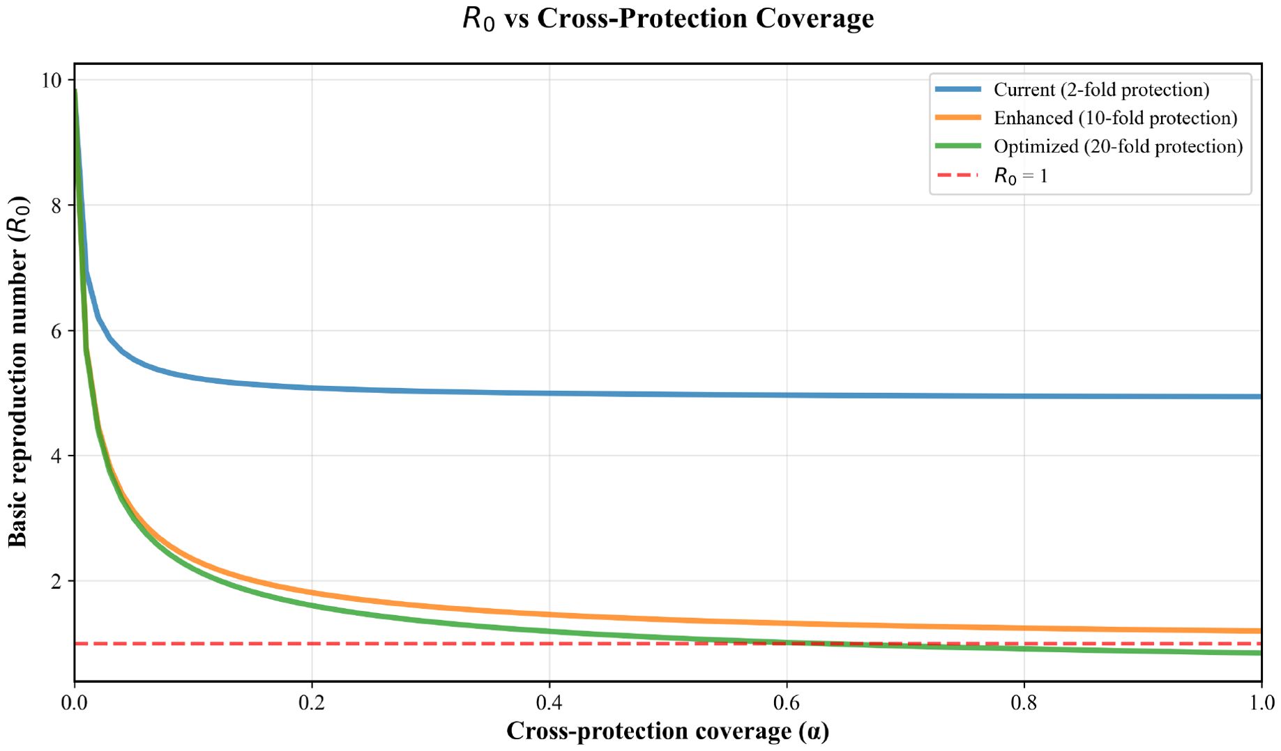
Figure 8. Basic reproduction number (R₀) as a function of cross-protection coverage (α) across three implementation scenarios.

Figure 3 confirms the analytical prediction of backward bifurcation under 20-fold protection (Scenario C). The endemic equilibrium (solid blue curve) exhibits a fold point that delimits a bistable region where a stable endemic state coexists with the DFE (green) even when R₀< 1. Increasing the roguing rate σ shifts the fold point to lower coverage values α, shrinking the bistable region. The dashed orange segment is the unstable endemic branch separating the two attraction basins, implying hysteresis (see Figure 9): driving R₀ just below one is not sufficient for elimination unless the initial infection is small.

Figure 9

Figure 9. For the same α value, the final equilibrium depends on where it is started: hysteresis behavior in backward bifurcation system.

5.3.2 Hysteresis effects

In Scenario C, we demonstrate hysteresis effects characteristic of backward bifurcation, see Figure 9.

1. Forward path: Gradually increasing α from 0 to 1 shows discontinuous jump from high to low endemic levels at α ≈ 0.7

2. Reverse path: Decreasing α from 1 to 0 shows discontinuous jump from low to high endemic levels at α ≈ 0.6

3. Hysteresis loop: The system exhibits different steady states depending on the direction of parameter change

This has important implications. Even with highly effective cross-protection, reducing coverage below critical thresholds can lead to sudden disease resurgence.

5.4 Threshold analysis and control implications

5.4.1 Critical coverage requirements

We define the baseline endemic level as the unique endemic equilibrium under Scenario A with no cross-protection, i.e. α = 0, using the Table 4 parameters. In this case Y* = U* = 0, and the plant–vector (X, Z, S, I) sustains transmission. Numerically we obtain

$$X*\approx 199.7, Z*\approx 574.3, S*\approx 15.8, I*\approx 150.9$$

Hence, the baseline scenario yields approximately 574.3 infected plants Z* + U*, and baseline infected vectors are I* ≈ 150.9. We express percent disease reduction relative to this baseline as

$$\text{Reduction}(\alpha )=\frac{{(Z^{*}+U^{*})}_{\text{baseline}}-(Z^{*}+U^{*})(\alpha )}{{(Z^{*}+U^{*})}_{\text{baseline}}}\times 100\%$$

We next evaluate steady states for two representative coverage levels, α = 0.4 (moderate) and α = 0.8 (high), under the three cross-protection scenarios. As shown analytically in Section 2.3, with Table 4 values the basic reproduction function R₀(α) does not cross 1 for A, B on α ∈ [0,1], while for Scenario C it crosses at α ≈ 6.3, thus elimination is only expected under sufficiently high coverage in Scenario C. The numerics below (Tables 6, 7) are consistent with these thresholds.

Table 6

Table 6. Steady-state infection by scenario and coverage.

Table 7

Table 7. Disease reduction in plants % reduction of Z* + U* vs baseline 574.3.

5.4.2 Cost-effectiveness considerations

Table 8 summarizes the coverage requirements for achieving specific disease reduction targets. While Scenario C illustrates the theoretical possibility, practical implementation costs increase significantly with effectiveness requirements. The analysis suggests

Table 8

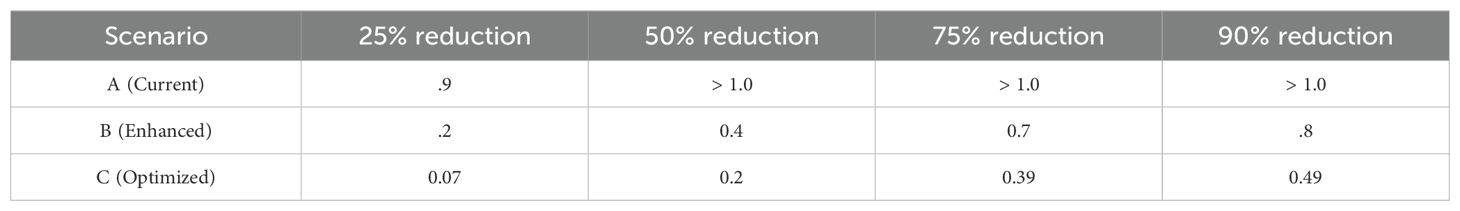
Table 8. Cross-protection coverage requirements for disease reduction targets (Here, > 1.0 indicate that the target reduction is not achievable even with complete coverage).

• Scenario A: Cost-effective only as supplementary strategy with minimal investment

• Scenario B: Represents optimal balance between effectiveness and implementation feasibility

• Scenario C: High implementation costs may limit practical adoption despite theoretical benefits

5.5 Comparative assessment

The numerical simulations provide a comprehensive view of cross-protection potential across implementation scenarios.

1. Current empirical evidence (Scenario A) supports cross-protection as a supplementary strategy that provides modest benefits when combined with traditional control methods.

2. Enhanced implementation (Scenario B) represents a realistic target where moderate improvements in effectiveness could substantially increase disease control benefits.

3. Optimized theoretical implementation (Scenario C) demonstrates the mathematical potential of cross-protection but requires significant advances in implementation technology.

The results emphasize that the effectiveness of cross-protection as a CMD control strategy critically depends on achieving implementation improvements beyond current field performance. The mathematical framework provides clear targets for research and development efforts aimed at optimizing cross-protection strategies.

5.6 Model limitations

Although the present model captures the key mechanisms driving cassava mosaic disease (CMD) dynamics, several simplifying assumptions were necessary to maintain analytical tractability. These include homogeneous host and vector populations, constant parameter values, and deterministic behavior. A detailed discussion of these limitations and potential model extensions—such as incorporating spatial heterogeneity, stochastic processes, or parameter uncertainty—is provided in Section 6.2.

5.7 Numerical methods

All numerical simulations were performed in Python 3.9 using SciPy 1.9.3. The ODE system (1)–(6) was integrated with the solve ivp routine employing the default RK45 (Runge–Kutta 4–5) adaptive solver. Relative and absolute tolerances were set to 10⁻⁶ and 10⁻⁸, respectively. Bifurcation diagrams were obtained by numerical continuation in the control parameter α, computing endemic equilibria at each step by solving the quadratic (Equation 15) and verifying their stability through eigenvalue analysis of the Jacobian matrix. Sensitivity analysis via Latin Hypercube Sampling used scipy.stats.qmc.LatinHypercube with 10,000 samples and a fixed random seed (12345) to ensure reproducibility.

6 Discussion

The results presented above clarify how partial cross-protection, roguing, and other interventions interact to shape the epidemiological dynamics of cassava mosaic disease (CMD). In this section, we interpret these findings in the context of field-level management and explore their broader relevance to vector-borne crop diseases. First, we discuss the practical implications of the model outcomes and their potential validation with empirical data. We then outline the model’s limitations and propose extensions that could enhance its biological realism and general applicability.

6.1 Practical implications and validation

Cassava mosaic disease (CMD) remains one of the most serious constraints on cassava production across sub-Saharan Africa, where integrated management requires balancing farmer-level feasibility and epidemiological effectiveness. Our modeling framework translates theoretical results into actionable guidance for disease control. The analyses indicate that improving the quality of cross-protection (the degree to which mild strains reduce susceptibility) is far more effective than expanding coverage alone. In practice, this suggests prioritizing the selection and deployment of highly protective mild strains, accompanied by regular monitoring of their efficacy in the field. The strong influence of roguing rate identified in the sensitivity analysis underscores the continued value of prompt removal of symptomatic plants to suppress inoculum sources.

To support real-world application, model outputs such as equilibrium prevalence, threshold roguing rates, and required protection efficacy can be directly compared with field survey or trial data. For example, existing CMD monitoring networks that record infection prevalence by cultivar and location could supply the empirical values needed to calibrate or test model predictions. This linkage enables the model to serve as a decision-support tool—helping extension programs to evaluate whether current intervention intensities are sufficient to push CMD below its persistence threshold.

Complexity versus usefulness. Allowing partial protection increases complexity only minimally: we retain the same six compartments and introduce no extra states, while distinguishing β₂ ≠ β₁ and β₄ ≠ β₃ and treating α as a bifurcation/implementation parameter. This preserves closed-form expressions (e.g., the two-cycle form of R₀) and low-cost computation, yet yields decision value by supporting threshold maps and trade-off analyses between coverage and roguing under empirically grounded (β₂, β₄).

Integration with field data. To operationalize these findings, we can calibrate key parameters with routine field measurements and targeted trials: (β₁, β₃) from vector–plant contact and infection rates (trap counts with plant inspections), (β₂, β₄) from challenge–inoculation experiments comparing protected versus unprotected plants (residual transmission fractions q₂ = β₂/β₁, q₄ = β₄/β₃), σ from roguing compliance logs, γ from insecticide bioassays, µ from life-table or mark–release–recapture data, and (α, α₁, K, ω, δ) from agronomic records and adoption/coverage surveys. We can fit the model via likelihood or Bayesian inference, use LHS/PRCC to prioritize influential parameters and quantify uncertainty, and validate out of sample against (i) time series of prevalence (Z+U)/K, (ii) observed elimination thresholds in σ or α, and (iii) post–intervention changes in R₀(α, σ). Mild–strain cross-protection (reducing β₂, β₄) complements host resistance (lowering β₁, β₃) and vector management (raising µ+γ); jointly, these levers reduce the coverage required for elimination, shift the fold to smaller α, and shrink the bistable region, thereby lowering hysteresis risk.

6.2 Model limitations and extensions

While the present framework captures the main transmission pathways and partial cross-protection dynamics of cassava mosaic disease (CMD), several simplifying assumptions limit its scope. The model assumes homogeneous host and vector populations with constant parameters and deterministic behavior. In practice, cassava fields exhibit spatial heterogeneity in planting density, cultivar composition, and whitefly movement, which can create localized infection clusters and temporal fluctuations. Future extensions could incorporate spatial structure or stochastic components to represent these sources of variability more realistically.

Parameter uncertainty also constrains the current analysis. Some epidemiological parameters—such as protection efficacy, vector transmission rates, and roguing efficiency—vary across regions and cultivars. Field surveys and controlled experiments could be used to refine these estimates and improve model calibration. In addition, non-dimensional reformulation of the equations could reveal scale-independent threshold quantities (see (Oh, 2025)), facilitating comparison across crop systems.

In practice, mild-strain inoculation can operate synergistically with host resistance and vector management by providing an additional biological barrier to severe-strain invasion, thereby stabilizing low-infection equilibria even under moderate vector pressure. Future work should integrate this modeling framework with empirical field data—particularly longitudinal CMD incidence and vector abundance—to refine parameter estimates (β₂, β₄, σ) and validate the predicted thresholds for successful cross-protection deployment.

Because the framework is mechanistic and modular, it can readily be adapted to other vector-borne crop diseases where protective interference or strain competition occurs—for example, citrus tristeza, yam mosaic, or grapevine fanleaf virus. Incorporating such extensions would broaden the model’s relevance and provide a unified mathematical basis for evaluating management strategies in diverse agro-ecosystems.

A natural next step is to incorporate spatial heterogeneity and vector movement explicitly into the model framework. Our subsequent work (Oh, 2025) develops a reaction–advection–diffusion system that extends the present vector–host formulation to heterogeneous landscapes, derives an explicit wave-speed predictor, and verifies linear determinacy through numerical traveling-wave simulations. That spatial framework connects the local reproduction number R₀ to regional invasion speeds and highlights how spatial variability and advection modify cross-protection outcomes.

7 Conclusion

This study developed a deterministic host–vector model to evaluate the role of partial cross-protection in the management of cassava mosaic disease (CMD). Analytical and numerical results revealed that cross-protection can generate backward bifurcation, such that reducing the basic reproduction number below one may still be insufficient for disease elimination. Sensitivity and uncertainty analyses showed that protection efficacy and roguing rate are the dominant factors determining long-term CMD prevalence, highlighting their importance as management levers. Simulations demonstrated that field-level protection of only moderate quality (≈ 2-fold reduction in susceptibility) provides limited benefit, whereas optimized protection (≥ 20-fold) could enable near-elimination even at partial coverage.

By linking nonlinear epidemiological thresholds with practical interventions, the model provides a quantitative tool for assessing CMD control strategies. The analysis also emphasizes that the quality of protection and efficiency of roguing are as critical as coverage levels and should be considered jointly in sustainable CMD management programs. The general structure of the model allows straightforward adaptation to other vector-borne crop diseases involving protective interference, such as citrus tristeza or grapevine fanleaf virus.

Building on the current deterministic framework, our subsequent study (Oh, 2025) introduces a spatially explicit extension incorporating diffusion, advection, and landscape heterogeneity. That formulation connects local epidemic thresholds with spatial spread rates, offering a complementary perspective on CMD management across heterogeneous agro-ecosystems.

Data availability statement

The original contributions presented in the study are included in the article/supplementary material. Further inquiries can be directed to the corresponding author.

Author contributions

MO: Conceptualization, Data curation, Formal analysis, Investigation, Methodology, Resources, Software, Supervision, Validation, Visualization, Writing – original draft, Writing – review & editing. MG: Conceptualization, Data curation, Formal analysis, Investigation, Methodology, Software, Writing – original draft.

Funding

The author(s) declared that financial support was received for this work and/or its publication.

Acknowledgments

The authors thank the reviewers for their insightful and constructive comments, which improved the clarity and rigor of this manuscript.

Conflict of interest

The authors declare that the research was conducted in the absence of any commercial or financial relationships that could be construed as a potential conflict of interest.

Generative AI statement

The author(s) declare that no Generative AI was used in the creation of this manuscript.

Any alternative text (alt text) provided alongside figures in this article has been generated by Frontiers with the support of artificial intelligence and reasonable efforts have been made to ensure accuracy, including review by the authors wherever possible. If you identify any issues, please contact us.

Publisher’s note

All claims expressed in this article are solely those of the authors and do not necessarily represent those of their affiliated organizations, or those of the publisher, the editors and the reviewers. Any product that may be evaluated in this article, or claim that may be made by its manufacturer, is not guaranteed or endorsed by the publisher.

References

Anggriani N., Supriatna A. K., and Sidarto K. A. (2020). Optimal control of plant disease model with roguing, replanting, curative, and preventive treatment. J. Physics: Conf. Ser. 1657, 012040. doi: 10.1088/1742-6596/1657/1/012050

Crossref Full Text | Google Scholar

Bokil V. A., Allen L. J. S., Jeger M. J., and Lenhart S. (2016). Optimal control of a vectored plant disease model for a crop with continuous replanting. J. Biol. Dynamics 13, 325–353. doi: 10.1080/17513758.2019.1622808

PubMed Abstract | Crossref Full Text | Google Scholar

Castillo-Chavez C. and Song B. (2004). Dynamical models of tuberculosis and their applications. Math. Biosci. Eng. 1, 361–404. doi: 10.3934/mbe.2004.1.361

PubMed Abstract | Crossref Full Text | Google Scholar

Chan M. S. and Jeger M. J. (1994). An analytical model of plant virus disease dynamics with roguing and replanting. J. Appl. Ecol. 31, 413–427. doi: 10.2307/2404439

Crossref Full Text | Google Scholar

Chikoti P. C., Mulenga R. M., Tembo M., and Sseruwagi P. (2019). Cassava mosaic disease: A review of a threat to cassava production in Zambia. J. Plant Pathol. 101, 467–477. doi: 10.1007/s42161-019-00255-0

PubMed Abstract | Crossref Full Text | Google Scholar

Diekmann O. and Heesterbeek J. A. P. (2000). Mathematical epidemiology of infectious diseases: model building, analysis and interpretation (New York: Wiley).

Google Scholar

Fulton R. W. (1986). Practices and precautions in the use of cross protection for plant virus disease control. Annu. Rev. Phytopathol. 24, 67–81. doi: 10.1146/annurev.py.24.090186.000435

Crossref Full Text | Google Scholar

Gal-On A. and Shiboleth Y. M. (2006). “Cross-protection,” in Natural resistance mechanisms of plants to viruses (Springer, Dordrecht), 261–288.

Google Scholar

Gilligan C. A. (2008). Sustainable agriculture and plant diseases: An epidemiological perspective. Philos. Trans. R. Soc. B: Biol. Sci. 363, 741–759. doi: 10.1098/rstb.2007.2181

PubMed Abstract | Crossref Full Text | Google Scholar

Jeger M. J., Holt J., Reynolds F. D., and Chan M. S. (2004). Epidemiology of insect-transmitted plant viruses: Modelling disease dynamics and control interventions. Physiol. Entomology 29, 291–304. doi: 10.1111/j.0307-6962.2004.00394.x

Crossref Full Text | Google Scholar

Komar V., Vigne E., Demangeat G., and Femaire O. (2008). Plant cross-protection as a control strategy against grapevine fanleaf virus in naturally infected vineyards. Plant Dis. 92, 1689–1694. doi: 10.1094/PDIS-92-12-1689

PubMed Abstract | Crossref Full Text | Google Scholar

Luo L., Gao S., Ge Y., and Luo Y. (2017). Transmission dynamics of a Huanglongbing model with cross-protection. Adv. Difference Equations 2017, 355. doi: 10.1186/s13662-017-1392-y

Crossref Full Text | Google Scholar

Oh M. (2025). Effective transport and minimal invasion speed in a vector–host model of cassava mosaic disease with partial cross-protection. SSRN preprint. Available online at: http://ssrn.com/abstract=5675995.

Google Scholar

Owor B., Legg J. P., Okao-Okuja G., Obonyo R., Kyamanywa S., and Ogenga-Latigo M. W. (2004). Field studies of cross protection with cassava mosaic geminiviruses in Uganda. J. Phytopathol. 152, 243–249. doi: 10.1111/j.1439-0434.2004.00837.x

Crossref Full Text | Google Scholar

Patil B. L. and Fauquet C. M. (2009). Cassava mosaic geminiviruses: Actual knowledge and perspectives. Mol. Plant Pathol. 10, 685–701. doi: 10.1111/j.1364-3703.2009.00559.x

PubMed Abstract | Crossref Full Text | Google Scholar

Shuai Z. and van den Driessche P. (2013). Global stability of infectious disease models using Lyapunov functions. SIAM J. Appl. Math. 73, 1513–1532. doi: 10.1137/120876642

Crossref Full Text | Google Scholar

Zhang X. S. and Holt J. (2001). Mathematical models of cross protection in the epidemiology of plant-virus diseases. Phytopathology 91, 924–931. doi: 10.1094/PHYTO.2001.91.10.924

PubMed Abstract | Crossref Full Text | Google Scholar

Zhou C. and Zhou Y. (2012). Strategies for viral cross protection in plants. In. Methods Mol. Biol. 894, 69–81. doi: 10.1007/978-1-61779-882-5_5

PubMed Abstract | Crossref Full Text | Google Scholar