 Taichi Tomono
 Satoshi Hara1
- 1Department of Reasoning for Intelligence, The Institute of Scientific and Industrial Research, Osaka University, Ōsaka, Japan
- 2AI Solution Unit, Technology Research Laboratory, Shimadzu Corporation, Kyoto, Japan
- 3Shimadzu Analytical Innovation Research Laboratories, Osaka University, Ōsaka, Japan
- 4Life Science Business Department, Analytical and Measuring Instruments Division, Shimadzu Corporation, Kyoto, Japan
Mass spectrometry (MS) is a powerful analytical method used for various purposes such as drug development, quality assurance, food inspection, and monitoring of pollutants in the environment. In recent years, with the active development of antibodies and nucleic acid-based drugs, impurities with various modifications are produced. These can lead to a decrease in drug stability, pharmacokinetics, and efficacy, making it crucial to differentiate these impurities. Previously, attempts have been made to estimate the monoisotopic mass and ion amounts in the spectrum generated by electrospray ionization (ESI). However, conventional methods could not explicitly estimate the number of constituents, and discrete state evaluations, such as the probability that the number of constituents is k or k+1, were not possible. We propose a method where, for each possible number of constituents in the sample, mass spectrometry is modeled using parameters like monoisotopic mass and ion counts. Using Simulated Annealing, NUTS, and stochastic variational inference, we determine the parameters for each constituent number model and the maximum posterior probability. Finally, by comparing the maximum posterior probabilities between models, we select the optimal number of constituents and estimate the monoisotopic mass and ion counts under that scenario.
1 Introduction
Mass Spectrometry (MS) is a powerful analytical technique used for various purposes such as drug development and quality assurance, food inspection, and monitoring of pollutants in the environment. In recent years, with the active development of antibodies and nucleic acid drugs, impurities with different modifications are produced. These can cause a decrease in the stability of the drug, its pharmacokinetics, and its efficacy (Weinberg et al., 2005; Sanghvi, 2011; Pecori et al., 2022; Tamara et al., 2022). Therefore, it is crucial in drug development and quality assurance to distinguish these multiple impurities in pharmaceuticals and take measures against them. Moreover, if we know the monoisotopic mass of the constituents, it can provide valuable information for considering the cause of impurity generation, and if the ion amounts of the constituents are known, it helps estimate the effect of the impurity.
However, in current mass spectrometry, it is generally difficult to directly distinguish impurities in targets of middle molecules or higher that have slight modifications, and to estimate the correct number of constituents and their monoisotopic mass and ion amounts. This challenge arises because separating such impurities using conventional chromatography methods is problematic. Furthermore, the MS spectra become complex due to the isotopes in the target constituent. Especially with the most used ionization method, Electrospray Ionization (ESI), more complex spectra are produced because it creates multivalent ions, leading to many interpretations and degrees of freedom, making analysis even more challenging.
While increasing hardware resolution can differentiate slight differences between isotopes and modifications, methods like FT-ICR (Fourier Transform Ion Cyclotron Resonance), which have high resolution, require massive equipment and substantial costs, making it inconvenient to handle. Thus, it is preferable to analyze with devices that can be managed in general labs, such as Triple-Quadrupole-MS and Quadrupole -Time-of-Flight-MS(Q-TOF-MS).
Therefore, there is active research in approaching signal analysis through software. Various attempts have been made to estimate mass from mass spectrometer data. Simple methods to derive m/z lists from spectra include wavelet transformation (Zhang et al., 2009). Recently, peak detection algorithms have been developed that combine continuous wavelet transformation (CWT) and image processing (Deng et al., 2021). This method applies image segmentation to CWT coefficients, creating masks, and combining them with CWT maximum values to improve peak detection ROC (receiver operating characteristic) curve. Such techniques are useful for resolving close mass constituents in spectra measured with low molecules, which have a relatively narrow isotope distribution, or when ionized with methods producing simple charge distributions like EI (electron ionization) or MALDI (matrix-assisted laser desorption ionization). However, for spectra of middle to high molecules with a wide isotope distribution, especially those generated by ESI, which produce multivalent ions with a charge distribution, distinguishing the monoisotopic mass of interest becomes challenging.
For charge deconvolution and deisotoping from multivalent ion spectra, a lot of algorithms such as heuristic gaussian fitting using nonlinear least squares minimization (Dasari et al., 2009) have been proposed. The ReSpect algorithm using the Max Entropy method (Ferrige et al., 1992) has been long used (Zhang and Alecio, 1998; Tranter, 2000; Ferrige et al., 2003). This algorithm integrates m/z lists based on charge distribution constraints, enabling the determination of monoisotopic mass. However, ReSpect cannot explicitly estimate the number of constituents in the spectrum, and it cannot evaluate discrete states, like the probability that there are
Recently, new methods like UniDec using Bayesian deconvolution have emerged (Marty et al., 2015; Marty, 2020). UniDec adopts a unique algorithm similar to the Richardson-Lucy method (Richardson, 1972; Lucy, 1974) and is faster than ReSpect. However, its iterative method to approximate the observed data by a convoluted spectrum does not resolve the issue of not being able to evaluate the probability of a certain number of constituents.
In this paper, we newly propose a method to select the optimal number of constituents by comparing the probability of each constituent count, and to estimate the monoisotopic mass and ion counts under that condition. This can suggest the presence of impurities in pharmaceuticals, assist in the search for better synthesis conditions for middle to high molecular pharmaceuticals, and be useful for quality assurance in factories. For this study, we target Time-of-Flight mass spectrometers, which are frequently used in drug development due to their high sensitivity and resolution.
2 Proposed method
2.1 Analytical method framework
First, we model the mass spectrometry system based on parameters like the mass and charge of each constituent, assuming a certain number of constituents in the sample. Here, a constituent is defined as a substance with a specific monoisotopic mass. We then perform a MAP (Maximum A Posteriori) estimation of these parameters from the observed spectrum. By comparing the maximum posterior probability in models with different numbers of constituents, we determine the model with the most appropriate number of constituents.
However, this model has a large dimensionality of the number of constituents multiplied by 6. Moreover, the posterior probability for one of the parameters, the monoisotopic mass, is flat over a large portion of the search space and has several sharp peaks locally. Hence, gradient-based methods are not suitable for this case due to anticipated gradient vanishing. Therefore, to estimate the parameters, we combine the No-U-Turn Sampler (NUTS (Hoffman and Gelman, 2014), a type of Markov Chain Monte Carlo (MCMC), with Simulated Annealing (Kirkpatrick, Gelatt, and Vecchi, 1983).
The purpose of using Simulated Annealing is to introduce a temperature parameter. By selecting a high-temperature exploration parameter distribution, we can actively explore parameters even in areas where the posterior probability is flat or has sharp peaks. This ensures a broader search across the parameter space, reducing the chance of overlooking the global solution and getting trapped in local minima.
Furthermore, NUTS can explore parameters sparsely in areas with small gradients and can explore parameters in detail in areas with large gradients. Thus, introducing NUTS allows efficient exploration of the vast, high-dimensional parameter space.
On the other hand, while MCMC is good at searching for global solutions, it does not always reach the optimal solution within a certain number of search steps. Therefore, we use the parameters with the highest posterior probabilities obtained from NUTS and Simulated Annealing as initial values and apply stochastic variational inference. By doing this, we search for the optimal parameter where the posterior probability is maximized in the vicinity of that initial value, aiming to improve the accuracy of parameter estimation.
However, simultaneously searching for parameters for all possible numbers of constituents leads to a curse of dimensionality, where the search space explosively expands as the number of constituents increases, potentially reducing search efficiency and accuracy. To avoid this problem, we sequentially increase the number of constituents from
To balance the complexity of the model (number of constituents) and its fit (loss against the data), in addition to the prior distribution of each parameter, we introduce a prior distribution for the number of constituents. We also incorporate a prior distribution on the differences between the monoisotopic masses of multiple constituents. For analytical purposes, we have defined a single constituent as a substance with a distinct monoisotopic mass, thereby ensuring that their masses do not mutually take the same value. When seeking to separate isomers, it is essential to integrate other techniques such as fragmentation, ion mobility spectrometry, and chromatography, in addition to the proposed method. We first construct a model with
Next, we construct a model with
Subsequently, we seek the maximum posterior probability for each model with constituent numbers up to the upper limit
Finally, we compare the maximum posterior probabilities corresponding to each model with different numbers of constituents. We select the model with the highest probability and obtain the estimates for the monoisotopic masses and ion counts.
2.2 Physical model of mass spectrometers
In a time-of-flight mass spectrometer, the relationship between time of filght
The actual signal obtained is a convolution of the delta function
Reflecting these variances in time of flight and detector response intensity, the response
The mass
However, this model becomes too complex for Bayesian inference due to its large number of parameters
Consequently, the mass distribution of constituent j can be represented by a binomial distribution based on the monoisotopic mass as a reference, where
Considering that constituent j contains up to
If the ion counts are sufficiently large, it can be approximated as:
Noise in the time-of-flight mass spectrometer is known to be stationary and follows a normal distribution based on preliminary experiments. It is known that the thermal noise of detection circuits in such as mass spectrometers follows a normal distribution (Johnson, 1928), suggesting that in this case, thermal noise is the dominant factor in overall noise. Therefore, the noise to be added to the entire spectrum is represented as
Considering these, the conclusive spectrum combined with the multiple spectra of single constituent is represented as:
2.3 Bayesian estimation of number of constituents and parameters
When the observation data from the mass spectrometer
Here, in addition to the prior distribution of each parameter (uniform distribution), we incorporate a regularization term,
To determine the appropriate number of constituents
Furthermore, we define a constituent by its unique monoisotopic mass. Therefore, if the estimated values of the monoisotopic mass parameters of multiple constituents are the same in the algorithm, the count of constituents will not be accurate. Here, we define the logarithmic prior distribution (regularization term)
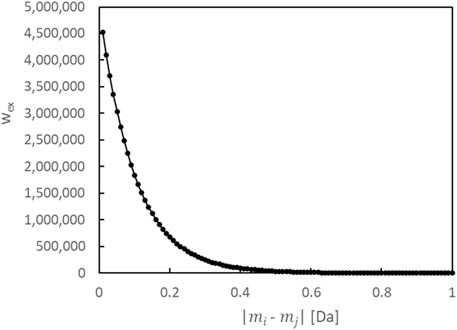
FIGURE 1. Characteristics of the regularization term
Here, by substituting the parameter
Here,
To obtain the maximum posterior probability and parameters
2.4 Parameter exploration and optimization
From the posterior probability distribution
After executing MCMC, the parameters of the maximum posterior probability obtained are inherited as initial values, and optimization of the parameters is performed using Stochastic Variational Inference [SVI (Kingma and Max, 2013; Wingate and Weber, 2013; Ranganath et al., 2014)]. For more details, please refer to the Supporting Material.
2.5 Workflow for inferring constituents in a sample
The overall picture of the workflow to determine the optimal parameters and posterior probability for each assumed number of constituents from the observational data of the mass spectrometer is as shown in Figure 2.
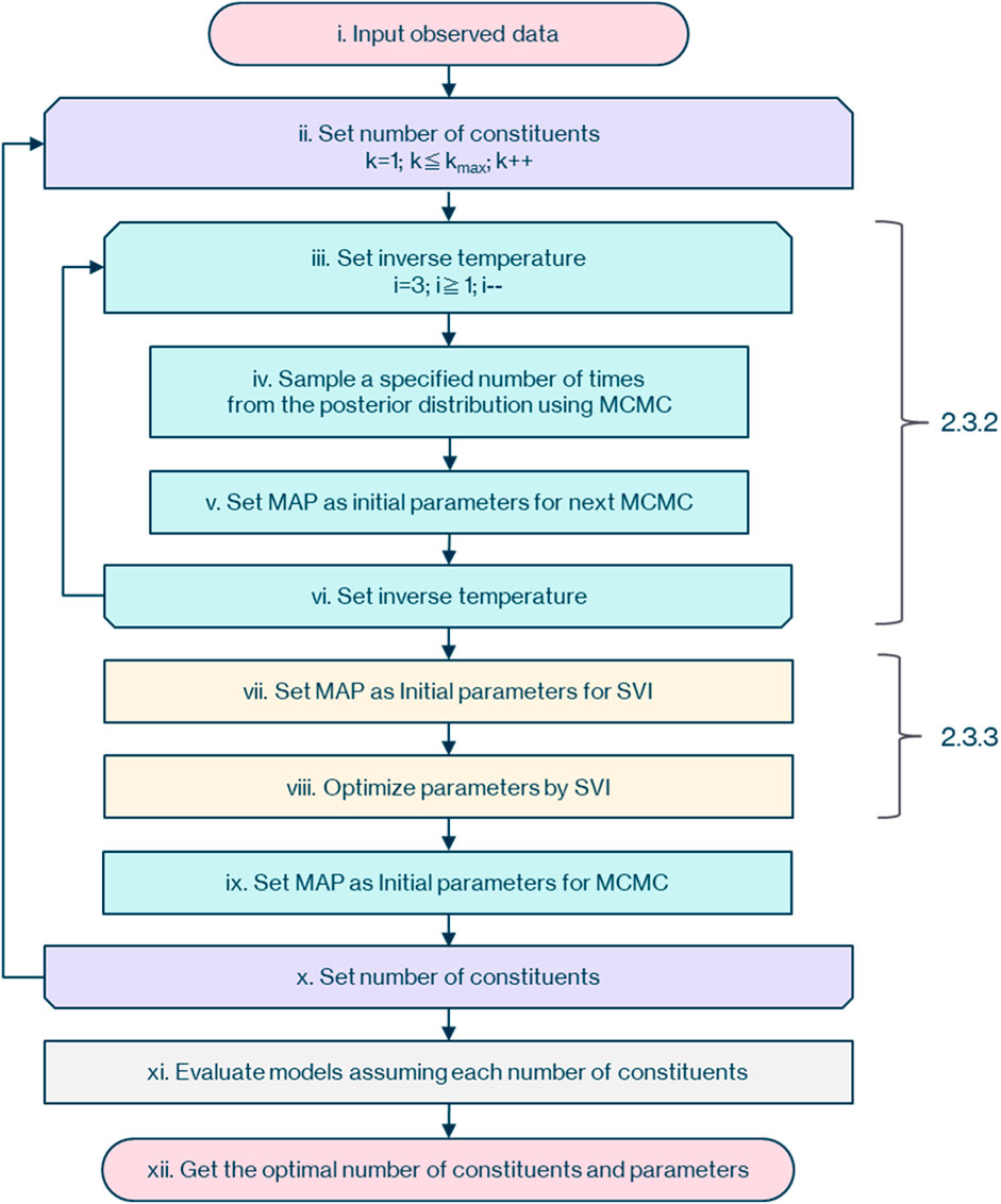
FIGURE 2. Inference process overall workflow.
First, as described in 2.3.1, (i) input the observational data of the mass spectrometer with dimensions of flight time and ion counts. Then (ii) assume that the number of constituents,
Next, as described in 2.3.2, (iv) sample
As described in 2.3.3, (vii) set the parameter of the maximum posterior probability obtained by MCMC as the initial value for SVI. Then (viii) optimize the parameters with SVI, and (ix) set the parameter of the maximum posterior probability obtained by SVI as the initial value for the next MCMC.
Following 2.3.1, increase the number of constituents,
3 Results
3.1 Validation environment
The specifications of the PC used for verifying the proposed method, as well as the software versions, are detailed in Table 1. The proposed method handles data with 1 million dimensions along the time axis, requiring a large memory size. Additionally, to rapidly explore a wide 6-dimensional parameter space using MCMC, the high-speed probabilistic programming library, NumPyro, along with its compatible CUDA and GPU, were used.
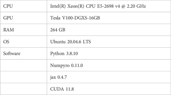
TABLE 1. Validation environment.
3.2 Creation of simulation data for validation
Based on the nucleic acid drug Fomivirsen (Perry and Balfour, 1999) (ID: A), four impurity constituents with modified base sequences were added, and spectra for a total of five constituents were generated via simulation. Specific values are as per Table 2. This enables the replication of a system where the principal constituent’s isotopic distribution and the impurity spectra are mixed.
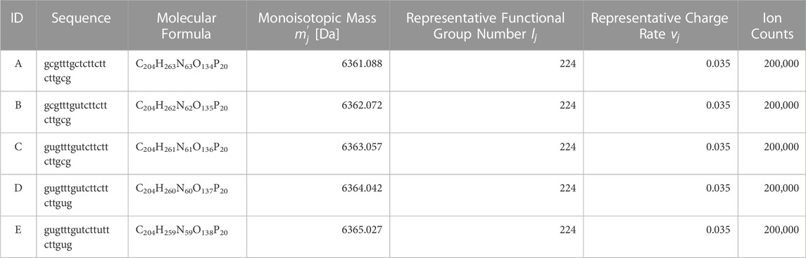
TABLE 2. Settings for constituent spectrum generation.
Ion counts for each constituent were set at 20,000. To facilitate the interpretation of results and to ensure that the algorithm treats each constituent fairly, we will conduct evaluations using a 1:1 concentration ratio for each component in the proposed method. The atomic counts
The procedure involved sampling from the multinomial distribution represented by Eqs 3 and 4 20,000 times (total incoming ion counts) for each constituent. Subsequently, spectra were formed following the procedures in Eqs 2 and 7.
The mutation from C (Cytosine) to U (Uracil) is called deamination and is generated in the synthesis process due to solvent conditions and thermal stress (Stavnezer, 2011; Gao, Choudhry, and Cao, 2018).
The spectra of the generated single constituents A to E were combined according to Eq. 9 in the 15 combinations listed in Table 3. This allows for a comprehensive combination of 2-3 constituents based on constituent A, as well as an evaluation of each individual constituent. We use these as test data.
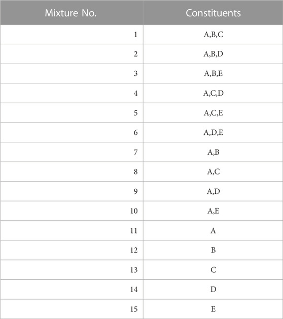
TABLE 3. Combinations of constituents when generating spectra.
3.3 Evaluation of constituent count estimation accuracy
The results of estimating the number of constituents in the spectra of the test data (Mixture No.1∼15) using our proposed method are as shown in Table 4. The values within the table represent the negative logarithm of the maximum posterior probability in the model of constituent count k. Therefore, the smallest value should be selected.
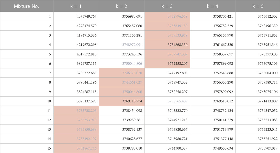
TABLE 4. Negative logarithm of the maximum posterior probability assuming each constituent count (Orange background indicates the true number of constituents, blue text indicates the minimum value across models).
By choosing the most suitable number of constituents based on this criterion, the success rate for estimating the true number of constituents was 80% (12/15). Additionally, the presence or absence of impurities (distinguishing between k = 1 and k≧2) could be determined with 100% accuracy. We believe this is sufficient as a standard for recognizing the presence and number of impurities in pharmaceuticals and taking appropriate measures.
3.4 Accuracy of parameter estimation with maximum posterior
The optimal monoisotopic masses and ion counts estimated in the model where the posterior probability is maximum for each test data are shown in Table 5. The monoisotopic mass had an average error of 1.348 Da and a maximum error of 4.931 Da. This is insufficient to determine how many mutations have occurred, making it unsuitable for examining the cause of impurity generation with a difference of 1 Da. Regarding the ion counts, there was an average error of 4% and a maximum error of 82%. For instance, the standards for total desamido impurity and total impurities in injectable glucagon are 14% or less and 31% or less, respectively (Bao et al., 2022). Therefore, the accuracy of the ion count estimation in the proposed method is insufficient to estimate the impact of impurities.
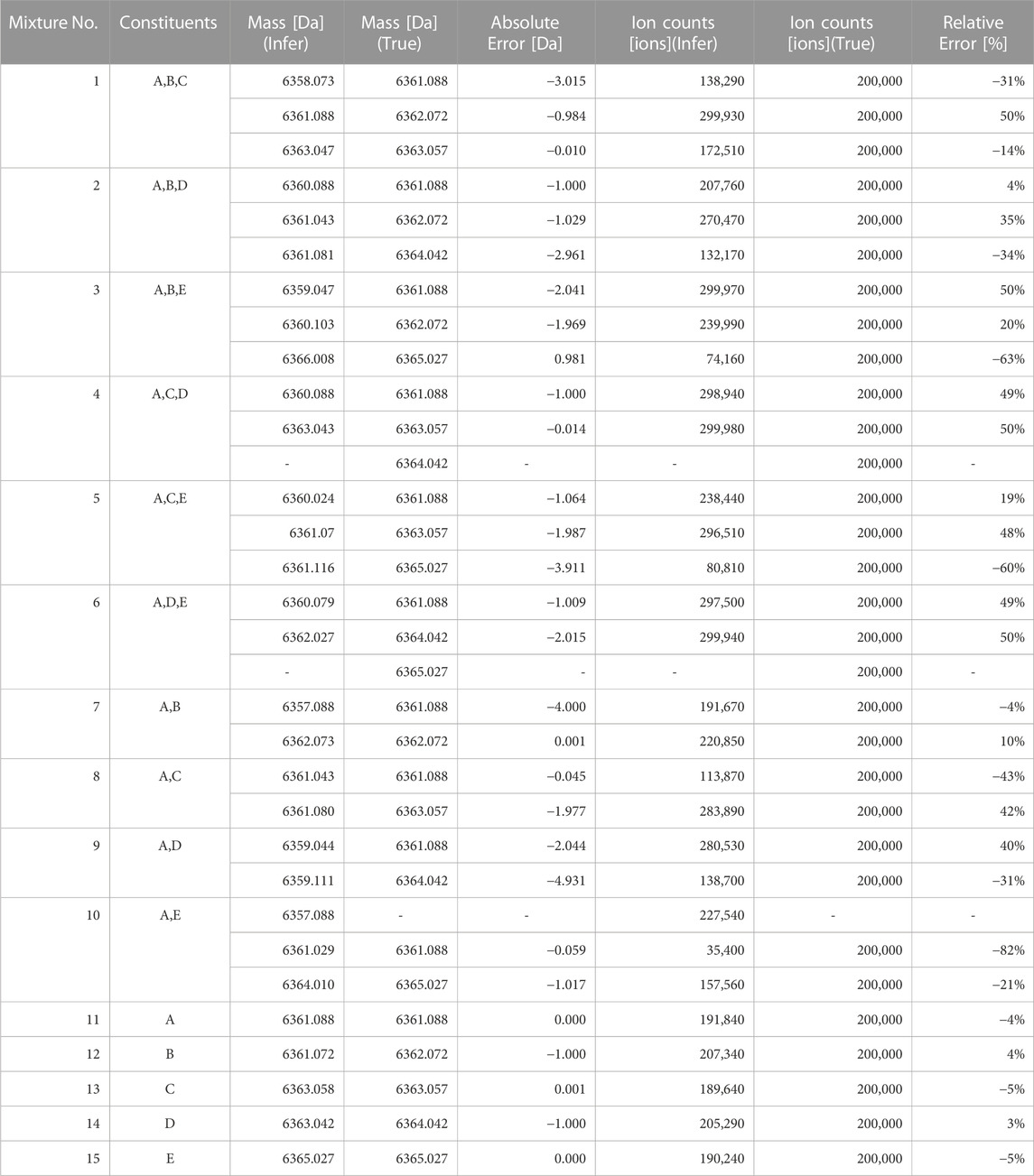
TABLE 5. Optimal monoisotopic masses and ion counts of the model with the maximum posterior probability.
For reference, a comparison between the spectra reconstructed from the estimated parameters and the original signal is shown in Figure 3. The overall view in (a) represents the charge distribution, and the enlarged view in (b) represents the isotopic distribution. From these results, it is clear that the spectrum we generated closely matches the observed data. Despite the spectra matching, errors in parameter estimation occurred because of the high degree of freedom in isotopic parameters that trade-off with monoisotopic mass. Even if the monoisotopic mass was lower than the true value, by increasing the representative atomic number
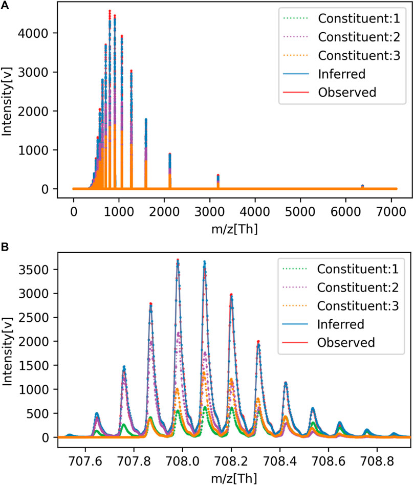
FIGURE 3. Comparison of observed and estimated spectra for Mixture No. 1. (A) Overall view, (B) Enlarged view.
Also, the estimated ion counts of each constituent showed errors of up to 82% from the true values. This is presumed to be due to the trade-off relationship between the ion counts of each constituent, with a decrease in the ion count of one constituent being compensated by an increase in another. This is further supported by the fact that the average error in ion counts settles at 4%.
3.5 Comparison with UniDec
Deconvolution of the test data was performed using the existing method, UniDec as well. The results of deconvolution for each observed spectrum by UniDec are shown in Table 6. According to these results, the accuracy for the correct number of constituents was 13% (2/15). This is presumed to be because the UniDec algorithm, which obtains the number of constituents after multiple iterations of deconvolution, does not necessarily guarantee the number of constituents. Please note that this use of UniDec to determine the number of constituents is not its intended application.
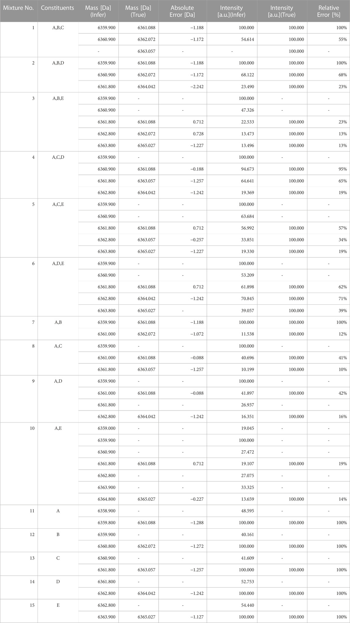
TABLE 6. Deconvolution results for each observed spectrum by UniDec.
For the verification above, we used UniDec (Version 6.0.2). The particularly set parameters during this verification are shown in Table 7. The Mass Range was set to the same range as the proposed method, and Sample Mass Every (Da) was set to 0.1 to sufficiently detect impurities with a difference of 1 Da. For parameters not mentioned, default values were used.
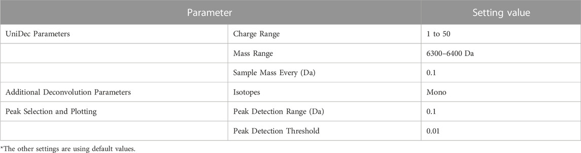
TABLE 7. UniDec setting parameters.
4 Discussion
Using NUTS, Simulated Annealing, and stochastic variational inference, we estimated parameters such as monoisotopic masses from observed data, and were able to choose the correct number of constituents with a higher probability than existing methods. This is thought to be due to the fact that we created models for each number of constituents, allowing for the comparative evaluation and selection of models for each number of constituents. This made it possible to suggest the presence of impurities in pharmaceuticals, which is useful for searching for better synthesis conditions for middle to high molecular weight pharmaceuticals, and for quality assurance in factories.
On the other hand, as shown in Table 5, the estimated monoisotopic mass had a maximum error of 4.931Da from the true value. This is thought to be due to the trade-off relationship between the monoisotopic mass
Furthermore, it took about 50 h for deconvolution assuming 5 constituents per data. This is long compared to the few seconds to a few minutes processing time of UniDec. Also, this processing time is expected to increase almost linearly with the assumed number of constituents. Therefore, it is expected to take a long time when analyzing samples with many constituents, such as serum or environmental samples. A possible countermeasure to this problem is to divide the monoisotopic mass space into mini-batches and perform parallel calculations.
5 Conclusion
We assumed multiple numbers of constituents in the sample and created a mass spectrometry model from parameters such as monoisotopic masses and ion counts. We then sought the maximum posterior probability in the model of each number of constituents against observed data using NUTS, Simulated Annealing, and stochastic variational inference. As a result, we were able to estimate the number of constituents with high accuracy. We were also able to estimate parameters such as monoisotopic masses and ion counts at the same time.
Future challenges include reducing computation time, improving mass accuracy, and improving ion count accuracy. Incorporating chromatography or ion mobility information, addressing more stringent concentration ratios between constituents (e.g., greater than 10:1), and adapting to complex samples with more constituents will be pursued to expand the applicability of this method.
Data availability statement
The raw data supporting the conclusion of this article will be made available by the authors, without undue reservation.
Author contributions
TT: Conceptualization, Investigation, Methodology, Project administration, Software, Validation, Visualization, Writing–original draft. SH: Writing–review and editing, Conceptualization. YN: Methodology, Software, Writing–review and editing. KT: Software, Writing–review and editing. JI: Writing–review and editing. TW: Conceptualization, Supervision, Writing–review and editing.
Funding
The author(s) declare that no financial support was received for the research, authorship, and/or publication of this article.
Acknowledgments
We extend our deepest gratitude to Yoshihiro Ueno, Yusuke Tagawa, Daisuke Okumura, and Daisuke Hiramaru for their advice and coordination on the project as a whole. We also thank Akira Noda and Yusuke Tamai for their insights on Bayesian estimation. Atsuhiko Toyama, Natsuyo Asano, Hiroaki Waki, Kiyoshi Ogawa, Hideaki Izumi, Masahiro Takebe, Takashi Kawabe, and Yusuke Tateishi for their advice on the needs and trends of mass spectrometers. Our appreciation extends to Makoto Yamada and Tomoyuki Oshiro for obtaining the single response waveforms of the detectors, to Masaru Nishiguchi and Hiroyuki Miura for providing samples, to Momoka Hayashida and Noriko Kato for offering insights on nucleic acid analysis, to Yuta Miyazaki for advice on noise characteristics, and to Tomoya Kudo for guidance on ion optics simulations.
Conflict of interest
Authors TT, YN, KT, and JI were employed by Shimadzu Corporation.
The remaining authors declare that the research was conducted in the absence of any commercial or financial relationships that could be construed as a potential conflict of interest.
Publisher’s note
All claims expressed in this article are solely those of the authors and do not necessarily represent those of their affiliated organizations, or those of the publisher, the editors and the reviewers. Any product that may be evaluated in this article, or claim that may be made by its manufacturer, is not guaranteed or endorsed by the publisher.
Supplementary material
The Supplementary Material for this article can be found online at: https://www.frontiersin.org/articles/10.3389/frans.2023.1301602/full#supplementary-material
References
Bao, Z., Cheng, Y. C., Luo, M. Z., and Zhang, J. Y. (2022). Comparison of the purity and impurity of glucagon-for-injection products under various stability conditions. Sci. Pharm. 90 (2), 32. doi:10.3390/scipharm90020032
Betancourt, M. (2017). A conceptual introduction to Hamiltonian Monte Carlo. ArXiv [Stat.ME]. Available at: http://arxiv.org/abs/1701.02434.
Boesl, U. (2017). Time-of-Flight mass spectrometry: introduction to the Basics. Mass Spectrom. Rev. 36 (1), 86–109. doi:10.1002/mas.21520
Dasari, S., Wilmarth, P. A., Reddy, A. P., Robertson, L. J. G., Nagalla, S. R., and David, L. L. (2009). Quantification of isotopically overlapping deamidated and 18O-labeled peptides using isotopic envelope mixture modeling. J. Proteome Res. 8 (3), 1263–1270. doi:10.1021/pr801054w
Deng, F., Li, H., Wang, R., Yue, H., Zhao, Z., and Duan, Y. (2021). An improved peak detection algorithm in mass spectra combining wavelet Transform and image segmentation. Int. J. Mass Spectrom. 465, 116601. doi:10.1016/j.ijms.2021.116601
Ferrige, A., Ray, S., Alecio, R., Ye, S., and Waddell, K. (2003). Electrospray-MS charge deconvolutions without compromise – an enhanced data reconstruction algorithm utilising variable peak modelling. Available at: https://positiveprobability.com/POSTERS/ASMS%202003.pdf.
Ferrige, A. G., Seddon, M. J., Green, B. N., Jarvis, S. A., Skilling, J., and Staunton, J. (1992). Disentangling electrospray spectra with maximum entropy. Rapid Commun. Mass Spectrom. RCM 6 (11), 707–711. doi:10.1002/rcm.1290061115
Gao, J., Choudhry, H., and Cao, W. (2018). Apolipoprotein B MRNA editing enzyme catalytic polypeptide-like family genes activation and regulation during tumorigenesis. Cancer Sci. 109 (8), 2375–2382. doi:10.1111/cas.13658
Hoffman, M. D., and Gelman, A. (2014). The No-U-turn sampler: adaptively setting path lengths in Hamiltonian Monte Carlo. J. Mach. Learn. Res. JMLR 15 (1), 1593–1623. doi:10.48550/arXiv.1111.4246
Johnson, J. B. (1928). Thermal agitation of electricity in conductors. Phys. Rev. 32 (1), 97–109. doi:10.1103/physrev.32.97
Kingma, D. P., and Max, W. (2013). Auto-encoding variational Bayes. ArXiv [Stat.ML]. Available at: http://arxiv.org/abs/1312.6114v11.
Kirkpatrick, S., Gelatt, C. D., and Vecchi, M. P. (1983). Optimization by simulated annealing. Science 220 (4598), 671–680. doi:10.1126/science.220.4598.671
Lucy, L. B. (1974). An iterative technique for the rectification of observed distributions. Astronomical J. 79, 745. doi:10.1086/111605
Marty, M. T. (2020). A universal score for deconvolution of intact protein and native electrospray mass spectra. Anal. Chem. 92 (6), 4395–4401. doi:10.1021/acs.analchem.9b05272
Marty, M. T., Baldwin, A. J., Marklund, E. G., Hochberg, G. K. A., Benesch, J. L. P., and Robinson, C. V. (2015). Bayesian deconvolution of mass and ion mobility spectra: from binary interactions to polydisperse ensembles. Anal. Chem. 87 (8), 4370–4376. doi:10.1021/acs.analchem.5b00140
Neal, R. (2011). “Handbook of Markov chain Monte Carlo,” in Chapter 5: MCMC using Hamiltonian Dynamics (United States: CRC Press).
Neath, A. A., and Cavanaugh, J. E. (2012). The bayesian information criterion: background, derivation, and applications. WIREs Comput. Stat. 4 (2), 199–203. doi:10.1002/wics.199
Pecori, R., Di Giorgio, S., Paulo Lorenzo, J., and Nina Papavasiliou, F. (2022). Functions and consequences of AID/APOBEC-Mediated DNA and RNA deamination. Nat. Rev. Genet. 23 (8), 505–518. doi:10.1038/s41576-022-00459-8
Perry, C. M., and Balfour, J. A. (1999). Fomivirsen. Drugs 57 (3), 375–380. discussion 381. doi:10.2165/00003495-199957030-00010
Ranganath, R., Gerrish, S., and Blei, D. (2014). “Black Box variational inference,” in Proceedings of the Seventeenth international conference on artificial intelligence and Statistics, edited by Samuel Kaski and Jukka corander, 33:814–22. Proceedings of machine learning research (Reykjavik, Iceland: PMLR).
Richardson, W. H. (1972). Bayesian-based iterative method of image restoration. J. Opt. Soc. Am. 62 (1), 55. doi:10.1364/josa.62.000055
Sanghvi, Y. S. (2011). A status update of modified oligonucleotides for chemotherapeutics applications. Curr. Protoc. Nucleic Acid Chem. 2011, 1–22. Chapter 4 (September): Unit 4.1. doi:10.1002/0471142700.nc0401s46
Schwarz, G. (1978). Estimating the dimension of a model. Ann. Statistics 6 (2), 461–464. doi:10.1214/aos/1176344136
Stavnezer, J. (2011). Complex regulation and function of activation-induced cytidine deaminase. Trends Immunol. 32 (5), 194–201. doi:10.1016/j.it.2011.03.003
Tamara, S., den Boer, M. A., and Heck, A. J. R. (2022). High-resolution native mass spectrometry. Chem. Rev. 122 (8), 7269–7326. doi:10.1021/acs.chemrev.1c00212
Weinberg, W. C., Frazier-Jessen, M. R., Wu, W. J., Weir, A., Hartsough, M., Keegan, P., et al. (2005). Development and regulation of monoclonal antibody products: challenges and opportunities. Cancer Metastasis Rev. 24 (4), 569–584. doi:10.1007/s10555-005-6196-y
Wingate, D., and Weber, T. (2013). Automated variational inference in probabilistic programming. ArXiv E-Prints, arXiv:1301.1299. Available at: https://doi.org/10.48550/arXiv.1301.1299.
Zhang, J., Gonzalez, E., Hestilow, T., Haskins, W., and Huang, Y. (2009). Review of peak detection algorithms in liquid-chromatography-mass spectrometry. Curr. Genomics 10 (6), 388–401. doi:10.2174/138920209789177638
Keywords: LC-MS, ESI, chemometrics, Bayesian inference, deconvolution, signal processing, nucleic-acid-drugs
Citation: Tomono T, Hara S, Nakai Y, Takahara K, Iida J and Washio T (2024) A Bayesian approach for constituent estimation in nucleic acid mixture models. Front. Anal. Sci. 3:1301602. doi: 10.3389/frans.2023.1301602
Received: 05 September 2023; Accepted: 14 December 2023;
Published: 08 January 2024.
Edited by:
Krzysztof Bernard Bec, University of Innsbruck, AustriaReviewed by:
Rui Vitorino, University of Aveiro, PortugalMarina De Gea Neves, University of Duisburg-Essen, Germany
Copyright © 2024 Tomono, Hara, Nakai, Takahara, Iida and Washio. This is an open-access article distributed under the terms of the Creative Commons Attribution License (CC BY). The use, distribution or reproduction in other forums is permitted, provided the original author(s) and the copyright owner(s) are credited and that the original publication in this journal is cited, in accordance with accepted academic practice. No use, distribution or reproduction is permitted which does not comply with these terms.
*Correspondence: Taichi Tomono, dF90YWljaGlAc2hpbWFkenUuY28uanA=