Detecting frequent sequential patterns between weather and cattle behavior using data mining

Climate frequently influences the sustainability of livestock systems. As a result of climate change, heat stress may become a significant challenge for cattle producers. Heat stress occurs during hot weather conditions when animals are unable to maintain homeothermy, which can negatively affect production, reproduction, and animal well-being. In this study, thermal heat index was used to monitor thermal conditions facing cattle on rangelands. Three metrics—movement rate, activity, and distance traveled from water—obtained from GPS tracking were used to represent behavior changes in response to variation in thermal conditions. Each of these behavior metrics was categorized into four behavioral levels (high, medium, slight, and low) using a well-known k-means clustering algorithm. Additionally, daily thermal conditions were categorized into three weather levels (hot, medium, and cool) based on heat index values, also using the k-means clustering. The objective was to identify and detect the relationship between hot weather and cattle behavior, with the hypothesis that consecutive hot days have a clear negative effect on cattle behavior, particularly leading to a reduction in activity and movement. To investigate this, the unsupervised Co-occurrence Map Sequential Pattern Mining (CM-SPAM) algorithm in data mining was applied to analyse tracking data collected in the summers of 2019 and 2021 at Deep Well Ranch, Prescott, Arizona, USA. The CM-SPAM algorithm successfully identified that consecutive hot days (two, three and four days in a row) resulted in a consistent decrease in movement rate on the second, third and fourth days, respectively, suggesting a decrease in cattle activity during the morning and evening grazing bouts. The activity and distance to water metrics were not able to establish a connection between hot weather conditions and behavioral change. The CM-SPAM algorithm successfully identified impacts of consecutive days of hot weather on cattle rather than only daily evaluations. Our study demonstrates the potential to remotely detect changes in cattle behavior during potentially stressful thermal conditions. This type of analysis could enable early interventions to manage heat stress, preventing potential negative effects on the animals’ health and productivity.

1 Introduction

Heat stress arises in hot weather conditions when animals struggle to maintain homeothermy. It is a serious threat to the animal well-being and sustainability of livestock systems because it negatively impacts health, production, reproduction, and nutrition (Becker et al., 2020; Gonzalez-Rivas et al., 2020). When cattle are under heat stress, their core body temperature increases, often leading to changes in behavior, such as increased water and decreased feed intake as well as reduced activity. In 2003, heat stress caused annual economic losses of $369 million for beef and $128 million for poultry in the US (St-Pierre et al., 2003). Heat stress continues to be problematic with global warming (Berman, 2019; Napolitano et al., 2023). Therefore, it is crucial to identify and understand the relation between heat stress and animal behavior to detect conditions when animals are susceptible and to implement management strategies to alleviate the negative impact of heat stress and ensure the health and productivity of livestock.

Observing cattle in extensive rangeland is difficult and labor-intensive (Bailey, 2016). However, recent advancements in technology, such as on-animal sensors like GPS tracking and accelerometers, as well as Internet of Things (IoT), have greatly improved the ability to monitor livestock (Bailey et al., 2018; Nyamuryekung’e, 2024). Real-time livestock monitoring using on-animal sensors not only reduces the labor associated with traditional methods of livestock observation but also enables farmers and ranchers to respond more quickly when animals are affected by adverse weather conditions.

Machine learning is increasingly applied in agriculture to utilize data from sensors, which are able to enhance the management of animal health, behavior, nutrition, and productivity (Liakos et al., 2018; Mia et al., 2025; Shine and Murphy, 2021). In Gorczyca and Gebremedhin (2020)’s study, four different supervised machine learning models, penalized linear regression, random forests, gradient boosted machines, and neural networks, were used to analyze how environmental heat stressors (air temperature, relative humidity, solar radiation, and wind speed) affect physiological responses (respiration rate, skin temperature, and vaginal temperature) in dairy cows. In Becker et al. (2021)’s study, logistic regression, Gaussian naïve Bayes, and random forest were used to predict cow heat stress levels—scored from 1 (no stress) to 4 (moribund)—based on different features (temperature-humidity index, respiration rate, lying time, lying bouts, total steps, drooling, open-mouth breathing, panting, location in shade or sprinklers, somatic cell score, reticulorumen temperature, hygiene body condition score, milk yield, and milk fat and protein percent), providing dairy producers valuable insights to identify heat stress early and minimize its harmful impacts like milk loss. While supervised learning depends on labeled datasets to guide the training process, unsupervised learning explores patterns within unlabeled datasets. Developing labeled datasets require observations or video to record livestock behavior. Obtaining visual observations is time consuming and expensive. On extensive rangelands, video is not a practical approach to record grazing animal behaviors. In the study by Branco et al. (2021), the Generalized Sequential Pattern (GSP) algorithm in Weka was applied to detect sequential pattern mining for the behavioral sequences, revealing that the behavior sequence of “Lying down” followed by “Lying laterally” occurred under heat stress conditions, indicating a thermally stressful environment for the birds. In Mluba et al. (2024)’s work, the Sequence-to-Pattern Generation (Seq2Pat) library, which offers a constraint-based sequential pattern mining algorithm, was used to mine sequential patterns from pig behavior data obtained through sequences of cropped images. These patterns help identify behavioral deviations that may indicate potential health or welfare issues, although heat stress conditions were not included in the analysis. In our work, we focus on detecting the relationship between cumulative heat load and cattle behavior using unsupervised learning. Each day’s weather level is associated with the corresponding animal behavior and encoded in the sequences, enabling analysis of behavioral patterns across consecutive days, followed by a comparison between behavior observed in the detected pattern during heat stress and that on the nearest cool weather day.

This study aims to demonstrate a “proof of concept study” to evaluate the potential of identifying hot weather conditions that may adversely impact cattle behavior. The hypothesis is that consecutive hot days negatively impact cattle behavior, and cattle respond by decreasing their activity and movement. The cattle behavior was represented by using three GPS-derived metrics: movement rate, activity, and distance traveled from water. Each behavior metric was clustered into four categories (high, medium, slight, and low) using the well-known k-means clustering algorithm. Traditionally, a supervised classification (Bishop and Nasrabadi, 2006) is employed to classify behavior (class) from labeled data. The data consists of weather features, including variables such as air temperature and humidity. These can be used to differentiate between the various levels of behavior metric (low, slight, medium, and high). These methods typically focus on daily predictions, rather than tracking behavior across multiple continuous days. In contrast, our research leverages unsupervised methods (sequential pattern mining in particular) in data mining (Han et al., 2011) to uncover relationships related to hot weather and animal behavior. Unlike supervised methods, unsupervised algorithms identify patterns or structures in the data without any labeled data. In this work, the unsupervised Co-occurrence Map Sequential Pattern Mining (CM-SPAM) algorithm in data mining was applied to analyse GPS tracking data collected in the summers from two different years, 2019 and 2021, at Deep Well Ranch, Prescott, Arizona, USA. To monitor the thermal conditions experienced by cattle on rangelands, the thermal heat index was utilized in our work. Based on daily heat index values, the k-means clustering algorithm was employed to categorize weather conditions into three levels: hot, medium, and cool. While sequential pattern mining is widely used in applications such as analysing customer purchase or web page sequences (Fournier-Viger et al., 2017; Tan et al., 2016), its application is not well recognized in the agriculture field. We hypothesize that CM-SPAM can effectively detect changes in cattle behavior during consecutive hot days. Consecutive hot days may be more averse to cattle than a single hot day (Beatty et al., 2006; Hahn, 1999).

2 Material and methods

2.1 Study site and environment

The study was conducted in the North Pasture at Deep Well Ranch (DWR) located 16 km north of Prescott, Arizona, United States (112° 29’ W, 34° 41’ N). The pasture spans an area of 1096 ha of rolling terrain, with elevations ranging from 1471 to 1542 m. The study site is in the cold semi-arid (Bsk) Köppen climate zone. Average annual precipitation is around 450 mm, with more than 40% of it falling during the summer monsoon season, which typically occurs from July to September. Vegetation is primarily composed of perennial grasslands, dominated by species such as black grama (Bouteloua eripoda (Torr.) Torr.), dropseeds (Sporobolous spp.) and purple threeawn (Aristida purpurea Nutt). Two different studies were carried out during the summer in 2019 and 2021.

2.2 Animals and devices

The protocol for this study was approved by the New Mexico State University Institutional Animal Care and Use Committee (approval number 2019-021).

In Trial 1, a herd of 135 Corriente cow-calf pairs grazed the North Pasture. The cows ranged in age from 2 to 15 years. Throughout their lives, the herd had always grazed the North and adjacent pastures. Randomly selected cows were equipped with GPS tracking collars, using IgotU GT-120 and IgotU GT-600 receivers (Knight et al., 2018). A total of 35 GPS collars were placed on 35 randomly selected cows, with 6 recording at 2-minute intervals (IgotU GT-600) and 29 at 10-minute intervals (19 IgotU 120, and 10 IgotU 600). The difference in recording intervals (2 minutes vs. 10 minutes) was due to the battery capacities of the devices. In the North Pasture, the collars were placed on cows on June 4^th, 2019, and removed on October 31^st, 2019. This data was part of a study summarized by Tobin et al. (2021a).

In Trial 2, a herd of 120 Corriente cows grazed the North Pasture. Collars (IgotU 120) were placed on 40 randomly selected cows, recording their locations at 10-minute intervals. The collars were attached on June 13^th, 2021, and the study was conducted from July 8^th to September 17^th, 2021, while the cows grazed the North Pasture.

2.3 Experimental design

In Trial 1, 10-minute interval tracking data from 22 cows was recorded from June 5^th, 2019 to September 17^th, 2019. In Trial 2, only 7 cows were used due to missing data. The time frame for Trial 2 was in the summer, starting on July 8^th and ending on September 17^th, 2021.

The weather data for both trials were downloaded from Prescott Regional Airport (PRA), located in Prescott, Arizona, United States, which is located adjacent to DWR and 7.5 km from the study pasture (34° 38’ 57.0114” N, 112° 25’ 19.9914” W). The terrain (flat to gentle) slopes, elevations and vegetation at DWR next to the airport are similar to the study pasture. Weather data were recorded every 5 minutes and included air temperature and relative humidity.

3 Data mining analysis

3.1 Terminology

This section introduces the necessary terminology for describing the dataset used in data mining analysis and the concept of sequential pattern mining (Tan et al., 2016).

3.1.1 Definition 1 (sequence)

A sequence in this study is in chronological order and combines the daily thermal heat index (described in Section 3.2.1) and behavior within n continuous days periods. More formally, the definition of sequence is as follows:

Let I = {i₁, i₂,.,i_l} be a set of items (symbols). An itemset X is a set of items such that $X\subseteq I$. A sequence is an ordered list of itemsets s = <I₁,I₂,.,I_n> such that $I_k\subseteq I$ where 1 ≤ k ≤ n.

In our study, examples of items are Julian date (jdate_156), heat index (cool_heatIndex) and movement rate (low_avg_rate), represented low behavior rate. An example of itemsets is {jdate_156,cool_heatIndex, low_avg_rate}. An example of a sequence is shown in Table 1. Each sequence represents six consecutive days (n = 6), consisting of six ordered itemsets, where each itemset includes the heat index level and the movement rate level, which represent the behavior for a day.

Table 1

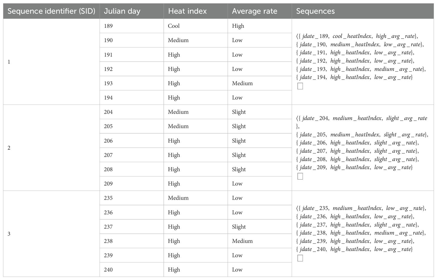
Table 1. Sample of sequences for cow ID 105 in Trial 1 during period $P_1$.

3.1.2 Definition 2 (horizontal sequence database)

The sequence database in this study is a collection of all information about daily heat index and behavior during the experiment. More formally, the definition of database is as follows:

A sequence database SDB is a list of sequences SDB = <s₁,s₂,.,s_p> having sequence identifiers (SIDs) 1,2,…,p.

Table 1 presents a portion of the sequence database SDB, containing three sequences for cow ID 105 in Trial 1 of our experiment. In this work, we use $s\in SDB$ to denote that s belongs to SDB.

3.1.3 Definition 3 (subsequence)

A subsequence is a smaller part of a sequence. More formally, the definition of a subsequence is defined as follows:

A sequence s_a = <A₁, A₂, … ,A_n> is said to be contained in a sequence s_b = <B₁, B₂, … ,B_m> if and only if there exist integers 1 ≤ j₁ < j₂ < ··· < j_n ≤ m such that $A_1\subseteq B_{j_1}$, $A_2\subseteq B_{j_2},\text{...},A_n\subseteq B_{j_n}$ (denoted as $s_a⊑s_b$).

For example, sequence s_a = <{high_heatIndex},{low_avg_rate}> is a subsequence of s_b = <{high_heatIndex},{high_heatIndex},{high_heatIndex, low_avg_rate}> because the first item in s_a is shown in s_b, the second itemset in s_a is subset of the third itemset of s_b.

3.14 Definition 4 (support)

The support of a sequence refers to the frequency or occurrence of a particular sequence within a database. It is a measure that helps to identify how commonly a sequence appears across all sequences in the database. More formally, the definition of support follows:

The support of a sequence s_a in a sequence database SDB is defined as the number of sequences $s\in SDB$ such that $s_a⊑s$ and is denoted by $su{p}_{SDB}(s_a)$.

In other word, $su{p}_{SDB}(s_a)=\left|\left\{s\right|s_a⊑s\wedge s\in SDB\}\right|$.

For example, consider the sequence s_a as follows:

$$s_a=\langle \left\{high\_heatIndex\right\}, \left\{high\_heatIndex\right\}, \left\{high\_heatIndex,low\_avg\_rate\right\}\rangle$$

Sequence s_a is the subsequence of sequences SID = 1, SID = 2 and SID = 3 in Table 1; thus, $su{p}_{SDB}(s_a)=3$.

3.1.5 Definition 5 (frequent sequential pattern discovery)

To ensure that only the most frequent sequences are considered, a minimum support threshold, minsup, is used to define them. A frequent sequential pattern is a sequence such that its support is greater than or equal to minsup. In other words, the goal is to identify the frequent subsequences that occur across many different sequences in the database. More formally, the definition of frequent sequential pattern is as follows:

Let minsup be a threshold provided by the user and SDB be a sequence database. A sequence s is a frequent sequential pattern if $su{p}_{SDB}(s)\ge minsup$.

3.2 Data preprocessing

3.2.1 Weather data

The raw weather 5-minute data containing air temperature and relative humidity were averaged hourly. Hourly Heat Index (HI) was computed using the following equations from the United States National Weather Service (https://www.wpc.ncep.noaa.gov/html/heatindex_equation.shtml), where T represents the hourly average air temperature in degrees Fahrenheit and RH represents the hourly average relative humidity:

$\begin{array}{ll}0.5 * \left\{T + 61.0 + [(T-68.0)*1.2] + (RH*0.094)\right\}& (1)\end{array}$

Then, the HI is equal to the average of the result from Equation 1 and air temperature. If HI exceeded 80 F, the following equation is applied.

If HI > 80, the regression equation of Rothfusz in 1990 is used, as shown below:

$\begin{array}{ll}HI= -42.379 + 2.04901523*T + 10.14333127*RH - 0.22475541*T*RH - 0.00683783*T^2 - 0.05481717*R{H}^2+ 0.00122874*T^2*RH + 0.00085282*T*R{H}^2 - 0.00000199*T^2*R{H}^2& (2)\end{array}$

If $RH<13\% and (T > 80 and T < 112)$, then the following is subtracted from Equation 2:

$$\frac{13-RH}{4}\times \sqrt{\frac{17-ABS(T-95)}{17}}$$

If $RH > 85\% and (T > 80 and T < 87)$, then the following is added to Equation 2:

$$\frac{RH-85}{10}\times \frac{87-T}{5}$$

The HI was then converted to Celsius for this paper. The equation to convert from Fahrenheit (°F) to Celsius (°C) is as follows:

$$\text{°C}=(\text{°F}-32)\times \frac{5}{9}$$

3.2.2 Behavior data and periods

We utilized three different metrics to define animal behavior, movement rate, activity and distance travelled from water. These metrics were calculated from the tracking data. Rate was calculated by dividing the spatial distance between successive positions by the temporal interval between the successive positions. Rate measures were then averaged hourly. Distance to water was the Euclidean distance between a position and the pasture’s only water source using the extract feature of ArcMap (https://www.esri.com/en-us/arcgis/products/arcgis-desktop/resources). Distances were averaged hourly. Activity was calculated using rate and criteria described by Augustine and Derner (2013) and Nyamuryekung’e et al. (2020). Cattle activity can have value 0 and 1. Cattle were considered inactive when rate was less than 2.34 m/min for each position. A value of 0 was assigned for activity when rate was less than 2.34 m/min, and a value of 1 for activity when rate was greater than 2.34 m/min. If there were less than 3 positions recorded during an hour (poor GPS performance), the hourly average activity was not calculated and not used. If there were 3 or more positions per hour, activities were averaged each hour.

Using all the rate and activity data in Trial 1, we selected two periods to define typical grazing and grazing periods (Figure 1). Period P₁ is from 5:00 AM to 8:00 AM and 5:00 PM to 8:00 PM, which focuses on the two major grazing bouts of cattle on rangeland (Kilgour et al., 2012). Period P₂ is from 5:00 AM to 8:00 PM, which cover all activities during the day, when activity and movement are usually higher compared to night.

Figure 1

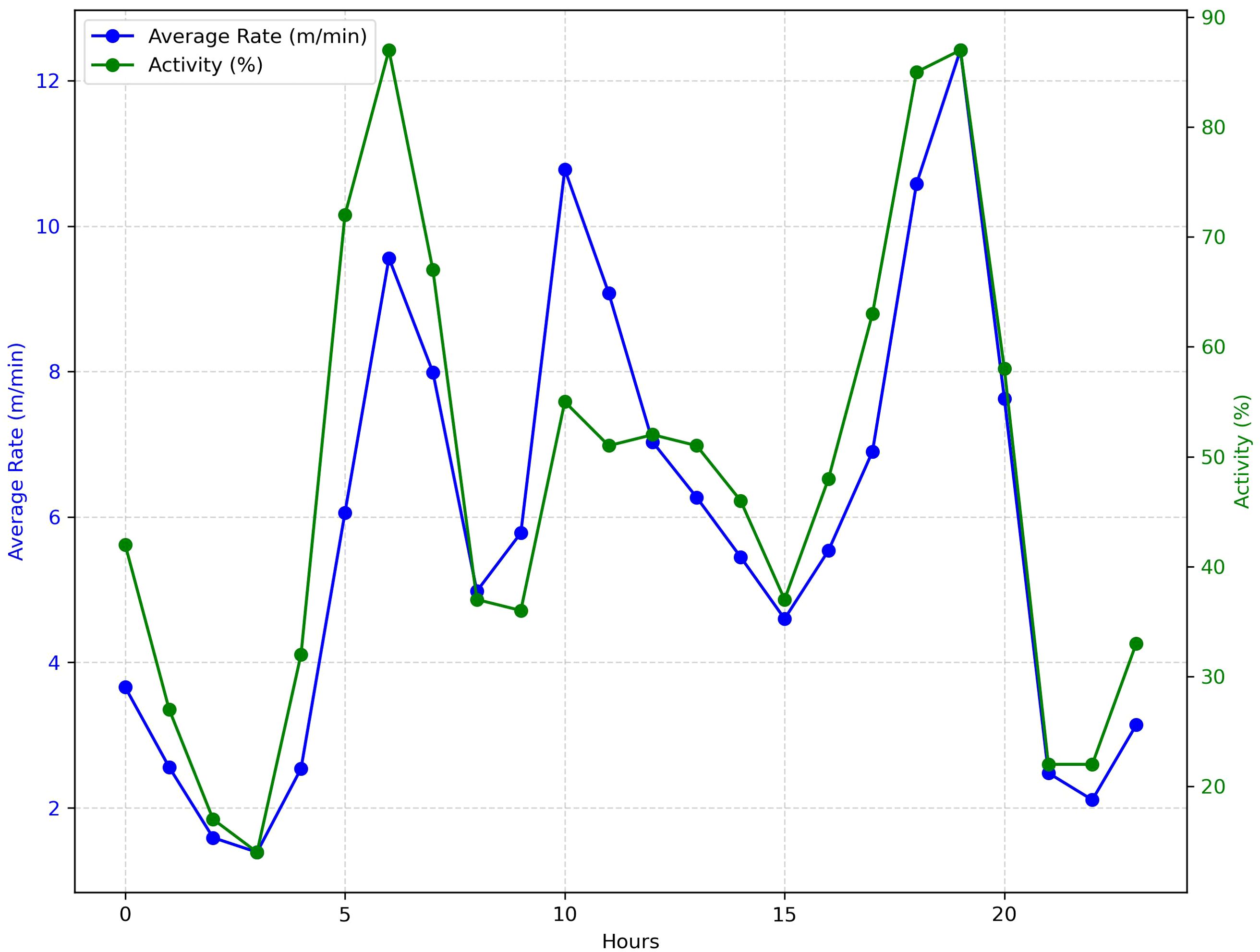
Figure 1. The average movement rate and the percentage of activity by hour for all animals during Trial 1, showing two common peaks in the morning and evening grazing bouts.

These variables were selected because they may be useful for monitoring common behaviors cattle show during periods of heat stress (reduced feed intake, increased water intake and decreased activity) (Alves et al., 2020). Changes in movement rate during the primary grazing bouts may reflect changes in forage intake. Decreased distance travelled from water may reflect increased visits to water and more time spent near water, which may occur in response to increased water intake. Our activity measure should reflect changes in cattle activity.

3.2.3 Database for sequence pattern mining

Hourly averages of movement rate, activity, and distance travelled from water were averaged within each period (P₁ and P₂) for the data mining analysis. The other hourly averages were not used in data mining. For each day, the HI and behavior metrics were categorized into three (cool, medium and high) and four levels (low, slight, medium, and high), respectively, using k-means clustering method outlined in Section 3.3.1. Experimental data were then segmented into six-day intervals, with a sliding window of one day. For example, Figure 2 illustrates two segments in which the first segment contains data from Julian dates 156 (June 5^th, 2019) to 161 (June 10^th, 2019) and the second segment contains data from Julian dates 157 (June 6^th, 2019) to 162 (June 11^th, 2019). For the purpose of applying algorithm, Julian dates are used instead of dates in the day, month and year format. When using movement rate (representing cattle behavior) and HI, the set of items (Definition 1) is I = {jdate_156, jdate_157,…, jdate_259, jdate_260, cool_heatIndex, medium_heatIndex, high_heatIndex, low_avg_rate, slight_avg_rate, medium_avg_rate, high_avg_rate}. An itemset consisting of three items: a Julian date encoded as jdate_index, where $index\in \left\{156,157,\dots ,260\right\}$; the HI level encoded as low_heatIndex, medium_heatIndex, and high_heatIndex; and the movement rate level encoded as low_avg_rate, slight_avg_rate, medium_avg_rate, and high_avg_rate. Formally, based on Definition 1, the sequence formed from weather and movement rate data is an ordered list of information spanning six continuous days (n = 6). Each day’s information is represented as an itemset. The sequence database, which treats movement rate as behavior, includes all sequences with movement rate levels. In the same way, the sequence databases using activity and distance travelled from water as behavior metric are constructed using activity levels and distance travelled from water levels, respectively.

Figure 2

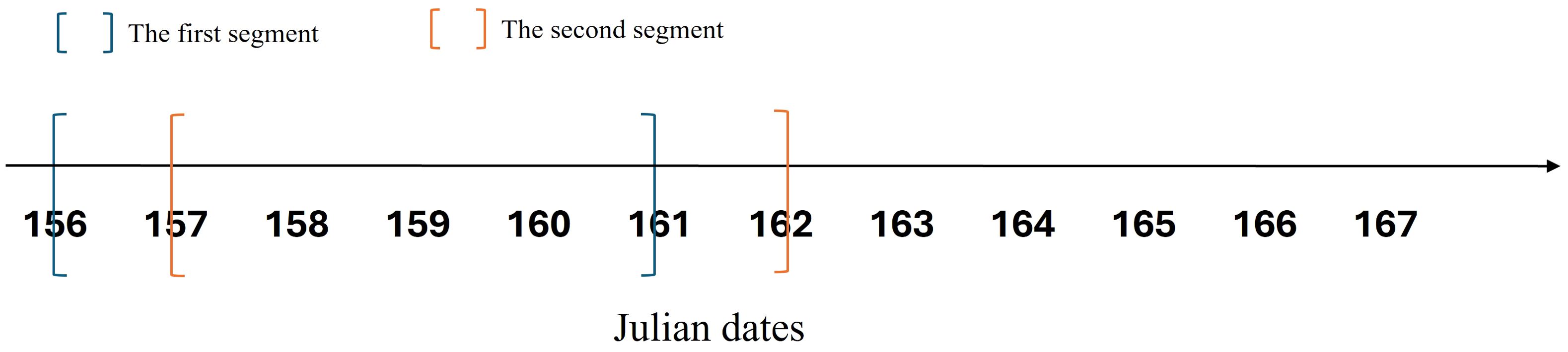
Figure 2. Segmentation of data into six-day intervals with a sliding window one day. The first and second segments contain weather and behavior data from Julian dates from 156 to 161 and 157 to 162, respectively.

3.3 Data mining approach

Given the availability of both weather and GPS datasets, the weather data was first processed using the method described in Section 3.2.1 to compute the HI. The GPS data was then used to calculate three behavioral metrics: movement rate, activity level, and distance traveled from water—each representing cattle behavior in Section 3.2.2.

In this section, the clustering method described in Section 3.3.1 is applied separately to the HI dataset and to each of the three behavioral datasets. As a result, for each individual cattle and each day, an HI level and a corresponding behavioral level are assigned. This process generates separate databases for each behavioral metric, which are then used for sequence pattern mining, described in Section 3.2.3.

Subsequently, the CM-SPAM algorithm from the SPMF data mining library in Section 3.3.2 is applied to each cattle’s behavioral database to extract frequent sequential patterns, revealing relationships between heat stress and reductions in behavior.

Finally, Section 3.3.3 details the analysis of detected continuous patterns by comparing behavior during hot weather with behavior observed during the preceding cool weather day.

3.3.1 Clustering for weather data and behavior data

To categorize the weather for each day, we applied K-means clustering method (Tan et al., 2016). This is an unsupervised learning technique that partitions the data into k groups based on their distance from centroids. Given k, the process is described as follows:

● Step 1: Randomly select k centroids and partition the data points into k non-empty non-overlapping subsets.

● Step 2: Calculate the centroids of the clusters from the current partition, with each centroid representing the mean of its the mean point of the cluster.

● Step 3: Assign each data point to the cluster with the nearest centroid.

● Step 4: If no new assignment occurs, the algorithm stops. Otherwise, go to step 2.

In our experiment, we set k = 3 to represent three weather levels, hot, medium and cool. In addition, to handle sudden weather changes such as storms that lead to a very low value of HI, we utilized k-means clustering method with constraint, ensuring each cluster contains at least five data points (Bradley et al., 2000). The cluster size constraint is met by formulating the assignment step 3 as a Minimum Cost Flow (MCF) problem (Bertsekas, 1991) and the MCF algorithm is used to ensure that each cluster receives the required minimum number of points. This constraint prevents the creation of a cluster solely based on the extreme low HI values, ensuring that the cluster representing cool weather is more representative of typical cool weather conditions, rather than being influenced by anomalous values.

In the same way, to categorize the cattle behavior, movement rate, activity and distance travelled from water, into four levels: high, medium, slight or low, we utilized the k-means clustering method to divide the daily average of each behavior metric into four distinct clusters. For this analysis, we set k = 4 and included the constraint that each group must have at least five data points.

3.3.2 CM-SPAM algorithm

Mining frequent sequential patterns is a challenging and computationally expensive task due to the exponential growth in the number of subsequences. For example, considering a sequence containing q items, it can have up to 2^q-1 distinct subsequences, all of which could potentially be candidates for frequent sequential patterns (Fournier-Viger et al., 2017). Alternatively, when considering the total number of k-sequences (sequences contains k items) present in n itemsets is $(\frac{n}{k})$ (Tan et al., 2016). In this study, we apply an unsupervised Co-occurrence Map Sequential Pattern Mining (CM-SPAM) algorithm (Fournier-Viger et al., 2014) for discovering all frequent sequential patterns. It is one of the most advantageous techniques and has been applied in various fields, such as discovering frequent nucleotide patterns related to COVID 19 (Nawaz et al., 2021) and identifying frequent API call patterns in malware behavior analysis (Nawaz et al., 2022; Pektaş, 2018).

CM-SPAM is a sequential pattern mining algorithm built on the SPAM algorithm (Ayres et al., 2002). It utilizes a depth-first search algorithm to discover patterns through the following steps:

● Step 1: First, the database is scanned to identify sequences containing single items such as <{high_heatIndex}>, <{low_avg_rate}>, and <{medium_avg_rate}>. The frequent single-item sequences, whose support is higher than a given threshold, are referred to as 1-sequences.

● Step 2: The algorithm recursively performs two operations, s-extensions and i-extensions, to generate larger subsequences as follows:

○ Order of items: To begin the extension process, it assumes that all items are ordered in either decreasing or increasing lexicographical order (denoted as $\succ$) such as $medium\_avg\_rate\succ low\_avg\_rate\succ high\_heatIndex.$ Note that the specific order does not affect the final result, but is used to explore the potential sequential patterns and avoid considering the same pattern multiple times.

○ s-extensions: Given a sequence $s_a=I_1,I_2,\dots ,I_n$ and an item x, an s-extension of sequence s_a is formed as $s_b=I_1,I_2,\dots ,I_h,\left\{x\right\}$;

○ i-extensions: Given a sequence $s_a=I_1,I_2,\dots ,I_n$ and an item x, an i-extension of sequence s_a is formed as $s_b=I_1,I_2,\dots ,I_h\cup \left\{x\right\}$ such that x is the last item in I_h according to the lexicographical order $\succ$.

For example, given a sequence $s_a=\langle \left\{high\_heatIndex\right\}\rangle$ with item low_avg_rate, an s-extension is $\langle \left\{high\_heatIndex\right\},\left\{low\_avg\_rate\right\}\rangle$ and an i-extension is $\langle \left\{high\_heatIndex,low\_avg\_rate\right\}\rangle$.

Using the s-extensions and i-extensions, the algorithm generates (k+1)-sequences from one or more frequent k-sequence. If a sequence can no longer be extended, the algorithm backtracks and continues generating other patterns using another sequence.

In this study, the SPMF data mining library (https://www.philippe-fournier-viger.com/spmf/), an open-source Java library, is utilized to call the CM-SPAM algorithm (Fournier-Viger et al., 2017). Four parameters are configured. First, minimum support threshold (minsup) is determined. If minsup threshold is too low, it may result in an overwhelming number of patterns, which may slow down the algorithm. Conversely, if minsup threshold is set too high, too few patterns may be identified. In this work, conducted over two different periods P₁ and P₂, because the length of period P₁ is shorter than P₂, the setup of minsup is 20% for period P₁ and 25% for period P₂ It means that a pattern is considered frequent in P₁, it must appear in at least 20% of sequences in the dataset from P₁, and a pattern is considered frequent in P₂, it must appear in at least 25% of sequences in the dataset from P₂. The value of minsup varies among different problems; however, these values should not be too low, because they have been used in discovering sequential pattern mining in COVID-19 genome using CM-SPAM (Nawaz et al., 2021). Second, the minimum number of items required in a pattern is set to three in this study. This is because we aim to identify continuous patterns spanning at least two days, which includes the weather level on the first day and both the weather and behavior levels on the second day. The third parameter is required items, which ensure the detection of a decrease in animal behavior. Required items that the frequent pattern must contain are low level values of each metric (e.g. low_avg_rate). Finally, the max gap parameter specifies whether gaps between item sets (meaning day’s information) are allowed in sequential patterns. We have set it to be one to prevent any gap between item sets, meaning that the frequent sequential pattern identified in our experiment corresponds to continuous days.

3.3.3 Examining the continuous patterns

To investigate the influence of continuous patterns on animal behavior in comparison to cool days, we calculated three values: (1) the frequency of decrease in the behavior metric between the closest cool weather day d before a pattern s begins and the last day d_last of that pattern, (2) the average decrease in the behavior metric from d and d_last​ across patterns, and (3) the average difference in the behavior metric between d and d_last​ for each pattern. Because the hot weather can last for several days (Trial 1), day d is defined as either: (1) the closest cool day—the nearest day within the week before the pattern start day on which the cool-level HI occurred; or (2) the closest medium weather day—the nearest day before the pattern start day on which the medium-level HI occurred.

Let CP be the set of continuous patterns found in data of a cow, and |CP| be the number of patterns in CP. Let $B_d^s$ and $B_{d_{last}}^s$ represent the behavior metrics on day d and d_last related to continuous pattern $s\in CP$ (as defined above). Let C be the set of patterns $s\in CP$ such that $B_d^s>B_{d_{last}}^s$, and let |C| be the number of patterns in C.

The frequency of decrease in the behavior metric for a cow is defined as follows:

$$\frac{\left|C\right|}{\left|CP\right|}$$

The average decrease in the behavior metric between days d and d_last for a cow is defined as follows:

$\begin{array}{ll}\frac{{\sum }_{s\in C}(B_d^s-B_{d_{last}}^s)}{\left|C\right|}& (3)\end{array}$

The average difference in the behavior metric between days d and d_last for a cow is defined as follows:

$\begin{array}{ll}\frac{{\sum }_{s\in CP}(B_d^s-B_{d_{last}}^s)}{\left|CP\right|}& (4)\end{array}$

The difference between Equation 3 and Equation 4 is that Equation 3 calculates the average decrease when the behavior metric on day d_last is lower than that on day d, whereas Equation 4 computes the overall difference in behavior metric between days d and d_last.

In this study, this exploration was applied to the behavior metric (rate, m/min) that most successfully detects the continuous pattern.

3.3.4 Binomial probability

To determine whether the detected patterns are unlikely due to chance, we apply binomial probability to Trial 1 and Trial 2. The binomial probability is calculated using the following equation:

$$P(X=k)=\frac{n!}{(n-k)!k!}{p}^k{(1-p)}^{n-k}$$

where:

n: total number of m continuous hot days across all animals.

k: total occurrences of the m-day continuous pattern detected across all animals in our study.

p = 0.25: The probability of an m-day continuous pattern, based on the assumption that on a last day of a pattern, the animal behavior is equally likely to be one of four levels (low, slight, medium, high), and the animal behavior is associated with “low” movement rate on the day.

In this study, we analyze the most successfully detected frequent continuous patterns for Trial 1 and Trial 2.

4 Results

4.1 K-means weather clusters for trials 1 and 2

Based on the cluster method, the temperature of hot weather periods in Trial 1 was greater than or equal to 30°C (Figure 3). The medium weather period varied between 27°C to 30°C. The cool weather was below 27°C. Two notable temperature drops occur on Julian dates 212 and 225 (Figure 3).

Figure 3

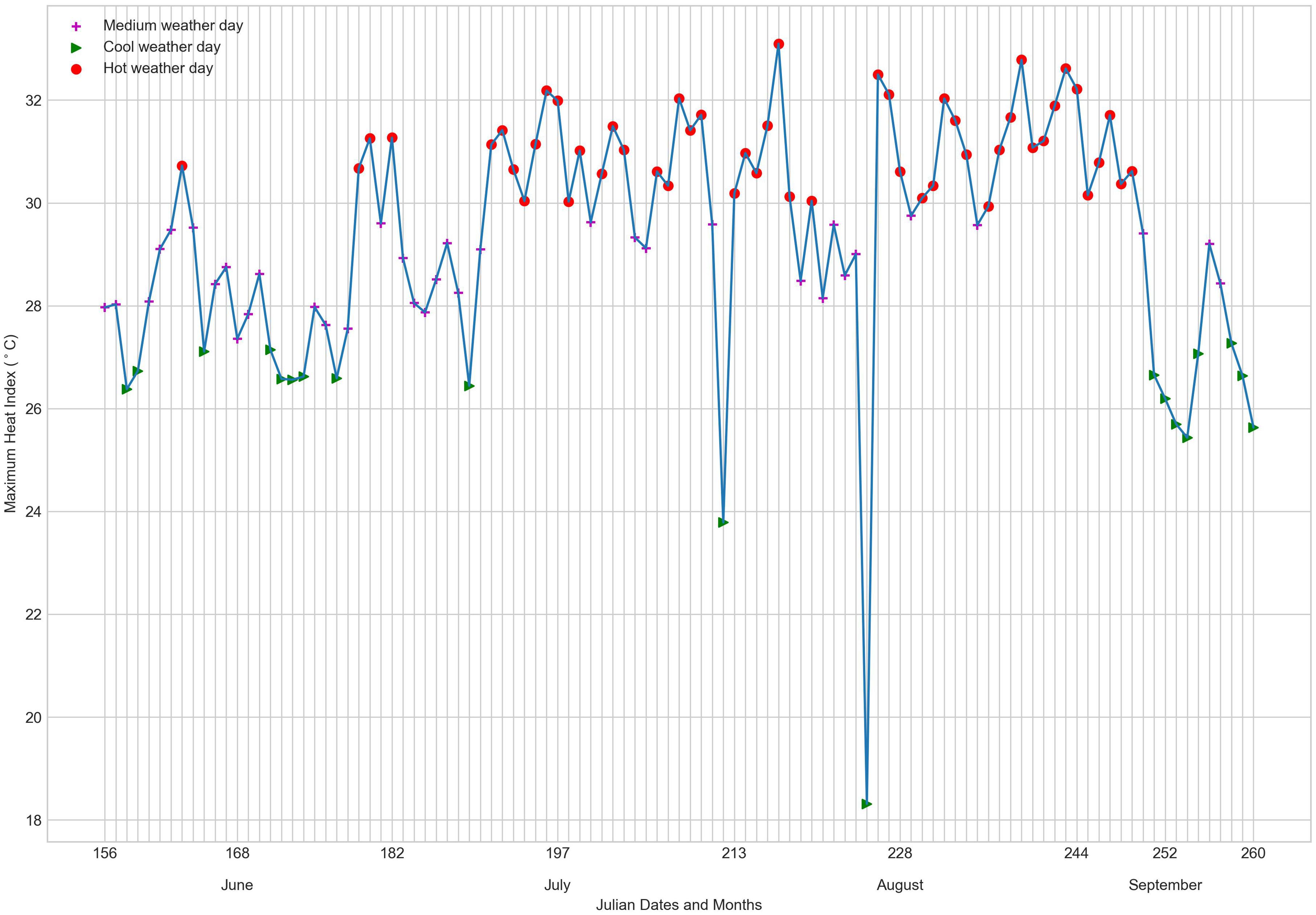
Figure 3. Three weather levels (hot, medium, and cool weather days) calculated using the K-means clustering method with the constraint across days in Trial 1.

In Trial 2, the weather threshold calculated from the cluster method was slightly lower than in Trial 1. The hot weather is defined as 29.5°C or higher (Figure 4). The medium weather ranges from 26°C to 29.5°C. The cool weather was below 26°C.

Figure 4

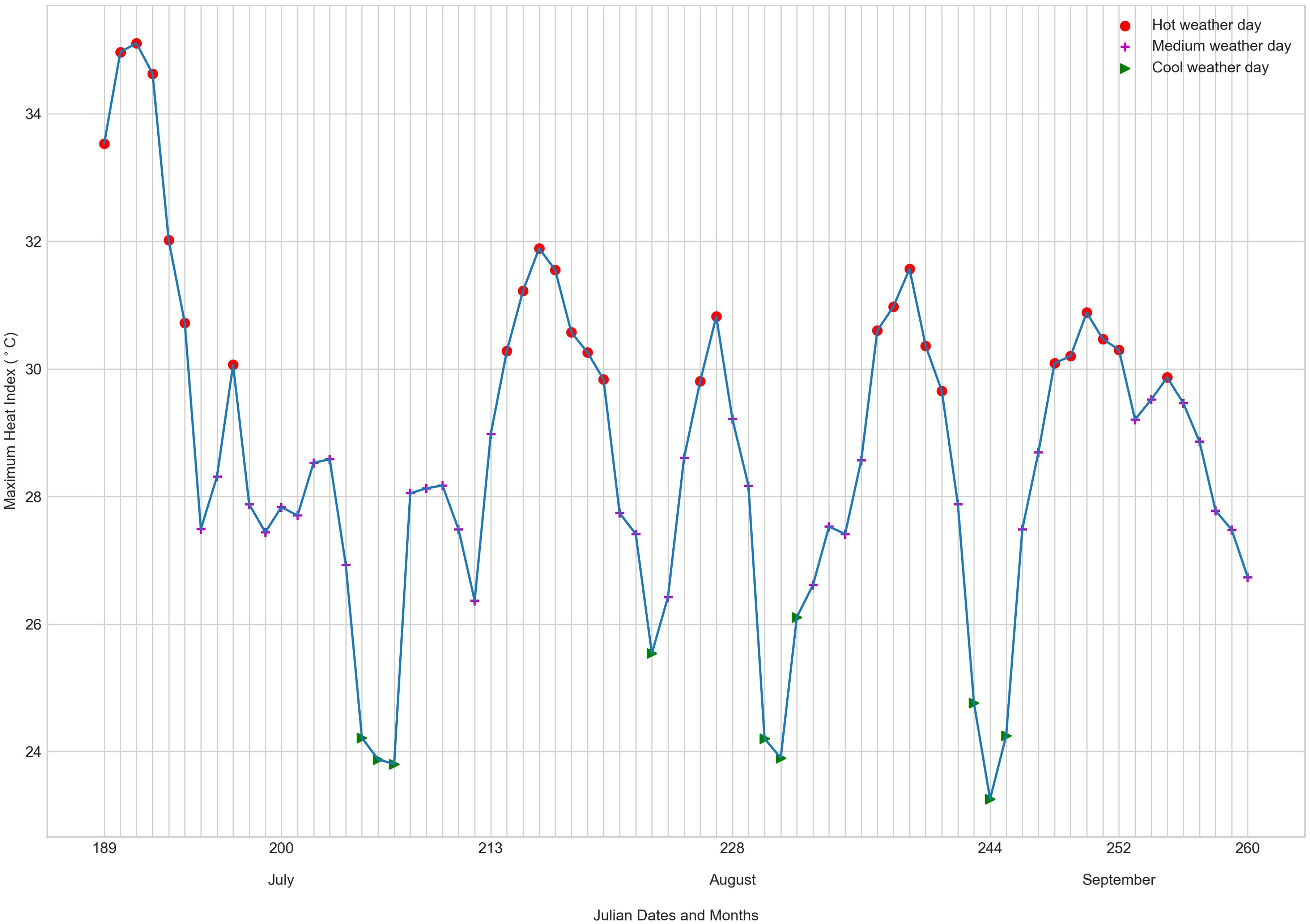
Figure 4. Three weather levels (hot, medium, and cool weather days) calculated using the K-means clustering method with the constraint across days in Trial 2.

4.2 CM-SPAM algorithm for pattern recognition of behavior and weather data for Trial 1

The following describes different continuous patterns that were identified and detected in this work.

● A four-day continuous pattern with regard to a behavior metric A is described as: “The first day features a high HI, the second day also has a high HI, the third day continues with a high HI, and the fourth day shows a low average of A along with a high HI”.

● A three-day continuous pattern with regard to a behavior metric A is described as: “The first day has a high HI, the second day also has a high HI, and the third day presents a low average of A alongside a high HI”.

● A two-day continuous pattern with regard to a behavior metric A is described as: “The first day experiences a high HI, and the second day shows a low average of A with a high HI”.

During period P₁ (5:00 AM to 8:00 AM and 5:00 PM to 8:00 PM), by utilizing average daily rate, CM-SPAM successfully identifies the pattern between hot weather and low movement rate, with 90.91% of animals exhibiting the three-day continuous pattern. Among these, 54.55% animals show four-day continuous patterns (Figures 5–8). Only two animals (9.09%) do not display any four-day or three-day continuous patterns. In contrast, when the algorithm analyses the average daily activity metric, which is another cattle behavior metric, it fails to detect relationship between hot weather and low average daily activity. The majority of animals (95.45%) show no four-day or three-day continuous patterns related to hot weather and low in activity. Only one animal demonstrates the three-day continuous pattern (Figure 9). When CM-SPAM is applied to average daily distance to water (the third cattle behavior metric), only one animal showed four-day continuous pattern. More cows (31.82%) displayed a three-day continuous pattern, while 68.18% of cows did not show any four-day or three-day continuous patterns linked to hot weather and low in distance to water (Figure 10) (Table 2).

Figure 5

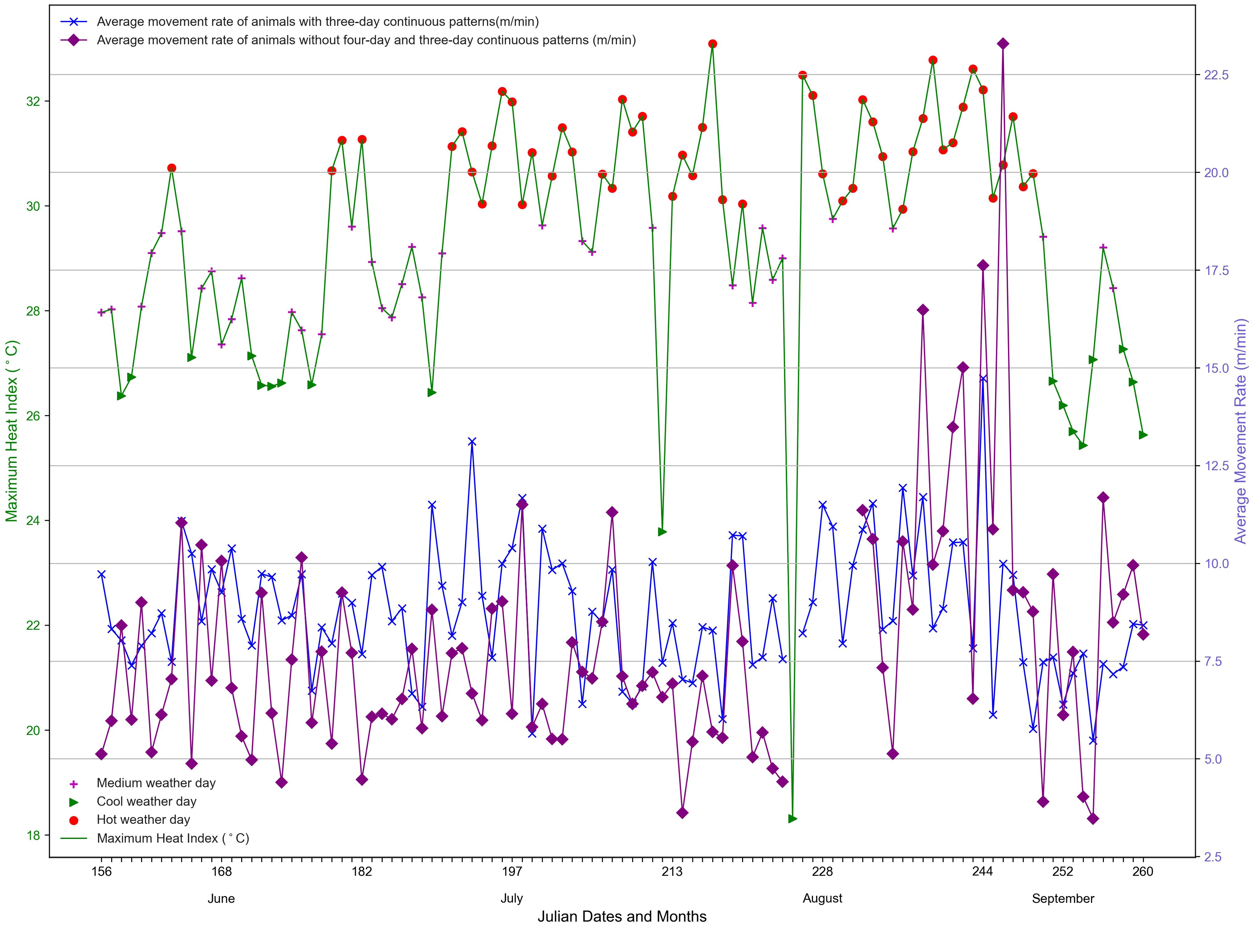
Figure 5. Average movement rate of cows with three-day continuous patterns and the average rate of cows without continuous patterns (three-day and four-day) in period $P_1$ of Trial 1. Daily maximum heat index helps identify periods of hot weather.

Figure 6

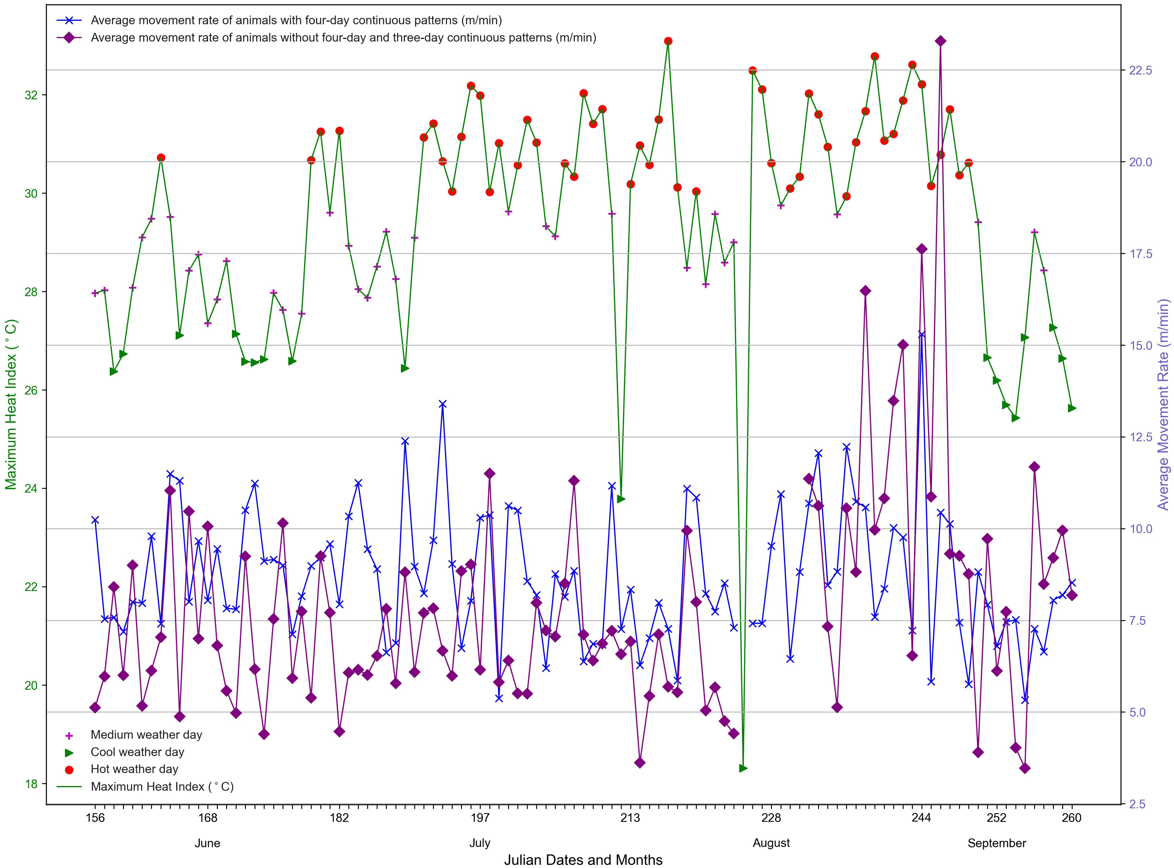
Figure 6. Average movement rate of cows with four-day continuous patterns and the average rate of cows without continuous patterns (both three-day and four-day) in period $P_1$ of Trial 1. Daily maximum heat index helps identify periods of hot weather.

Figure 7

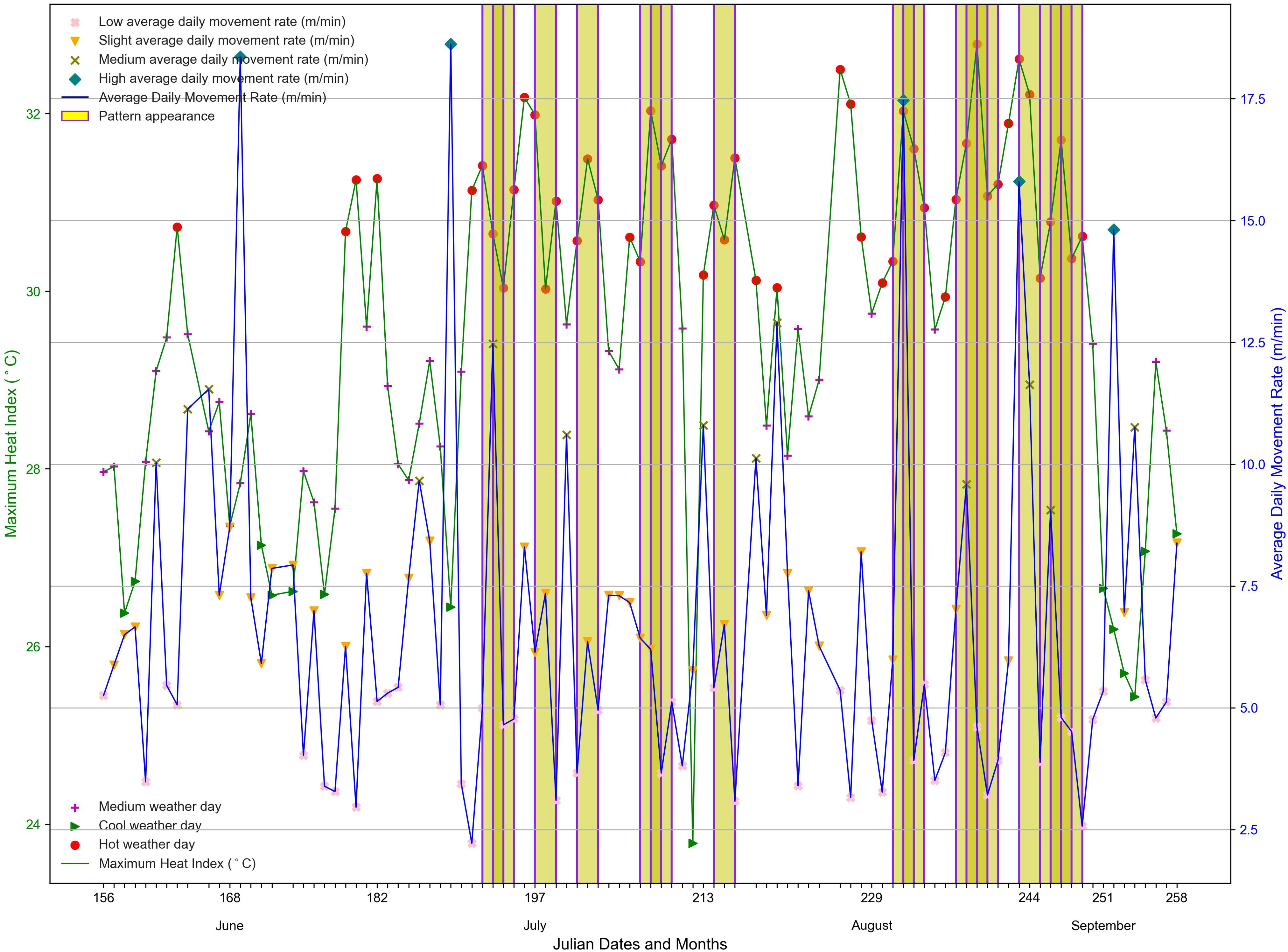
Figure 7. Three-day continuous patterns using the movement rate metric for cow 105 in Trial 1 during period $P_1$, with detected patterns highlighted.

Figure 8

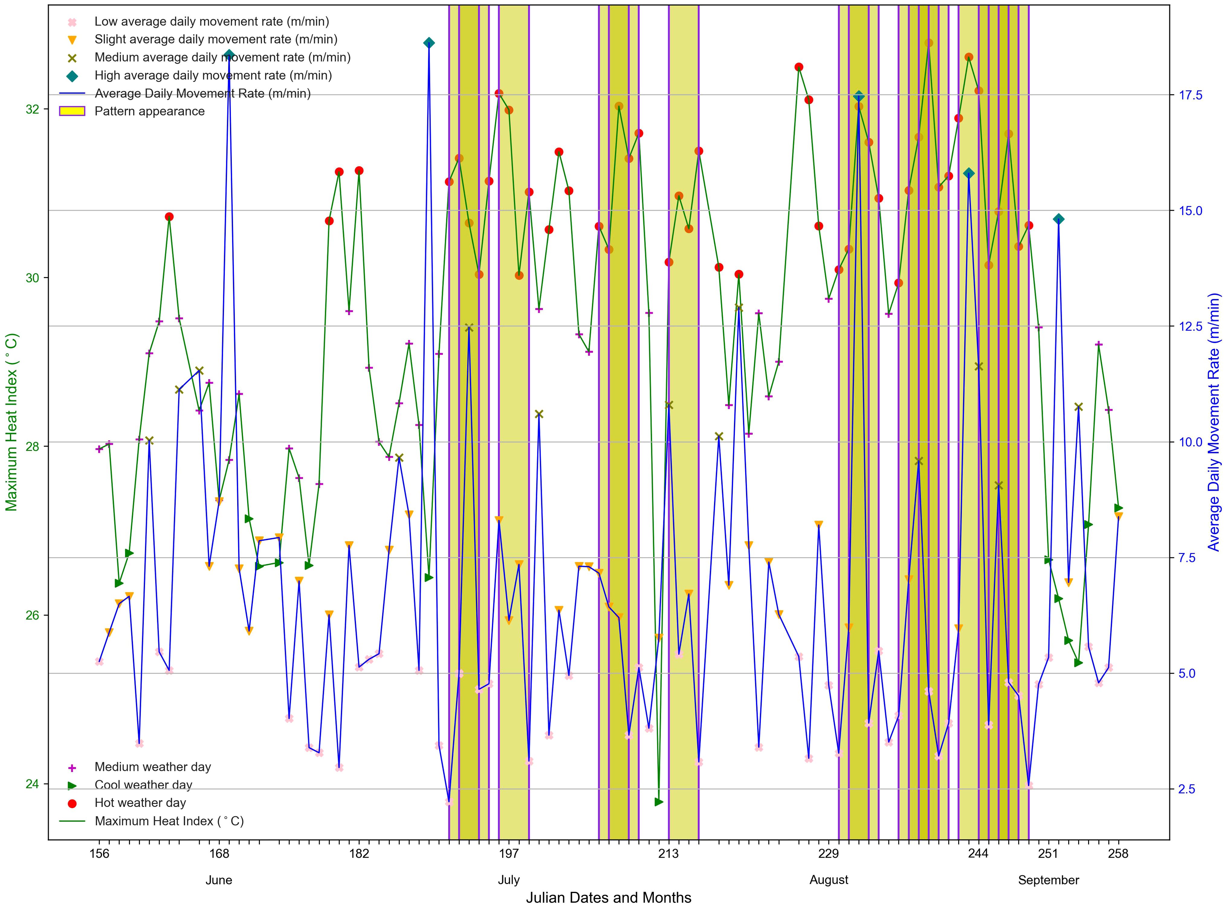
Figure 8. Four-day continuous patterns using movement rate metric for cow ID 105 in Trial 1 during period $P_1$, with detected patterns highlighted.

Figure 9

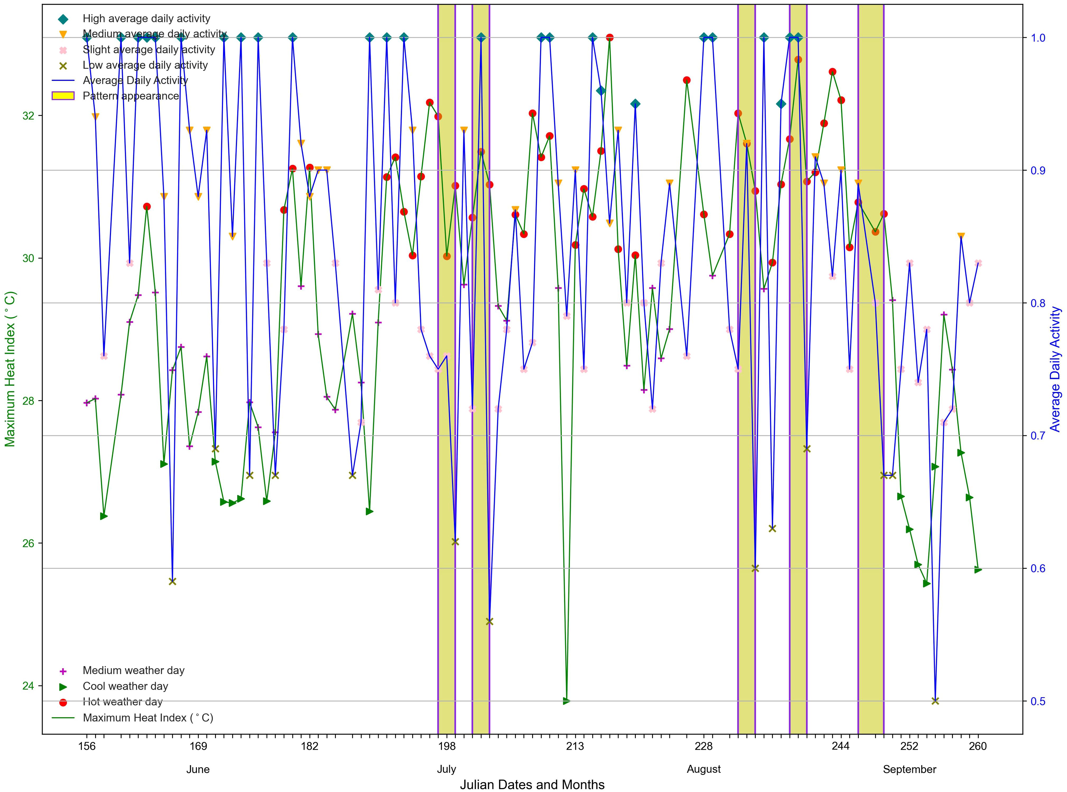
Figure 9. Three-day continuous patterns using activity metric for cow ID 704 in Trial 1 during period $P_1$, with detected patterns highlighted.

Figure 10

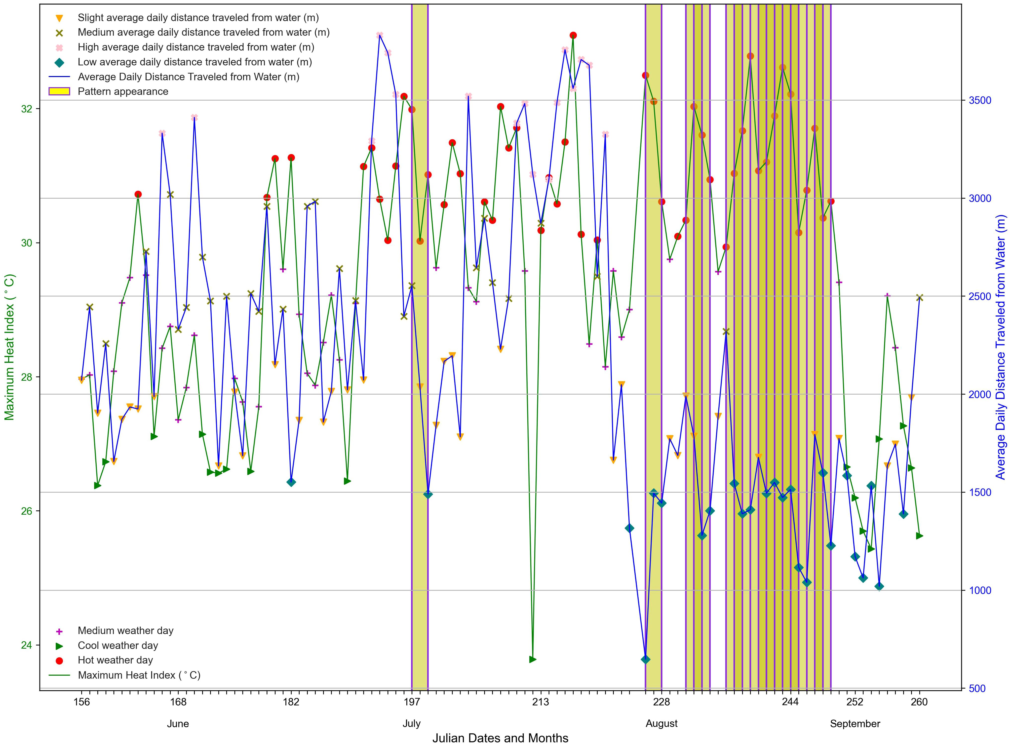
Figure 10. Three-day continuous pattern using distance traveled from water metric for cow ID 229 in Trial 1 during period $P_1$, with detected patterns highlighted.

Table 2

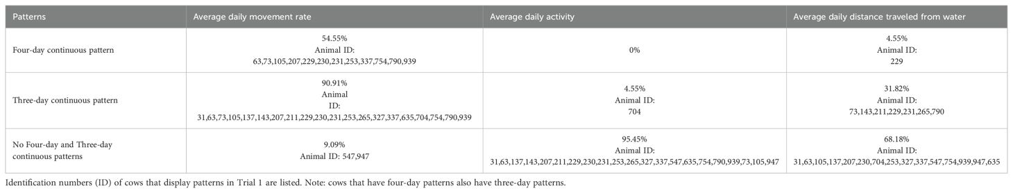
Table 2. Percentage of cows with patterns during period $P_1$ in Trial 1 for the behavioral metrics: average daily movement rate, average daily activity and average daily distance travelled from water.

In period P₂ (5:00 AM to 8:00 PM), 54.55% of the cows displayed three-day continuous patterns related to their average daily rate, with 13.64% of them showing four-day continuous pattern. Meanwhile, 45.45% of animals do not exhibit either four-day or three-day continuous pattern. When analysing daily average activity and average daily distance to water, the results are similar to those in the period P₁. The algorithm did not identify a connection between hot weather and a decrease in this behavior, and 95.45% of the cows did not show any three-day or four-day continuous patterns when considering average daily activity. For daily distance travelled to water, 31.82% of animals displayed three-day continuous patterns (Table 3).

Table 3

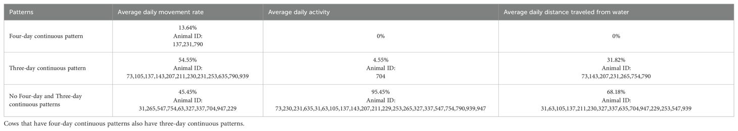
Table 3. Percentage of cows with patterns during period $P_2$ of Trial 1 using the behavioral metrics average daily movement rate, average daily activity and average daily distance travel from water. Identification numbers (ID) of cows displaying patterns are listed.

When the three-day continuous patterns were detected using movement rate during period P₁ for 20 cows out of 22 cows, the frequency of decreases in rate had minimum, maximum and mean values of 53%, 100% and 87%, respectively (Table 4). The average decrease in movement rate from the last cool day within a week before a three-day continuous pattern began or the last medium weather day to the last hot day in the pattern among 20 cows ranged from 2.17 (m/min) to 8.0 (m/min), with a mean of 4.57 (m/min). The minimum, maximum and mean values of average difference in rates during hot days and the previous cool day within a week or the closest medium weather day are 0.61 (m/min), 8.0 (m/min) and 3.93 (m/min), respectively. For the 12 cows exhibiting four-day continuous pattern in period P₁ using movement rate, the minimum frequency of decreases in rate was slightly higher than that of three-day continuous pattern (55%), with four cows showing 100% frequency of decrease and a mean frequency of 82%. The minimum, maximum and mean values of average decrease in movement rate from the previous cool day within a week before a four-day continuous pattern started or the last medium weather day to the end of the hot period in the pattern were slightly higher compared to the three-day continuous pattern, with values of 2.38 (m/min), 8.64 (m/min) and 5.43 (m/min), respectively. Similarly, the minimum, maximum and mean values for the average differences between the four-day continuous hot days and the cool day within a week or the closest medium weather day were slightly higher than those for three-day continuous pattern, with values of 1.26 (m/min), 8.37 (m/min) and 4.37 (m/min) (Table 4).

Table 4

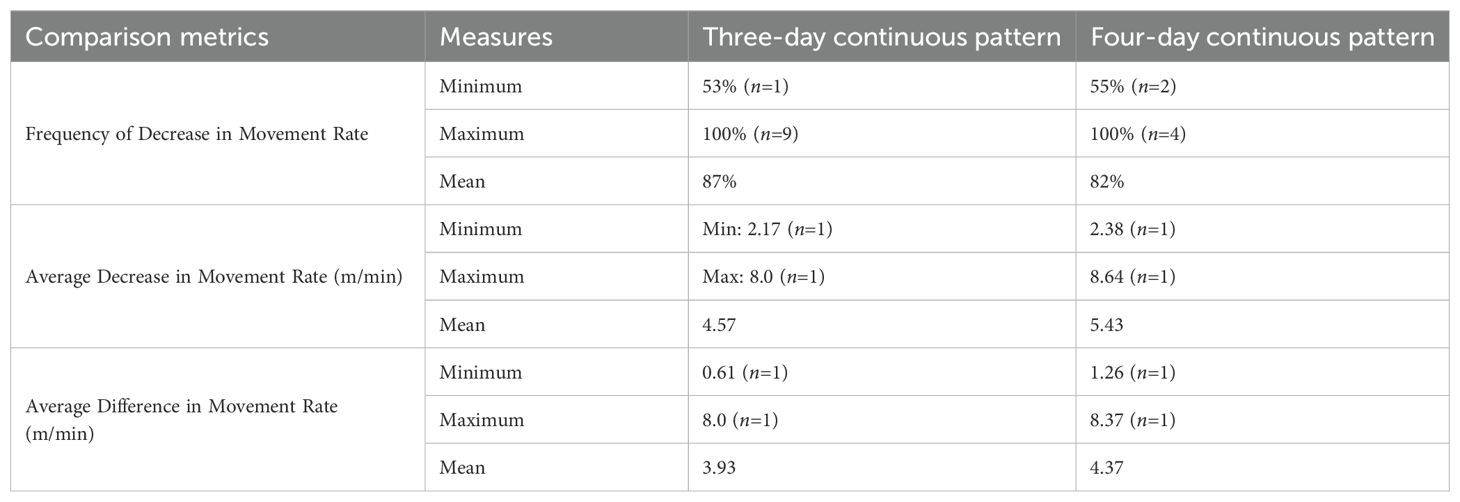
Table 4. Comparison of movement rate changes between the closest cool day within seven days or the closest medium weather day before the first day of the three-day (or four-day) continuous pattern and the third day (or fourth day) of the three-day (or four-day) continuous pattern during period $P_1$ in Trial 1, including minimum, maximum and mean values for the frequency of decreased movement rates, average of movement rate decrease (prior to until the end), and overall movement rate difference (prior to versus hot period) for animals with three-day (or four-day) continuous patterns, along with the number of animals $n$ having the minimum and maximum values.

The binomial probability was calculated during P₁ period, based on the movement rate behavior metric over the three-day continuous patterns. With m = 3, n = 622, k = 214, we find that $P(X=214)<0.0001$.

4.3 CM-SPAM algorithm for pattern recognition of behavior and weather data for trial 2

Because the frequency of hot weather in Trial 2 is lower than in Trial 1, and the duration of dataset in Trial 2 is shorter than in Trial 1 (less than one month), two-day continuous patterns are included in the results. In period P₁ (5:00 AM to 8:00 AM and 5:00 PM to 8:00 PM), utilizing average daily rate, CM-SPAM algorithm identified 71.43% of animals exhibited a two-day continuous pattern between hot weather and low in movement rate levels. Among these, 42.86% show three-day continuous pattern. Meanwhile, 28.57% of animals did not display any continuous patterns (two-day, three-day or four-day) related to hot weather and low movement rate (Figures 11–14). When considering average daily activity as a behavior metric, 28.57% of animals show a two-day continuous pattern, while the rest did not show any connection between hot weather and low activity (Figure 15). CM-SPAM is unable to detect any pattern linking hot weather and distance travelled to water, with 100% of animals showing no relationship (Table 5).

Figure 11

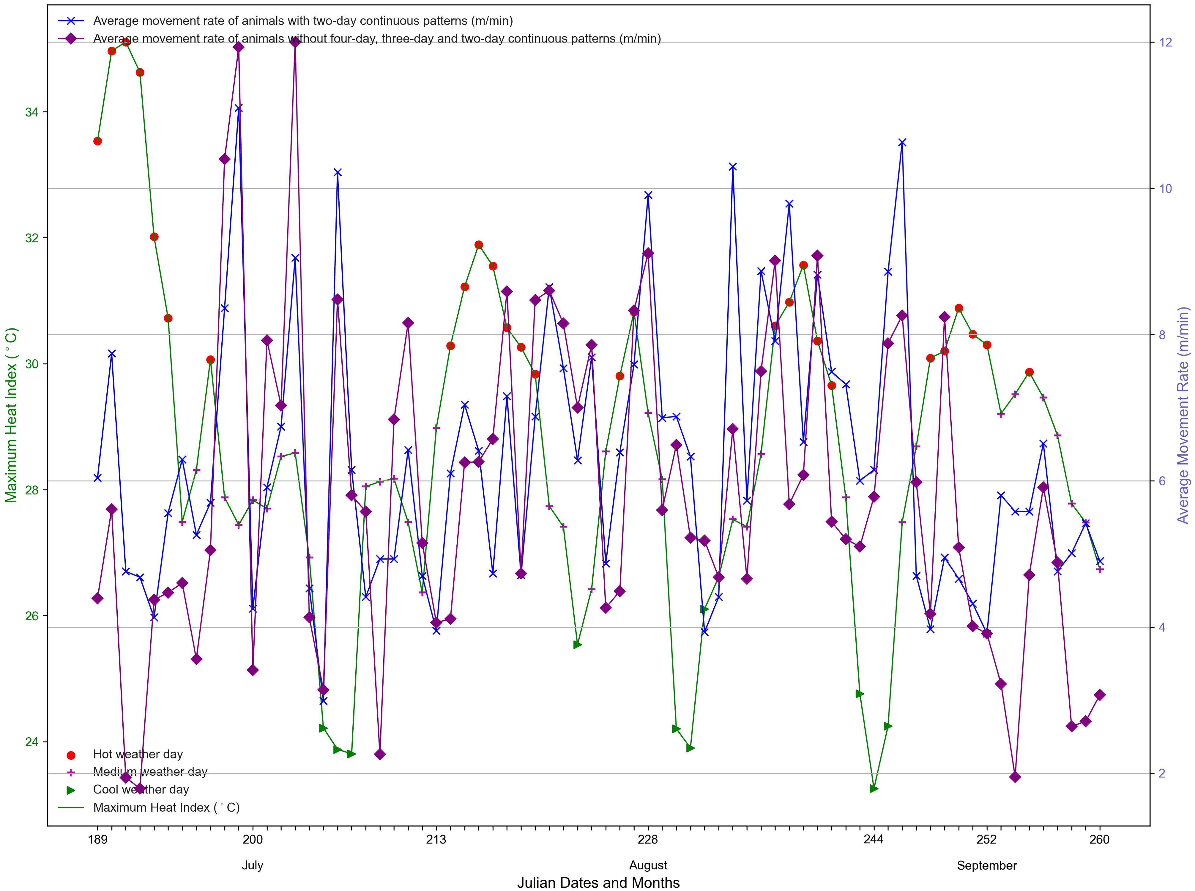
Figure 11. Average movement rates of cows with two-day continuous patterns and the average rates of cows without continuous patterns (two-day, three-day and four-day) in period $P_1$ of Trial 2. Daily maximum heat index helps identify hot periods.

Figure 12

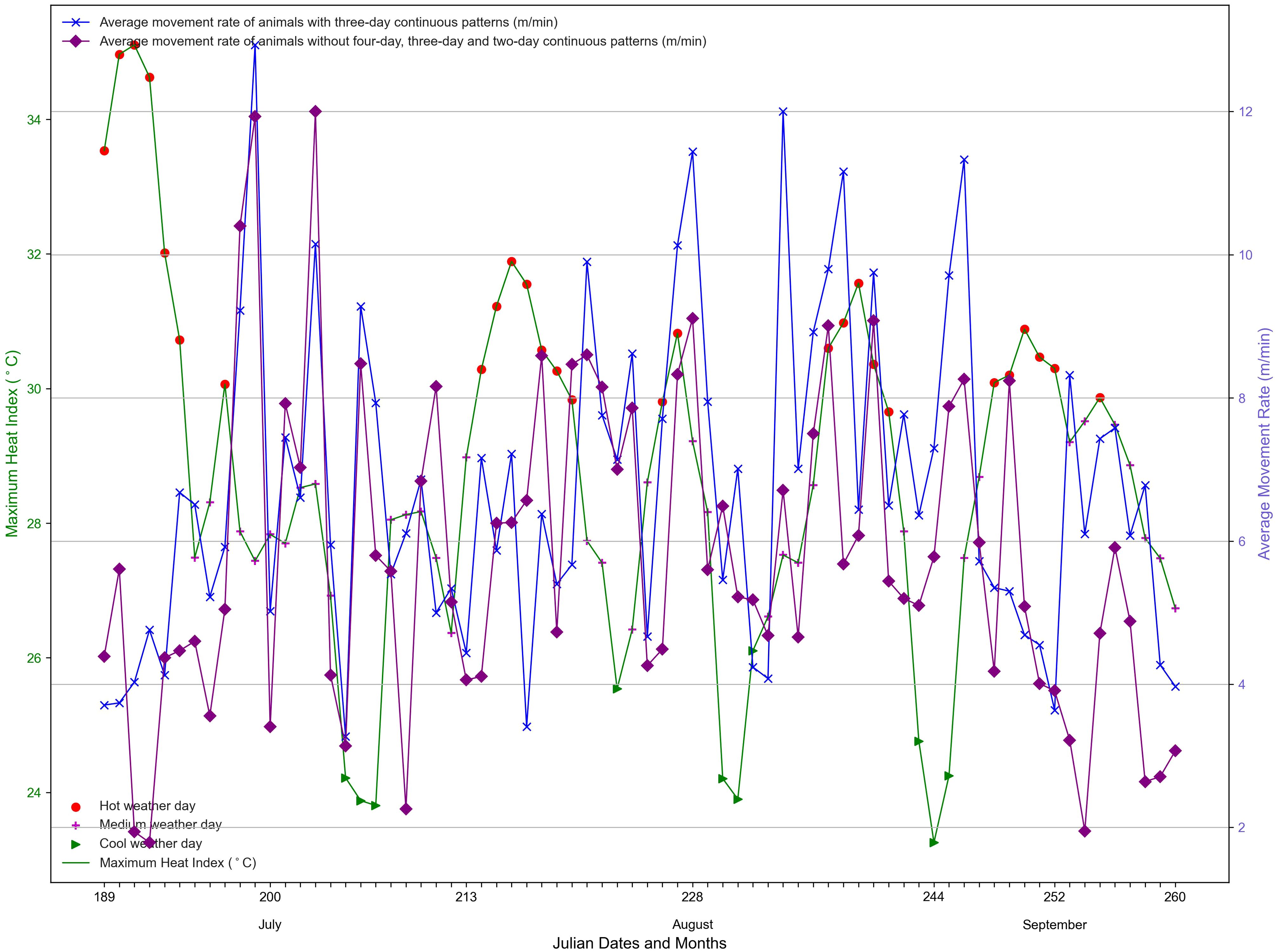
Figure 12. Average movement rates of cows with three-day continuous patterns and the average rates of cows without continuous patterns (two-day, three-day and four-day) in period $P_1$ of Trial 2. Daily maximum heat index helps identify periods of hot weather.

Figure 13

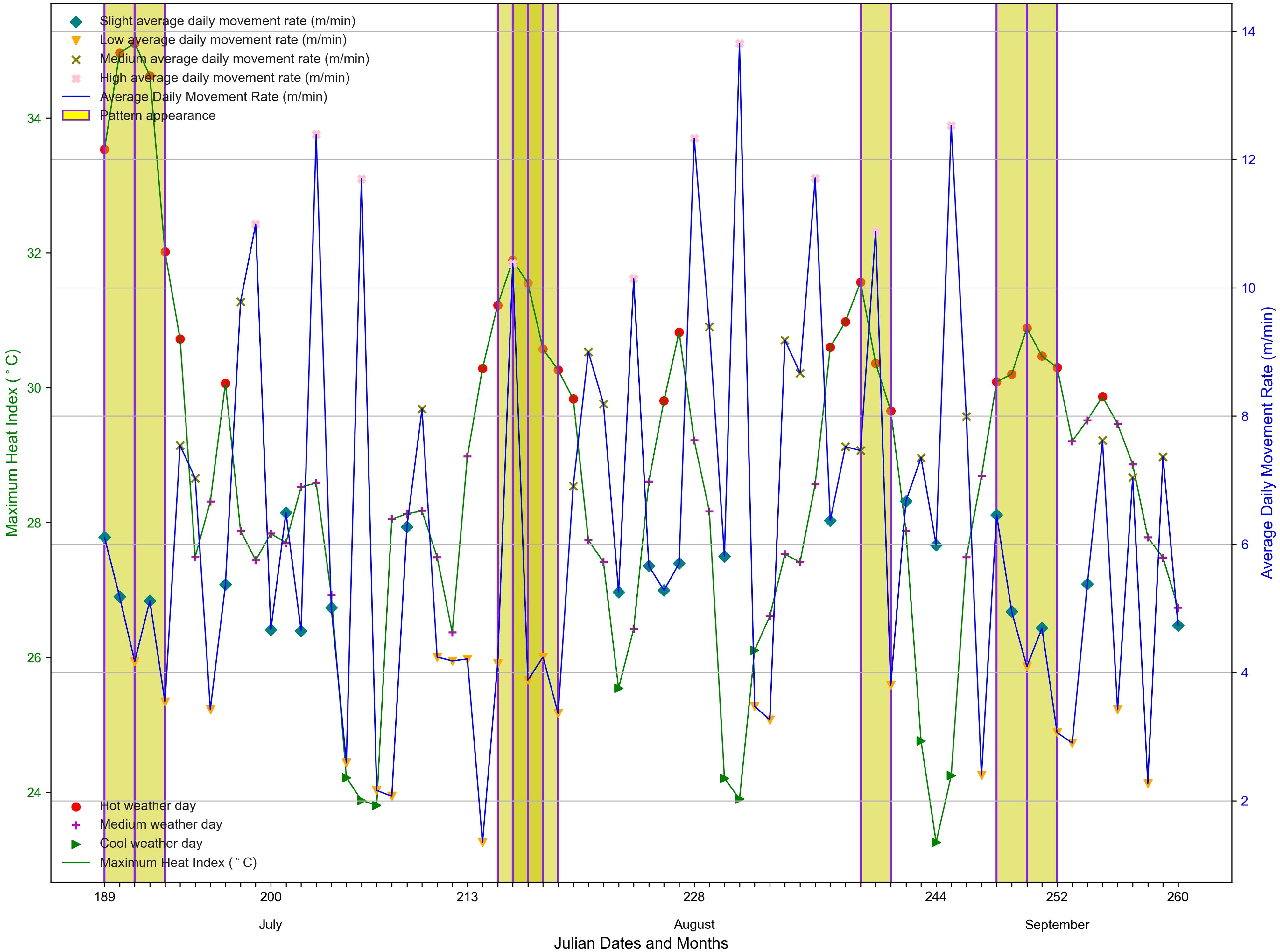
Figure 13. Three-day continuous patterns using the movement rate metric for cow ID 9128 in Trial 2 during period $P_1$, with detected patterns highlighted.

Figure 14

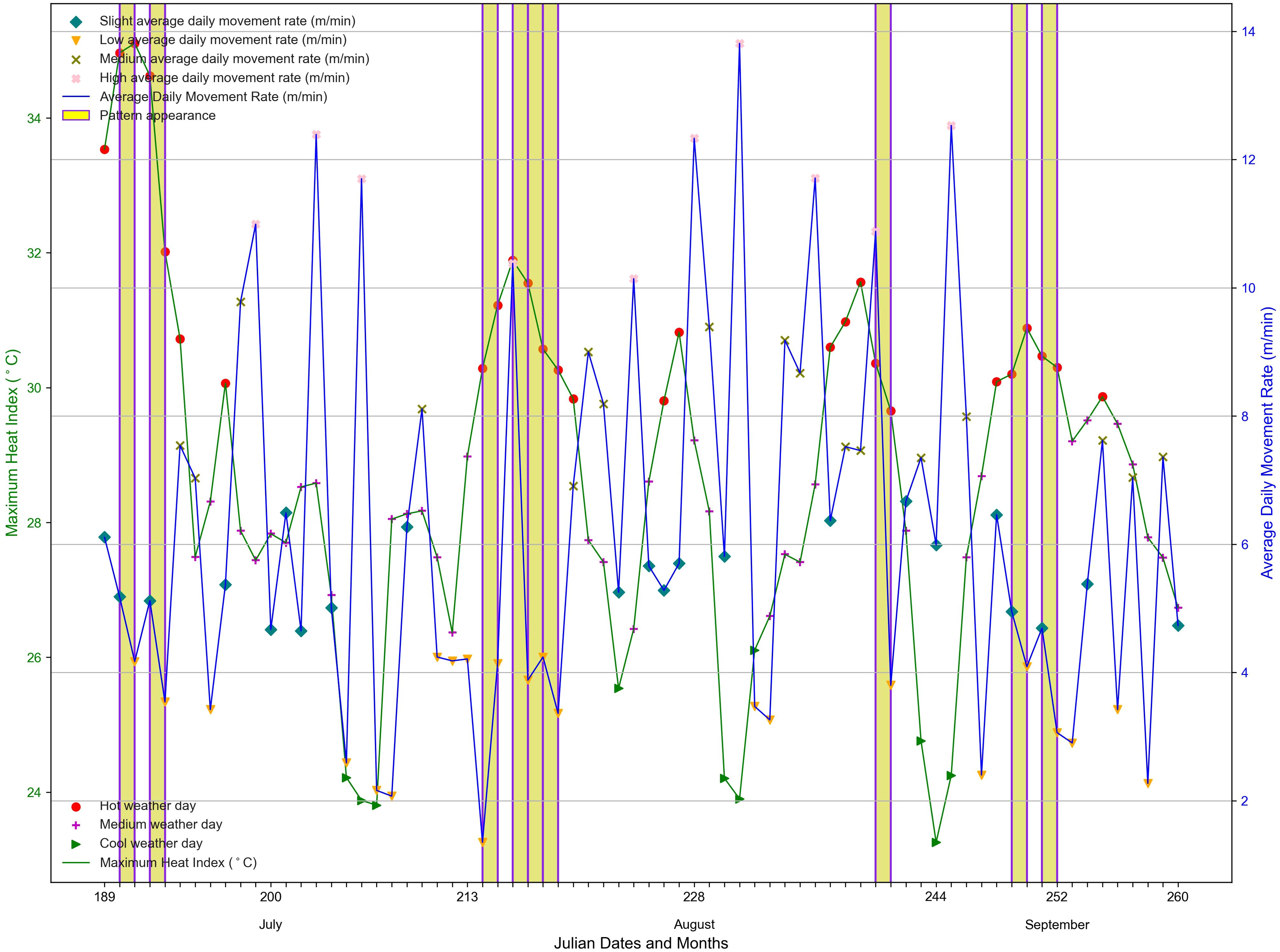
Figure 14. Two-day continuous patterns using movement rate metric for cow ID 9128 in Trial 2 during period $P_1$, with detected patterns highlighted.

Figure 15

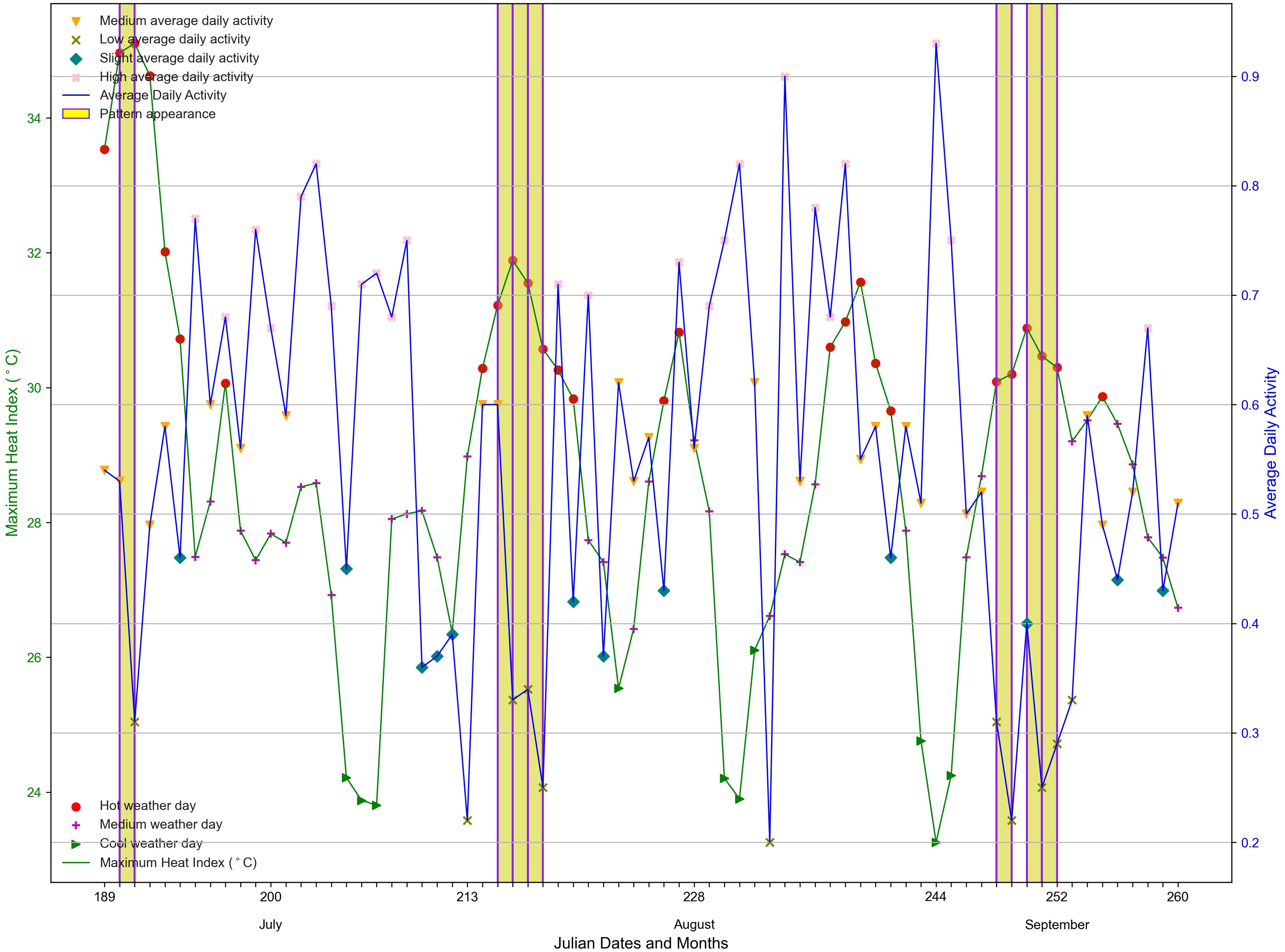
Figure 15. Two-day continuous patterns using activity metric for cow ID 67 in Trial 2 during period $P_1$, with detected patterns highlighted.

Table 5

Table 5. Percentage of cows with patterns during $P_1$ in Trial 2 for the behavior metrics: average daily movement rate, average daily activity and average daily distance travelled. Identification numbers (ID) of cows that display patterns in Trial 2 are listed.

During period P₂ (5:00 AM to 8:00 PM), no three-day continuous patterns were observed when using three behavior metrics. When average daily rate is used to represent the behavior, 42.86% of animals showed a two-day continuous pattern, while 57.14% of animals did not exhibit any continuous patterns (two-day, three-day or four-day) associated with hot weather and low movement rate. Similarly, CM-SPAM detected that 42.86% of animals showed two-day continuous pattern between hot weather and low activity, while the remaining animals showed no continuous patterns. Like in period P₁, CM-SPAM did not detect any continuous patterns between hot weather and reduced distance travelled to water, with 100% of animals showing no relationship (Table 6).

Table 6

Table 6. Percentage of cows with patterns during period $P_2$ of Trial 2 using the behavior metrics: average daily movement rate, average daily activity and average daily distance travelled from water. Identification numbers (ID) of cows displaying patterns are listed.

When the two-day continuous patterns were detected using movement rate during period P₁ for five cows out of seven cows, the frequency of decreased rates varied from 78% to 100%, with a mean of 92%. The minimum, maximum and mean values of average decrease in movement rate from the previous cool day within a week before a two-day continuous pattern started or the closest medium weather day to the end of the hot day in the pattern were 1.4 (m/min), 5.52 (m/min) and 3.76 (m/min), respectively. Among five cows, the average difference in movement rate from the cool day to rates during the hot period ranged from 1.4 (m/min) to 5.52 (m/min), with a mean of 3.18 (m/min). For the three cows showing the three-day continuous pattern in period P₁ using movement rate, the minimum, maximum and mean values for frequency of decrease were 75%, 100% and 92%, respectively. The average decrease in movement rate (the closest cool day within a week before a three-day continuous pattern began or the last medium weather day to the end of the hot day in the pattern) ranged from 1.4 (m/min) to 5.18 (m/min), with a mean of 3.78 (m/min). The minimum, maximum and mean values for the average difference for three-day continuous pattern from the previous cool day within a week before a three-day continuous pattern started or the closest medium weather day were 1.4 (m/min), 5.18 (m/min) and 3.23 (m/min), respectively (Table 7).

Table 7

Table 7. Comparison of movement rate changes between the closest cool day within seven days or the closest medium weather day before the first day of the two-day (or three-day) continuous pattern and the second day (or third day) of the two-day (or three-day) continuous pattern during period $P_1$ in Trial 2, including minimum, maximum and mean values for the frequency of decreased movement rate, average of movement rate decrease (prior to until the end), and overall movement rate differences (prior to versus hot period) for animals with two-day (or three-day) continuous patterns, along with the number of animals $n$ having the minimum and maximum values.

The binomial probability was calculated during P₁ period, based on the movement rate behavior metric over the two-day continuous patterns. With $m=2$, $n=105$, $k=49$, we find that $P(X=49)<0.0001$.

5 Discussion

In this study, CM-SPAM was applied to two separate summer trials conducted at the same pasture in different years, 2019 and 2021. Among three behavior metrics, the CM-SPAM algorithm successfully identified a frequent sequential pattern between hot weather and a decrease in movement rate in period $P_1$. The three-day continuous pattern showed that three consecutive hot days led to a decrease in movement rate on the third day during the morning and evening grazing bouts. Hahn (1999) describes how heat wave episodes (several days of hot weather) affected the ability of feedlot steers to maintain homeothermy. With several days of hot weather, many feedlot steers in the midwestern US succumbed to heat stress. Beatty et al. (2006) found that cattle exposed to sustained hot temperatures and high humidity levels in controlled climate rooms displayed increased respiration rates and core body temperature after several days. In addition, changes in blood chemistry (imbalance of acid-base and blood electrolytes) of the cattle occurred as a result of sustained high Temperature Humidity Index (THI). Heat index used in our study is similar, or identical, to THI. Although impacts of sustained hot weather are known to adversely affect feedlot cattle (Hahn, 1999) and cattle being transported in ships (Norris et al., 2003), little research has been conducted on the effect of consecutive days of hot weather (heat wave) on cattle grazing rangelands. This study uses data mining techniques to show that cattle behavior is affected by consecutive days of hot weather. Cattle in this study moved slower during the primary grazing bouts after two or more days of hot weather (high THI). Islam et al. (2021) suggested that GPS tracking could be used to remotely monitor cattle for heat stress. More time spent near shade and reduced activity might indicate that thermal conditions might be approaching levels that could adversely affect cattle. Nyamuryekung’e et al. (2021) reported that cattle moved slower during hot weather, but did not examine the effects of consecutive days of hot weather. Wade et al. (2024) found that the distance travelled by sheep each day decreased during a period of hot weather lasting three days.

Using period $P_1$ (morning and evening grazing bouts) is more effective in detecting the relationship between hot weather and a change in behavior compared to period $P_2$ (daylight) in both trials. Especially in Trial 1, most animals exhibited a three-day continuous pattern reduced movement rate during period $P_1$, when hot weather persisted for three days. This could be because period $P_1$ focuses on the two primary grazing bouts rather than all activity during daylight. Cattle typically reduce feed intake as a response to heat stress (Alves et al., 2020). The slower movement rates during the primary grazing bouts may reflect decreased grazing intensity and possibly reduced forage intake that would be expected as a response to high cumulative head.

In contrast to our expectations, we did not see reductions in activity or distance travelled from water after consecutive days of hot weather. It is unlikely that the cattle during the study period experienced heat stress. Temperature and humidity levels during the study were likely not great enough to induce heat stress. Instead, the cattle appeared to change at least some of their behaviors during grazing after 2 or more consecutive hot weather. The cattle were still moving during the early morning and evening periods (typical grazing bouts), but at slower rates. Our method for determining activity was based on a threshold of moving or resting over a 10-minute period. Cattle slowed down, but not perhaps the reduced rate was not enough to cross the threshold level and impact calculated activity levels. Distance travelled from water was evaluated as an indirect indicator of water intake. However, this metric may not be sensitive enough to monitor drinking activity. Cattle locations were recorded at 10-min intervals, but the typical time cattle spend drinking at the tank is only 1 or 2 minutes (Tobin et al., 2021b). Cattle may have drank multiple time while spending time near water, that our GPS tracking might not detect. More direct measures of remotely monitoring water intake such as flow meters or rumen boluses may be needed to evaluate the impact of consecutive days of hot weather on water intake for cattle grazing rangelands.

Compared to Trial 1 where most of animals (90.91%) showed a three-day continuous pattern, only about half of animals (42.86%) shows three-day continuous pattern in Trial 2. This may be because hot weather occurred less frequently in Trial 2 compared to Trial 1. During four months of Trial 1, the breaks between hot days was often shorter than during trial 2 (Figures 3, 4).

Movement rate was a more efficient metric than activity and distance travelled from water when analysing the relationship between cattle behavioral changes and continuous hot weather in both trials. In Trial 1, during the hot weather from Julian dates 236 to 244, animals with three-day and four-day continuous patterns had a consistently low average movement rates compared to animals without any these patterns (Figures 5, 6). It should be note that, in the summary comparison between Figures 5 and 6, the average movement rate of animals without patterns appears to be lower than that of animals with patterns. However, this does not impact our analysis because out method was applied to individual animals. The key focus of the comparison is not on the absolute values of movement rates, but rather changes and consistency of behavior (movement rate) of individual animals. This property, observed during the hot weather periods, indicates that animals that were not designated as having a pattern did not meet the minimum support threshold of 0.2 during period $P_1$. In other words, the three-day or four-day continuous pattern did not occur frequently enough to be detected as having a pattern, which explains the difference between the two groups. When examining individual cows, such as cow ID 105, which exhibited three-day (Figure 7) and four-day (Figure 8) continuous pattern, the movement rate metric identified these patterns frequently throughout the hot weather periods. On the other hand, when using the activity metric for cow ID 704 (Figure 9), the three-day continuous pattern was more variable. For cow ID 229 (Figure 10), the distance travelled from water metric did not reveal any connections between hot weather in July and cow behavior. During the longest seven-day continuous hot weather in Trial 2 from Julian dates 214 to 220, animals with two-day and three-day continuous patterns also exhibited consistently low average movement rates compared to those without any continuous patterns (Figures 11, 12). Once again, the key point is the consistency of individual animal responses between the two groups. When examining individual cows, for example cow ID 9128, using movement rate metric, three-day and two-day continuous patterns (Figures 13, 14) were frequently observed across the hot weather period. However, using activity metric for cow ID 67 (Figure 15), the two-day continuous pattern did not appear across all hot weather such as the hot period at the end of August.

Evaluation of changes in individual animals rather than using absolute metric values for detection of livestock behaviors has been recommended in several studies. Tobin et al. (2024) reported that individual sheep and individual accelerometers varied and that algorithms that evaluated changes of individuals would account for these sources of variation. Chang et al. (2022) reported that the accuracy of detecting cattle rumination improved 86% to 98% when using an individual animal model compared to a generic model for all animals. Using data mining, Trieu et al. (2025) was able to detect bovine ephemeral fever by evaluating the accelerometer streams of individual heifers and cows. In this study, the data mining approach must evaluate the changes in movement rates and other behavior metrics on an individual basis, because measured rates, activity and distances travelled from water vary among cows in both cool and hot weather. We are not aware of any studies that have used this data mining approach to study cumulative impacts of consecutive days of hot weather on cattle movements and activity. Data mining may be useful to identify patterns in cattle behavior that may be difficult to identify using traditional statistical techniques. The use of data mining for evaluating patterns in cattle behavior and responses to variable weather conditions deserves further exploration.

The mean values for both average decrease movement rates prior to and at the end of the hot period and the average difference in movement rate (before and during hot periods) that occurred in Trial 2 were lower than those in Trial 1. This is likely because Trail 2 had a shorter duration, and the length of hot weather periods were shorter. Cows may have varying tolerances to hot weather, and the movement rate often decreased by around 4 to 5 m/min with a maximum of 8 m/min during consecutive days of hot weather and patterns were detected (Trial 1). The mean value in frequency of decreased movement rates for three-day continuous pattern is higher than or equal to that of two-day and four-day continuous patterns. Additionally, the mean values for both the average decrease and the average difference in longer continuous patterns are slightly higher than in shorter ones. In Trial 1, the four-day continuous pattern shows a higher mean for both the average decrease in rate (prior to until the last day) and difference (average decrease in rate) compared to the three-day continuous pattern. Similarly, in Trial 2, the three-day continuous pattern shows a slightly higher mean values for decrease and difference than the two-day continuous pattern (Tables 4, 7). The smaller sample size in Trial 2 compared to Trial 1 also could potentially affect differences in movement rates between the two studies. However, the very low binomial probability values observed in both Trials 1 and 2 during period $P_1$ based on movement rate behavior indicate that the detected continuous patterns in our work are unlikely to have occurred by chance and are therefore considered statistically significant. As a result, these findings support our identification of frequent sequential patterns between consecutive day of hot weather conditions and cattle behavior. When considering both trials, these findings suggest that continued hot weather (long heat waves) may have a greater impact on grazing cattle than shorter heat waves.

6 Conclusion

In this study, GPS tracking and weather data were utilized to examine how hot weather affects cattle behaviors. K-means clustering was applied to categorize weather conditions into three levels (cool, medium, hot), while metrics from GPS tracking (movement rate, activity, and distance travelled from water) were categorized into four levels (low, slight, medium, high). CM-SPAM algorithm in data mining was applied to identify the relationship and successfully detected that consecutive hot days negatively affect cattle behavior, particularly reducing movement rate during the typical morning and evening grazing bouts. The data mining algorithm identified long-term responses, including two-day, three-day, or four-day continuous patterns in cattle movement in response to consecutive hot weather. Movement rates during the morning and evening grazing bouts decreased during 2 to 4 days consecutive days of hot weather. Data mining approaches may be a useful tool for evaluating behavioral impacts of heat waves. Ranchers should be aware that consecutive days of hot weather may have a greater impact on cattle behavior than a single day of hot conditions.

Data availability statement

The raw data supporting the conclusions of this article will be made available by the authors, without undue reservation.

Ethics statement

The protocol for this study was approved by the New Mexico State University Institutional Animal Care and Use Committee (approval number 2019-021). The study was conducted in accordance with the local legislation and institutional requirements.

Author contributions

LT: Conceptualization, Data curation, Formal analysis, Investigation, Methodology, Resources, Validation, Visualization, Writing – original draft, Writing – review & editing. DB: Conceptualization, Data curation, Funding acquisition, Investigation, Methodology, Project administration, Resources, Supervision, Validation, Visualization, Writing – original draft, Writing – review & editing. HC: Conceptualization, Formal analysis, Investigation, Methodology, Resources, Validation, Visualization, Writing – original draft, Writing – review & editing. TCS: Conceptualization, Funding acquisition, Project administration, Supervision, Writing – original draft, Writing – review & editing. CT: Data curation, Investigation, Methodology, Resources, Writing – original draft, Writing – review & editing. CO: Data curation, Investigation, Resources, Writing – original draft.

Funding

The author(s) declare financial support was received for the research and/or publication of this article. This project was funded in part by the Harold James Family Trust.

Conflict of interest

The authors declare that the research was conducted in the absence of any commercial or financial relationships that could be construed as a potential conflict of interest.

Generative AI statement

The author(s) declare that no Generative AI was used in the creation of this manuscript.

Any alternative text (alt text) provided alongside figures in this article has been generated by Frontiers with the support of artificial intelligence and reasonable efforts have been made to ensure accuracy, including review by the authors wherever possible. If you identify any issues, please contact us.

Publisher’s note

All claims expressed in this article are solely those of the authors and do not necessarily represent those of their affiliated organizations, or those of the publisher, the editors and the reviewers. Any product that may be evaluated in this article, or claim that may be made by its manufacturer, is not guaranteed or endorsed by the publisher.

References

Alves J. R. A., de Andrade T. A. A., de Medeiros Assis D., Gurjão T. A., de Melo L. R. B., and de Souza B. B. (2020). Productive and reproductive performance, behavior and physiology of cattle under heat stress conditions. J. Anim. Behav. Biometeorol. 5, 91–96. doi: 10.31893/2318-1265jabb.v5n3p91-96

Crossref Full Text | Google Scholar

Augustine D. J. and Derner J. D. (2013). Assessing herbivore foraging behavior with GPS collars in a semiarid grassland. Sensors 13, 3711–3723. doi: 10.3390/s130303711

PubMed Abstract | Crossref Full Text | Google Scholar

Ayres J., Flannick J., Gehrke J., and Yiu T. (2002). “Sequential pattern mining using a bitmap representation,” in Proceedings of the Eighth ACM SIGKDD International Conference on Knowledge Discovery and Data Mining. New York, NY: Association for Computing Machinery. 429–435.

Google Scholar

Bailey D. W. (2016). “Grazing and animal distribution,” in Animal welfare in Extensive Production Systems. The Animal Welfare Series (5M Publishing, Sheffield (UK), 53–77.

Google Scholar

Bailey D. W., Trotter M. G., Knight C. W., and Thomas M. G. (2018). Use of GPS tracking collars and accelerometers for rangeland livestock production research. Trans. Anim. Sci. 2, 81–88. doi: 10.1093/tas/txx006

PubMed Abstract | Crossref Full Text | Google Scholar

Beatty D. T., Barnes A., Taylor E., Pethick D., McCarthy M., and Maloney S. K. (2006). Physiological responses of Bos taurus and Bos indicus cattle to prolonged, continuous heat and humidity. J. Anim. Sci. 84, 972–985. doi: 10.2527/2006.844972x

PubMed Abstract | Crossref Full Text | Google Scholar

Becker C. A., Aghalari A., Marufuzzaman M., and Stone A. E. (2021). Predicting dairy cattle heat stress using machine learning techniques. J. Dairy. Sci. 104, 501–524. doi: 10.3168/jds.2020-18653

PubMed Abstract | Crossref Full Text | Google Scholar

Becker C. A., Collier R. J., and Stone A. E. (2020). Invited review: Physiological and behavioral effects of heat stress in dairy cows. J. Dairy. Sci. 103, 6751–6770. doi: 10.3168/jds.2019-17929

PubMed Abstract | Crossref Full Text | Google Scholar

Berman A. (2019). An overview of heat stress relief with global warming in perspective. Int. J. Biometeorol. 63, 493–498. doi: 10.1007/s00484-019-01680-7

PubMed Abstract | Crossref Full Text | Google Scholar

Bertsekas D. P. (1991). Linear network optimization. MIT Press, Cambridge.

Google Scholar

Bishop C. M. and Nasrabadi N. M. (2006). Pattern recognition and machine learning Vol. 4 (New York: Springer).

Google Scholar

Bradley P. S., Bennett K. P., and Demiriz A. (2000). Constrained k-means clustering. Microsoft. Res. Redmond. 20, 0.

Google Scholar

Branco T., de Moura D. J., de Alencar Nääs I., da Silva Lima N. D., Klein D. R., and Oliveira S.R. de M. (2021). The sequential behavior pattern analysis of broiler chickens exposed to heat stress. AgriEngineering 3, 447–457. doi: 10.3390/agriengineering3030030

Crossref Full Text | Google Scholar

Chang A. Z., Fogarty E. S., Moraes L. E., García-Guerra A., Swain D. L., and Trotter M. G. (2022). Detection of rumination in cattle using an accelerometer ear-tag: A comparison of analytical methods and individual animal and generic models. Comput. Electron. Agric. 192, 106595. doi: 10.1016/j.compag.2021.106595

Crossref Full Text | Google Scholar

Fournier-Viger P., Gomariz A., Campos M., and Thomas R. (2014). “Fast vertical mining of sequential patterns using co-occurrence information,” in Advances in Knowledge Discovery and Data Mining: 18th Pacific-Asia Conference, PAKDD 2014, Tainan, Taiwan, May 13-16, 2014. Proceedings, Part I 18. Eds. T. B., Z. Z.-H., C. A. L. P., K. H.-Y., Tseng V. S., and Ho Cham, Springer. 40–52. doi: 10.1007/978-3-319-06608-0_4

Crossref Full Text | Google Scholar

Fournier-Viger P., Lin J. C.-W., Kiran R. U., Koh Y. S., and Thomas R. (2017). A survey of sequential pattern mining. Data Sci. Pattern Recogn. 1, 54–77.

Google Scholar

Gonzalez-Rivas P. A., Chauhan S. S., Ha M., Fegan N., Dunshea F. R., and Warner R. D. (2020). Effects of heat stress on animal physiology, metabolism, and meat quality: A review. Meat. Sci. 162, 108025. doi: 10.1016/j.meatsci.2019.108025

PubMed Abstract | Crossref Full Text | Google Scholar

Gorczyca M. T. and Gebremedhin K. G. (2020). Ranking of environmental heat stressors for dairy cows using machine learning algorithms. Comput. Electron. Agric. 168, 105124. doi: 10.1016/j.compag.2019.105124

Crossref Full Text | Google Scholar

Hahn G. L. (1999). Dynamic responses of cattle to thermal heat loads. J. Anim. Sci. 77, 10–20. doi: 10.2527/1997.77suppl_210x

PubMed Abstract | Crossref Full Text | Google Scholar

Han J., Kamber M., and Pei J. (2011). Data Mining: Concepts and Techniques. 3rd ed (San Francisco: Morgan Kaufmann Publishers Inc).

Google Scholar

Islam M. A., Lomax S., Doughty A., Islam M. R., Jay O., Thomson P., et al. (2021). Automated monitoring of cattle heat stress and its mitigation. Front. Anim. Sci. 2, 737213. doi: 10.3389/fanim.2021.737213

Crossref Full Text | Google Scholar

Kilgour R. J., Uetake K., Ishiwata T., and Melville G. J. (2012). The behaviour of beef cattle at pasture. Appl. Anim. Behav. Sci. 138, 12–17. doi: 10.1016/j.applanim.2011.12.001

Crossref Full Text | Google Scholar

Knight C. W., Bailey D. W., and Faulkner D. (2018). Low-cost global positioning system tracking collars for use on cattle. Rangeland. Ecol. Manage. 71, 506–508. doi: 10.1016/j.rama.2018.04.003

Crossref Full Text | Google Scholar

Liakos K. G., Busato P., Moshou D., Pearson S., and Bochtis D. (2018). Machine learning in agriculture: A review. Sensors 18, 2674. doi: 10.3390/s18082674

PubMed Abstract | Crossref Full Text | Google Scholar

Mia N., Sarker T., Halim M. A., Alam A., Ali M. S., Rahman M. M., et al. (2025). Machine learning overview and its application in the livestock industry. Meat. Res. 5, 1-10. doi: 10.55002/mr.5.1.109

Crossref Full Text | Google Scholar

Mluba H. S., Atif O., Lee J., Park D., and Chung Y. (2024). Pattern Mining-Based pig behavior analysis for health and welfare monitoring. Sensors 24, 2185. doi: 10.3390/s24072185

PubMed Abstract | Crossref Full Text | Google Scholar

Napolitano F., De Rosa G., Chay-Canul A., Álvarez-Mac\’\ias A., Pereira A. M. F., Bragaglio A., et al. (2023). The challenge of global warming in water buffalo farming: physiological and behavioral aspects and strategies to face heat stress. Animals 13, 3103. doi: 10.3390/ani13193103

PubMed Abstract | Crossref Full Text | Google Scholar

Nawaz M. S., Fournier-Viger P., Nawaz M. Z., Chen G., and Wu Y. (2022). MalSPM: Metamorphic malware behavior analysis and classification using sequential pattern mining. Comput. Secur. 118, 102741. doi: 10.1016/j.cose.2022.102741

Crossref Full Text | Google Scholar

Nawaz M. S., Fournier-Viger P., Shojaee A., and Fujita H. (2021). Using artificial intelligence techniques for COVID-19 genome analysis. Appl. Intell. 51, 3086–3103. doi: 10.1007/s10489-021-02193-w

PubMed Abstract | Crossref Full Text | Google Scholar

Norris R. T., Richards R. B., Creeper J. H., Jubb T. F., Madin B., and Kerr J. W. (2003). Cattle deaths during sea transport from Australia. Aust. Vet. J. 81, 156–161. doi: 10.1111/j.1751-0813.2003.tb11079.x

PubMed Abstract | Crossref Full Text | Google Scholar

Nyamuryekung’e S. (2024). Transforming ranching: Precision livestock management in the Internet of Things era. Rangelands 46, 13–22. doi: 10.1016/j.rala.2023.10.002

Crossref Full Text | Google Scholar

Nyamuryekung’e S., Cibils A. F., Estell R. E., McIntosh M., VanLeeuwen D., Steele C., et al. (2021). Foraging behavior and body temperature of heritage vs. commercial beef cows in relation to desert ambient heat. J. Arid. Environ. 193, 104565. doi: 10.1016/j.jaridenv.2021.104565

Crossref Full Text | Google Scholar

Nyamuryekung’e S., Cibils A. F., Estell R. E., VanLeeuwen D., Steele C., Estrada O. R., et al. (2020). Do young calves influence movement patterns of nursing raramuri criollo cows on rangeland? Rangeland. Ecol. Manage. 73, 84–92. doi: 10.1016/j.rama.2019.08.015

Crossref Full Text | Google Scholar

Pektaş A. (2018). Mining patterns of sequential Malicious APIs to detect malware. Int. J. Netw. Secur. Its. Appl. (IJNSA). 10, 1-9. doi: 10.2139/ssrn.3247606

Crossref Full Text | Google Scholar

Shine P. and Murphy M. D. (2021). Over 20 years of machine learning applications on dairy farms: A comprehensive mapping study. Sensors 22, 52. doi: 10.3390/s22010052

PubMed Abstract | Crossref Full Text | Google Scholar

St-Pierre N. R., Cobanov B., and Schnitkey G. (2003). Economic losses from heat stress by US livestock industries. J. Dairy. Sci. 86, E52–E77. doi: 10.3168/jds.S0022-0302(03)74040-5

Crossref Full Text | Google Scholar

Tan P.-N., Steinbach M., and Kumar V. (2016). Introduction to data mining (Bew Delhi: Pearson Education India).

Google Scholar

Tobin C., Bailey D. W., Stephenson M. B., and Trotter M. G. (2021a). Temporal changes in association patterns of cattle grazing at two stocking densities in a central Arizona rangeland. Animals 11, 2635. doi: 10.3390/ani11092635

PubMed Abstract | Crossref Full Text | Google Scholar

Tobin C., Bailey D. W., and Trotter M. G. (2021b). Tracking and sensor-based detection of livestock water system failure: A case study simulation. Rangeland. Ecol. Manage. 77, 9–16. doi: 10.1016/j.rama.2021.02.013

Crossref Full Text | Google Scholar

Tobin C., Bailey D., Wade C., Trieu L. L., Nelson K., Oltjen C., et al. (2024). Evaluation of experimental error in accelerometer monitoring: variation among individual animals versus variation among devices. Smart. Agric. Technol. 7, 100432. doi: 10.1016/j.atech.2024.100432

Crossref Full Text | Google Scholar

Trieu L. L., Bailey D. W., Cao H., Son T. C., Macor J., Trotter M. G., et al. (2025). Potential of accelerometers to remotely early detect bovine ephemeral fever in cattle using pattern mining. Trans. Anim. Sci. 9, txaf008. doi: 10.1093/tas/txaf008

PubMed Abstract | Crossref Full Text | Google Scholar

Wade C., Trotter M., Chang A., Steele C., Prihodko L., and Bailey D. W. (2024). Use of global positioning system tracking to assess landscape distribution in extensive small ruminant operations☆. Rangeland. Ecol. Manage. 94, 29–37. doi: 10.1016/j.rama.2024.01.010

Crossref Full Text | Google Scholar