 Zhongtao Xie
 Yisong Wang
 Lei Yang
 Renyan Feng
- 1State Key Laboratory of Public Big Data, Key Laboratory of Advanced Medical Imaging and Intelligent Computing of Guizhou Province, College of Computer Science and Technology, Guizhou University, Guiyang, China
- 2College of Mathematical Sciences, Minzu Normal University of Xingyi, Guiyang, China
- 3School of Information, GuiZhou University of Finance and Economics, Guiyang, China
Circumscription is an important logic framework for representing and reasoning common-sense knowledge. With efficient implementations for circumscription, including circ2dlp and aspino, it has been widely used in model-based diagnosis and other domains. We propose a notion of minimal reduct for propositional circumscription and prove a characterization theorem, i.e., that the models of a circumscription can be obtained from the minimal reduct of the circumscription. With the help of the minimal reduct, a new method circ-reduct for computing models of circumscription is presented. It iteratively computes smaller models under set inclusion (if possible), and the minimal reduct is used to simplify the circumscription in each iteration. The algorithm is proved to be correct. Extensive experiments are conducted on circuit diagnosis ISCAS85, random CNF instances, and some industrial SAT instances for the international SAT competition. These results demonstrate that the minimal reduct is effective in computing circumscription models. Compared to the widely used circumscription solver circ2dlp using the state-of-the-art answer set programming solver clingo, our algorithm circ-reduct achieves significantly shorter CPU time. Compared with aspino using glucose as the internal SAT solver and unsatisfiable core analysis technique, our algorithm achieves better CPU time for random and industrial CNF benchmarks, while it is comparable for circuit diagnosis benchmarks.
1 Introduction
Recent breakthroughs in large language models (LLMs) and foundation models have spurred an intense interest in integrating symbolic reasoning with data-driven learning to improve interpretability and controllable inference. Within this trend, classical logic techniques are being revisited as essential tools to provide strong guarantees and structured reasoning capabilities that purely statistical methods often lack (Ryu et al., 2025; Ye et al., 2023; Pan et al., 2023; Olausson et al., 2023; Callewaert et al., 2025).
Beyond classical approaches, non-monotonic reasoning has attracted renewed attention because it naturally captures default assumptions and common-sense knowledge that must be revised when new information arrives (Reiter, 1988). Recent ASP-based reasoning optimizations illustrate this synergy (Yang et al., 2023; Zeng et al., 2024; Rajasekharan et al., 2023). In addition, recent data-driven clustering methods continue to inspire logical inference. For example, automated cluster elimination guided by high-density points (Hu et al., 2025) and constrained clustering with weak label prior (Zhang et al., 2023) illustrate how structural knowledge can guide efficient search.
A prominent formalism for non-monotonic reasoning is circumscription, originally introduced by McCarthy for common-sense reasoning. Circumscription minimizes the extension of specific predicates, embodying a closed-world assumption where statements not known to be true are considered false (McCarthy, 1980). To increase the knowledge representation capabilities of ordinary circumscription, Lifschitz proposed parallel circumscription incorporating atoms that are allowed to vary (Lifschitz, 1985). Circumscription has received considerable attention in areas such as knowledge formalization (McCarthy, 1986; Lifschitz, 1986), common-sense reasoning (Wang et al., 2015; Alviano, 2019), diagnosis (Wotawa and Kaufmann, 2022; Metodi et al., 2014; Stern et al., 2012; Friedrich et al., 1999), planning (Sierra-Santibáñez, 2000), and privacy protection applications (Ogunniye and Kökciyan, 2023).
Despite its theoretical and practical significance, circumscription presents substantial computational challenges. It was shown that determining whether a circumscription has a model is NP-complete, verifying whether an interpretation is a model of a given circumscription is coNP-complete, and determining whether a formula is a logical consequence of a circumscription is -complete (Eiter and Gottlob, 1993; Cadoli and Lenzerini, 1994). Consequently, efficiently computing models for propositional circumscription remains a formidable task. To the best of our knowledge, the main approach for computing circumscription models involves translating circumscriptions into (general) disjunctive logic programs under answer set semantics (ASP in short) (Gelfond and Lifschitz, 1988) such that the answer sets of the logic program correspond to the models of circumscription, allowing the use of efficient ASP solvers.
Sakama and Inoue (1995) proposed a method for translating circumscription into general disjunctive logic programs; however, this method requires the calculation of characteristic clauses, which can lead to exponential explosion. to translate finite first-order circumscription without varying predicates into first-order ASP. Although varying predicates can be eliminated in circumscription (Cadoli et al., 1992), the worst case can still result in exponential explosion. All the above translations for propositional circumscriptions either introduce fresh (predicate) symbols, or may result in exponential explosion. The ones for computing first-order circumscription primarily focus on translating first-order circumscription (or second-order theories) into first-order theories under certain constraints (Przymusinski, 1989; Doherty et al., 1997), for which there is no efficient implementation to the best of our knowledge.
Another alternative approach involves translating circumscription into the propositional satisfiability problem (SAT). Lee and Lin proposed a method that employs loop formulas and completions to translate circumscriptions into propositional theories. However, this method requires finding loop formulas, and the number of loop formulas may be exponential (Lee and Lin, 2006). Notably, enumerating models of circumscriptions is also interesting. For this purpose, Alviano proposed an unsatisfiable core analysis and implemented a solver aspino making use of the SAT solver glucose (Alviano, 2017), but this approach only employs solver which support cardinality constraints.
Recently, Wang et al. proposed the concept of minimal reduct for answer set programs. It substantially improves the minimal model decomposition of propositional theories (Angiulli et al., 2022), in addition to a new characterization for answer sets of logic programs (Zhang et al., 2021; Wang et al., 2023). Informally, the minimal reduct of a logic program P w.r.t. an interpretation M is obtained by replacing all atoms that are false under M in P with false.
In this study, we extend the notion of minimal reduct from answer set programming to (parallel) propositional circumscriptions and show that the minimal reduct preserves models of circumscription. With the help of minimal reduct and efficient SAT solvers, two approaches for computing and enumerating models of circumscriptions are presented, namely circ/circ-reduct and circ-enum. Extensive experimental results show that circ/circ-reduct is comparable with the state-of-the-art circumscription solvers circ2dlp and aspino.
The main contributions of this study are as follows:
• We introduce the concept of minimal reduct for propositional circumscription and establish its theoretical soundness by proving that it preserves satisfiability. Intuitively, the minimal reduct allows a circumscription formula to be simplified with respect to a given interpretation while keeping its essential models unchanged. This provides a new foundation for developing efficient SAT-based algorithms for computing circumscription models;
• We propose two sound algorithms for computing and enumerating models of propositional circumscriptions: circ, circ-reduct and circ-enum, respectively;
• We implement the aforementioned algorithms based on an open-source SAT solver (Cai et al., 2022) and conduct extensive experiments on diagnosis, random and industrial CNF formulas SAT competitions. We show that the two methods are comparable with the state-of-the-art methods circ2dlp and aspino.
The structure of the study is as follows: In Section 2, we review the necessary background knowledge; In Section 3, we propose minimal reduct for circumscription; In Section 4, we discuss the enumeration algorithm circ-enum; Section 5 details our experiments, demonstrating that the circ and circ-reduct methods can effectively compute propositional circumscription models; finally, we conclude the study and outline future research directions in Section 7.
2 Circumscription
In the section, we briefly recall the basic notions and notations of circumscription (McCarthy, 1980; Lifschitz, 1985; McCarthy, 1986):
Assume that the propositional symbols of the propositional language form a finite set of atoms . A literal l is either an atom p or the negation of an atom ¬p, while a clause α is a disjunction of literals:
When n = 0, α≡⊥. For convenience, the clause α can also be written as the set of literals {l1, ⋯ , ln}. We denote and α− = {p∣¬p∈α}. A clause theory A is a set of finite clauses.
If , we denote , ¬S = {¬p∣p∈S}, ∨S = ∨p∈Sp, and ∧S = ∧p∈Sp. The notions of formula, theory, interpretation, model, satisfaction (⊧), non-satisfaction (⊭), equivalence (≡), etc., in the propositional language are the same as in classical propositional logic. We denote uar(e) as the set of all atomic symbols appearing in the formula (or theory) e.
Abusing the notation, a tuple (t1, …, tk) is usually written as {t1, …, tk} when there is no confusion from its context. The expression A(P, Q) denotes a formula/theory that contains atoms from P∪Q, where P, Q are disjoint sets of atoms; we denote A(P) as A(P, Q) when Q = ∅. When X, Y are tuples of the same length as P, Q respectively, A(X, Y) denotes the formula (or theory) obtained from A by simultaneously replacing the atoms from P, Q with the corresponding atoms from X, Y.
Example 1. Let A({p, q}, {r}) = (p∨¬q)∧(r∨¬p). Then A({x, y}, {z}) = (x∨¬y)∧(z∨¬x);
Let P = {p1, …, pn} and Q = {q1, …, qn} be two sets of atoms.
• P ≤ Q denotes ∧1 ≤ i ≤ n(pi→qi);
• P = Q denotes ∧1 ≤ i ≤ n(pi↔qi);
• P<Q denotes (P ≤ Q)∧¬(P = Q).
The basic idea of circumscription is to minimize the set of atoms assigned true as much as possible while keeping certain atoms fixed, thereby obtaining a “minimal” model.
Definition 1. Let A be a formula, and let P, Z be disjoint sets of atoms. The circumscription of P in formula A with Z allowed to vary, denoted as CIRC[A; P; Z], is the following formula:
where X, Y are fresh disjoint tuples of atoms with the same length as P, Z respectively. When Z = ∅, CIRC[A; P; Z] is shortened as CIRC[A; P].
In Definition 1, the P is called the minimizing set, the Z is called the varying set, and the set of remaining atoms is called the fixing set. Intuitively, the circumscription CIRC[A; P; Z] is to minimize (under set inclusion) the interpretation of P, while fixing the interpretation for . The varying set Z consists of atoms whose truth values may change freely during this minimization, and as long as the original formula A remains satisfied, their assignment can be arbitrary.
Let P and Z be disjoint sets of atoms, M, M′ be two interpretations (sets of atoms). We use M ≤P; ZM′ to denote
• M∩P⊆M′∩P, and
• M\(P∪Z) = M′\(P∪Z).
If M ≤P; ZM′ holds but M′ ≤P; ZM does not, we denote this as M<P; ZM′. When Z = ∅, M ≤P; ZM′ is shortened to M ≤PM′, and M<P; ZM′ shortened to M<PM′.
Definition 2 (Circumscription model). Given a formula A(P, Z), for any interpretation M, if M is a model of A(P, Z) and there exists no model M′ of A(P, Z) satisfying M′ < P; ZM, then M is a model of CIRC[A(P, Z);P; Z].
Intuitively, given a propositional formula φ, its circumscription in a set of minimizing atoms is the formula having only the models of φ that do not assign minimizing atoms to true unless necessary. For example, consider the formula A in Example 1, it is not hard to verify that {p, q, r}⊧A but {p, q, r}⊭CIRC[A; {p, q, r}] because ∅⊧A and ∅ < {p, q, r}{p, q, r}. In fact, for any disjoint sets P, Q of atoms, ∅ is a model of CIRC[A; P; Q].
Example 2 (Circumscription in common-sense reasoning). Consider the use of circumscription in common-sense reasoning. Let
which states that birds normally fly unless an abnormality (ab) occurs. When computing Circ[K; ab; fly], we obtain three models: {bird, fly}, {fly}, and ∅.
Here, ab is minimizing, meaning that we prefer situations where no abnormality occurs. Indeed, in all three models ab is false, which intuitively corresponds to “no abnormality happens.”
• The first model can be read as: it is a bird, and it flies.
• The second and third models correspond to situations where it is not a bird, in which case flying may or may not hold.
In this setting: Fixing atoms can be understood as conditions that partition the cases under consideration. Minimizing atoms typically represents abnormalities, which are assumed to be false unless evidence suggests otherwise. Varying atoms corresponds to reasoning outcomes that may change depending on the situation.
The next corollary easily follows from Definition 2.
Corollary 1. Let A be a formula and M⊆𝒜. Then
1. M⊧CIRC[A; var(A)] if and only if M is a minimal model of A.
2. M⊧CIRC[A; ∅; var(A)] if and only if M⊧A.
3. CIRC[A; P; Z] has a model if and only if A has a model.
The next example shows that circumscription is a generalization of the theory of minimal models.
Example 3. Let A = {p∨q}, 𝒜 = {p, q}. It's not hard to verify the following:
• CIRC[A; {p, q}] has two models {p} and {q}, that are exactly the minimal models of A.
• CIRC[A; {p};{q}] has only one model {q} since {q} < {p};{q} {p}.
• CIRC[A; ∅; {p, q}] has three models {p}, {q} and {p, q}.
3 Minimal reduct for circumscriptions
In this section, we introduce minimal reduct for circumscriptions. This reduct, based on the inherent structure of circumscription models, achieves efficient model search through iterative formula reduct and simplification.
Definition 3 (Minimal reduct). Given a clause theory A(P, Z) and M⊆𝒜, the minimal reduct of A w.r.t. M, P and Z,1 is the set of clauses consisting of, for each α∈A,
such that
1. ,
2. , and
3. .
The minimal reduct of the circumscription CIRC[A; P; Z] w.r.t. M⊆𝒜, denoted as CRed[A; P; Z, M], is the circumscription CIRC[Red(A; P; Z, M);P∩M; Z].
For convenience, we denote Equation 3 by Red[α; P; Z, M]. If one of the conditions (a), (b) or (c) in Definition (Equation 3) does not hold, then clause (Equation 3) does not belong to Red[A; P; Z, M]. In this case, we define Red[α; P; Z, M] = ⊤.
Thus, if there is no clause in A that satisfies one of the conditions (a), (b) and (c) then Red[A; P; Z, M]≡⊤.
Intuitively, the minimal reduct simplifies clauses with respect to a given interpretation. For a given clause and interpretation, if some atoms in the fixing set make the clause true, or if some atoms in the minimizing set that are false make the clause true, then the clause is reduced to ⊤. Otherwise, the clause is further simplified to retain only the varying atoms and those atoms in the minimizing set that are assigned true, so that minimization can continue on these relevant literals.
The next lemma follows from Definition 3 easily.
Lemma 1. Let M⊆𝒜, α(P, Z) be a clause, and A(P, Z) be a clause theory.
1. If M⊭α, then Red[α; P; Z, M] = α+∩Z∪¬(α−∩(P∪Z)).
2. var(Red[A; P; Z, M])⊆P∩M∪Z.
The following example illustrates the notions of minimal reduct CRed and Red.
Example 4. Let P = {p, q}, Z = {z}, M = {q, a}, M′ = {p}, A1(P, Z) consists of
It is evident that M⊧A1 and . We have:
• Red[A1; P; Z, M] = {z∨q}, because α1 does not satisfy the condition (a) of Definition 3, and α3 does not satisfy condition (c) of Definition 3.
• CRed[A1; P; Z, M] = CIRC[z∨q; {q};{z}], which has only one model {z}, and it is also a model of CIRC[A1; P; Z].
• , which has a unique minimal model {z}; , which has only one model {z}.
Intuitive explanation. The distinction between fixing and minimizing atoms plays a crucial role here. For any M⋆ such that M⋆<P; ZM, the truth values of the fixing atom in {a} remain unchanged between M⋆ and M. For the minimizing atoms in {p, q}, if an atom is false in M, it must also be false in M⋆. The varying atom z, on the other hand, may freely change across models. These assumptions drive the simplification of clauses in the reduct.
Take Red[A1; P; Z, M] = {z∨q} as an example: For α1 = ¬p∨¬z, since p is false in M, ¬p is always true; hence α1 is satisfied and can be reduced to ⊤; For α2 = z∨q, the values of z and q cannot be determined from M, so the whole clause is retained; For α3 = ¬q∨p∨a, since a is true in M, the clause is always satisfied and reduces to ⊤.
Thus, only α2 survives in the reduct, yielding {z∨q}.
Next, we discuss the properties of minimal reduct. This lemma establishes the fundamental correspondence between a clause and its minimal reduct under a given interpretation M. It explains how the satisfaction of a reduced clause by an interpretation M′ reflects the satisfaction of the original clause by a combined interpretation that agrees with M on the fixing atoms while possibly minimizing atoms in P. In particular, Lemma 2 guarantees that the reduct construction preserves the semantic relationship between M and M′ with respect to the partial order ≤P; Z. This property is crucial for proving that the minimal reduct maintains the models of the original theory (Theorem 1) and, consequently, that the overall reduction process is sound with respect to the circumscription semantics.
Lemma 2. Let P, Z, M be the ones in Definition 3, the clause α satisfies conditions (a)-(c) in Definition 3, and M′⊆𝒜. Then
1. ;
2. α−∩(M∩P∪Z) = α−∩(P∪Z);
3. M′⊧Red[α; P; Z, M] if and only if .
The next theorem shows that the minimal reduct for clause theories preserves the models of A that have the same assignment for fixing atoms, while the minimizing atoms may be minimized further.
Theorem 1. Let A(P, Z) and M be the ones in Definition 3, and M′⊆𝒜. Then M′⊧Red[A; P; Z, M] if and only if .
Informally, if a set of atoms M′ is a model of Red[A; P; Z, M], then one can construct a model of A that agrees with M on the fixing atoms and agrees with M′ on varying atoms, while the minimizing atoms in M are further minimizing in terms of M′.
Example 5. Let M = {a, p, q}, A(P; Z) = {¬a∨p∨¬q, q∨¬p}, where P = {p, q} and Z = ∅. It can be readily verified that M is a model of A(P, Z), and Red[A; P; Z, M] = {p∨¬q, q∨¬p}. The intersection is {a}. We consider the following two cases:
1. When M′ = ∅, we have M′⊧Red[A; P; Z, M]. Furthermore, , which is a model of A.
2. When M′ = {p}, we have M′⊭Red[A; P; Z, M]. The resulting set is , which is not a model of A.
The following theorem demonstrates how to construct a model of CIRC[A; P; Z] from a model M′of CRed[A; P; Z, M].
Theorem 2. Let A(P, Z) be a clause theory, and M′, M⊆𝒜. Then M′⊧CRed[A; P; Z, M] if and only if .
Example 6. Let A(P; Z) = {p∨¬q, q∨¬p, p}, where P = {p} and Z = ∅. It is not hard to verify that CIRC[A; P; Z] has a unique model {p, q}. We consider the following cases:
1. Let M1 = {p}. Then Red[A; P; Z, M1] = {p, ¬p}, which is obviously unsatisfiable, so CRed[A; P; Z, M1] has no model. In fact, CIRC[A; P; Z] also has no such model M which assigns all fixing atoms false, i.e., .
2. Let M2 = {p, q}. Then Red[A; P; Z, M2] = {p}, so CRed[A; P; Z, M2] has a unique model {p}. It's easy to see that {p, q}⊧CRed[A; P; Z, M2], and in fact, there is only one M′ such that .
The next follows easily from Theorem 2.
Corollary 2. Let A(P, Z) be a clause theory, Z = ∅, M, M′⊆𝒜, M be a model of A(P, Z). The following statements are equivalent to each other:
i. M′⊧CRed[A; P; Z, M];
ii. M′ is a minimal model of Red[A; P; Z, M];
iii. .
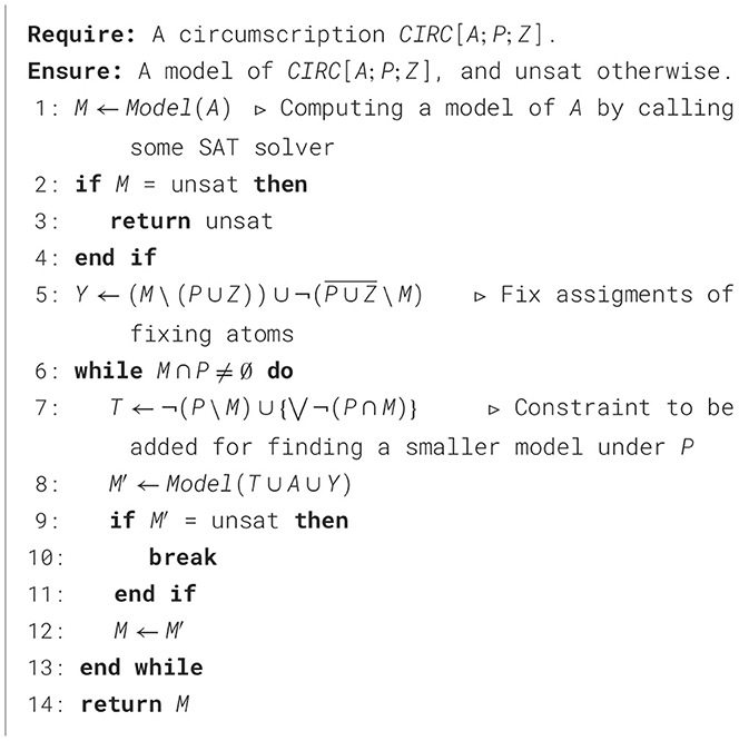
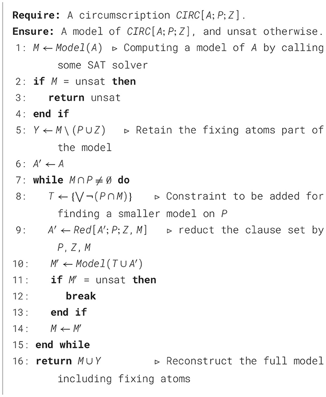
Note that a simple approach to compute circumscription models is to iteratively compute subset minimal models by calling an SAT solver in terms of Definition 1. With the help of Theorem 2, we obtain a new approach to compute circumscription models. It is based on the simple one and makes use of the minimal reduct to simplify the circumscription in each iteration. The typical one and the new one are named as circ and circ-reduct, respectively. They are presented as Algorithms 1, 2, while Model(.) extracts a model by calling an SAT solver which returns unsat if its input is unsatisfiable. This algorithm can be viewed as an extension of the works by Koshimura et al. (2009) and (Ben-Eliyahu and Dechter 1993). Specifically, when the fixing set is empty, this algorithm aligns with the methods described in Koshimura et al. (2009) and (Ben-Eliyahu and Dechter 1993).
Algorithm 1. circ(A, P, Z).
Algorithm 2. circ-reduct (A, P, Z).
Intuitively, in Algorithm 1, the set Y determines the truth values of the fixing atoms of the model. Specifically, as long as M′⊧Y, the assignment of these atoms in M′ remains the same as in M. The set T ensures that fewer atoms in the minimizing set are assumed to be true. That is, M′∩P⊂M∩P if M′⊧T. Therefore, the main idea of this algorithm is to find an assignment with fewer true atoms in the minimizing set, while keeping the assignment of the fixing atoms, and satisfying the original theory A. Note that if the theory A is unsatisfiable, we assume that Model(A) returns unsat; otherwise, it returns a model of A. This algorithm calls the SAT solving procedure at most |P|+1 times in the worst case.
Theorem 3. Algorithm circ(A; P; Z) is correct. That is, if circ(A, P, Z) returns unsat, then there exists no model of CIRC[A; P; Z]; otherwise, the set of atoms returned by circ(A, P, Z) is a model of CIRC[A; P; Z].
The idea of Algorithm 1 is to compute circumscription models by adding block clauses, whereas Algorithm 2 computes them by reducing the size of the clause set. Clearly, Algorithm 2 also calls the SAT solver |P|+1 times in the worst case.
Theorem 4. Algorithm circ-reduct(A, P, Z) is correct. That is, circ-reduct(A, P, Z) returns a model of CIRC[A; P; Z] if A is satisfiable; otherwise, circ-reduct(A, P, Z) returns unsat.
The following example intuitively demonstrates the computation process of Algorithms 1, 2.
Example 7 (Continuation of Example 4). Here 𝒜 = {p, q, z, a}. Note that P = {p, q}, Z = {z}, and the clause theory A1(P, Z) consists of
(a) The execution process of Algorithm 1 on A1, P, Z is as follows:
1. Assume that Model(A1) line 1 returns M = {q, a}, then at line 5, Y = {a};
2. In the first iteration of the WHILE loop, T = {¬p}∪{¬q} (line 7);
M′ = {a, z} (line 8, at this time the only model of T∪A∪Y is M′);
M′≠ unsat (line 9);
M = M′ (line 12);
the loop ends (line 6), since M∩P = ∅;
3. At line 14, return M = {z, a}. It's easy to see that M⊧CIRC[A1; P; Z].
(b) The execution process of Algorithm 2 on A1, P, Z is as follows:
1. Assume that Model(A1) line 1 returns the model M = {q, a}, then at line 5, Y = {a};
2. In the first iteration of the WHILE loop, T = {¬q} (line 8);
A′ = {z∨q} (line 9);
M′ = {z} (line 10, at this time the only model of T∪A′ is M′);
M′≠ unsat (line 11);
M = M′ (line 14);
the loop ends (line 7), since M∩P = ∅;
3. At line 16, return M = {z, a}. It is easy to see that M⊧CIRC[A1; P; Z].
3.1 Complexity analysis
In this section, we analyze the time complexity of the two algorithms presented: Algorithm 1 (circ) and Algorithm 2 (circ-reduct). The complexity mainly depends on the number of SAT solver calls and the auxiliary set operations. Let the input clause theory A contain n clauses over m atoms. While propositional satisfiability has a worst-case complexity of O(2m), modern SAT solvers typically perform much better in practice due to sophisticated heuristics.
3.1.1 Time complexity of algorithm (circ)
The complexity can be analyzed as follows:
• Initial SAT call: computing an initial model M of A requires one SAT solver call, in O(2m) time.
• Set operations: constructing Y by combining and negating subsets of M involves O(m) operations.
• Main loop: the loop iterates at most |P| times. In each iteration:
- Constructing T takes O(|P|) time.
- A SAT solver call on T∪A∪Y costs O(2m) time.
Thus, Algorithm 1 makes at most |P|+1 SAT calls, with polynomial overhead in m. The overall complexity is O(m·2m) since |P| ≤ m.
3.1.2 Time complexity of algorithm circ-reduct
Algorithm 2 refines models by applying reducts until minimality is achieved:
• Initial SAT call: one SAT call on A, in O(2m) time.
• Set operations: constructing Y requires O(m) operations.
• Main loop: the loop executes at most |P| times. In each iteration:
- Constructing T requires O(|P|) time.
- Applying the reduct Red[A′; P; Z, M] requires at most O(n·m) operations.
- A SAT solver call on T∪A′ runs in O(2|Z|+|M∩P|) time in the worst case.
Therefore, the loop contributes at most O(2|Z|+|P|) complexity. Including the initial SAT call, the total complexity is O(2m) since |Z|+|P| ≤ m.
Both algorithms are dominated by the number of SAT solver calls. Algorithm circ requires at most |P|+1 SAT solver calls, while Algorithm circ-reduct may involve additional clause reductions. In practice, modern SAT solvers significantly mitigate the theoretical exponential bound, and our empirical results confirm that the overhead of reduct operations is manageable.
4 Circumscription models enumeration
In this section, we further investigate the model enumeration problem for circumscriptions with the help of the algorithm circ and circ-reduct.
Let P, Z be disjoint finite subsets of 𝒜 and M⊆𝒜. By 𝒮(M, P, Z) we denote the formula
If P and Z are sets of “minimizing” and “varying” atoms, respectively, then the counter-models of constraint (Equation 4) correspond to the interpretations that are P, Z-greater than M, as shown by the next lemma. Thus, it can be used to exclude such M in the search for circumscription models.
Lemma 3. Let P, Z be disjoint finite subsets of 𝒜 and M⊆𝒜. Then, for each M′⊆𝒜, if and only if M ≤ P; ZM′.
Example 8. Consider the clause theory A(P, Z) = {α1:p∨q, α2:p∨r} where P = {p, q, r}, Z = ∅, and M = {p} We observe the following:
• .
• For any M′ such that p∈M′, we have and M ≤ P; ZM′.
The next corollary easily follows from the above Lemma 3. It shows that the constraint (Equation 4) can indeed be used to compute some new circumscription models different on varying atoms.
Corollary 3. Let A(P, Z) be a clause theory, M be a model of CIRC[A; P; Z] and M′⊆𝒜. Then, if and only if M\Z≠M′\Z and M′⊧CIRC[A; P; Z].
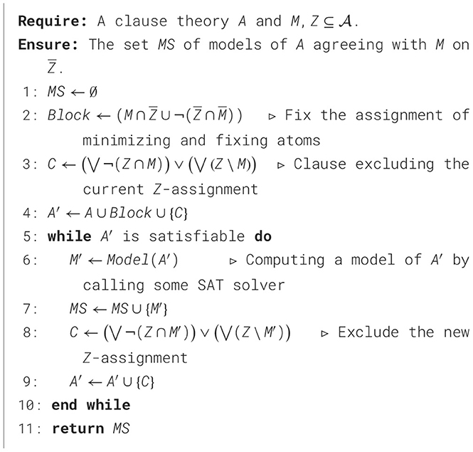
According to Corollary 3, we propose the algorithm circWithZ to iteratively compute such models that are merely different on given varying atoms of Z. The following example shows how this algorithm is involved in computing such models.
Example 9. Let A = {α1:p∨q, α2:a∨¬p, α3:q∨z}, P = {p, q}, Z = {z}, and M = {a, q, z}. It is evident M⊧A. The computation process using circWithZ(A, M, Z) is as follows:
1. At line 1, MS = ∅;
2. At line 2, Block = {a, q, ¬p};
3. At line 3, C = {¬z};
4. At line 4 A′ = {p∨q, a∨¬p, q∨z, a, q, ¬p, ¬z};
5. In the first iteration of the WHILE loop, M′ = {a, q} (line 6)
MS = {{a, q}} (line 7);
C = {z} (line 8);
A′ = {p∨q, a∨¬p, q∨z, a, q, ¬p, ¬z, z} (line 9);
the loop ends (line 5), since A′ is satisfiable;
6. At line 11 returns MS = {{a, q}}.
The correctness of the algorithm circWithZ is guaranteed by the next theorem.
Theorem 5. Algorithm 3 is sound and complete.
Algorithm 3. circWithZ(A,M,Z).
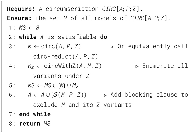
We are now in the position to present the algorithm of enumerating circumscription models, as shown by Algorithm 4. Informally, this algorithm circ-enum iteratively computes a circumscription model and then immediately enumerates all models that merely differ from the just-computed model. The core concept underlying this approach is akin to the strategies outlined in prior works, such as those by Dvořák et al. (2015) and (Niskanen and Järvisalo 2020).
Algorithm 4. circ-enum(A,P,Z).
The correctness of circ-enum is guaranteed by the next theorem.
Theorem 6. Algorithm 4 is sound and complete.
The next example illustrates how circ-enum can be used to compute all circumscription models.
Example 10. Let A = {α1:p∨q, α2:a∨¬p, α3:q∨z}, P = {p, q}, and Z = {z}. The computation steps for circ-enum(A, P, Z) are detailed below:
1. In the first iteration of the WHILE loop, we assume that circ (or circ-reduct) returns M = {a, q, z} at line 3, then
Mz = {{a, q}} (line 4);
MS = {{a, q, z}, {a, q}} (line 5);
A = {p∨q, a∨¬p, q∨z, ¬a∨¬q} (line 6);
enter next iteration of the WHILE loop, since A is satisfiable;
2. In the second iteration of the WHILE loop, we assume that circ (or circ-reduct) returns M = {q, z} at line 3, then
Mz = {{q}} (line 4);
MS = {{a, q, z}, {a, q}, {q, z}, {q}} (line 5);
A = {p∨q, a∨¬p, q∨z, ¬a∨¬q, ¬q∨a} (line 6);
the loop ends (line 2), since A is unsatisfiable;
3. At line 8 returns MS = {{a, q, z}, {a, q}, {q, z}, {q}}.
5 Experimental results
Based on one of the state-of-the-art SAT solvers LSTech-Maple,2 all three algorithms circ, circ-reduct, circ-enum have been implemented. This SAT solver integrates stochastic local search techniques into conflict-driven clause learning (CDCL) SAT solvers and keeps its completeness (Cai and Zhang, 2022; Cai et al., 2022).
To evaluate their performance, we selected three categories of benchmarks: model-based circuit diagnosis, random propositional circumscription, and various industrial test cases from the SAT competition.
We compare the three algorithms implemented circ and circ-reduct with aspino3 and circ2dlp4 The experimental environment includes a Linux server running Ubuntu 20.04 with an AMD EPYC 7742 CPU and 1007 GB of memory. The implementation and experimental data have been uploaded to GitHub.5
5.1 Note on unsatisfiable instances
For formulas that are unsatisfiable, the SAT solver invoked in the first step immediately reports UNSAT, so the core circumscription procedure is not executed. Consequently, the runtime and other performance metrics on such inputs are determined almost entirely by the underlying SAT solver, with the overhead of our circ/circ-reduct algorithms being negligible. UNSAT search itself can be costly, typically involving extensive branching and conflict analysis; approaches that extract unsatisfiable cores may introduce additional overhead, which likewise stems from the solver rather than our method.
In this section, we only foucs on CPU time, the memory will be reported in Supplementary material 2.
It should be emphasized that the issues observed with circ2dlp stem from minor implementation inconsistencies rather than from any flaw in the underlying theory of circumscription. In particular, circ2dlp may occasionally produce incorrect results when handling fixing atoms. For example, for A = {x1∨x2∨x3}, P = ∅, and Z = ∅, the rules generated from A by circ2dlp are not recognizable by clasp. Likewise, for A = {α1:x1∨x3, α2:¬x1∨x2} and P = {x2, x3}, circ2dlp returns only {x3} as the unique model of CIRC[A; P], whereas {x1, x2} is also a valid model. To handle such cases in practice, we developed the tool cnf2any,6 which eliminates fixing atoms following the method proposed by (de Kleer and Konolige 1989).
5.2 Integration with existing SAT frameworks
Our algorithms invoke an external SAT solver through its standard CNF interface. Modern SAT solvers such as Maple, Glucose, and MiniSat all provide C/C++ source code and well-documented APIs, so circ and circ-reduct can be integrated into other systems or embedded in larger software projects with minimal effort. This integration requires only routine engineering work–such as linking against the solver library or calling its incremental interface–and does not affect the theoretical correctness or performance guarantees of our approach. We emphasize that our implementation intentionally targets SAT solvers via CNF interfaces. Attempting to integrate the method with an ASP toolchain (e.g., clingo) is, in our assessment, not practically feasible without changing the problem or incurring prohibitive costs.
5.3 Model-based circuit diagnosis
Formally, a model-based circuit diagnosis is a triple D = (SD, COMP, OBS), where SD is a propositional theory that describes the circuit system, COMP is a finite set of components (atoms), and OBS is a set of literals representing system observations. A component set M is a diagnosis of D if and only if SD∪OBS∪{¬Ab(a)∣a∈COMP\M}∪{Ab(c)∣c∈M} is satisfiable, where Ab(a) indicates that component a is abnormal. If M is a diagnosis of D and no proper subset of M is a diagnosis of D, then M is referred to as a minimal diagnosis of D (Reiter, 1987).
We used 11 standard ISCAS85 circuits 7 as our benchmarks. These circuit descriptions are translated into CNF formulas that serve as the system description SD, the circuit gates as the components COMP, and random assignments of circuit inputs and outputs as the observations OBS. The minimal diagnoses of D = (SD, COMP, OBS) correspond to the circumscription models of CIRC[SD∪OBS; COMP]. It is important to note that all circuit components are the minimizing atoms of CIRC[SD∪OBS; COMP], while all other propositional symbols are treated as varying atoms of CIRC[SD∪OBS; COMP].
For each circuit, we randomly generated 20 observation instances, ran 5 times for each instance, with a CPU time limit of 1,800 s, and calculated the average CPU time for solved instances. The experimental results are presented in Table 1. The best CPU time for each circuit is in bold face. It can be seen that both circ and circ-reduct significantly outperform circ2dlp, and are comparable with aspino. In particular, while circ and circ-reduct solved all the 20 instances of the c6828 circuit, aspino ran out of 30 min for 19 instances. Additionally, the minimal reduct seems not very helpful for the benchmark since circ and circ-reduct have very similar average CPU time.
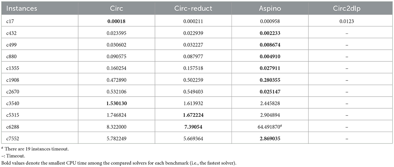
Table 1. The average CPU time in seconds for minimal circuit diagnosis.
5.4 Random circumscriptions
We examined our algorithms on random CNF instances whose number of atoms in 𝒜 ranges from 50 to 1000 with an interval of 50, and clause-to-atom ratios are from 3 to 5 with an interval of 0.5. The CNF instances were generated using the method proposed by Amendola et al. (2020). We generated 10 instances for each combination, resulting in 20 × 5 × 10 = 1000 random circumscriptions in total.
For each CNF φ over , we created random circumscriptions CIRC[φ; P; Z] by randomly selecting disjoint subsets P and Z from , with |P| and |Z| set to 10%, 30%, or 50% of .
Tables 2, 3 present the average CPU time in seconds and the number of satisfiable and unsatisfiable instances solved by circ, circ-reduct, aspino, and circ2dlp within a 2-hour CPU time limit, respectively. It can be observed that both circ and circ-reduct significantly outperform aspino and circ2dlp by four orders of magnitude on satisfiable instances. Our methods solved a few hundred instances more than both aspino and circ2dlp.
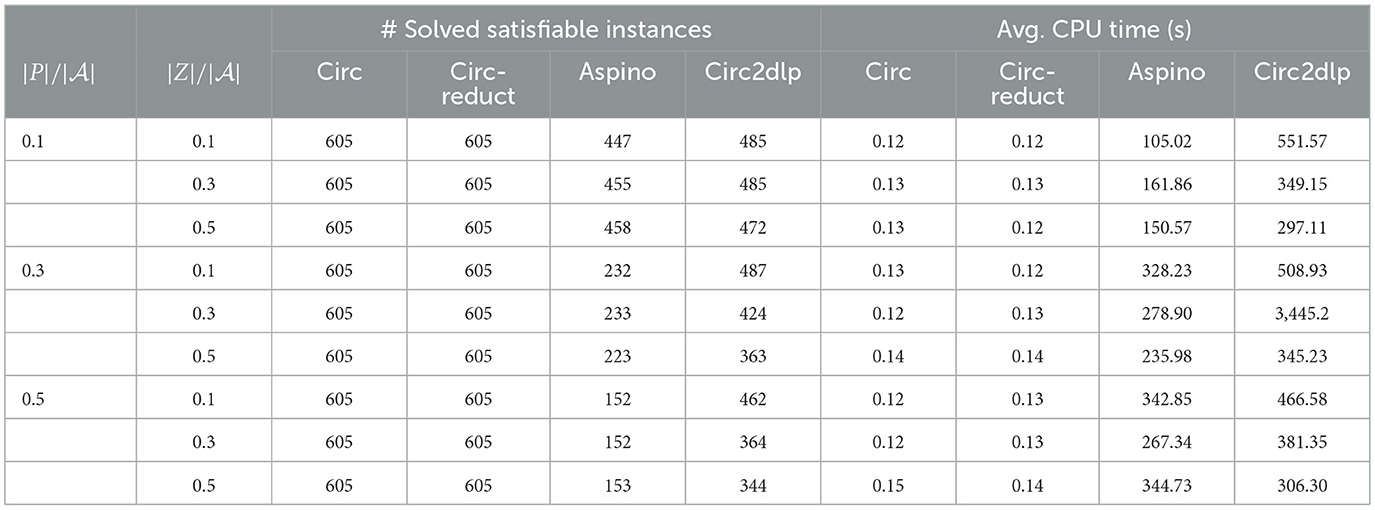
Table 2. The number of solved satisfiable instances and the average CPU time in seconds for random circumscriptions.
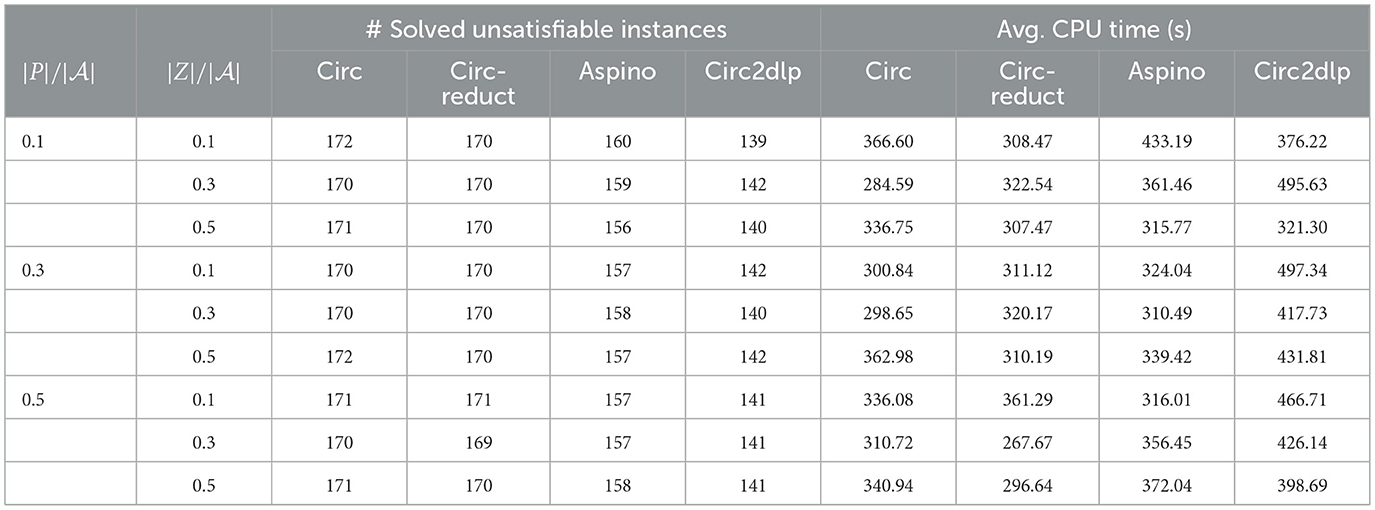
Table 3. The number of solved unsatisfiable instances and the average CPU time in seconds for random circumscriptions.
For unsatisfiable instances, circ and circ-reduct also demonstrate an advantage by solving a greater number of instances, though there is no big difference in the average CPU time.
Beyond average CPU time, we also analyze how the clause set shrinks across reduct rounds. For each circumscription instance we record the number of clauses Cr after round r and report the remaining-clauses ratio ρr = Cr/C0 (lower is better). Since different instances may terminate after different numbers of rounds, the statistic at round r aggregates only those instances that reached at least r rounds (no imputation). Figure 1 shows per-round pruning trajectories split by |P|/|𝒜|∈{0.1, 0.3, 0.5} (three panels), with curves stratified by |Z|/|𝒜|∈{0.1, 0.3, 0.5}; bands indicate IQR across instances. Figure 2 overlays all nine (|P|/|𝒜|, |Z|/|𝒜|) settings in one panel for a global view.
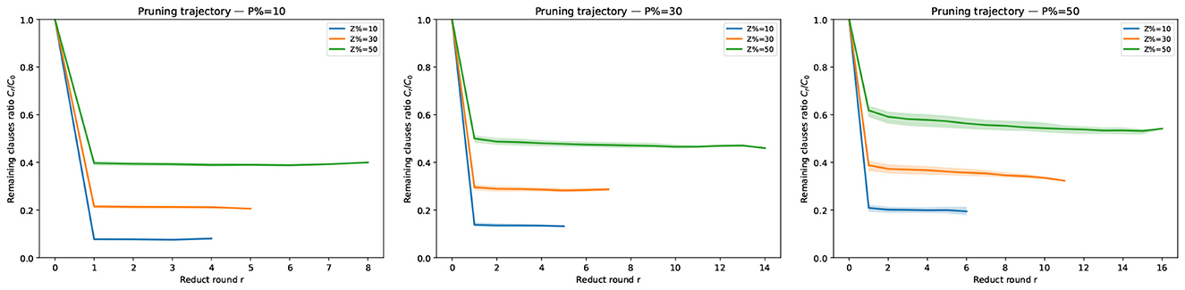
Figure 1. Per-round pruning trajectories by |P|/|𝒜|. Each panel fixes |P|/|𝒜| and shows the median remaining-clauses ratio Cr/C0 across reduct rounds, with curves stratified by |Z|/|𝒜|∈{0.1, 0.3, 0.5}. Shaded bands indicate the interquartile range (IQR, 25th–75th percentile) across instances at each round; solid curves show the median. At round r, statistics aggregate only instances that reached at least r rounds.
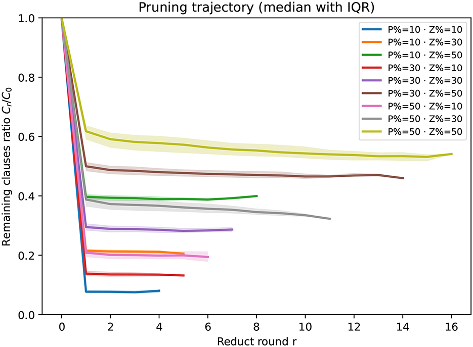
Figure 2. Overall pruning trajectories across (|P|/|𝒜|, |Z|/|𝒜|). Median remaining-clauses ratio Cr/C0 with IQR bands (25th–75th percentile) across instances; lower curves indicate stronger pruning. Curves flatten more slowly as |P|/|𝒜| or |Z|/|𝒜| increases, indicating more reduct rounds before convergence.
Guided by the trajectories in Figures 1, 2, we observe:
1. Holding |Z|/|𝒜| (resp. |P|/|𝒜|) fixed, the total number of reduct rounds increases as |P|/|𝒜| (resp. |Z|/|𝒜|) grows, i.e., larger fixed or varying sets require more rounds before convergence. (ii) Across all configurations the first reduct yields the smallest remaining ratio (largest pruning step).
2. Quantitatively, after the first round we observe ρ1≈0.10 at (|Z|/|𝒜|, |P|/|𝒜|) = (0.1, 0.1) (about 90% pruned), whereas even in the least favorable setting (0.5, 0.5) the first round still leaves ρ1≈0.60 (about 40% pruned). These trends are consistent across all clause densities considered.
5.5 Circumscription of industrial CNF benchmarks
We choose moderate size industrial CNF benchmarks from SAT competitions.8 They are Collatz and Johnson from SAT-2019, Giraldez from SAT-2016, and crypto and grieu from SAT-2007. While both Collatz and Johnson contain 19 instances, Giraldez has 29 instances, crypto and grieu have 10 instances. To generate circumscription instances, we applied the same strategy to generate P and Z as described in Section 5.4. We report the metrics only for satisfiable instances, since there is no big difference for unsatisfiable instances, as shown in Table 3 for random CNFs.
Please note that while aspino, circ and circ-reduct specify varying and fixing predicates at the end of input files, circ2dlp specifies varying predicates and fixing predicates in the command line as arguments. Due to the very large number of atoms or clauses in Collatz and crypto, circ2dlp either outputs a “argument list too long” or runs out of time on the two benchmarks, while aspino always runs out of time. For clarity, the experimental results on Collatz and crypto are not reported in detail for aspino and circ2dlp. Tables 4–8 present the test results for the solved satisfiable instances by circ, circ-reduct, aspino, and circ2dlp in Collatz, crypto, Johnson, Giraldez, and grieu benchmarks, respectively. The experimental results further confirm the effectiveness of circ and circ-reduct compared with aspino and circ2dlp, while there is no much difference between circ and circ-reduct.
• There is no big difference between circ and circ-reduct in terms of the number of solved instances or the average CPU time per instance. Both circ and circ-reduct solved exactly the same number of satisfiable instances for all benchmarks excluding Johnson, for which circ-reduct solved slightly less number of instances than that of circ in at most 2. For the benchmark crypto the overall average CPU time of circ (resp. circ-reduct) is 840.37 (resp. 803.90), and for the benchmark Giraldez it is 63.77 (resp. 59.92). For the benchmark Callatz, the overall average CPU time of circ (resp. circ-reduct) is 1417 (resp. 1,437).
• circ and circ-reduct solved more instances than aspino and circ2dlp for the benchmarks Johnson, Giraldez and grieu. For the benchmark Giraldez, both circ and circ-reduct solve 18 instances, while aspino solved two instances, see Table 7. For the benchmark Johnson, circ and circ-reduct solved 5–7 instances, while circ2dlp solved up to two instances, see Table 6. There are similar results for the benchmark grieu, see Table 8.
• Both circ and circ-reduct have usually less average CPU time than aspino and circ2dlp for the solved instances of the benchmarks Johnson, Giraldez and grieu, even though circ and circ-reduct solved more instances.
• It seems that for all mentioned computing methods the ratios of minimizing and varying predicates over the signature do not have a distinguishing effect on the computing efficiency.
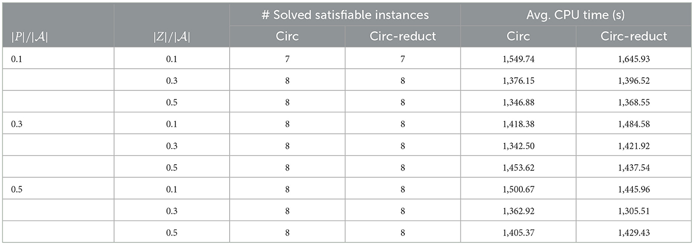
Table 4. The number of solved satisfiable instances and average CPU time in seconds for Collatz.
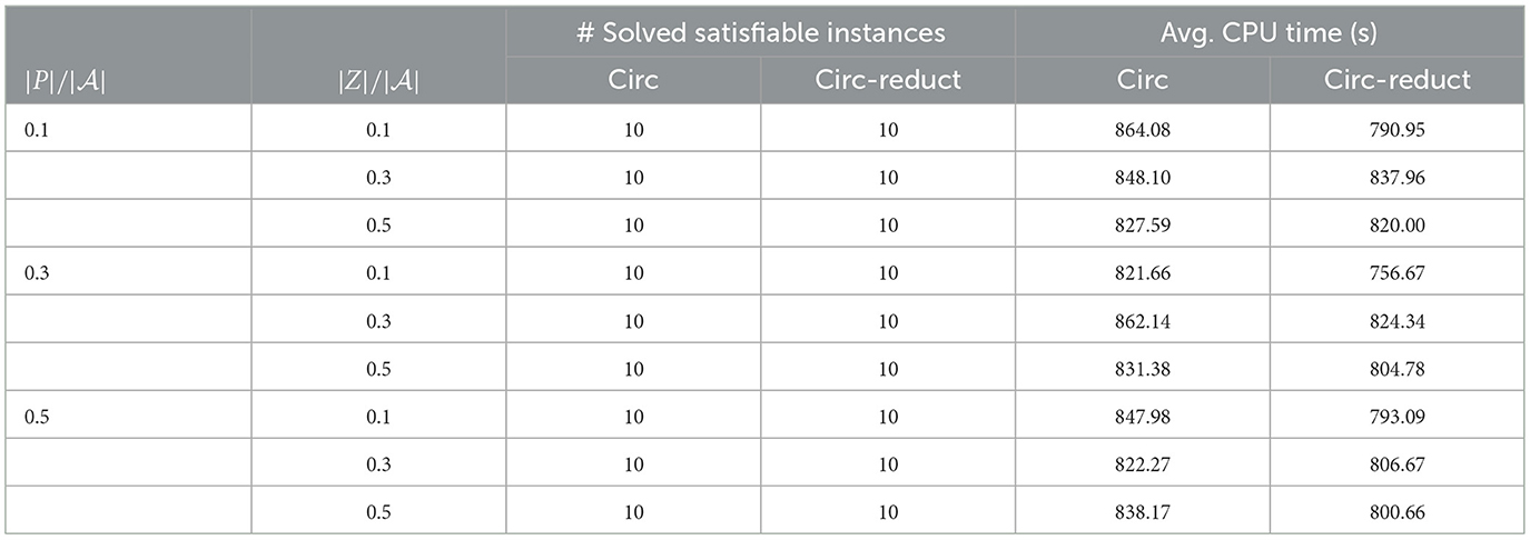
Table 5. The number of solved satisfiable instances, average CPU time in seconds for crypto.
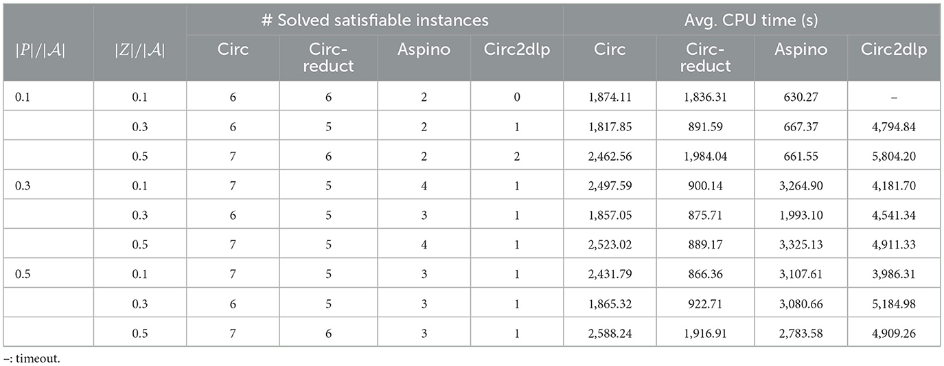
Table 6. The number of solved satisfiable instances and average CPU time in seconds for Johnson.
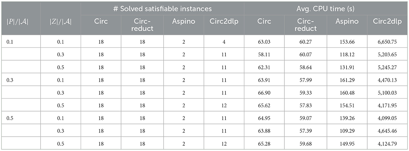
Table 7. The number of solved satisfiable instances and average CPU time in seconds for Giraldez.
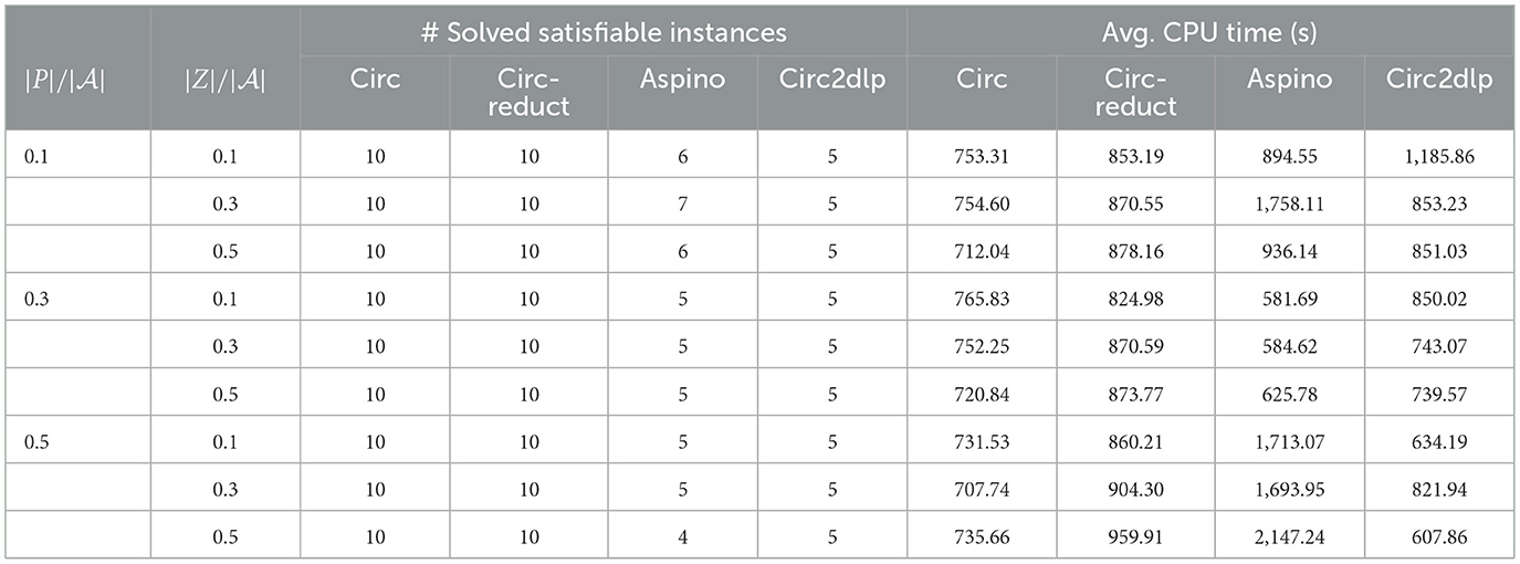
Table 8. The number of solved satisfiable instances and the average CPU time in seconds for grieu.
For enumerating circumscription models, we have implemented the algorithm circ-enum calling circ or circ-reduct and evaluated it against all the above benchmarks. In this case, the CPU limit is set up to 30 min. The experimental results do not show a remarkable difference between circ-enum and aspino, while they outperform circ2dlp. For instance, circ2dlp enumerates all the 60 models for the diagnosis of circuit c17, aspino enumerates 0 models for the diagnosis of circuit c6288. For the random CNFs, aspino solved a larger number of instances than that of circ-enum. For the benchmark grieu, circ-enum computed more instances than aspino. We do not report these experimental results in detail for simplicity. Interested readers may refer to the experiments in the above github link.
6 Related work
Since the introduction of circumscription, the challenge of efficiently computing circumscription models has become a significant focus of research.
Currently, methods for computing circumscription are categorized into two classes: translating circumscriptions into logic programs (under stable model semantics) or leveraging SAT solvers.
6.1 Translating circumscription to logic programming
Early research concentrated on simplifying circumscription. Lifschitz (1985) proposed eliminating mutable predicates in circumscription in 1985, but this method introduced existential quantifiers. In 1988, Yuan and Wang extended this approach to specific cases, but both methods suffered from exponential growth (Yuan and Wang, 1988). Later, in 1992, Cadoli introduced a technique for eliminating variable predicates in circumscription (Cadoli et al., 1992); however, this method focused on inferring formulas from circumscription rather than transforming it. In 1989, Kleer and Konolige developed a method for eliminating fixing predicates in circumscription (de Kleer and Konolige, 1989).
In 1995, Sakama and Inoue proposed translating circumscription into a general disjunctive logic program (Sakama and Inoue, 1995), where the stable models correspond to circumscription models, but their method required the computation of characteristic clauses, leading to potential clause explosion. In 2008, Oikarinen and Janhunen addressed prioritized circumscription in the propositional case by translating it into a disjunctive logic program (Oikarinen and Janhunen, 2008), and implementing the tool circ2dlp. Similarly, in 2011, Gebser et al. developed metasp (Gebser et al., 2011), a general implementation technique using meta-programming, which reuses existing ASP systems to capture various forms of qualitative preferences among answer sets. This approach also enables the computation of circumscription in the propositional case without fixing predicates.
In 2014, Wan et al. developed cfo2lp, which translates first-order circumscription into a logic program, outperforming both circ2dlp and metasp on circuit diagnosis problem (Wan et al., 2014).
6.2 Translating circumscription to SAT
Inspired by loop formulas in computational logic programs (Lee and Lifschitz, 2003; Lin and Zhao, 2004), (Lee and Lin, 2006) proposed using loop formulas and completions to compute circumscription in the propositional case. However, the number of loops can grow exponentially, and the method requires eliminating existential quantifiers, making it potentially exponentially complex. In 2017, Alviano introduced an approach for enumerating propositional circumscription models using unsatisfiable core analysis, with the SAT solver functioning as a search engine (Alviano, 2017). This method also requires the introduction of auxiliary variables during computation.
In the propositional case, when the fixing predicate set is empty, the circumscription model is equivalent to the P-minimal model. Giunchiglia and Maratea (2006) proposed a tool in 2006 based on the Davis-Logemann-Loveland (DLL) algorithm to solve SAT-related optimization problems, including P-minimal models. In 2009, Koshimura introduced a SAT-based algorithm for computing P-minimal models (Koshimura et al., 2009). However, a common limitation of these approaches is their inability to handle circumscription containing fixing predicates.
A notable SAT-based approach relevant to our work is the counterexample-guided abstraction refinement (CEGAR) framework for propositional circumscription proposed by Janota et al. (2010). While their primary focus is on solving the entailment problem through iterative abstraction refinement, their CEGAR-based algorithm shares conceptual similarities with our constraint refinement process in Algorithms 1, 4. Specifically, both approaches employ counterexamples to guide the incremental refinement of constraints. In the context of circumscription, CEGAR excels at computing the set of variables assigned false in all models of a circumscribed formula.
6.3 Summary
Table 9 provides a comprehensive summary of the primary methodologies for computing circumscription models, delineating their core strategies and inherent limitations. Due to the absence of reported complexity analyses for certain methods, complexity metrics are excluded from the comparison. Furthermore, as the evaluation is restricted to comparisons with aspino and circ2dlp, performance metrics are not included. In general, the circ/circ-reduct approach demonstrates superior performance compared to aspino, while the circ and circ-reduct methods exhibit equivalent performance. Moreover, our proposed approach scales to significantly larger input instances than previously reported methods, highlighting its strong scalability.
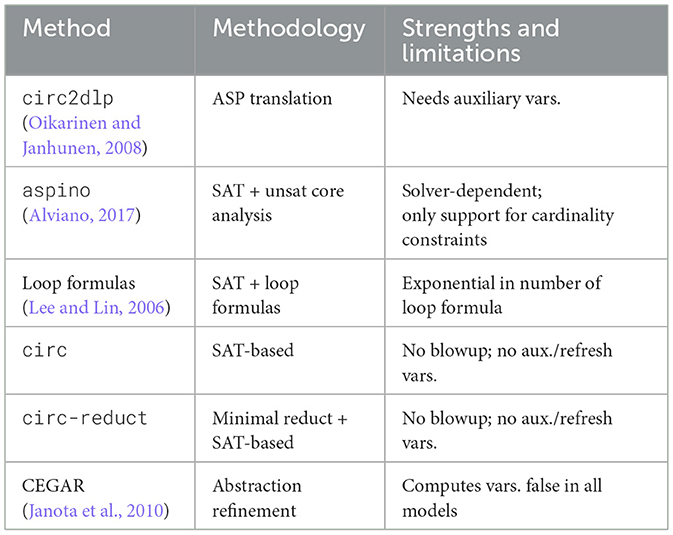
Table 9. Comparison of methods for computing circumscription models.
7 Conclusion and future work
In this study, we introduced the notion of minimal reduct for circumscription and established a new characterization theorem for circumscription based on minimal reduct. We proposed and implemented two algorithms for computing models of circumscription: circ, which operates directly on propositional clause theories, and circ-reduct, which computes with the help of minimal reduct. We further presented the algorithm circ-enum to enumerate circumscription models.
We have evaluated our algorithms circ, circ-reduct and circ-enum on the benchmark model-based circuit diagnosis, random CNFs formulas, and several industrial benchmarks from SAT competitions. The results show that by employing the efficient SAT solver, both circ and circ-reduct are effective and significantly outperform circ2dlp and the solver based on unsatisfiable core analysis aspino. The former translates circumscriptions into disjunctive logic programs under stable model semantics. This study provides new directions for computing circumscription models.
The following issues deserve our further investigation:
• To optimize the model enumeration algorithm circ-enum for circumscription, we aim to draw inspiration from recent advancements in answer set programming (ASP) enumeration techniques (Calimeri et al., 2019; Comploi-Taupe et al., 2023). We plan to incorporate conflict-driven clause learning, backtracking, and heuristic search techniques. Additionally, given the connection between circumscription completion and loop formulas (Lee and Lin, 2006), we will explore how loop formulas can be fully utilized in enumerating circumscription models.
• Given a model of a circumscription, how to establish a justification for the atoms in the model. Similar ideas have been designed from answer set programming with the help of minimal reduct (Wang et al., 2023).
• Note that prioritized circumscription (Lifschitz, 1985) extends parallel circumscription by introducing priorities among minimizing predicates, which allows for the representation of priority-related applications. Given the existence of efficient computational methods for prioritized circumscription (Wakaki and Satoh, 1995, 1997; Chen, 1999; Oikarinen and Janhunen, 2008), we will consider how the notion of minimal reduct can be extended to prioritized circumscription. In particular, since prioritized circumscription can be reduced to the conjunction of multiple parallel circumscriptions, a natural preliminary direction is to apply the proposed minimal reduct approach sequentially to each component. Similarly, nested circumscription, which allows circumscription formulas themselves to appear as components, poses additional challenges. We leave the exploration of extending minimal reduct to nested circumscription as an interesting direction for future work.
• An interesting direction for future work is to extend our algorithms to parallel and distributed frameworks. Currently designed for sequential execution, the algorithms could benefit from parallelization, particularly during minimal reduct computation and model enumeration, which would significantly enhance scalability and efficiency for large-scale instances.
Data availability statement
The datasets presented in this study can be found in online repositories. The names of the repository/repositories and accession number(s) can be found in the article/Supplementary material.
Author contributions
ZX: Software, Writing – original draft, Methodology, Validation. YW: Supervision, Funding acquisition, Conceptualization, Writing – review & editing, Project administration. LY: Writing – review & editing, Validation. RF: Writing – review & editing.
Funding
The author(s) declare that financial support was received for the research and/or publication of this article. This work was supported by the National Natural Science Foundation of China under Grants 62376066 and 61976065.
Conflict of interest
The authors declare that the research was conducted in the absence of any commercial or financial relationships that could be construed as a potential conflict of interest.
Generative AI statement
The author(s) declare that no Gen AI was used in the creation of this manuscript.
Any alternative text (alt text) provided alongside figures in this article has been generated by Frontiers with the support of artificial intelligence and reasonable efforts have been made to ensure accuracy, including review by the authors wherever possible. If you identify any issues, please contact us.
Publisher's note
All claims expressed in this article are solely those of the authors and do not necessarily represent those of their affiliated organizations, or those of the publisher, the editors and the reviewers. Any product that may be evaluated in this article, or claim that may be made by its manufacturer, is not guaranteed or endorsed by the publisher.
Supplementary material
The Supplementary Material for this article can be found online at: https://www.frontiersin.org/articles/10.3389/frai.2025.1614894/full#supplementary-material
Footnotes
1. ^P and Z acts as the minimizing set of atoms and varying set of atoms, respectively.
2. ^https://github.com/shaowei-cai-group/LSTech-Maple
3. ^https://github.com/alviano/aspino
4. ^http://www.tcs.hut.fi/Software/circ2dlp/
5. ^https://github.com/gzu-ai/circ_solver, https://github.com/gzu-ai/circumscription_experiment
6. ^https://github.com/gzu-ai/cnf2any
References
Alviano, M. (2017). Model enumeration in propositional circumscription via unsatisfiable core analysis. Theory Pract. Log. Program. 17, 708–725. doi: 10.1017/S1471068417000278
Alviano, M. (2019). Argumentation reasoning via circumscription with pyglaf. Fundam. Inform. 167, 1–30. doi: 10.3233/FI-2019-1808
Amendola, G., Ricca, F., and Truszczynski, M. (2020). New models for generating hard random boolean formulas and disjunctive logic programs. Artif. Intell. 279:103185. doi: 10.1016/j.artint.2019.103185
Angiulli, F., Ben-Eliyahu-Zohary, R., Fassetti, F., and Palopoli, L. (2022). Graph-based construction of minimal models. Artif. Intell. 313:103754. doi: 10.1016/j.artint.2022.103754
Ben-Eliyahu, R., and Dechter, R. (1993). “On computing minimal models,” in Proceedings of the 11th National Conference on Artificial Intelligence, eds. R. Fikes, W. G. Lehnert (Washington, DC: AAAI Press/The MIT Press), 2–8.
Cadoli, M., Eiter, T., and Gottlob, G. (1992). An efficient method for eliminating varying predicates from a circumscription. Artif. Intell. 54, 397–410. doi: 10.1016/0004-3702(92)90051-X
Cadoli, M., and Lenzerini, M. (1994). The complexity of propositional closed world reasoning and circumscription. J. Comput. Syst. Sci. 48, 255–310. doi: 10.1016/S0022-0000(05)80004-2
Cai, S., and Zhang, X. (2022). “Deep cooperation of CDCL and local search for SAT (extended abstract),” in Proceedings of the Thirty-First International Joint Conference on Artificial Intelligence, IJCAI 2022, Vienna, Austria, 23-29 July 2022, ed. L. D. Raedt, 5274–5278. doi: 10.24963/ijcai.2022/734
Cai, S., Zhang, X., Fleury, M., and Biere, A. (2022). Better decision heuristics in CDCL through local search and target phases. J. Artif. Intell. Res. 74, 1515–1563. doi: 10.1613/jair.1.13666
Calimeri, F., Perri, S., and Zangari, J. (2019). Optimizing answer set computation via heuristic-based decomposition. Theory Pract. Log. Program. 19, 603–628. doi: 10.1017/S1471068419000036
Callewaert, B., Vandevelde, S., and Vennekens, J. (2025). VERUS-LM: a versatile framework for combining LLMs with Symbolic reasoning. CoRR abs/2501.14540. doi: 10.48550/arXiv.2501.14540
Chen, J. (1999). Embedding prioritized circumscription in disjunctive logic programs. J. Exp. Theor. Artif. Intell. 11, 553–563. doi: 10.1080/095281399146427
Comploi-Taupe, R., Friedrich, G., Schekotihin, K., and Weinzierl, A. (2023). Domain-specific heuristics in answer set programming: a declarative non-monotonic approach. J. Artif. Intell. Res. 76, 59–114. doi: 10.1613/jair.1.14091
de Kleer, J., and Konolige, K. (1989). Eliminating the fixed predicates from a circumscription. Artif. Intell. 39, 391–398. doi: 10.1016/0004-3702(89)90018-0
Doherty, P., Lukaszewicz, W., and Szalas, A. (1997). Computing circumscription revisited: a reduction algorithm. J. Autom. Reason. 18, 297–336. doi: 10.1023/A:1005722130532
Dvořák, W., Järvisalo, M., Wallner, J. P., and Woltran, S. (2015). “Cegartix v0.4: a sat-based counter-example guided argumentation reasoning tool,” in International Competition on Computational Models of Argumentation (ICCMA).
Eiter, T., and Gottlob, G. (1993). Propositional circumscription and extended closed-world reasoning are IIp2-complete. Theor. Comput. Sci. 114, 231–245. doi: 10.1016/0304-3975(93)90073-3
Friedrich, G., Stumptner, M., and Wotawa, F. (1999). Model-based diagnosis of hardware designs. Artif. Intell. 111, 3–39. doi: 10.1016/S0004-3702(99)00034-X
Gebser, M., Kaminski, R., and Schaub, T. (2011). Complex optimization in answer set programming. Theory Pract. Log. Program. 11, 821–839. doi: 10.1017/S1471068411000329
Gelfond, M., and Lifschitz, V. (1988). “The stable model semantics for logic programming,” in Logic Programming, Proceedings of the Fifth International Conference and Symposium, Seattle, Washington, USA, August 15-19, 1988 (2 Volumes), eds. R. A. Kowalski, and K. A. Bowen (Seattle, WA: MIT Press), 1070–1080.
Giunchiglia, E., and Maratea, M. (2006). “OPTSAT: a tool for solving SAT related optimization problems,” in Logics in Artificial Intelligence, 10th European Conference, JELIA 2006, volume 4160 of Lecture Notes in Computer Science, eds. M. Fisher, W. van der Hoek, B. Konev, and A. Lisitsa (Liverpool: Springer), 485–489. doi: 10.1007/11853886_43
Hu, X., Jiang, Y., Pedrycz, W., Deng, Z., Gao, J., Tang, Y., et al. (2025). Automated cluster elimination guided by high-density points. IEEE Trans. Cybern. 55, 1717–1730. doi: 10.1109/TCYB.2025.3537108
Janhunen, T., and Oikarinen, E. (2004). “Capturing parallel circumscription with disjunctive logic programs,” in Logics in Artificial Intelligence, 9th European Conference, volume 3229 of Lecture Notes in Computer Science, eds. J. J. Alferes, and J. A. Leite (Lisbon: Springer), 134–146. doi: 10.1007/978-3-540-30227-8_14
Janota, M., Grigore, R., and Marques-Silva, J. (2010). “Counterexample guided abstraction refinement algorithm for propositional circumscription,” in Logics in Artificial Intelligence- 12th European Conference, JELIA, volume 6341 of Lecture Notes in Computer Science, eds. T. Janhunen, and I. Niemelä (Helsinki: Springer), 195–207. doi: 10.1007/978-3-642-15675-5_18
Koshimura, M., Nabeshima, H., Fujita, H., and Hasegawa, R. (2009). “Minimal model generation with respect to an atom set,” in Proceedings of the 7th International Workshop on First-Order Theorem Proving, FTP 2009, Volume 556 of CEUR Workshop Proceedings, Oslo, Norway, eds. N. Peltier, and V. Sofronie-Stokkermans (Aachen: CEUR-WS).
Lee, J., and Lifschitz, V. (2003). “Loop formulas for disjunctive logic programs,” in ICLP, Volume 2916 of Lecture Notes in Computer Science, ed. C. Palamidessi (Cham: Springer), 451–465. doi: 10.1007/978-3-540-24599-5_31
Lee, J., and Lin, F. (2006). Loop formulas for circumscription. Artif. Intell. 170, 160–185. doi: 10.1016/j.artint.2005.09.003
Lifschitz, V. (1985). “Computing circumscription,” in Proceedings of the 9th International Joint Conference on Artificial Intelligence, Volume 1, ed. A. K. Joshi (Los Angeles, CA: Morgan Kaufmann), 121–127.
Lifschitz, V. (1986). “Pointwise circumscription: preliminary report,” in Proceedings of the 5th National Conference on Artificial Intelligence, Volume 1, ed. T. Kehler (Philadelphia, PA: Morgan Kaufmann), 406–410.
Lin, F., and Zhao, Y. (2004). ASSAT: computing answer sets of a logic program by SAT solvers. Artif. Intell. 157, 115–137. doi: 10.1016/j.artint.2004.04.004
McCarthy, J. (1980). Circumscription - a form of non-monotonic reasoning. Artif. Intell. 13, 27–39. doi: 10.1016/0004-3702(80)90011-9
McCarthy, J. (1986). Applications of circumscription to formalizing common-sense knowledge. Artif. Intell. 28, 89–116. doi: 10.1016/0004-3702(86)90032-9
Metodi, A., Stern, R., Kalech, M., and Codish, M. (2014). A novel sat-based approach to model based diagnosis. J. Artif. Intell. Res. 51, 377–411. doi: 10.1613/jair.4503
Niskanen, A., and Järvisalo, M. (2020). “μ-toksia: an efficient abstract argumentation reasoner,” in Proceedings of the 17th International Conference on Principles of Knowledge Representation and Reasoning, KR 2020, eds. D. Calvanese, E. Erdem, and M. Thielscher (Rhodes), 800–804. doi: 10.24963/kr.2020/82
Ogunniye, G., and Kökciyan, N. (2023). A survey on understanding and representing privacy requirements in the internet-of-things. J. Artif. Intell. Res. 76, 163–192. doi: 10.1613/jair.1.14000
Oikarinen, E., and Janhunen, T. (2005). “circ2dlp - translating circumscription into disjunctive logic programming,” in Logic Programming and Nonmonotonic Reasoning, 8th International Conference, Volume 3662 of Lecture Notes in Computer Science, eds. C. Baral, G. Greco, N. Leone, and G. Terracina (Diamante: Springer), 405–409. doi: 10.1007/11546207_36
Oikarinen, E., and Janhunen, T. (2008). “Implementing prioritized circumscription by computing disjunctive stable models,” in Artificial Intelligence: Methodology, Systems, and Applications, 13th International Conference, Volume 5253 of Lecture Notes in Computer Science, eds. D. Dochev, M. Pistore, and P. Traverso (Varna: Springer), 167–180. doi: 10.1007/978-3-540-85776-1_15
Olausson, T., Gu, A., Lipkin, B., Zhang, C., Solar-Lezama, A., Tenenbaum, J., et al. (2023). “LINC: a neurosymbolic approach for logical reasoning by combining language models with first-order logic provers,” in Proceedings of the 2023 Conference on Empirical Methods in Natural Language Processing, eds. H. Bouamor, J. Pino, and K. Bali (Association for Computational Linguistics), 5153–5176. doi: 10.18653/v1/2023.emnlp-main.313
Pan, L., Albalak, A., Wang, X., and Wang, W. (2023). “Logic-LM: empowering large language models with symbolic solvers for faithful logical reasoning,” Findings of the Association for Computational Linguistics: EMNLP 2023, eds. H. Bouamor, J. Pino, and K. Bali (Singapore: Association for Computational Linguistics), 3806–3824. doi: 10.18653/v1/2023.findings-emnlp.248
Przymusinski, T. C. (1989). An algorithm to compute circumscription. Artif. Intell. 38, 49–73. doi: 10.1016/0004-3702(89)90067-2
Rajasekharan, A., Zeng, Y., Padalkar, P., and Gupta, G. (2023). “Reliable natural language understanding with large language models and answer set programming,” in Proceedings 39th International Conference on Logic Programming, ICLP, Volume 385 of EPTCS, eds. E. Pontelli, S. Costantini, C. Dodaro, S. A. Gaggl, R. Calegari, A. S. d'Avila Garcez, et al. (London: Imperial College London), 274–287. doi: 10.4204/EPTCS.385.27
Reiter, R. (1987). A theory of diagnosis from first principles. Artif. Intell. 32, 57–95. doi: 10.1016/0004-3702(87)90062-2
Reiter, R. (1988). “Chapter 12–Nonmonotonic reasoning,” in Exploring Artificial Intelligence, eds. H. E. Shrobe, and the American Association for Artificial Intelligence (Burlington, MA: Morgan Kaufmann), 439–481. doi: 10.1016/B978-0-934613-67-5.50016-2
Ryu, H., Kim, G., Lee, H. S., and Yang, E. (2025). “Divide and translate: compositional first-order logic translation and verification for complex logical reasoning,” in The Thirteenth International Conference on Learning Representations (Singapore: ICLR).
Sakama, C., and Inoue, K. (1995). “Embedding circumscriptive theories in general disjunctive programs,” in Logic Programming and Nonmonotonic Reasoning, Third International Conference, Volume 928 of Lecture Notes in Computer Science, eds. V. W. Marek, and A. Nerode (Lexington, KY: Springer), 344–357. doi: 10.1007/3-540-59487-6_25
Sierra-Santibáñez, J. (2000). “Declarative formalization of strategies for action selection: applications to planning,” in Logics in Artificial Intelligence, European Workshop, JELIA 2000, volume 1919 of Lecture Notes in Computer Science, eds. M. Ojeda-Aciego, I. P. de Guzmán, G. Brewka, and L. M. Pereira (Malaga: Springer), 133–147. doi: 10.1007/3-540-40006-0_10
Stern, R. T., Kalech, M., Feldman, A., and Provan, G. M. (2012). “Exploring the duality in conflict-directed model-based diagnosis,” in Proceedings of the Twenty-Sixth AAAI Conference on Artificial Intelligence, eds. J. Hoffmann, and B. Selman (Toronto, ON: AAAI Press), 828–834. doi: 10.1609/aaai.v26i1.8231
Wakaki, T., and Satoh, K. (1995). “Computing prioritized circumscription by logic programming,” in Logic Programming, Proceedings of the Twelfth International Conference on Logic Programming, ed. L. Sterling (Tokyo: MIT Press), 283–297. doi: 10.7551/mitpress/4298.003.0034
Wakaki, T., and Satoh, K. (1997). “Compiling prioritized circumscription into extended logic programs,” in Proceedings of the Fifteenth International Joint Conference on Artificial Intelligence, Volume 2 (Nagoya: Morgan Kaufmann), 182–189.
Wan, H., Xiao, Z., Yuan, Z., Zhang, H., and Zhang, Y. (2014). “Computing general first-order parallel and prioritized circumscription,” in Proceedings of the Twenty-Eighth AAAI Conference on Artificial Intelligence, eds. C. E. Brodley, and P. Stone (Québec City: AAAI Press), 1105–1111. doi: 10.1609/aaai.v28i1.8860
Wang, Y., Eiter, T., Zhang, Y., and Lin, F. (2023). Witnesses for answer sets of logic programs. ACM Trans. Comput. Logic 24, 1–46. doi: 10.1145/3568955
Wang, Y., Wang, K., Wang, Z., and Zhuang, Z. (2015). “Knowledge forgetting in circumscription: a preliminary report,” in Proceedings of the Twenty-Ninth AAAI Conference on Artificial Intelligence, Volume 29, eds. B. Bonet, and S. Koenig (Frisco, TX: AAAI Press), 1649–1655. doi: 10.1609/aaai.v29i1.9419
Wotawa, F., and Kaufmann, D. (2022). Model-based reasoning using answer set programming. Appl. Intell. 52, 16993–17011. doi: 10.1007/s10489-022-03272-2
Yang, Z., Ishay, A., and Lee, J. (2023). “Coupling large language models with logic programming for robust and general reasoning from text,” in Findings of the Association for Computational Linguistics: ACL 2023, eds. A. Rogers, J. Boyd-Graber, and N. Okazaki (Toronto, ON: Association for Computational Linguistics), 5186–5219. doi: 10.18653/v1/2023.findings-acl.321
Ye, X., Chen, Q., Dillig, I., and Durrett, G. (2023). “SatLM: satisfiability-aided language models using declarative prompting,” in Advances in Neural Information Processing Systems, eds. A. Oh, T. Naumann, A. Globerson, K. Saenko, M. Hardt, and S. Levine (Curran Associates, Inc.), 4554845580. Available online at: https://proceedings.neurips.cc/paper_files/paper/2023/file/8e9c7d4a48bdac81a58f983a64aaf42b-Paper-Conference.pdf
Yuan, L., and Wang, C. H. (1988). “On reducing parallel circumscription,” in Proceedings of the 7th National Conference on Artificial Intelligence, eds. H. E. Shrobe, T. M. Mitchell, and R. G. Smith (Paul, MN: AAAI Press/The MIT Press), 450–454.
Zeng, Y., Rajasekharan, A., Basu, K., Wang, H., Arias, J., Gupta, G., et al. (2024). A reliable common-sense reasoning socialbot built using LLMs and goal-directed ASP. Theory Pract. Log. Program. 24, 606–627. doi: 10.1017/S147106842400022X
Zhang, H., Zhang, Y., Ying, M., and Zhou, Y. (2011). “Translating first-order theories into logic programs,” in IJCAI 2011, Proceedings of the 22nd International Joint Conference on Artificial Intelligence, ed. T. Walsh (Barcelona: IJCAI/AAAI), 1126–1131.
Zhang, J., Fan, R., Tao, H., Jiang, J., and Hou, C. (2023). Constrained clustering with weak label prior. Front. Comput. Sci. 18:183338. doi: 10.1007/s11704-023-3355-7
Keywords: minimal reduct, propositional circumscription, satisfiability, answer set program, model-based diagnosis
Citation: Xie Z, Wang Y, Yang L and Feng R (2025) Minimal reduct for propositional circumscription. Front. Artif. Intell. 8:1614894. doi: 10.3389/frai.2025.1614894
Received: 20 April 2025; Accepted: 13 November 2025;
Published: 10 December 2025.
Edited by:
Francesco Giannini, Scuola Normale Superiore Classe di Scienze, ItalyReviewed by:
Omar A. Alzubi, Al-Balqa Applied University, JordanGiuseppe Mazzotta, University of Calabria, Italy
Yiming Tang, Hefei University of Technology, China
Pan Hu, Shanghai Jiao Tong University, China
Copyright © 2025 Xie, Wang, Yang and Feng. This is an open-access article distributed under the terms of the Creative Commons Attribution License (CC BY). The use, distribution or reproduction in other forums is permitted, provided the original author(s) and the copyright owner(s) are credited and that the original publication in this journal is cited, in accordance with accepted academic practice. No use, distribution or reproduction is permitted which does not comply with these terms.
*Correspondence: Yisong Wang, eXN3YW5nQGd6dS5lZHUuY24=