Segmentation and modeling of large-scale microvascular networks: a survey

Recent advances in three-dimensional microscopy enable imaging of whole-organ microvascular networks in small animals. Since microvasculature plays a crucial role in tissue development and function, its structure may provide diagnostic biomarkers and insight into disease progression. However, the microscopy community currently lacks benchmarks for scalable algorithms to measure these potential biomarkers. While many algorithms exist for segmenting vessel-like structures and extracting their surface features and connectivity, they have not been thoroughly evaluated on modern gigavoxel-scale images. In this paper, we propose a comprehensive yet compact survey of available algorithms. We focus on essential features for microvascular analysis, including extracting vessel surfaces and the network’s associated connectivity. We select a series of algorithms based on popularity and availability and provide a thorough quantitative analysis of their performance on datasets acquired using light sheet fluorescence microscopy (LSFM), knife-edge scanning microscopy (KESM), and X-ray microtomography (µ-CT).

1 Introduction

Microvasculature plays an important role in tissue development and function. While its role is often complex, the shape and structure of microvascular networks are studied in conjunction with disease. Due to imaging constraints, these studies largely focus on the local network structure constrained to a limited field of view or tissue section. Recent advances in three-dimensional microscopy, including light sheet fluorescence microscopy (LSFM) (Kirst et al., 2020), knife-edge scanning microscopy (KESM) (Mayerich et al., 2008), and X-ray microtomography (µ-CT) (Hong et al., 2020; Quintana et al., 2019), overcome this limitation by enabling whole-organ imaging in small animals. However, the microscopy community currently lacks scalable algorithms and benchmarks to quantify microvascular structure at such a large scale.

While many algorithms exist for segmenting vessel-like structures, their scalability on modern whole-organ three-dimensional images has not been rigorously assessed. In addition, segmentation errors can increase disproportionately with volume coverage because acquiring larger volumes introduces trade-offs in SNR, resolution, and sampling anisotropy. This requires more complex algorithms - including pre-processing and machine learning - that are not as scalable as traditional thresholding or segmentation based on localized features (Daetwyler et al., 2019).

In this paper, we propose a comprehensive yet compact survey of available algorithms. We focus on essential features for microvascular analysis, including extracting vessel surfaces and the network’s associated connectivity. Algorithms were selected based on popularity and availability and provide a thorough quantitative analysis of their performance on datasets acquired using emerging techniques.

2 Microvascular models

Microvasculature is a meshwork of capillaries that penetrate tissue to provide nutrients and remove cellular waste. The structure of this mesh changes over time and plays a critical role in tissue function and disease progression. Most current studies are limited to small volumes, primarily characterizing vascular density, along with morphological metrics such as capillary length, radius, and tortuosity (Cassot et al., 2006). These metrics provide fundamental information about the network’s geometric properties and spatial organization. They also serve as the foundation for more advanced analyses, such as quantifying flow dynamics, assessing tissue perfusion, and understanding function. Moreover, downstream pipelines such as computational flow modeling and perfusion simulations can incorporate the segmentations and skeletons to enable quantitative studies of hemodynamics and tissue function (Vidotto et al., 2019).

As image sizes increase, researchers attempt to apply existing metrics at larger scales using software packages like VesselVio (Kirst et al., 2020) or multi-step pipelines such as TubeMap. We expect new metrics and biomarkers to develop over time as larger models are explored. For now, we focus on methods that convert large-scale microvascular images into explicit models that support existing analyses. This leads to two key representations: the microvascular geometry and its skeleton (Figure 1).

Figure 1

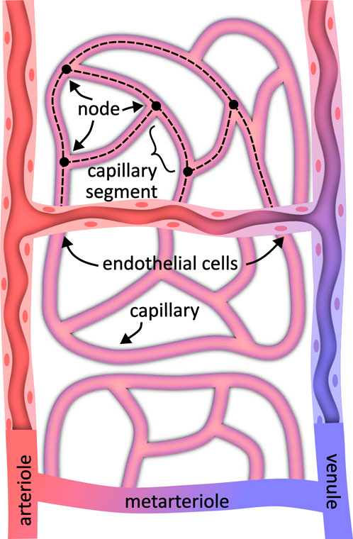
Figure 1. A microvascular model specifies both the geometry representing the surface structure and connectivity in the form of a spatial graph. Depending on the labeling method, the vascular geometry may represent the vessel interior or include endothelial cells lining the vessel and capillary walls. The vessel connectivity generally consists of a graph of vessel centerlines joined at nodes where vessels interconnect.

The geometry of the network represents the vascular surface that separates the region inside from the surrounding tissue. This representation enables the calculation of metrics such as vessel radii, surface area, and volume. The geometry is frequently extracted by identifying these inside/outside regions and then calculating the surface that separates them. Binarization is the first step for resolving the microvascular geometry (Figures 2b,e). These methods rely on separating pixels within the network from the surrounding tissue, providing an implicit representation of the geometry that can be readily converted to an explicit surface mesh.

Figure 2

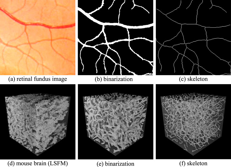
Figure 2. Implicit representations of binarization and skeletonization in 2D and 3D images. Retinal fundus images are shown in 2D (a). The associated binarization (b) indicates pixels that lie inside (white) and outside (black) of the vascular network. The skeletonization (c) shows the vessel paths and points where they connect. The 3D case shows a volumetric visualization of an LSFM image (d) with the associated binarization (e) and centerlines (f).

The network skeleton represents its topology, combining a connectivity graph with vessel centerlines. This representation enables the calculation of metrics such as tortuosity, vessel length, and branching statistics. The skeleton is usually extracted from the geometry using specialized thinning algorithms. Skeletonization is used to extract vessel centerlines (Figures 2c,f) and calculate a connectivity graph. Skeletonization methods frequently rely on an initial binarized volume or surface mesh. However, some techniques, such as tracing, can compute the skeleton directly (Govyadinov et al., 2019).

2.1 Geometry

Vessel geometry can be represented using implicit (voxel-based) or explicit (mesh-based) data structures. In the implicit representation, the vascular network is segmented from surrounding tissue using a three-dimensional voxel grid similar to the original image, with individual voxels labeled as inside or outside vessels. Voxels are convenient for calculating volumes or performing voxel-wise statistical analyses.

Explicit representations, such as polygonal meshes, define vessel surfaces through interconnected vertices and edges. Meshes facilitate calculations of surface area and enable simulations requiring surface geometry. In this survey, all segmentation algorithms produce voxel-based results. We tested two skeletonization algorithms (tagliasacchi and antiga) that require triangular meshes as input, which we produce from segmentation results using the marching cubes algorithm.

This implicit representation can optionally be converted to a surface mesh using algorithms such as marching cubes (Lorensen and Cline, 1998). Measurements are taken across either structure as convenient. For example, surface area can be measured by integrating across a surface mesh, while volume can be measured by adding up the pixels within the network.

2.2 Skeleton

The vascular skeleton is almost always represented explicitly for analysis using connected curves. This explicit representation is fundamentally a connectivity graph, where each node represents a bifurcation and each edge represents a single non-branching vessel segment (Figure 1). The vessel centerlines are curves that can be integrated to calculate features such as length and tortuosity. Algorithms such as depth- and breadth-first searches can also be applied to calculate path lengths and branching characteristics.

In this paper, we evaluate the performance of algorithms for extracting the geometry and connectivity of a microvascular network in large images on imaging methods applicable to whole organs. Most algorithms first binarize the original image using semantic segmentation, using the result as the foundation for medial axis transforms that provide the skeleton (Figure 3).

Figure 3

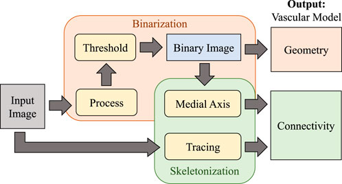
Figure 3. Overview of the vascular modeling pipeline. The input image is first processed (using various filtering or machine learning approaches) and binarized to extract geometry. The medial axis is then calculated to determine network connectivity. Tracing may also be applied directly to the raw image as an alternative approach for skeletonization.

3 Microvascular imaging

Microvascular imaging faces two competing challenges. First, imaging systems must be capable of collecting $\approx$1 mm³ of tissue to characterize network structure, with preferred volume coverages of 1 cm³ for entire rodent organs. Second, the imaging system must resolve microvessels that are less than 10 µm in diameter. Traditional techniques, such as widefield or confocal microscopy, are limited to two-dimensional sections or small volumes. The data in this paper were acquired using recent high-throughput techniques, including (1) X-ray microtomography (µ-CT), (2) light sheet fluorescence microscopy (LSFM), and milling microscopy (Mayerich et al., 2011; Guo et al., 2019).

3.1 Imaging methods

Meeting the criteria for resolution and volume coverage is challenging because microscopes are diffraction-limited and tissue samples are highly scattering. However, recent advances are starting to enable sufficient resolution and volume coverage. This paper considers the following broadly-accessible imaging methods:

X-ray microtomography (µ-CT) is nondestructive and measures the absorbance of X-rays incident on a sample to create three-dimensional images (Ritman, 2004). While µ-CT enables large-volume imaging of whole mouse brains (Hong et al., 2020), its low contrast limits spatial resolution. Recent advances in vascular perfusion compounds such as Vascupaint 2 (MediLumine, Montreal, Quebec, Canada) improve µ-CT resolution to $\approx$20 $\pm$ 4.0 µm, whereas previous contrast agents limited features to $\approx 92\pm$25 µm (Margolis et al., 2024).

Light sheet fluorescence microscopy (LSFM) is characterized by separating illumination and detection. A thin sheet of light illuminates the sample (Hsu et al., 2022), and an orthogonally oriented objective (Figure 4) collects the emitted two-dimensional image using a CCD or CMOS camera. While the penetration depth is traditionally limited by tissue scattering, recent developments in clearing protocols (ex. CUBIC or iDISCO+) (Susaki et al., 2015; Renier et al., 2014) enable large-scale imaging of whole rodent brains. Recent cleared-tissue implementations span a broad range of resolutions. For example, hybrid open-top light sheet systems can achieve lateral resolution of 0.45 µm and axial resolution of 2.9 µm across millimeter-scale volumes (Glaser et al., 2022). When combined with $4\times$ expansion microscopy, LSFM has reached effective resolutions of 375 nm laterally and 750 nm axially in centimeter-scale samples (Glaser et al., 2025). More recently, axially swept LSFM designs have demonstrated nearly isotropic resolution of approximately 300 nm in fixed and cleared tissues (Lin et al., 2025). These gains in resolution typically trade off against imaging volume coverage or acquisition speed, so whole-organ datasets still exhibit significant anisotropy.

Figure 4

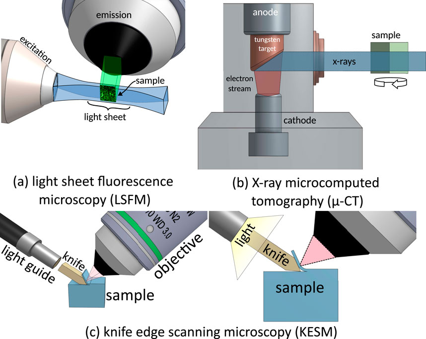
Figure 4. Imaging techniques tested for microvascular reconstruction. (a) Light sheet fluorescence microscopy uses a laser-scanned light sheet to excite fluorophores within a sample plane that are imaged through a high-NA objective. (b) X-ray micro-CT images the sample by rotating it within a transmission X-ray beam. (c) Knife-edge scanning microscopy is a milling-based imaging system that images tissue slices as they are sequentially ablated from a sample.

Milling microscopy removes layers of a sample during the imaging process to expose deeper tissue volumes. Initial experiments used on two-photon microscopy followed by photo-ablation (Tsai et al., 2003), demonstrating that volume constraints could be eliminated by systematically removing tissue. More recent techniques separate tissue sections using physical cutting. Knife-edge scanning microscopy (KESM) (Mayerich et al., 2008; Mayerich et al., 2011) separates a tissue slice from the rest of the block during imaging, while milling with ultraviolet surface excitation (MUSE) performs block-face imaging followed by ablation (Guo et al., 2019).

3.2 Datasets

We evaluated our binarization and skeletonization methods on three datasets representing the modalities described in Section 3.1.

X-ray microtomography (µ-CT) scans of mouse brain (Tg(Slco1c1-BAC-CreER); R26^-lsl-TdTom/+) vascular networks were acquired using a Skyscan 1276 (Bruker, Billerica, MA, United States) at an isotropic sampling rate of 10 µm per voxel. Mice were prepared based on previously published protocols (Suarez et al., 2024). Briefly, the vasculature was perfused with Vascupaint (MediLumine, Product number: MDL-121; Montreal, Quebec, Canada) to provide vascular and microvascular X-ray contrast (Figure 5a).

Figure 5

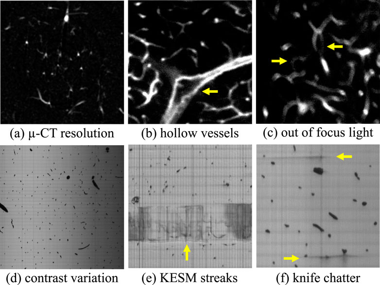
Figure 5. Noise and systematic artifacts that occur in high-throughput imaging techniques. Limitations in resolution (a) reduced the ability to detect small vessels that form connections in the network. Large vessels in LSFM are often hollow (b) because contrast is provided by labeling the vessel wall. Misalignments during imaging can also produce blurry sections (c) that can confound segmentation algorithms. KESM introduces physical artifacts such as variations in illumination across a slice (d) and physical streaks caused by the interaction between the sample and cutting tool (e,f).

Light sheet fluorescence microscopy (LSFM) images of mouse brain microvasculature were acquired using a Cleared Tissue LightSheet (CTLS) Microscopy Workstation XL (3i, Intelligent Imaging Innovations, Denver, CO), equipped with a 30 fps Fusion BT sCMOS camera ($2304\times 2304$ resolution, 6.5 µm pixel size, 95% quantum efficiency, cooled to −50 °C; Hamamatsu Photonics, Japan). Adult C57BL/6N female mice (4.5 months old) were perfused with fluorescently labeled lectin (488 nm; Vector Laboratories, DL-1174-1) as previously described (Ahn et al., 2024), and brains were optically cleared using the iDISCO protocol (Hsu et al., 2022). Imaging was performed using a 1X (0.25 NA) objective and a 488 nm laser at 200 mW power with a 300 ms exposure time. Image stacks were acquired at a 6 µm step size in the Z-direction, with 15% right-side overlap and 50% center tile overlap, making the voxel size $2.0\times 2.0$ $\times$ 6.0 µm. Images were stitched and reconstructed using SlideBook^™ software (Intelligent Imaging Innovations) with the LightSheet module for 3D multipoint acquisition. Raw image files were acquired in 16-bit TIFF format and rescaled to 8-bit using ImageJ for downstream processing. Final voxel spacing was adjusted to 1.0 $\times$ 1.0 $\times$ 0.75 µm using linear interpolation.

Milling microscopy images were acquired using a knife edge scanning microscope KESM at a voxel resolution of $0.6\times 0.7\times 1$ µm, covering a $0.6\times 0.6\times 2$ mm volume. The tissue was acquired from a normal mouse (C57BL/6J) perfused with India ink (Mayerich et al., 2011). The entire dataset is available using the KESM Mouse Brain Atlas (Chung et al., 2011).

Ground truth volumes for training and validation were manually annotated in Slicer (Kikinis et al., 2013). Binarization and skeletonization methods were evaluated on a $200\times 200\times 200$ voxel dataset. The machine learning models were trained on six separate $128\times 128\times 128$ voxel sub-volumes for each dataset (distinct from the $200^3$ sample used for evaluation).

3.3 Noise and artifacts

Each of these imaging modalities introduces sources of noise and other artifacts that challenge segmentation, including:

Resolution limitations are introduced due to both the signal strength and diffraction limit. Standard LSFM is typically anisotropic, with poorer axial than lateral resolution. Recent implementations (Glaser et al., 2022; Lin et al., 2025) can achieve sub-micron isotropic resolution, with trade-offs in speed or volume coverage. µ-CT is primarily limited by SNR to $\approx$20 µm in all three dimensions. Both of these constraints are larger than the diameter of the smallest microvessels (Figure 5a).

Staining and labeling used in LSFM relies on targeting cells in the vessel wall, producing hollow vessels when their diameter is significantly larger than the diffraction limit (Figure 5b). In practice, vascular perfusion with fluorescent compounds like dextran can overcome these artifacts while improving contrast (at the expense of molecular specificity). In that case we would expect images that are more comparable to KESM.

Blurred vessels can occur in LSFM images due to temporary misalignment during long imaging periods (Figure 5c).

Contrast variations are introduced by non-uniform illumination and/or staining in both LSFM and KESM. Contrast is also reduced in LSFM as a function of depth due to scattering.

Machining artifacts introduced by cutting tools in milling microscopy can cause lines (Figure 5e) and streaks (Figure 5f) in individual z-axis slices.

4 Evaluation methodology

We characterize each algorithm’s performance using established metrics and perform an evaluation of adjustable parameters. All algorithms were tested on $200\times 200\times$200 voxel volumes that were manually segmented to create an implicit representation of the geometry and skeleton. If an algorithm requires optimization (ex. U-Net), training is performed on a separate volume acquired from an independent dataset. The same training and validation sets are used for all algorithms.

4.1 Selection criteria

We evaluate a subset of available algorithms based on multiple criteria, prioritizing algorithms used in popular, domain-specific vessel analysis software. This includes Slicer (Kikinis et al., 2013), the Vascular Modeling Toolkit (VMTK) (Izzo et al., 2018), and VesselVio (Bumgarner and Nelson, 2022). Second, we prioritized algorithms with an established open-source implementation that was preferably provided by the authors. We selected representative algorithms from three classes of methods, including: (1) classical thresholding methods, (2) Hessian-based and gradient-based enhancement filters, and (3) deep learning-based semantic segmentation models. We selected skeletonization methods for a range of input data types, including: (1) binarized images, (2) meshes, and (3) point clouds. Our goal is to reflect diverse methodological approaches used for microvascular modeling. This selection process ensures that our evaluation adequately represents current best practices and popular trends in the field, providing a robust benchmark for future developments. Table 1 provides the dates and citations of the proposed algorithms.

Table 1

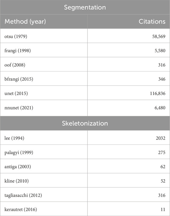
Table 1. Algorithms assessed in this paper for performing binarization (left) and skeletonization (right). The publication date is shown along with their citation count as of this writing.

Otsu’s method was evaluated as a baseline binarization algorithm (otsu3d), and used as the final binarization step as required for other algorithms. Vesselness filters, including both Frangi (frangi) and Beyond Frangi (bfrangi), were included due to their overwhelming popularity for vessel enhancement. Optimally oriented flux (oof) filters were included as a more recent innovation with the open-source implementations provided by the authors. U-Net architectures are extensively used for semantic segmentation in biomedical imaging, so we elected to test a baseline U-Net architecture (unet) while including recent work on self-configured U-Nets (nnunet).

We selected the thinning algorithms by Lee (lee) and Palágyi (palagyi) because of their popularity in skeletonization literature. While the level-set method by Kline (kline) and the confidence accumulation method by Kerautret (kerautret) are not used in existing modeling packages, the authors provide open-source implementations that were tested. We also selected the most recent skeletonization methods available for meshes (tagliasacchi). The selected methods and keywords are provided in Table 2.

Table 2

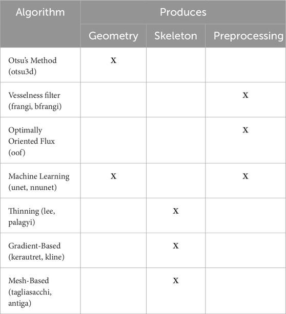
Table 2. Algorithms evaluated in this paper, along with their classes and output data types. Algorithm types are shown in the first column alongside names used to reference the associated results. Remaining columns show the algorithm output (geometry or skeleton). Preprocessing methods such as “vesselness” filters and OOF are used to enhance vessels prior to thresholding with Otsu’s method.

4.2 Geometry metric

Since microvasculature accounts for $\approx$4% of the total tissue volume, we focus on metrics that can accurately characterize unbalanced classifications. The Jaccard similarity index (J) and Dice similarity coefficient (D) are the most common for binarization. The Jaccard index is the normalized volume overlap between the binarization and ground truth:

$J\left(A,B\right)=\frac{\sum \left(A\cap B\right)}{\sum \left(A\cup B\right)}$

The Jaccard index is in the range $J\in [\mathrm{0,1}]$, where $J=0$ indicates no overlap and $J=1$ indicates that the binarization is identical to the ground truth.

We also calculate the precision, emphasizing the accuracy of the positive predictions, and recall, which quantifies the model’s ability to identify true positives. The precision (p) and recall (r) are often combined using the F-score (F), which is both equal to the Dice coefficient and a function of the Jaccard index in the case of binarization:

$F=\frac{2pr}{p+r}=D=\frac{2J}{1+J}$

4.3 Skeleton metric

We adopt the definition of the skeleton as: a set of curves that have identical topology to the geometric surface and are equidistant to the boundary (Wei et al., 2018). We enforce these conditions by manually generating ground truth skeletons based on this definition.

Skeletonization is evaluated using NetMets (Mayerich et al., 2012), which calculates the similarity between two sets of curves $\mathbf{A}$ and $\mathbf{B}$ in 3D space:

$M\left(\mathbf{A},\mathbf{B}\right)=\frac{1}{L}{\displaystyle \sum _{\mathbf{a}\in \mathbf{A}}}\int e^{\frac{d{\left[\mathbf{a}\left(t\right),\mathbf{B}\right]}^2}{2{\sigma }^2}}dt$

where $L$ is the total length of all curves in the set $\mathbf{A}$, $\mathbf{a}(t)$ is a point on the $i$th curve parameterized by $t$, and $\sigma$ is a sensitivity parameter. The function $d(\mathbf{x},\mathbf{B})$ is the distance between a point $\mathbf{x}$ and the closest point in the set of curves $\mathbf{B}$. Given two networks representing the set of curves in the ground truth $\mathbf{G}$ and test case $\mathbf{T}$, the precision (positive predictive value) $P$ and recall (true positive rate) $R$ are calculated:

$P=M\left(\mathbf{T},\mathbf{G}\right)R=M\left(\mathbf{G},\mathbf{T}\right)$

The precision is the percentage of the test skeleton that correctly corresponds to the ground truth, and the recall is the percentage of the ground truth skeleton that is correctly detected in the test case. The sensitivity parameter $\sigma =1$ µm is used for all images.

5 Segmentation algorithms and evaluation

The selected segmentation algorithms largely fall into three groups that largely build on each other: (1) basic thresholding, (2) vessel enhancement and preprocessing, (3) convolutional neural networks.

Thresholding is the most basic approach to binarization, and in many cases an optimal threshold can be calculated automatically. Minimum cross entropy (Li and Tam, 1998), IsoData (Ridler and Calvard, 1978), and Fuzzy thresholding (Huang and Wang, 1995) are popular approaches (Kramer et al., 2022; Huang et al., 2019) that exist in several software packages (Fedorov et al., 2012). The most established algorithm is Otsu’s method, which determines the optimal threshold to separate foreground and background components.

Modern approaches rely on some form of image enhancement that is applied prior to thresholding. This includes filters designed to enhance the contrast of tube-like structures, as well as machine learning to perform semantic segmentation. The methods tested here include vesselness filters (Frangi et al., 1998; Jerman et al., 2016) and optimally oriented flux (OOF) (Law and Chung, 2008).

Convolutional neural networks (CNNs) have taken a prominent role in image segmentation. The U-Net architecture (Ronneberger et al., 2015) and its self-configuring extension, nnU-Net (Isensee et al., 2021), represent the current state-of-the-art in semantic (pixel-level) segmentation. These architectures use a symmetric U-shaped encoder-decoder design (Figure 10) to capture details at multiple scales by processing progressively larger image patches. While machine learning approaches tend to outperform deterministic methods, a significant amount of effort must be applied to annotation and training. As a result, the deterministic approaches are still extensively used in popular software packages.

All methods that require thresholding use Otsu’s method (Otsu, 1979), which computes a threshold $\theta$ that maximizes the between-class variance. Otsu’s method was also tested alone (otsu3d) as a baseline binarization method.

Several preprocessing methods use scale-space filtering (Witkin, 1987) to account for variations in vessel diameter. Scale-space approaches add a discrete dimension to a field (ex. $I(\mathbf{x})\to I(\mathbf{x},s)$) that represents feature sizes. The new dimension is based on a pre-selected set of scale-space parameters $\mathrm{\Sigma }\in [{\sigma }_0,{\sigma }_1,\dots ,{\sigma }_{S-1}]$. The same scale range was used for frangi, ofrangi, and bfrangi. However, the OOF method used slightly smaller values to reach better performance.

5.1 Hessian-based vessel enhancement

The most popular method for enhancing vessels is the Hessian-based approach described by Frangi et al. (1998), originally designed for 2D retinal fundus images. The Hessian matrix is calculated at each point in the image $\mathbf{x}\in {\mathbb{R}}^3$ using finite differences across $S$ scales, creating a field $\mathbf{H}(\mathbf{x},s)\in {\mathbb{R}}^{3\times 3}$. The filter response $V(\mathbf{x})\in \mathbb{R}$ is calculated using the Hessian matrix eigenvalues $(|{\lambda }_1|\le |{\lambda }_2|\le |{\lambda }_3|)$ (Supplementary Algorithm S1). In this study, the method introduced by Yang and Cheng (2014) was also used to accelerate the computations of the Hessian matrix by a factor of two.

The original “vesselness” algorithm (frangi) is outlined in Algorithm 1 and relies on four parameters: tuning parameters $\alpha$, $\beta$, $c$ that target the vessel shape, and a scale parameter $\gamma \approx 2$. The shape parameters are balanced to separate tube-like structures and bifurcations from background pixels (Figure 6). The scalar $\gamma$ was proposed earlier (Lindeberg, 1998) to tune the derivatives used in the Hessian. Attempts to optimize this parameter yield a consistent value of $\gamma =2$ in the literature. We found that this is due to the scale factor ${\sigma }^{\gamma }$ compensating for energy dissipation from the second-order Gaussian scale-space filter. A value of $\gamma =2$ ensures that the most intense response comes from features near the scale-space parameter $\sigma$ (Figure 7).

Figure 6

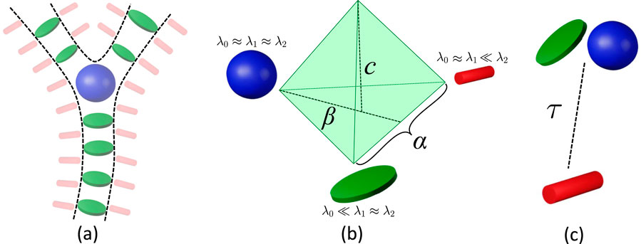
Figure 6. Hessian-based filters emphasize (a) plate-like (green) and blob-like (blue) tensors as vessels and bifurcations, while stick-like (red) tensors emphasize surfaces (including vessel surfaces). (b) The vesselness filter proposed (frangi, ofrangi) uses parameters $\alpha$, $\beta$, and $c$ to target voxels associated with plate-like and blob-like features. $\alpha$ is used to discern between plate-like and line-like structures, $\beta$ emphasizes the deviation from a blob-like structure, and $c$ controls the Frobenius norm of the Hessian matrix and suppresses the noise. (c) bfrangi simplifies these tunable parameters into a single value $\tau$ to differentiate between vessels and background (composed of small and stick-like tensors).

Figure 7

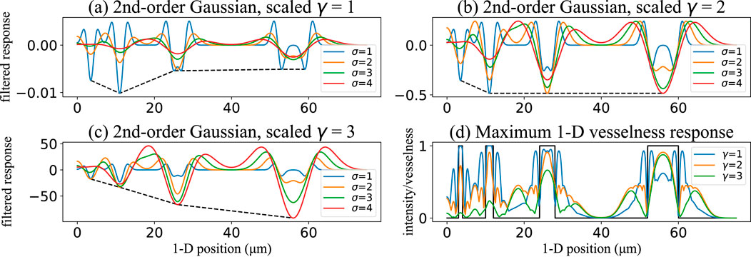
Figure 7. Effect of the scale-normalization exponent $\gamma$ on synthetic one-dimensional vessel cross-sections. The second-order Gaussian derivatives are shown alongside the resulting vesselness response. (a–c) Second derivative responses to a 1D signal convolved with scale-normalized Gaussian second derivatives at multiple scales ($\sigma$ = 1, 2, 3, 4), plotted for different normalization exponents: (a) $\gamma$ = 1, (b) $\gamma$ = 2, and (c) $\gamma$ = 3. (d) Maximum 1D vesselness response (across all scales) for $\gamma$ = 1, 2, and 3. Only $\gamma$ = 2 yields consistent, scale-invariant responses.

Since the parameters in the original algorithm can be challenging to select, we provide two comparisons. First, we examine binarization results based on parameters used in the original paper (frangi), and after parameter optimization (ofrangi) for each dataset using training data. A parallel implementation was used to create sensitivity maps for each parameter (Figure 8). The relationship between parameters for frangi is shown in Figure 6a.

Figure 8

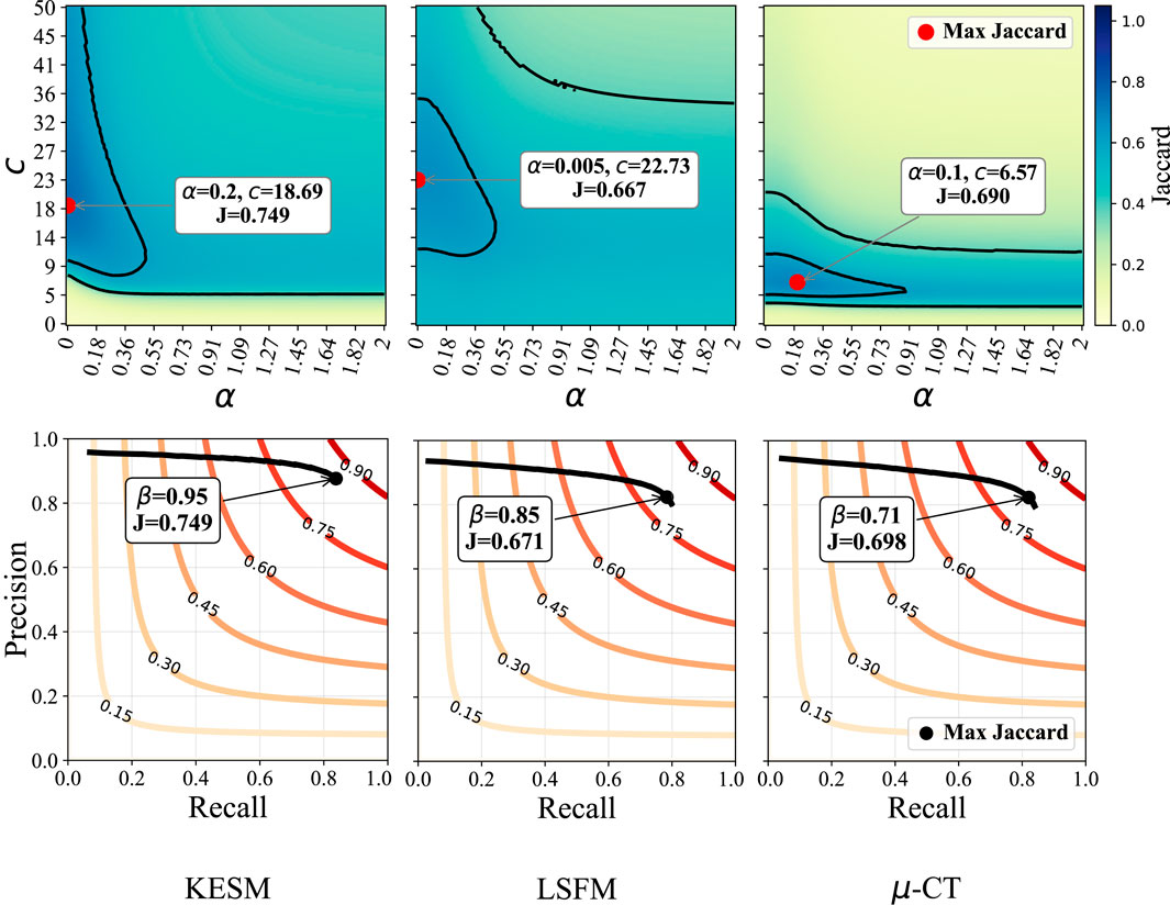
Figure 8. Sensitivity to $\alpha$, $\beta$, and $c$ parameters in frangi method across the three datasets. Top row: Jaccard index (color-mapped) as a function of $\alpha$ and $c$ parameters, with $\beta$ tuning factor held constant (effectively removed, i.e., set to 1). The red dot indicates the parameter combination yielding the maximum Jaccard score for each dataset. Bottom row: Jaccard index (contours) as a function of precision and recall for varying $\beta$ values, with $\alpha$ and $c$ fixed at their optimal values identified in the top row. The black dot marks the point of maximum Jaccard score, and the continuous line shows the score as $\beta$ varies.

A modified implementation of the vesselness framework replaces the parameters with a single normalization term $\tau$ (Jerman et al., 2015). The Beyond Frangi (bfrangi) algorithm (Supplementary Algorithm S2) regularizes the largest eigenvalue at each scale, yielding a more uniform response across vessel cross-sections and intensities. The sensitivity of each dataset to this parameter is illustrated in Figure 9.

Figure 9

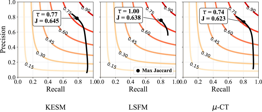
Figure 9. Sensitivity to $\tau$ in the Beyond Frangi method for each dataset. Red curves represent contours where the Jaccard index is constant. Precision-recall curves show the change of both metrics in response to varying $\tau$. The indicated point is the maximum Jaccard index, corresponding to the best parameter for $\tau$ using this metric.

5.2 Optimally oriented flux

The second derivatives within the Hessian are numerically calculated using finite-difference methods, introducing artifacts when features are adjacent. An alternative approach proposes optimally oriented flux (OOF) (Law and Chung, 2010), which relies on first derivatives and integrating gradient information over a spherical region. This applies a hard cut-off that localizes the gradient information used.

Given a point $\mathbf{x}$ in the 3D image $I(\mathbf{x})\in \mathbb{R}$ and a direction vector $\mathit{\rho }$, the gradient flux aligned with $\mathit{\rho }$ is integrated over a sphere $\mathrm{\Omega }$ with radius ${\sigma }_s$ (Figure 10).

$F\left(\mathbf{x},r,\mathit{\rho }\right)={\iint }_{\mathrm{\Omega }}\left(\nabla I\left(\mathbf{x}\right)\cdot \mathit{\rho }\right)\mathit{\rho }\cdot \mathbf{n}dA={\mathit{\rho }}^T\mathbf{Q}\left(\mathbf{x},r\right)\mathit{\rho }$

where $dA$ is the differential area of the sphere and $\mathbf{n}$ is the sphere normal at $\mathbf{x}$. This integral is used to calculate the flux matrix $\mathbf{Q}$. The optimal vessel orientation is the vector $\mathit{\rho }$ that maximizes the outward-oriented flux:

$\underset{\mathit{\rho }}{\max }\left[{\mathit{\rho }}^T\mathbf{Q}\left(\mathbf{x},r\right)\mathit{\rho }\right]$

Our tests used the OOF method available in MATLAB (oof), where the only tunable parameters are the sphere radii $\mathrm{\Sigma }$. In our tests, we use the same $\mathrm{\Sigma }$ values for OOF and scale-space arguments (frangi, ofrangi, bfrangi).

Figure 10

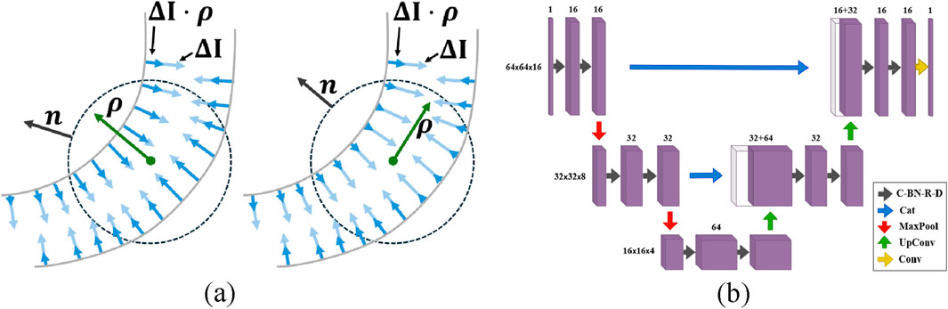
Figure 10. In Optimally Oriented Flux (a), the vessel orientation is determined by maximizing the outward-oriented gradient flux over a spherical region. Diagram of the U-Net architecture (b). The network consists of convolutional layers with batch normalization, ReLU activation, and dropout (C-BN-R-D), concatenation layers (Cat), max-pooling layers (MaxPool), up-convolutional layers (UpConv), and convolutional layers (Conv).

5.3 Convolutional neural networks

The U-Net (unet) architecture uses parallel encoder/decoder paths bridged by skip connections that merge high-resolution features from the encoder into the decoder. The network meta-parameters were determined through iterative trial and error based on validation performance. This U-Net uses 3 × 3 × 3 convolutional layers, ReLU activation, and 2 × 2 × 2 max-pooling layers (Figure 10). The data is divided into smaller volumes, selecting only those with intensities above the global mean to avoid empty or near-empty voxels that reduce training quality (Çiçek et al., 2016). The unet model tested here is trained and tested on these selected volumes using the Focal Tversky loss function (Abraham and Khan, 2019).

The nnU-Net (nnunet) architecture builds on U-Net by overcoming the need for manual meta-parameter tuning. nnU-Net maintains the encoder-decoder structure with skip connections while automatically adapting its architecture and hyperparameters. Like U-Net, it employs 3 × 3 × 3 convolutional layers, ReLU activation, and pooling layers but integrates additional strategies, such as ensemble modeling and deep learning-based boundary enhancement to improve segmentation accuracy (Schott et al., 2023). During training, nnU-Net uses standard loss functions and ensemble modeling, where multiple models are trained and combined. We used the source code provided by the authors¹ for these experiments.

5.4 Geometry results

Our binarization results are shown in Table 3, providing the Jaccard Index, precision, and recall. Otsu’s method (otsu) was tested on raw data and used to select the final threshold for all preprocessing algorithms. The vesselness filter was tested using published parameters in the original paper (frangi) and after optimization of all parameters (ofrangi), while Beyond Frangi (bfrangi) was tested after optimization of $\tau$. Optimally oriented flux (oof) does not require parameter tuning outside of the scale-space parameters used to select sphere radii. Precision-recall curves are provided for the raw output so that the reader can evaluate the results without Otsu’s method (Figure 11). Like most semantic segmentation networks, unet and nnunet integrate binarization into the model and do not require Otsu’s method for thresholding.

Table 3

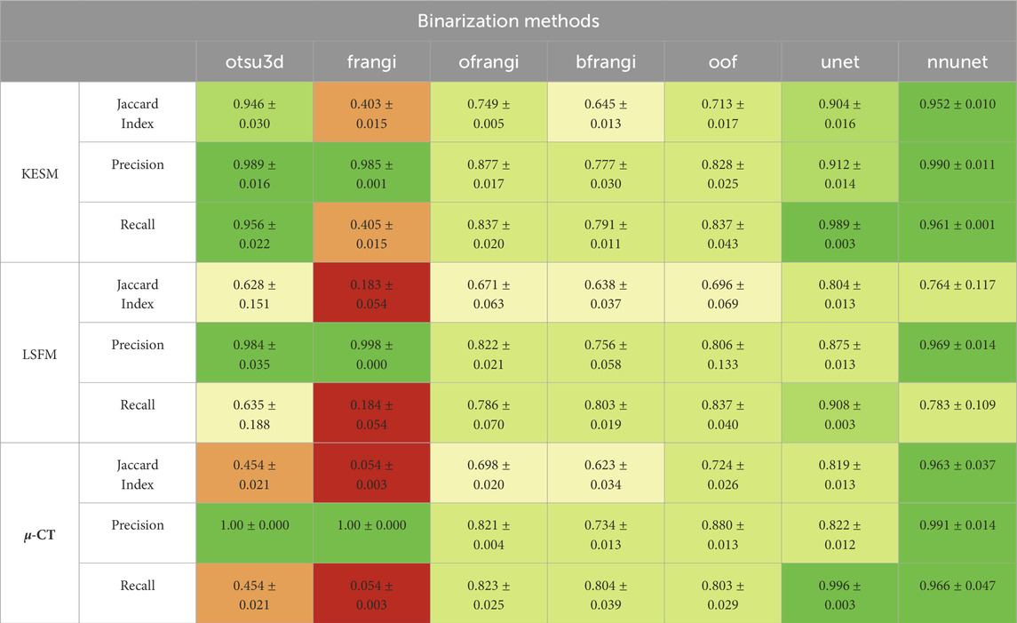
Table 3. Segmentation results showing the Jaccard index, precision, and recall for each binarization algorithm (red = bad, green = good). The original vesselness paper (frangi) recommends 0.5, 0.5, and half of the maximum value of the Hessian norm for $\alpha$, $\beta$, and $c$, respectively. The standard deviation (STD) values are computed as part of a statistical test across three non-overlapping volumes of equal size.

Figure 11

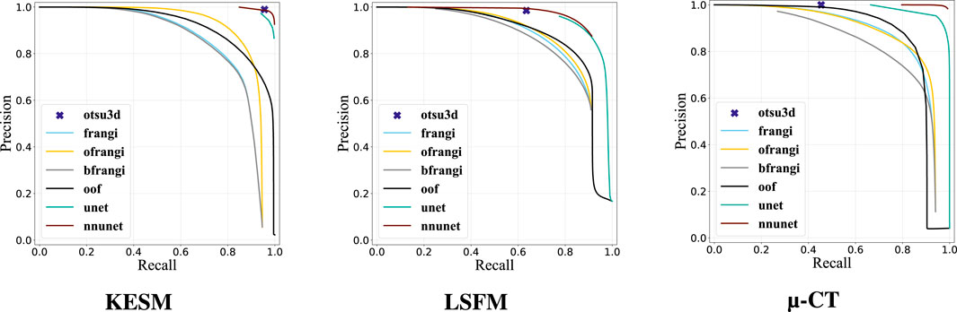
Figure 11. Precision-Recall curve of evaluated segmentation methods.

Raw image sections are provided from each dataset, along with the best corresponding binarization result for each algorithm (Figure 12). Further discussion is provided in Section 7.

Figure 12

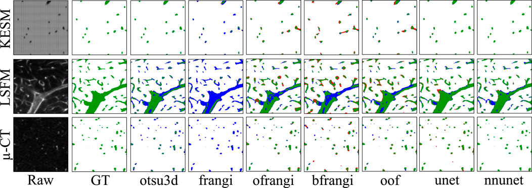
Figure 12. Cross-sections of three-dimensional volumes showing segmentation results for each modality. Green pixels indicate correctly labeled vessels, while white pixels show correctly detected background. Blue indicates undetected vessels (false negatives), while red indicates background pixels that are incorrectly labeled as vessels (false positives). GT indicates the manually annotated ground truth.

6 Skeletonization algorithms and evaluation

The presented skeletonization algorithms require either an initial binary image or a geometric surface. Whenever the vascular surface is required, it is extracted using the marching cubes algorithm from the binarized output.

6.1 Skeletonization

Skeletonization is the method of determining the connected vessel centerlines, usually based on the extracted geometry. A binarized image is used as an input to thinning algorithms, while other approaches calculate the skeleton (or medial axis) from an explicit geometry.

Thinning uses morphological erosion to calculate an implicit representation of the skeleton from a binarized image. Voxels are iteratively removed until a thin single-voxel skeleton remains. The concept was originally proposed in Blum’s grassfire propagation (Blum, 1967), while Tsao and Fu (1981) were the first to introduce a three-dimensional algorithm based on formalized topological and geometric rules. The main concept in erosion-based methods is determining the “simple points” that can be removed without changing the model topology. Thinning algorithms usually differ in how they detect and remove simple points. The most popular method used in current software packages (Fedorov et al., 2012; Bumgarner and Nelson, 2022) is Lee et al. (1994) approach.

Mesh-based medial axis transforms approximate the skeleton from a geometric surface. These include point-sampling methods that leverage ray casting Kerautret et al. (2016) to localize the skeleton. While these methods face challenges when differentiating the “inside” and “outside” of complex shapes (Wei et al., 2018), statistical methods can overcome these problems using vector accumulation maps to probabilistically approximate the skeleton (Kerautret et al., 2016). This can be overcome by directly evolving the geometry towards its centerline using an active contour model (Tagliasacchi et al., 2012).

Another subcategory of mesh-based transforms leverages a Voronoi diagram of the surface (Antiga et al., 2003). The boundaries of the Voronoi cells within vessels can be tracked to extract the medial axis. Despite their precise results, Voronoi-based techniques require careful handling of boundary conditions and specifying seed points to avoid generating spurious branches.

6.2 Thinning

Thinning algorithms reduce an object to a single-voxel-thick centerline while maintaining topology (ex. connectivity, cavities, tunnels). This is accomplished by examining the local neighborhood of each voxel to identify simple points whose deletion preserves topology. These points are iteratively removed until a thinned skeleton remains.

The lee algorithm (Lee et al., 1994) identifies simple points using an octree to recursively subdivide the local neighborhood (Supplementary Algorithm S3). A later approach (Palágyi and Kuba, 1999) uses predefined templates to detect and flag simple points, which is easier to parallelize. Both the sequential lee and parallel palagyi algorithms are parameter-free and take a binarized image as input.

6.3 Gradient-based skeletonization

The Kerautret et al. (2015) algorithm extracts a centerline from a surface mesh by casting rays from each surface point along its normal. The rays are accumulated in a voxel grid where the maximal ridges represent centerlines. The most recent modification (Kerautret et al., 2016) determines an accumulation confidence value for each voxel, where points with higher confidence are more likely to be located on the centerline.

The only required parameter is the accumulation distance $(d_{\mathit{acc}})$ or ray length, which is slightly larger than the maximal radius of the input shape. This value is straightforward to approximate for each volume using the radius of the larger vessels.

The kline algorithm (Kline et al., 2010) calculates a distance field using the fast marching method (FMM), and then internal ridges (maxima) are followed from user-specified seed points. This algorithm assumes that the geometry is a connected tree of tubular structures branching from a single root point. Since microvascular networks do not have a unique root, a large number of seed points are required to comprehensively trace the network.

6.4 Mesh-based skeletonization

The tagliasacchi algorithm (Tagliasacchi et al., 2012) calculates the skeleton from a closed mesh using mean curvature flow (MCF). The medial axis is extracted by moving the mesh along its surface normal proportional to the surface curvature. This iteratively collapses the mesh into a one-dimensional curve (Figure 13). We tested the tagliasacchi method using an implementation provided by StarLab², which requires a watertight manifold mesh and is highly sensitive to mesh boundaries. We forced a watertight mesh at all boundaries and applied the algorithm to each closed mesh component separately.

Figure 13

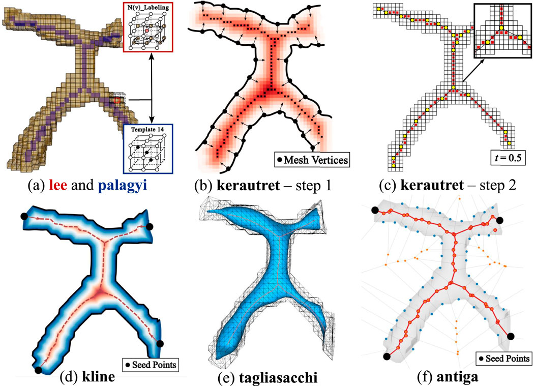
Figure 13. Overview of skeletonization methods. (a) Thinning-based methods: lee applies $N(v)\text{\_}\text{labeling}$ (red), and palagyi applies templates (blue) to detect simple points. (b,c) Kerautret generates a confidence map and extracts the centerline using morphological operations, geodesic segmentation, and FMM. (d) Kline computes a distance field and applies FMM to generate the skeleton through seed points. (e) Tagliasacchi contracts the input mesh iteratively. (f) Antiga constructs a Voronoi diagram to extract centerlines using seed points.

The antiga algorithm (Antiga et al., 2003) builds a Voronoi diagram from point samples of the vascular surface. The intersections of each Voronoi region lie equidistant to the sampled surface, such that medial axis curves can be traced between user-specified seed points. The Delaunay tessellation is calculated from a set of points $P$ that densely samples the vascular surface, which provides the vertices $V$ for the Voronoi diagram. The user specifies a set of seed points $S$ that are connected by selecting points in $V$ that maximize the distance from the vascular surface. This is done by solving an Eikonal equation using the fast sweeping method, ensuring a maximum distance from the boundary surface and providing stability in complex regions like bifurcations. This study uses the implementation of antiga provided in Slicer³. However, the method failed to process seed points or centerlines for messy surfaces created in some LSFM datasets (Table 4).

Table 4

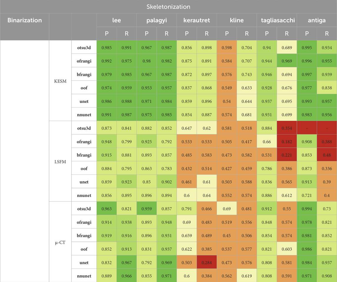
Table 4. Results of centerline extraction on binarization results (left columns: precision, right columns: recall). Thinning was performed using all binarized data for each dataset (see Table 3).

6.5 Skeletonization results

The precision and recall for the proposed skeletonization methods are shown in Table 4. The NetMets algorithm is used to quantify performance using $\sigma =1$ µm. The results are provided using all binarization algorithms as input. The ground truth binarization is also provided as a baseline to demonstrate skeletonization from an “ideal” starting point (Table 5).

Table 5

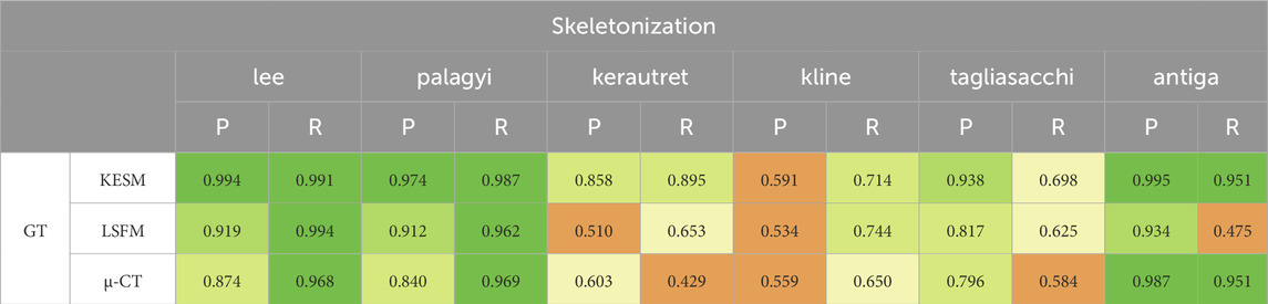
Table 5. Results for skeletonization on the ground truth segmentations.

The lee and palagyi methods achieved the highest F-score across all images, capturing vessel continuity at the cost of adding spurious branches to larger vessels. The antiga method provided the highest precision, however, it identified fewer vessels. The method failed to extract skeletons from binarized results using Otsu’s method due to the excessive number of vertices and edges. Gradient-based methods (kerautret and kline) performed poorly across most images. While kline was designed for vessels, it is poorly suited to microvascular networks since they are not tree-like. The difference in the performance of the kerautret for KESM data also stands out, likely due to the higher resolution of KESM data. This provides (1) a more completely connected mesh and (2) larger distances between adjacent unconnected vessels.

7 Discussion

Machine learning (unet, nnunet) achieved the best consistent performance across all images. This is expected given their established performance on semantic segmentation (Wang et al., 2022). While U-Nets have been extensively explored in two-dimensional images, recent advances that mitigate parameter explosion (Saadatifard et al., 2020) make them more practical in 3D. In our experiments, nnU-Net was run in its 3d_fullres mode, which includes isotropic resampling and intensity normalization. Although effective for KESM and µ-CT, this normalization likely suppressed subtle variations unique to LSFM data, reducing the recall and Jaccard index. It is possible that significantly larger training sets could mitigate these issues.

KESM was generally easier to segment due to its high contrast and spatial resolution. In fact, Otsu’s method (otsu3d) performed similarly to CNNs on KESM data. KESM also exhibits noise and imaging artifacts that are localized to individual slices, potentially making them easier to ignore. The Vesselness algorithms proposed by Frangi et al. (frangi), and later modified by Jerman et al. (bfrangi), are the most popular for enhancing tubular structures. While “out-of-the-box” parameters did not perform well, systematic optimization of these parameters (ofrangi) provided reasonable performance. However, this requires some form of optimization or training that may not provide a benefit over U-Net. If training data is unavailable, optimally oriented flux (oof) provides the best performance.

For skeletonization (Table 4), both lee and palagyi provided consistently good performance. The implementation that we tested for lee⁴ was significantly faster. The antiga algorithm provided the best precision for both KESM and µ-CT data. However, this came at a cost to recall since antiga tended to miss vessel centerlines (Figure 14). It also performed poorly on LSFM data, likely due to the surface complexity. In fact, the algorithm was unable to skeletonize the LSFM data segmented using otsu3d, which exceeded memory limits during the skeletonization process.

Figure 14

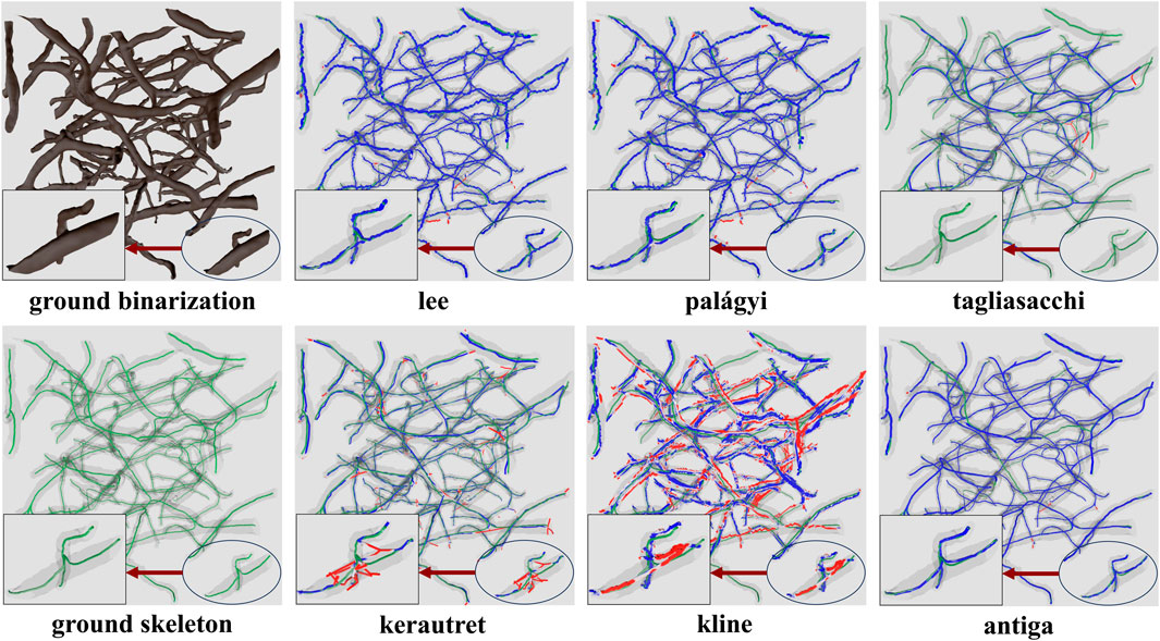
Figure 14. Skeletonization results on the ground truth segmentation of KESM dataset. The ground truth skeleton is colored green in each figure. The skeleton obtained by each method is shown in blue, with false positives marked in red.

One of the more interesting findings was that the most accurate binarization (generally a CNN) did not necessarily provide the best input for skeletonization. For example, otsu3d µ-CT provided better precision than nnunet when used as an input for LSFM and µ-CT. The reduced precision is likely due to consistent mislabeling of internal vessels (Figure 15). All skeletonization algorithms were also tested on ground truth data (Table 5) to demonstrate potential performance given a highly accurate segmentation.

Figure 15

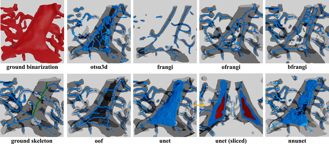
Figure 15. Skeleton extracted using lee using different binarizations. One problem frequently encountered in LSFM is hollow vessels that lead to poor recall in the resulting skeletonization. This is due to regions inside large vessels that are misinterpreted as background. This is most commonly encountered in LSFM because the endothelial cells at the vessel surface are common targets for fluorescent labels. This leads to a variety of incorrect “shells” or “networks” that surround the internal gap. The correct medial axis of the hollow vessel is green in the ground truth image.

8 Conclusion

This work aims to quantify the performance of algorithms for building large-scale microvascular networks. We focus on data from microscopes with the potential for organ-scale vascular imaging (LSFM, KESM, and µ-CT). We tested two classes of algorithms: binarization and skeletonization. These results can be used to reconstruct microvascular surfaces and study network properties. Importantly, the resulting models can feed directly into post-processing frameworks (e.g., CFD-based flow simulations or perfusion analysis) to facilitate functional interpretation and disease modeling (Celaya-Alcala et al., 2021; Zhang et al., 2022). All of the data, annotations, and links to algorithms are available in a public Git repository.⁵

Although KESM and µ-CT images share high contrast and SNR, their disparate voxel resolutions yield very different results: a global threshold such as otsu performs reliably in KESM, yet degrades in µ-CT where learning-based models like nnunet can incorporate local intensity variations to recover performance. It is important to note that this accuracy is quantified with respect to the ground truth and does not account for the reduced resolution of µ-CT: the accuracy of the segmentation does not necessarily reflect the accuracy of the final model. Modality-specific features, such as pixel sizes, ultimately bound the fidelity of the reconstructed vascular model, even when segmentation metrics appear equivalent across algorithms.

If the user can provide annotated training data, they will likely see the best performance using nnunet (Isensee et al., 2021) for binarization, followed by skeletonization with lee (Lee et al., 1994). Users may see an improvement in skeletonization results using antiga, provided the vasculature has a lower total surface area.

If a significant amount of training data is unavailable, the authors recommend oof (Law and Chung, 2008) for binarization, followed by lee for skeletonization. The user may be able to achieve better performance using frangi after significant optimization (ofrangi) (Frangi et al., 1998).

Author contributions

HG: Writing – review and editing, Investigation, Validation, Conceptualization, Software, Methodology, Writing – original draft, Formal Analysis, Visualization, Data curation. AA: Software, Writing – review and editing, Validation. AP: Writing – review and editing, Data curation, Validation. JW: Funding acquisition, Resources, Project administration, Writing – review and editing, Methodology, Data curation. GC: Conceptualization, Methodology, Project administration, Funding acquisition, Writing – original draft, Visualization, Writing – review and editing, Supervision. DM: Writing – review and editing, Formal Analysis, Project administration, Methodology, Supervision, Software, Funding acquisition, Writing – original draft, Conceptualization, Resources, Investigation.

Funding

The author(s) declare that financial support was received for the research and/or publication of this article. This work was supported in part by the University of Virginia Comprehensive Cancer Center (JDW); the National Institutes of Health R01 HL146745 (JDW and DM), R01 HL159159 (JDW), R01 HL173597-01 (DM), and R01DK135870 (DM) and UC2 AR082200 (JDW); and by the National Science Foundation CAREER Award #1943455.

Conflict of interest

DM is a stakeholder in SwiftFront, LLC.

The remaining authors declare that the research was conducted in the absence of any commercial or financial relationships that could be construed as a potential conflict of interest.

Generative AI statement

The author(s) declare that no Generative AI was used in the creation of this manuscript.

Any alternative text (alt text) provided alongside figures in this article has been generated by Frontiers with the support of artificial intelligence and reasonable efforts have been made to ensure accuracy, including review by the authors wherever possible. If you identify any issues, please contact us.

Publisher’s note

All claims expressed in this article are solely those of the authors and do not necessarily represent those of their affiliated organizations, or those of the publisher, the editors and the reviewers. Any product that may be evaluated in this article, or claim that may be made by its manufacturer, is not guaranteed or endorsed by the publisher.

Supplementary material

The Supplementary Material for this article can be found online at: https://www.frontiersin.org/articles/10.3389/fbinf.2025.1645520/full#supplementary-material

Footnotes

¹https://github.com/MIC-DKFZ/nnUNet

²https://github.com/taiya/starlab-mcfskel

³https://www.slicer.org/

⁴skimage.morphology.skeletonize function in the scikit-image Python library.

⁵https://github.com/helia77/MicroVasc-Review

References

Abraham, N., and Khan, N. M. (2019). “A novel focal tversky loss function with improved attention U-Net for lesion segmentation,” in 2019 IEEE 16th International Symposium on Biomedical Imaging (ISBI 2019), Venice, Italy, 08-11 April 2019, 683–687.

Google Scholar

Ahn, T., Largoza, G. E., Younis, J., Dickinson, M. E., Hsu, C.-W., Wythe, J. D., et al. (2024). Protocol for optical, aqueous-based clearing of murine tissues using ez clear. Star. Protoc. 5, 103053. doi:10.1016/j.xpro.2024.103053

PubMed Abstract | CrossRef Full Text | Google Scholar

Antiga, L., Ene-Iordache, B., and Remuzzi, A. (2003). “Centerline computation and geometric analysis of branching tubular surfaces with application to blood vessel modeling,” in Proceedings of the world society for computer graphics (WSCG).

Google Scholar

Blum, H. (1967). “A transformation for extracting new descriptions of shape,” in Models for the perception of speech and visual form, 362–380.

Google Scholar

Bumgarner, J. R., and Nelson, R. J. (2022). Open-source analysis and visualization of segmented vasculature datasets with VesselVio. Cell Rep. Methods 2, 100189. doi:10.1016/j.crmeth.2022.100189

PubMed Abstract | CrossRef Full Text | Google Scholar

Cassot, F., Lauwers, F., Fouard, C., Prohaska, S., and Lauwers-Cances, V. (2006). A novel three-dimensional computer-assisted method for a quantitative study of microvascular networks of the human cerebral cortex. Microcirculation 13, 1–18. doi:10.1080/10739680500383407

PubMed Abstract | CrossRef Full Text | Google Scholar

Celaya-Alcala, J. T., Lee, G. V., Smith, A. F., Li, B., Sakadžić, S., Boas, D. A., et al. (2021). Simulation of oxygen transport and estimation of tissue perfusion in extensive microvascular networks: application to cerebral cortex. J. Cereb. Blood Flow and Metabolism 41, 656–669. doi:10.1177/0271678x20927100

PubMed Abstract | CrossRef Full Text | Google Scholar

Chung, J. R., Sung, C., Mayerich, D., Kwon, J., Miller, D. E., Huffman, T., et al. (2011). Multiscale exploration of mouse brain microstructures using the knife-edge scanning microscope brain atlas. Front. neuroinformatics 5, 29. doi:10.3389/fninf.2011.00029

PubMed Abstract | CrossRef Full Text | Google Scholar

Çiçek, Ö., Abdulkadir, A., Lienkamp, S. S., Brox, T., and Ronneberger, O. (2016). “3d u-net: learning dense volumetric segmentation from sparse annotation,” in Medical Image Computing and Computer-Assisted Intervention–MICCAI 2016: 19th International Conference, Athens, Greece, October 17-21, 2016 (Springer), 424–432.

Google Scholar

Daetwyler, S., Günther, U., Modes, C. D., Harrington, K., and Huisken, J. (2019). Multi-sample spim image acquisition, processing and analysis of vascular growth in zebrafish. Development 146, dev173757. doi:10.1242/dev.173757

PubMed Abstract | CrossRef Full Text | Google Scholar

Fedorov, A., Beichel, R., Kalpathy-Cramer, J., Finet, J., Fillion-Robin, J.-C., Pujol, S., et al. (2012). 3D slicer as an image computing platform for the quantitative imaging network. Magn. Reson. imaging 30, 1323–1341. doi:10.1016/j.mri.2012.05.001

PubMed Abstract | CrossRef Full Text | Google Scholar

Frangi, A. F., Niessen, W. J., Vincken, K. L., and Viergever, M. A. (1998). “Multiscale vessel enhancement filtering,” in Medical image computing and computer-assisted intervention — MICCAI’98. Editors W. M. Wells, A. Colchester, and S. Delp (Berlin, Heidelberg: Springer: Lecture Notes in Computer Science), 130–137. doi:10.1007/BFb0056195

CrossRef Full Text | Google Scholar

Glaser, A. K., Bishop, K. W., Barner, L. A., Susaki, E. A., Kubota, S. I., Gao, G., et al. (2022). A hybrid open-top light-sheet microscope for versatile multi-scale imaging of cleared tissues. Nat. methods 19, 613–619. doi:10.1038/s41592-022-01468-5

PubMed Abstract | CrossRef Full Text | Google Scholar

Glaser, A., Chandrashekar, J., Vasquez, S., Arshadi, C., Javeri, R., Ouellette, N., et al. (2025). Expansion-assisted selective plane illumination microscopy for nanoscale imaging of centimeter-scale tissues. Elife 12, RP91979. doi:10.7554/elife.91979.4

PubMed Abstract | CrossRef Full Text | Google Scholar

Govyadinov, P. A., Womack, T., Eriksen, J. L., Chen, G., and Mayerich, D. (2019). Robust tracing and visualization of heterogeneous microvascular networks. IEEE Trans. Vis. Comput. Graph. 25, 1760–1773. doi:10.1109/TVCG.2018.2818701

PubMed Abstract | CrossRef Full Text | Google Scholar

Guo, J., Artur, C., Eriksen, J. L., and Mayerich, D. (2019). Three-dimensional microscopy by milling with ultraviolet excitation. Sci. Rep. 9, 14578. doi:10.1038/s41598-019-50870-1

PubMed Abstract | CrossRef Full Text | Google Scholar

Hong, S.-H., Herman, A. M., Stephenson, J. M., Wu, T., Bahadur, A. N., Burns, A. R., et al. (2020). Development of barium-based low viscosity contrast agents for micro CT vascular casting: application to 3D visualization of the adult mouse cerebrovasculature. Tech. Rep. 98, 312–324. doi:10.1002/jnr.24539

PubMed Abstract | CrossRef Full Text | Google Scholar

Hsu, C.-W., Cerda III, J., Kirk, J. M., Turner, W. D., Rasmussen, T. L., Suarez, C. P. F., et al. (2022). Ez clear for simple, rapid, and robust mouse whole organ clearing. Elife 11, e77419. doi:10.7554/elife.77419

PubMed Abstract | CrossRef Full Text | Google Scholar

Huang, L.-K., and Wang, M.-J. J. (1995). Image thresholding by minimizing the measures of fuzziness. Pattern Recognit. 28, 41–51. doi:10.1016/0031-3203(94)E0043-K

CrossRef Full Text | Google Scholar

Huang, C., Lowerison, M. R., Lucien, F., Gong, P., Wang, D., Song, P., et al. (2019). Noninvasive contrast-free 3D evaluation of tumor angiogenesis with ultrasensitive ultrasound microvessel imaging. Sci. Rep. 9, 4907. doi:10.1038/s41598-019-41373-0

PubMed Abstract | CrossRef Full Text | Google Scholar

Isensee, F., Jaeger, P. F., Kohl, S. A. A., Petersen, J., and Maier-Hein, K. H. (2021). nnU-Net: a self-configuring method for deep learning-based biomedical image segmentation. Nat. Methods 18, 203–211. doi:10.1038/s41592-020-01008-z

PubMed Abstract | CrossRef Full Text | Google Scholar

Izzo, R., Steinman, D., Manini, S., and Antiga, L. (2018). The vascular modeling toolkit: a python library for the analysis of tubular structures in medical images. J. Open Source Softw. 3, 745. doi:10.21105/joss.00745

CrossRef Full Text | Google Scholar

Jerman, T., Pernus, F., Likar, B., and Spiclin, Z. (2015). Beyond frangi: an improved multiscale vesselness filter. Orlando, Florida, United States, 94132A. doi:10.1117/12.2081147

CrossRef Full Text | Google Scholar

Jerman, T., Pernuš, F., Likar, B., and Špiclin, Ž. (2016). Enhancement of vascular structures in 3d and 2d angiographic images. IEEE Trans. Med. Imaging 35, 2107–2118. doi:10.1109/TMI.2016.2550102

PubMed Abstract | CrossRef Full Text | Google Scholar

Kerautret, B., Krähenbühl, A., Debled-Rennesson, I., and Lachaud, J.-O. (2015). “3d geometric analysis of tubular objects based on surface normal accumulation,” in Image Analysis and Processing—ICIAP 2015: 18th International Conference, Genoa, Italy, September 7-11, 2015 (Springer), 319–331.

Google Scholar

Kerautret, B., Krähenbühl, A., Debled-Rennesson, I., and Lachaud, J.-O. (2016). “Centerline detection on partial mesh scans by confidence vote in accumulation map,” in 2016 23rd International Conference on Pattern Recognition (ICPR), 1376–1381.

Google Scholar

Kikinis, R., Pieper, S. D., and Vosburgh, K. G. (2013). “3d slicer: a platform for subject-specific image analysis, visualization, and clinical support,” in Intraoperative imaging and image-guided therapy (Springer), 277–289.

Google Scholar

Kirst, C., Skriabine, S., Vieites-Prado, A., Topilko, T., Bertin, P., Gerschenfeld, G., et al. (2020). Mapping the fine-scale organization and plasticity of the brain vasculature. Cell180 (04), 780–795. doi:10.1016/j.cell.2020.01.028

PubMed Abstract | CrossRef Full Text | Google Scholar

Kline, T. L., Zamir, M., and Ritman, E. L. (2010). Accuracy of microvascular measurements obtained from Micro-CT images. Ann. Biomed. Eng. 38, 2851–2864. doi:10.1007/s10439-010-0058-7

PubMed Abstract | CrossRef Full Text | Google Scholar

Kramer, B., Corallo, C., van den Heuvel, A., Crawford, J., Olivier, T., Elstak, E., et al. (2022). High-throughput 3D microvessel-on-a-chip model to study defective angiogenesis in systemic sclerosis. Sci. Rep. 12, 16930. doi:10.1038/s41598-022-21468-x

PubMed Abstract | CrossRef Full Text | Google Scholar

Law, M. W. K., and Chung, A. C. S. (2008). “Three dimensional curvilinear structure detection using optimally oriented flux,” in Computer vision – ECCV 2008. Editors D. Forsyth, P. Torr, and A. Zisserman (Berlin, Heidelberg: Springer), 368–382. doi:10.1007/978-3-540-88693-8_27

CrossRef Full Text | Google Scholar

Law, M. W. K., and Chung, A. C. S. (2010). “An oriented flux symmetry based active contour model for three dimensional vessel segmentation,” in Computer vision – ECCV 2010. Editors K. Daniilidis, P. Maragos, and N. Paragios (Berlin, Heidelberg: Springer), 720–734. doi:10.1007/978-3-642-15558-1_52

CrossRef Full Text | Google Scholar

Lee, T. C., Kashyap, R. L., and Chu, C. N. (1994). Building skeleton models via 3-D medial surface axis thinning algorithms. CVGIP Graph. Models Image Process. 56, 462–478. doi:10.1006/cgip.1994.1042

CrossRef Full Text | Google Scholar

Li, C., and Tam, P. (1998). An iterative algorithm for minimum cross entropy thresholding. Pattern Recognit. Lett. 19, 771–776. doi:10.1016/S0167-8655(98)00057-9

CrossRef Full Text | Google Scholar

Lin, J., Marin, Z., Wang, X., Borges, H. M., N’Guetta, P.-E. Y., Luo, X., et al. (2025). Feature-driven whole-tissue imaging with subcellular resolution. bioRxiv. doi:10.1101/2025.01.23.634600

CrossRef Full Text | Google Scholar

Lindeberg, T. (1998). Edge detection and ridge detection with automatic scale selection. Int. J. Comput. Vis. 30, 117–156. doi:10.1023/A:1008097225773

CrossRef Full Text | Google Scholar

Lorensen, W. E., and Cline, H. E. (1998). “Marching cubes: a high resolution 3d surface construction algorithm,” in Seminal graphics: pioneering efforts that shaped the field, 347–353.

Google Scholar

Margolis, R., Merlo, B., Chanthavisay, D., Chavez, C., Trinh, B., and Li, J. (2024). Comparison of micro-CT image enhancement after use of different vascular casting agents. Quantitative Imaging Med. Surg. 14, 2568–2579. doi:10.21037/qims-23-901

PubMed Abstract | CrossRef Full Text | Google Scholar

Mayerich, D., Abbott, L., and McCORMICK, B. (2008). Knife-edge scanning microscopy for imaging and reconstruction of three-dimensional anatomical structures of the mouse brain. J. Microsc. 231, 134–143. doi:10.1111/j.1365-2818.2008.02024.x

PubMed Abstract | CrossRef Full Text | Google Scholar

Mayerich, D., Kwon, J., Sung, C., Abbott, L., Keyser, J., and Choe, Y. (2011). Fast macro-scale transmission imaging of microvascular networks using KESM. Biomed. Opt. Express 2, 2888–2896. doi:10.1364/BOE.2.002888

PubMed Abstract | CrossRef Full Text | Google Scholar

Mayerich, D., Bjornsson, C., Taylor, J., and Roysam, B. (2012). NetMets: software for quantifying and visualizing errors in biological network segmentation. BMC Bioinforma. 13 (Suppl. 8), S7. doi:10.1186/1471-2105-13-S8-S7

PubMed Abstract | CrossRef Full Text | Google Scholar

Otsu, N. (1979). A threshold selection method from gray-level histograms. IEEE Trans. Syst. Man, Cybern. 9, 62–66. doi:10.1109/TSMC.1979.4310076

CrossRef Full Text | Google Scholar

Palágyi, K., and Kuba, A. (1999). A parallel 3D 12-Subiteration thinning algorithm. Graph. Models Image Process. 61, 199–221. doi:10.1006/gmip.1999.0498

CrossRef Full Text | Google Scholar

Quintana, D. D., Lewis, S. E., Anantula, Y., Garcia, J. A., Sarkar, S. N., Cavendish, J. Z., et al. (2019). The cerebral angiome: high resolution microct imaging of the whole brain cerebrovasculature in female and male mice. Neuroimage 202, 116109. doi:10.1016/j.neuroimage.2019.116109

PubMed Abstract | CrossRef Full Text | Google Scholar

Renier, N., Wu, Z., Simon, D. J., Yang, J., Ariel, P., and Tessier-Lavigne, M. (2014). Idisco: a simple, rapid method to immunolabel large tissue samples for volume imaging. Cell 159, 896–910. doi:10.1016/j.cell.2014.10.010

PubMed Abstract | CrossRef Full Text | Google Scholar

Ridler, T. W., and Calvard, S. (1978). Picture thresholding using an iterative selection method. IEEE Trans. Syst. Man, Cybern. 8, 630–632. doi:10.1109/TSMC.1978.4310039

CrossRef Full Text | Google Scholar

Ritman, E. L. (2004). Micro-computed tomography—current status and developments. Annu. Rev. Biomed. Eng. 6, 185–208. doi:10.1146/annurev.bioeng.6.040803.140130

PubMed Abstract | CrossRef Full Text | Google Scholar

Ronneberger, O., Fischer, P., and Brox, T. (2015). U-Net: Convolutional networks for biomedical image segmentation. ArXiv:1505.04597, 234–241. doi:10.1007/978-3-319-24574-4_28

CrossRef Full Text | Google Scholar

Saadatifard, L., Mobiny, A., Govyadinov, P., Van Nguyen, H., and Mayerich, D. (2020). “Cellular/vascular reconstruction using a deep CNN for semantic image preprocessing and explicit segmentation,” in Machine learning for medical image reconstruction. Editors F. Deeba, P. Johnson, T. Würfl, and J. C. Ye (Cham: Springer International Publishing), 134–144. doi:10.1007/978-3-030-61598-7_13

CrossRef Full Text | Google Scholar

Schott, B., Weisman, A. J., Perk, T. G., Roth, A. R., Liu, G., and Jeraj, R. (2023). Comparison of automated full-body bone metastases delineation methods and their corresponding prognostic power. Phys. Med. and Biol. 68, 035011. doi:10.1088/1361-6560/acaf22

PubMed Abstract | CrossRef Full Text | Google Scholar

Suarez, C. P. F., Harb, O. A., Robledo, A., Largoza, G., Ahn, J. J., Alley, E. K., et al. (2024). Mek signaling represents a viable therapeutic vulnerability of kras-driven somatic brain arteriovenous malformations. bioRxiv. doi:10.1101/2024.05.15.594335

CrossRef Full Text | Google Scholar

Susaki, E. A., Tainaka, K., Perrin, D., Yukinaga, H., Kuno, A., and Ueda, H. R. (2015). Advanced cubic protocols for whole-brain and whole-body clearing and imaging. Nat. Protoc. 10, 1709–1727. doi:10.1038/nprot.2015.085

PubMed Abstract | CrossRef Full Text | Google Scholar

Tagliasacchi, A., Alhashim, I., Olson, M., and Zhang, H. (2012). Mean curvature skeletons. Comput. Graph. Forum 31, 1735–1744. doi:10.1111/j.1467-8659.2012.03178.x

CrossRef Full Text | Google Scholar

Tsai, P. S., Friedman, B., Ifarraguerri, A. I., Thompson, B. D., Lev-Ram, V., Schaffer, C. B., et al. (2003). All-optical histology using ultrashort laser pulses. Neuron 39, 27–41. doi:10.1016/S0896-6273(03)00370-2

PubMed Abstract | CrossRef Full Text | Google Scholar

Tsao, Y., and Fu, K. (1981). A parallel thinning algorithm for 3-D pictures. Comput. Graph. Image Process. 17, 315–331. doi:10.1016/0146-664X(81)90011-3

CrossRef Full Text | Google Scholar

Vidotto, E., Koch, T., Koppl, T., Helmig, R., and Wohlmuth, B. (2019). Hybrid models for simulating blood flow in microvascular networks. Multiscale Model. and Simul. 17, 1076–1102. doi:10.1137/18m1228712

CrossRef Full Text | Google Scholar

Wang, R., Lei, T., Cui, R., Zhang, B., Meng, H., and Nandi, A. K. (2022). Medical image segmentation using deep learning: a survey. IET image Process. 16, 1243–1267. doi:10.1049/ipr2.12419

CrossRef Full Text | Google Scholar

Wei, M., Wang, Q., Li, Y., Pang, W.-M., Liang, L., Wang, J., et al. (2018). Centerline extraction of vasculature mesh. IEEE Access 6, 10257–10268. doi:10.1109/ACCESS.2018.2802478

CrossRef Full Text | Google Scholar

Witkin, A. P. (1987). “Scale-space filtering,” in Readings in computer vision (Elsevier), 329–332.

CrossRef Full Text | Google Scholar

Yang, S.-F., and Cheng, C.-H. (2014). Fast computation of Hessian-based enhancement filters for medical images. Comput. Methods Programs Biomed. 116, 215–225. doi:10.1016/j.cmpb.2014.05.002

PubMed Abstract | CrossRef Full Text | Google Scholar

Zhang, Q., Luo, X., Zhou, L., Nguyen, T. D., Prince, M. R., Spincemaille, P., et al. (2022). Fluid mechanics approach to perfusion quantification: vasculature computational fluid dynamics simulation, quantitative transport mapping (qtm) analysis of dynamics contrast enhanced mri, and application in nonalcoholic fatty liver disease classification. IEEE Trans. Biomed. Eng. 70, 980–990. doi:10.1109/tbme.2022.3207057

PubMed Abstract | CrossRef Full Text | Google Scholar