 Bart van Merriënboer
 Jenny Hamer
 Vincent Dumoulin
 Eleni Triantafillou
 Tom Denton
- Google DeepMind, London, United Kingdom
In the context of passive acoustic monitoring (PAM) better models are needed to reliably gain insights from large amounts of raw, unlabeled data. Bioacoustics foundation models, which are general-purpose, adaptable models that can be used for a wide range of downstream tasks, are an effective way to meet this need. Measuring the capabilities of such models is essential for their development, but the design of robust evaluation procedures is a complex process. In this review we discuss a variety of fields that are relevant for the evaluation of bioacoustics models, such as sound event detection, machine learning metrics, and transfer learning (including topics such as few-shot learning and domain generalization). We contextualize these topics using the particularities of bioacoustics data, which is characterized by large amounts of noise, strong class imbalance, and distribution shifts (differences in the data between training and deployment stages). Our hope is that these insights will help to inform the design of evaluation protocols that can more accurately predict the ability of bioacoustics models to be deployed reliably in a wide variety of settings.
1 Introduction
Bioacoustics is an increasingly important and useful tool in conservation (Laiolo, 2010; Dobbs, 2023) with applications in monitoring threatened and endangered species, biodiversity, habitat health, noise pollution, impacts of climate change, and more (Teixeira et al., 2019; Penar et al., 2020). A powerful tool in bioacoustics is passive acoustic monitoring (PAM), which enables large amounts (potentially petabytes worth) of ambient “soundscape” data to be collected cheaply (Gibb et al., 2019). While the collection of this data is inexpensive, transforming it into a format from which insights can be obtained can be costly. Annotating, counting, or otherwise interpreting the data requires expert knowledge and is expensive due to the large scale and the inherent complexity of the data (for instance, due to low signal-to-noise ratio, sparse vocalizations and overlapping vocalizations). While there have been recent advances in computational and automated bioacoustics with the increased adoption of machine learning (ML) techniques (Mcloughlin et al., 2019; Stowell, 2022), there remains a need for more scalable and effective approaches for detecting and classifying various signals within this data (Sugai et al., 2018).
1.1 Foundation models for PAM
Historically, many bioacoustics efforts have focused on building models for specific tasks, e.g., detecting specific species, call types, or individuals in a particular environment, contributing to a collection of specialized and fragmented approaches across the field. This approach is time-consuming, hard to scale, and makes the transfer of knowledge and techniques to different but related tasks and contexts brittle and challenging.
We expect that future work in machine learning for bioacoustics will focus on the development of generalizable models which are easily adaptable to new contexts and problems. This is best illustrated by Ghani et al. (2023), which looks at training linear classifiers on top of embeddings from pretrained global bird species classifiers such as BirdNET (Kahl et al., 2021b) and Google’s Perch model (Hamer et al., 2023). They develop classifiers for bird call-types and dialects, but also species classification models for entire distinct taxonomies such as bats, frogs and marine mammals. They obtain high quality results with as few as four examples per class, demonstrating that these models are highly adaptable. However, more thorough and robust evaluation methods are needed to quantify their utility in the context of other species, PAM, class imbalance and domain shifts, given the complex nature of bioacoustics data.
We also see increasing emphasis on flexible pre-trained models in the broader machine learning context. In other areas, these models are typically trained with copious amounts of unlabeled data, which avoids the cost of data labeling and promises to aid generalization. These large-scale, general-purpose, and adaptable models are loosely referred to as foundation models (Bommasani et al., 2021). Foundation models that can be readily adapted to a wide variety of downstream tasks are starting to be adopted by other fields such as computer vision (Radford et al., 2021), natural language processing (Brown et al., 2020), and more recently, audio (Saeed et al., 2021; Borsos et al., 2023).
In the context of bioacoustics, foundation models could be trained to learn a rich, generalizable representation that may then be adapted to a variety of different tasks—such as detection, classification or source separation applied at the species, individual, or call type level, and even extend to taxa not included at training time. These models could then be modified to perform well in a variety of recording conditions and geographies while being robust to issues such as class imbalance and noisy data.
Unlocking the potential of foundation models for bioacoustics relies on our ability to measure model generalization and adaptability. We find that the literature on this constellation of problems spans multiple branches of research, including bioacoustics, ecology, statistics, and machine learning. The aim of this paper is to bring together insights on many core concerns for those attempting to construct and measure the quality of bioacoustics foundation models.
1.2 Bioacoustics data and challenges
1.2.1 Available bioacoustics data
A varied collection of existing data is available for bioacoustics model training and evaluation. A common distinction is made between focal recordings, which feature a foreground subject, and passive recordings or soundscapes, where subjects may be present in the background and which contain a mix of potentially overlapping species vocalizations. We provide an overview of the different types of datasets and highlight their utility in model development.
1.2.1.1 Large-scale data
Natural sound archives (Ranft, 2004) such as the Macaulay Library of Natural Sounds, the British Library National Sound Archive, and Xeno-Canto (Vellinga and Planqué, 2015) collectively contain hundreds of thousands of recordings adding up to tens of thousands of hours of audio with approximate global coverage. They cover a variety of taxa, but are generally dominated by bird vocalizations. This scale is comparable in size to human speech datasets (Pratap et al., 2020) but smaller than commonly used computer vision datasets (Zhai et al., 2022). The individual recordings generally have lengths ranging from a few seconds to several minutes, are often focal recordings that prominently feature a single animal species vocalizing, and have weak (recording-level) labels. Due to the size, diversity, and geographical coverage of this data (see Figure 1), it is particularly suited for model training.

Figure 1 (Left) The frequency of species in Xeno-Canto recordings is correlated with the estimated abundance of the species (Callaghan et al., 2021) but only weakly so. In general, rare species are relatively over-represented (bottom left). Other potential biases are due to a species vocalizing loudly, like the tawny owl (Strix aluco), or being more common in urban environments in the Western world, like the great tit (Parus major). The San Andres vireo (Vireo caribaeus) is a threatened species endemic to a single Colombian island, but is an outlier because it was recorded extensively by two contributors. On the other hand, several seabirds like the grey-backed tern (Onychoprion lunatus) are very common, but barely represented in Xeno-Canto. (Right) Geographical distribution of Xeno-Canto recordings. Each blue dot represents a single Xeno-Canto recording; bluer regions correspond to geographical areas with higher representation in Xeno-Canto. The Xeno-Canto data has clear geographic biases, for example, towards areas with large human populations (e.g., surrounding Perth in Western Australia) and high-income countries (e.g., Western Europe). The data for these plots was collected by querying the public Xeno-Canto API.
1.2.1.2 Targeted data
There are also smaller, more specialized datasets that share similar format to the large-scale data for specific taxa or species, such as marine mammals (Sayigh et al., 2016), yellowhammer dialects (Diblíková et al., 2019), and bats (Franco et al., 2020). These targeted datasets often contain short focal recordings with clear, high fidelity vocalizations of a single species. This data can be helpful when evaluating specific tasks or settings.
1.2.1.3 Annotated PAM data
The focal recordings found in natural sound archives and specialized datasets are often qualitatively different from the soundscape data collected by PAM projects. This makes these datasets unsuitable for evaluation of models that are to be deployed in PAM projects, as they would provide a poor reflection of the model’s performance in real-world conditions. There are smaller datasets which contain longer recordings that have been more carefully annotated with strong (time-bounded) labels. For example, the BirdCLEF 2021 competition for bird call identification in soundscapes (Kahl et al., 2021a) contains 100 recordings of 10 minutes where all vocalizations have been annotated with bounding boxes in both time and frequency by experts1. Similar datasets exist for mosquitoes (Kiskin et al., 2021) and elephants (Bjorck et al., 2019), to name a couple. Many of these smaller datasets consist of expert annotations on actual PAM data, making them especially valuable for understanding the real-world utility of bioacoustics models in PAM projects and thus excellent candidates for model evaluation. Collectively, however, they have limited coverage and are too small for large-scale, general-purpose model training compared to the larger natural sound archives.
Note that longer recordings, i.e., those that span minutes or even hours, contain long-term temporal structure (Conde et al., 2021). This can be useful in a variety of contexts, for example, if two species are likely to be found in the same location, the vocalization of one species might inform the likelihood of another species vocalizing elsewhere in the recording. Similarly, if an animal vocalizes repeatedly it can help disambiguate ambiguous vocalizations when there are other, clearer vocalizations occurring close in time.
1.2.2 Transitioning to real-world deployment
To ensure that machine learning models are appropriate for the application ecosystem for which they are designed, it is important to minimize the evaluation gap (Hutchinson et al., 2022)—the gap between model performance during evaluation and actual utility during deployment—which involves using tasks, settings, and performance metrics reflective of the final deployment. Determining how to utilize currently available data as described in 1.2.1 for model training and evaluation requires a thoughtful approach. We highlight a variety of challenges and considerations that arise during model development, many of which impact the choice of methodology, metrics, and dimensions of model generalization.
1.2.2.1 Data coverage
There can be significant sampling bias in bioacoustics datasets based on geography, species abundance and loudness of vocalizations, to name a few factors. (Figure 1). In many cases, a target vocalization in a deployment may not be present at all in the training data, requiring models with capacity for out-of-distribution generalization, such as few-shot or transfer learning. In these instances, using heldout data from the training set to create a test set (i.e., evaluating on a new recording for species present in the training data) will not provide information about the model’s (in)ability to detect species not present in the training data.
1.2.2.2 Dataset shifts
Depending on the datasets used during training and test time, data and/or label distributions can differ significantly—this difference is known as dataset shift (Quinonero-Candela et al., 2008; Moreno-Torres et al., 2012). Differences between training and deployment conditions introduce various forms of distribution shift which present model generalization challenges. For instance, a trained bird vocalization detector may be deployed in a new geographical area with different environmental conditions, species population levels, and vocalization types. Furthermore, almost all bird vocalization datasets have significant label imbalance: bird species abundances in Xeno-Canto recordings are not necessarily representative of the true estimated population in nature (Figure 2), and different region-specific bird vocalization datasets deviate significantly from Xeno-Canto in bird species population (Table 1).
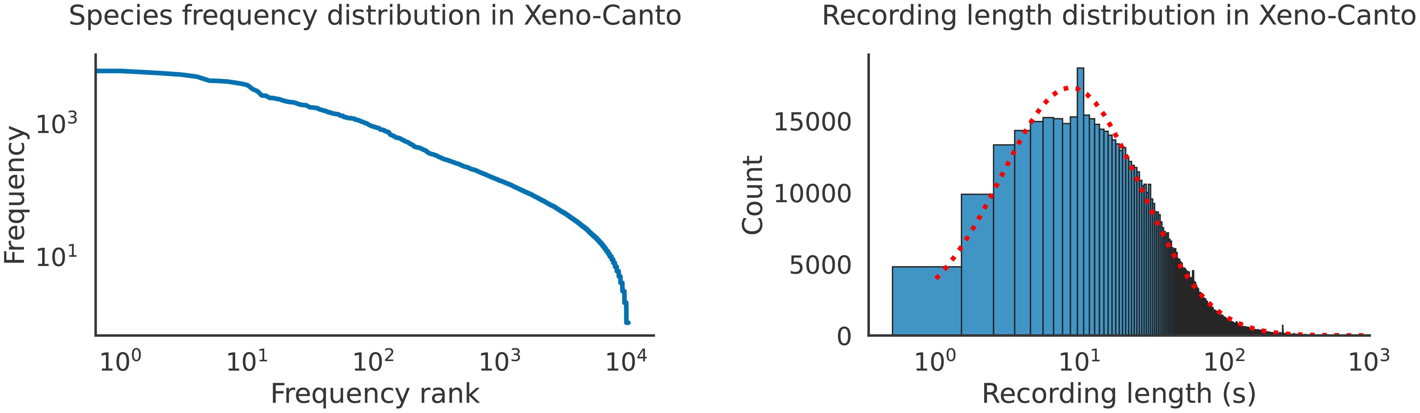
Figure 2 Both the foreground species frequency distribution and the recording length in Xeno-Canto recordings are unbalanced. The recording length distribution is approximately log-normal, with an outlier at 10 s. Data was retrieved from the public Xeno-Canto API.
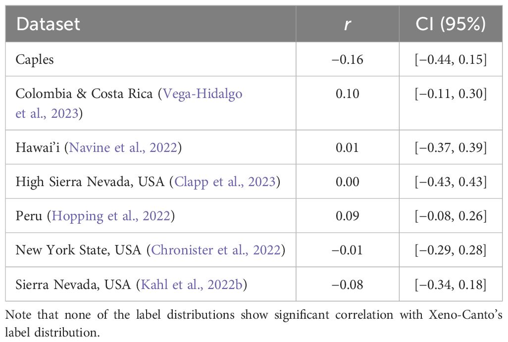
Table 1 Pearson correlation coefficient (r) between the label frequency distribution of a variety of avian soundscape datasets and Xeno-Canto, along with the 95% confidence interval.
Recording length can vary between two datasets, and sometimes within a given dataset (Figure 2, right); variability in temporal structure and context, particularly between training and evaluation data, can contribute to weak generalization.
1.2.2.3 Deployment condition
Differences in deployment condition of a dataset are important to consider. Depending on where and how the dataset was collected, there may be a various sources and concentrations of environmental noise. The microphone used to collect bioacoustic data can impact sound quality, frequency response, polar pattern, etc., while digitization choices, such as compression and sampling rate, can impact its resolution. Focal recordings are typically directional and focused on a given foreground subject, whereas passive recordings might have been recorded with an omnidirectional microphone and contain a multitude of vocalizations and environmental noises. Differences in setting can substantially impact the signal-to-noise ratio in a given recording and the difficulty of detecting a vocalization. Similarly, soundscape datasets commonly include overlapping vocalizations from different species or different individuals, which are often more challenging for a model to learn to disentangle and detect.
1.2.2.4 Annotation and labeling
Annotation quality and fidelity varies greatly depending on the source of the data. The majority of data on Xeno-Canto, a global citizen-science platform for sharing wildlife sounds, features recordings of birds that have been annotated by bird and nature enthusiasts with a wide range of expertise. While many recordings feature reliable labels for focal species, background labels may or may not exist and can be considered weak in that they may be missing even if a species is vocalizing. This can occur with focal recordings but particularly with soundscape recordings where events with lower signal-to-noise ratio might be missed or ignored by annotators.
When dataset attributes such as these differ between training and evaluation data during model development, there can be substantial and potentially confounding negative impacts to the model’s performance when deployed.
1.3 Robustness and practical utility
When designing evaluation protocols for bioacoustics models, it is important to take into account the characteristics of bioacoustics data and challenges that these introduce (Section 1.2). For example, if a model consistently fails to predict rare and endangered species it might have limited utility in practice. However, a naive evaluation protocol that measures average performance across all vocalizations using highly class-imbalanced data might not identify this shortcoming.
Furthermore, testing a model’s ability to handle dataset shifts is important in practice because models are often used to evaluate how species presence relates to environmental covariates. For example, a large PAM deployment will cover many sites, and we want to understand how occupancy and abundance varies across time, elevation, human interventions, and so on. If the model’s performance degrades significantly as a function of these covariates (e.g., it is less likely to detect species at certain sites or times of day) it becomes increasingly likely to draw spurious conclusions from the data. Well-designed evaluation procedures should be able to identify such issues.
1.4 Survey overview
To support minimizing the evaluation gap for foundation models, we require a paradigm shift away from traditional evaluation methods, which usually involve reporting the performance of the model on a uniformly random held-out test set. Instead, a stronger emphasis must be put on robustness, e.g., generalization to new domains, label shift, and adaptation, including few-shot or zero-shot capabilities (Bommasani et al., 2021). These considerations are particularly important for bioacoustics, given that the field naturally deals with large dataset shifts while having comparatively little labeled data available for training.
There is no one-size-fits-all evaluation protocol for foundation models, but we will review several relevant fields to inform the design of evaluation protocols for bioacoustics foundation models. Firstly, we will consider the task of sound event detection and the different evaluation paradigms (Section 2). Then we will review a variety of metrics such as ROC AUC and average precision (Section 3). Finally, we will look at ways to evaluate a model’s ability to generalize by reviewing how evaluation is done in fields like domain generalization, domain adaptation, transfer learning, and few-shot learning (Section 4). We will discuss how these different methods have been applied in bioacoustics in the past (Section 5).
2 Sound event detection
A wide variety of machine learning tasks can be relevant in bioacoustics, notably: binary, single- and multi-label classification, detection, counting and source separation. Motivated by the use case of PAM, we will describe the task of sound event detection (SED; Mesaros et al., 2016, Mesaros et al., 2021) in more detail here. SED is the task of detecting and classifying acoustic events within a longer recording (e.g., of several minutes or hours). Common questions in PAM deployments include whether a specific species is present, which set of species is present in the data, or how often a certain species vocalizes. All of these questions can be answered by the results of a SED task.
A sound event is defined as a triplet of start time, end time, and label. Given an annotated dataset of sound events, there are two common ways of using these annotations in a SED evaluation setup (Figure 3; Mesaros et al., 2021): segment-based and event-based.
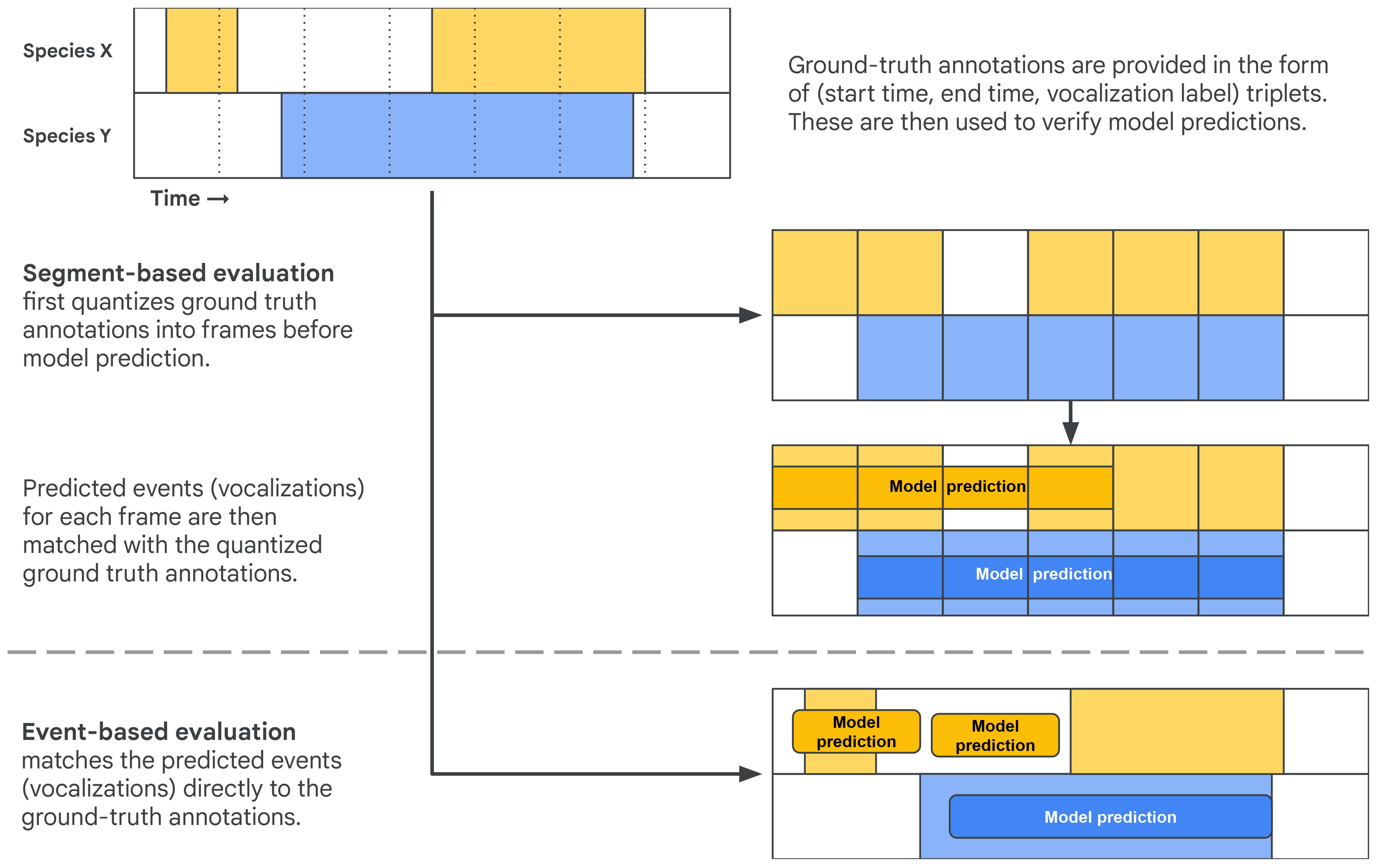
Figure 3 A comparison of event-based (top) and segment-based (bottom) evaluation of sound event detection models, in this case tackling a species-level vocalization detection task. Both operate over a given span of recording containing vocalizations of species X and species Y.
2.1 Segment-based evaluation
The first approach is segment-based evaluation, which involves comparing the ground truth labels and model outputs on a fixed temporal grid: The audio will be divided into frames (windows), which can optionally overlap with neighboring frames. These frames will be assigned labels from the ground truth annotations based on some criterion. Often a simple criterion is used: If the frame has any overlap with a ground truth annotation, it inherits the class label. Figure 3 exemplifies this strategy: the events for two classes are discretized onto a fixed temporal grid, and each frame in the grid is assigned the labels of the events with which it overlaps in time (Figure 3, top).
In the context of evaluation, the resulting task (Figure 3, bottom) is often evaluated in one of the following ways:
● A series of binary classification tasks: for each class, each frame is predicted as having signal or no signal for that class;
● A series of multi-label classification tasks: each frame is predicted as having signal for one, many, or none of the classes (the latter reflecting the detection aspect of SED); or
● When ranking the frames by their likelihood of containing an event of a given class, a series of retrieval tasks (Schütze et al., 2008) where each class is a query and each frame is a document.
These perspectives can inform which evaluation metrics to use (e.g., binary classification metrics such as F1-scores or retrieval metrics such as average precision). But note that SED as a task differs from binary/multi-label classification and retrieval in that in SED the model is allowed to see the entire recording (i.e., all frames) before making its predictions and therefore it does not treat each frame independently.
In practice, however, it is often computationally prohibitive for a model to process the full recording (which can be several minutes or hours long). So in many cases models use a more limited context to make predictions for each frame, and in some cases models do in fact choose to make predictions for each frame independently.
Other things to note are:
● The resolution of the temporal grid is important. If the goal is to evaluate a model’s ability to retrieve segments of the recording to present to a user, then a resolution of several seconds is reasonable. If the goal of the model is to, e.g., count the number of vocalizations or to filter the detected signal out of the recording, then a higher resolution might be more appropriate. It is also important to consider the nature of the events to be detected (e.g., bird vocalizations are generally limited to a few seconds whereas whale songs contain phrases that are several minutes long).
● The naive heuristic for assigning labels to segments can lead to edge cases in which a segment is assigned a label of an event that only overlaps with the segment for a very short period of time. This can be problematic, particularly for models which do not utilize the temporal information across frames.
2.2 Event-based evaluation
The second approach is called event-based evaluation and compares the annotated event instance directly to the predicted events from the model (Figure 3, bottom left). Unlike segment-based evaluation, event-based evaluation does not require deciding on a fixed temporal grid and assigning labels to frames; instead it requires a criterion for deciding whether a predicted event matches a ground truth annotation. This criterion must ideally be robust to varying durations in ground truth annotations and uncertainty in their onset and offset time.
A common way of matching predicted events to the ground truth is by comparing the start and end time of the event while allowing for a small difference, which is referred to as the collar (Figure 4, left; Mesaros et al., 2021). An alternative approach is to use intersection over union (IoU) with a specific threshold (Figure 4, right). Note that IoU is a relative measure, i.e., a larger difference between starting and ending times is allowed for ground truth annotations with longer durations. This is why the first prediction matches the ground truth annotation in Figure 4’s right example whereas the second prediction does not.
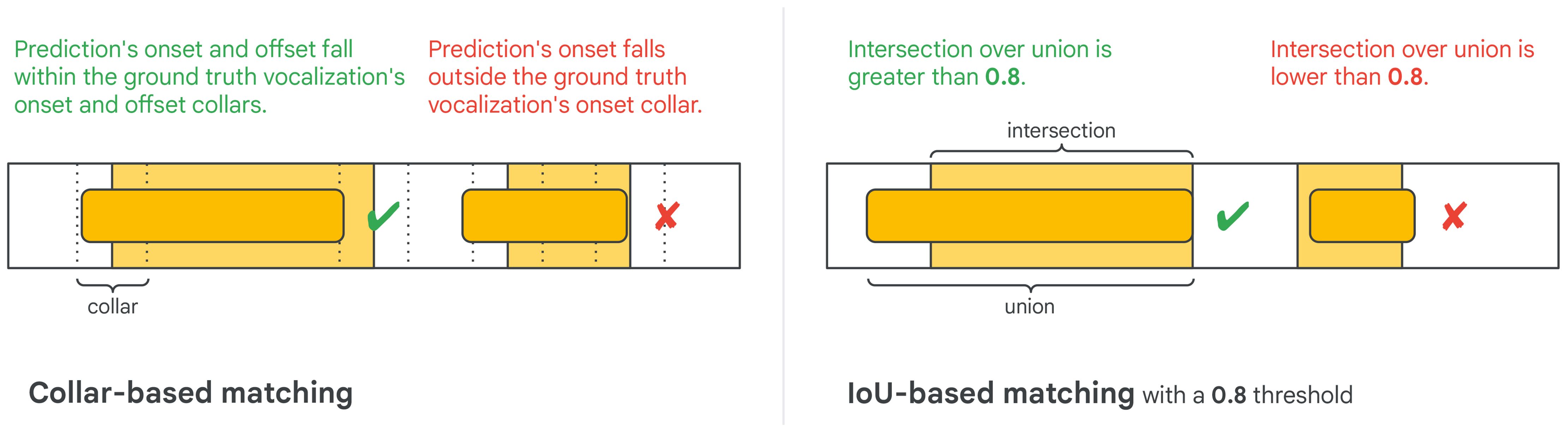
Figure 4 Collar-based and IoU-based event matching criteria.
Figure 4’s predictions each naturally align with exactly one ground truth annotation, but this is not always the case: there could be multiple overlapping ground truth annotations (e.g., if the dataset is densely annotated), or the model could make multiple overlapping predictions. Under either collar-based or IoU-based matching criteria this could result in many-to-one or one-to-many pairings between predictions and ground-truth annotations (Figure 5, top). Counting all matches when multiple predictions are matched to a single ground truth annotation is problematic, since it could allow a model to artificially inflate its number of true positives by duplicating predictions. Counting all matches when a single prediction is matched to multiple ground truth annotations could be problematic or not depending on the intended application (e.g., it is problematic when counting individuals but not when detecting presence). A systematic way of handling these corner cases is to enforce a one-to-one mapping between predictions and ground truth annotations and handling leftover predictions and ground truth annotations in a way that is appropriate for the evaluated application. The one-to-one mapping can be obtained by solving a linear (unbalanced) assignment problem (i.e., bipartite graph matching) using the difference between start and end times or the IoU values as scores (Figure 5, bottom; Stewart et al., 2016).
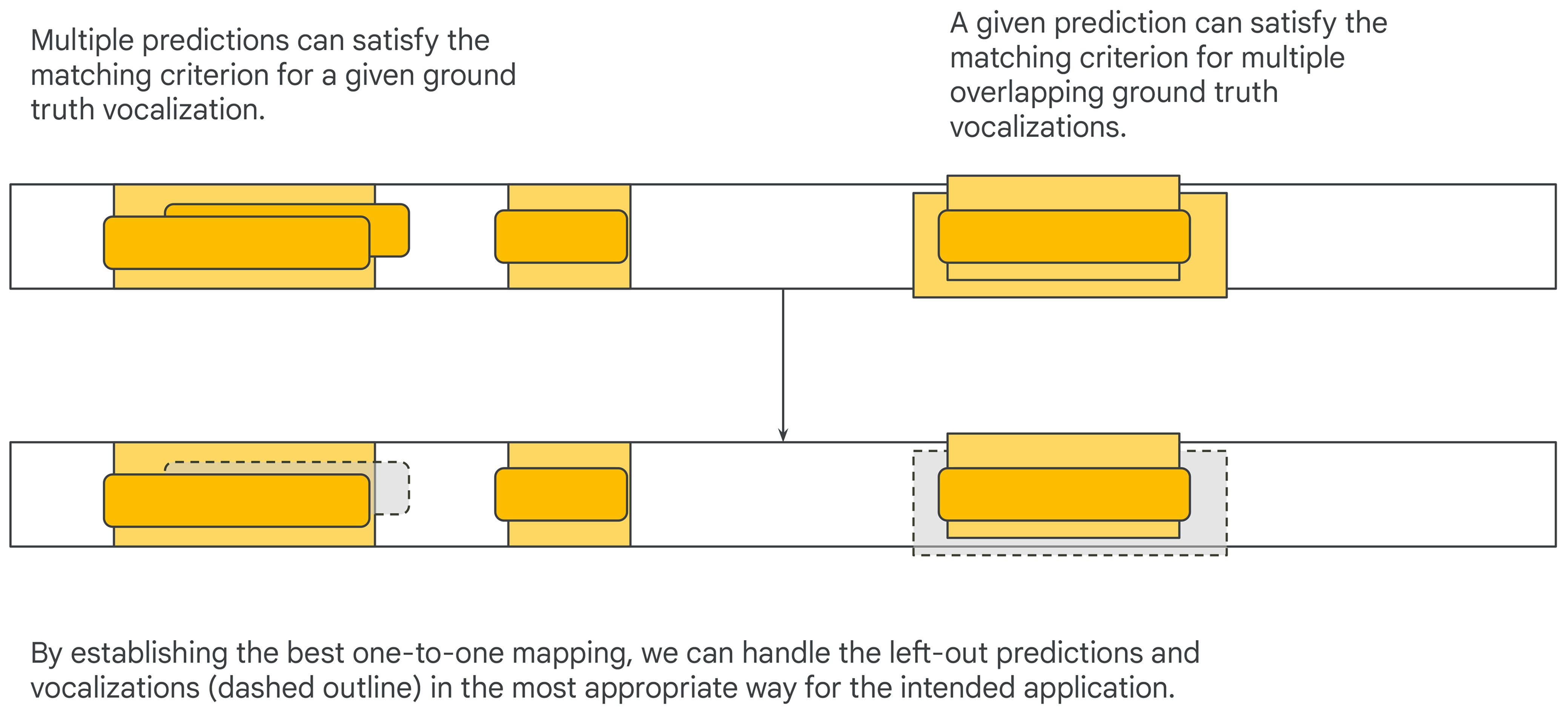
Figure 5 Edge cases to consider are when a predicted event matches multiple ground truth annotations and vice versa.
In other cases it is unclear whether an event should be labeled as a single long event or two shorter consecutive events in the ground truth. If the model predicts a single event when annotators split the event into two consecutive events or vice versa, the collar-based or IoU-based matching criteria could reject the prediction(s) (Figure 6). These concerns are uncommon in traditional fields such as keyword spotting, but are more realistic in bioacoustics. To be robust to these annotation choices, a single prediction can be made to match multiple ground truth annotations and vice versa (Bilen et al., 2020; Ebbers et al., 2022)2. Similarly to regular matching, either an absolute measure can be used (e.g., a ground truth annotation is considered matched if it fully intersects with predictions that had a collar added) or a relative one (e.g., a certain fraction of the ground truth annotation intersects with predictions).

Figure 6 Edge cases to consider are when there is ambiguity in the number of consecutive events.
When there are multiple classes to detect it is possible that the model correctly detects an event but confuses one class for another (cross-triggers; Bilen et al., 2020). Distinguishing between detection failures and cross-triggers may provide valuable insights into model performance, but is relatively under-explored.
3 Metrics
In segment-based evaluation the predictions can readily be classified as true and false positives and negatives, and the full range of binary classification metrics are at our disposal.
For event-based evaluation, the situation is more nuanced, and depends on the matching of model-predicted events to ground-truth annotations. When an event predicted by the model is matched to a ground-truth event, we consider it a true positive (TP). Unmatched predictions are considered false positives (FP), and any remaining unmatched ground-truth annotated events are considered false negatives (FN). Note that none of these three circumstances corresponds to true negatives (TN). Hence, only metrics that do not rely on true negatives (Cao et al., 2020, Table 2) can readily be computed. Examples of such metrics are precision , recall , and the F1-score (the harmonic mean of precision and recall). The false positive rate is an example of a metric that cannot be easily calculated for event-based evaluation.
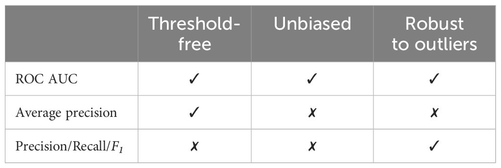
Table 2 An informal summary of metric characteristics.
3.1 Threshold-free metrics
Metrics such as precision and recall are a function of the model’s operating point (decision threshold). This means that our understanding of the model’s performance is dependent on the choice of threshold. Choosing an arbitrary threshold risks underestimating overall model quality and can hinder model comparison. But choosing an appropriate threshold for each model can be a complex process. The optimal choice of threshold likely depends on the downstream application (e.g., often high recall is preferred for detection of rare species, but high precision is preferable when monitoring a wide range of species) and can even be different for different species or deployments. We can avoid the need for tuning thresholds when evaluating models by using threshold-free metrics.
One common way to remove dependence on a particular choice of threshold is to define a metric by integrating over all possible values of the threshold: This gives rise to area-under-the-curve (AUC) statistics. For AUC metrics, a pair of metrics, , are plotted as a function of the threshold, t, defining a parametric curve, . When the true and false positive rate (sensitivity and fall-out) are plotted this is known as the receiver operating characteristic (ROC) curve. Another common curve is the precision-recall (PR) curve. Sometimes the ROC curve is drawn on a logistic scale, in which case it is known as the detection error tradeoff (DET) graph (Martin et al., 1997). Other curves such as the MCC-F1 curve can also be of interest (Cao et al., 2020), which combines MCC and F1, two threshold-free metrics. The Matthews correlation coefficient (MCC) is also known as the phi coefficient in statistics, and is equal to the Pearson correlation coefficient estimated for two binary variables.
For the PR and ROC curves the areas under the curves are known as the average precision and ROC AUC scores respectively (alternatively, AUPR and AUROC). ROC AUC is commonly used in sound event detection. Average precision is often recommended in information retrieval because it emphasizes the model’s positive predictions only (Saito and Rehmsmeier, 2015; Sofaer et al., 2019). This behavior of average precision is shown in Figure 7. The Concentrated ROC (CROC) curve is a monotonic scaling of the ROC curves which emphasizes the early-retrieval performance of the classifier and is used in similar situations as average precision (Swamidass et al., 2010).
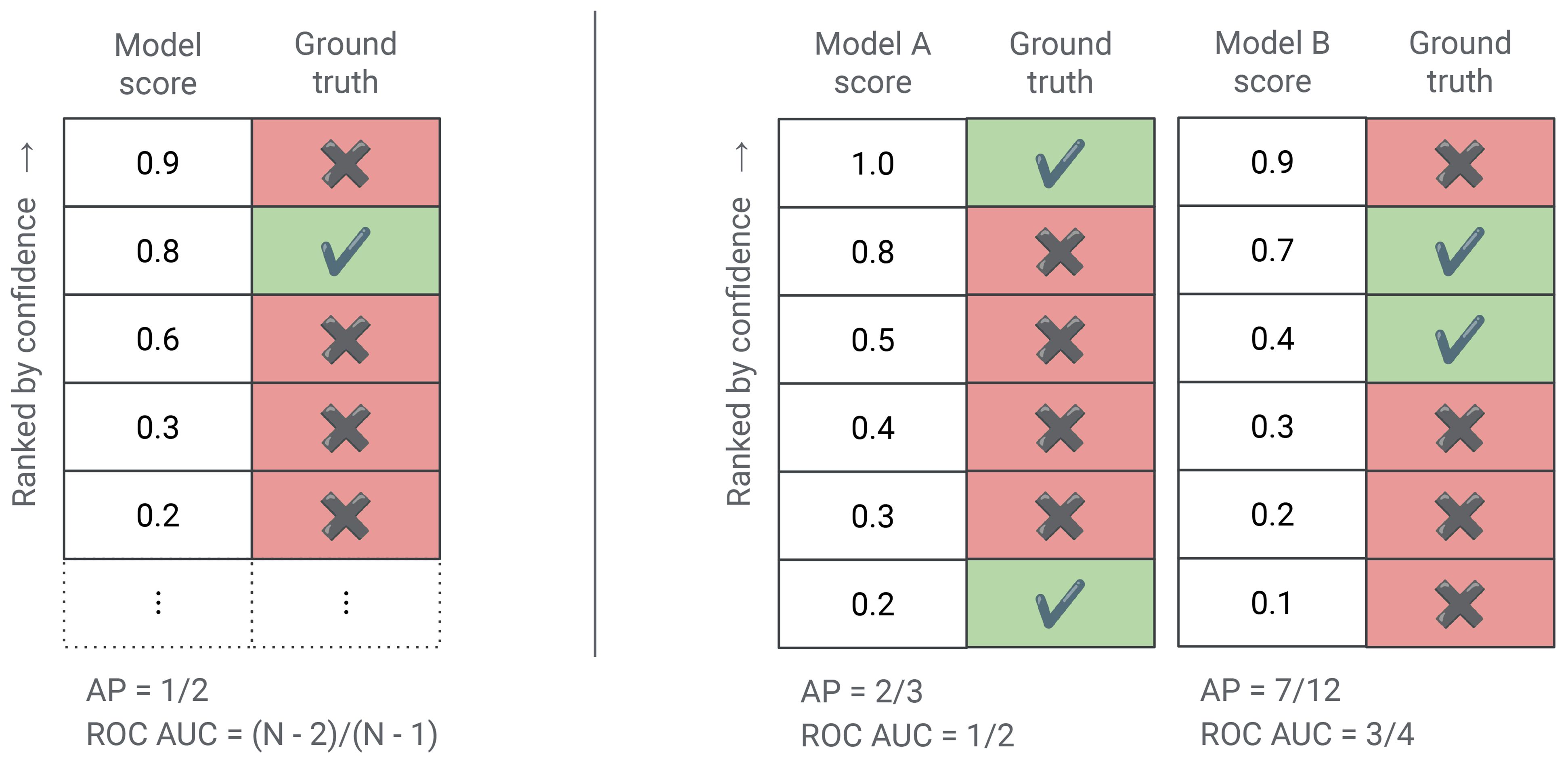
Figure 7 Each row in the figure above is a model prediction (e.g., the presence of a particular bird species in an audio recording) ranked by the model’s confidence score. The first column contains the model’s score and the second column denotes whether the model is in fact correct (e.g., is the bird species actually present according to the ground truth annotation). (Left) This example shows how average precision is only sensitive to the ranking of ground truth positives. There is only a single example in which the bird is actually present. This example is ranked in second place by the model and hence the average precision of this model is 0.5, regardless of the number of ground truth negatives in the dataset. However, if this model was scored using ROC AUC then its score would depend on the number of ground truth negatives. To be precise, the ROC AUC of this model is where N is the total number of examples. (Right) This example compares two models using the same dataset of 6 examples. Which model is better depends on the metric used. Average precision emphasizes early-retrieval performance and prefers the left model, which has an average precision score of compared to for the right model. However, as measured by ROC AUC the right model is better with an ROC AUC score of while the left model has a score of only (no better than random).
ROC AUC has an alternative probabilistic interpretation: When randomly selecting a positive and negative example ranked by the model, it is equal to the probability of the positive example being ranked above the negative (Hanley and McNeil, 1982). This interpretation is very helpful in practice: we can use it to estimate ROC AUC from partial data, and directly reason about model quality. Formally, for a finite dataset D which can be partitioned into positive and negatives examples, the ROC AUC of a model f can be defined as:
where denotes a sample from the partition of positive examples and denotes a sample from the partition of negative examples. This is also equivalent to a scaling of the U statistic from the Mann-Whitney U test (Mason and Graham, 2002).
Another interpretation of ROC AUC relies on considering a ranked list of all predictions: One minus ROC AUC is the average number of negatives ranked above each positive, normalized by the total number of negatives. In this sense, ROC AUC can be thought of as a kind of mean rank metric.
This also shows that ROC AUC a scaling of the information retrieval metric bpref (in the case of complete information; Buckley and Voorhees, 2004). Average precision on the other hand can be thought of as a generalization of mean reciprocal rank.
For event-based evaluation is not possible to calculate the false positive rate which is required to calculate the ROC AUC score, since this requires having ground truth negatives. For this reason, sound event detection often uses the false alarm rate instead (measured as the number of false positives per unit of time; Fiscus et al., 2007). Since this value is no longer bounded by 1, the AUC is calculated by integrating up to a maximum false alarm rate which is considered acceptable for a model. Calculating ROC AUC scores using the false alarm rate can be done in a computationally efficient manner (Ebbers et al., 2022).
3.2 Bias and outlier sensitivity
Metrics such as precision, recall, specificity, and fall-out rate are all biased (Powers, 2020), i.e., the scores of an uninformed classifier will depend on the underlying distribution. This also applies to a derived metric like average precision. Since this means that scores are incomparable across classes with a different number of positive examples, it is inappropriate to average these values across different classes (Figure 8). Alternative (thresholded) unbiased measures to use are informedness, markedness, and the Matthews correlation coefficient (MCC) (Chicco and Jurman, 2020; Chicco et al., 2021). Note that ROC AUC is also an unbiased metric: an uninformed classifier will always have an ROC AUC of 0.5.
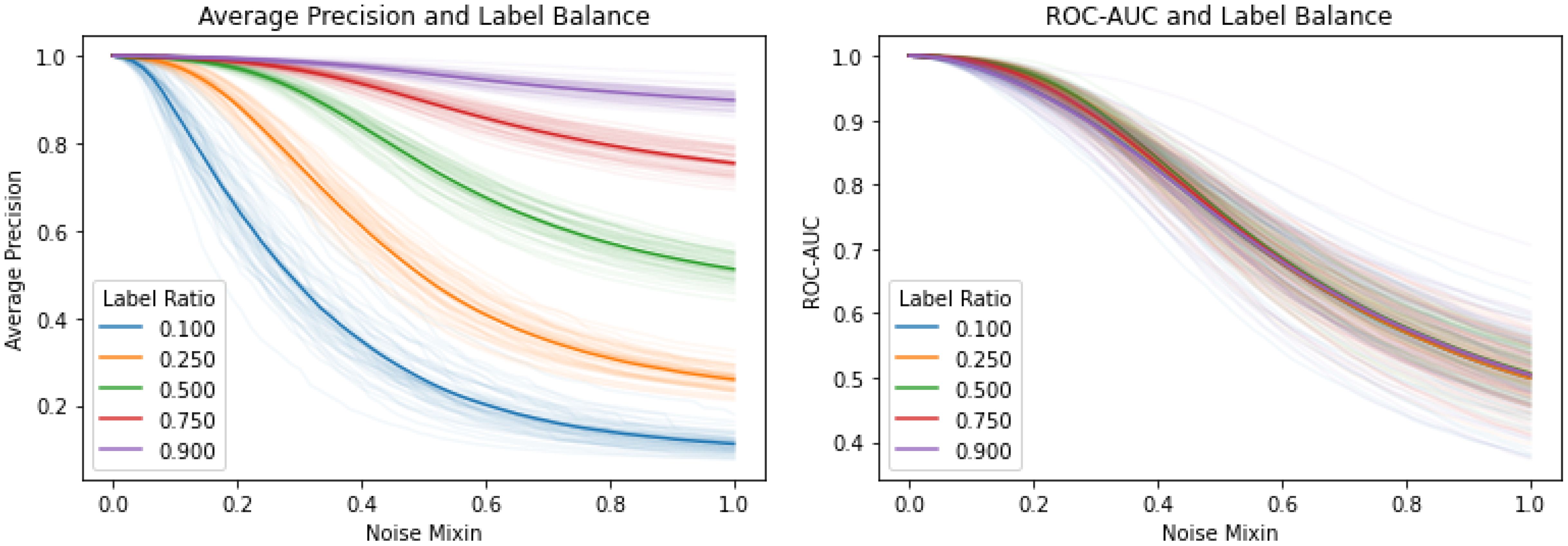
Figure 8 In these figures, the x-axis interpolates linearly between a ‘perfect’ model (with scores evenly spaced between -1.0 and 1.0, and all positive examples given the highest scores) and a noise model (with random unit Gaussian scores). The y-axis gives the interpolated model’s quality according to average precision (left) and ROC AUC (right). We vary the fraction of positives between 10% and 90%, and run with 50 different noise models at each label ratio. Note that average precision is clearly a biased score. As an example of why this is problematic, consider a model which has gotten marginally better at predicting the rare class (e.g., from noise level 0.3 to 0.2) while simultaneously completely forgetting the common class (from noise level 0 to 1). In this case, the mean average precision would increase, while the ROC AUC score would decrease.
That said, even the distribution of unbiased metrics will get skewed as a function of the dataset imbalance (Zhu, 2020), which means that averaging should still be done with care when the data imbalance is widely different across the aggregates.
Another metric property to consider is its sensitivity to outliers. For example, in the case of a single positive example, the average precision score can change from 1.0 to 0.5 if the model ranks the positive example second instead of first. On the other hand, ROC AUC does not have such sensitivity.
3.3 Sample-wise metrics
In segment-based evaluation it is also possible to calculate metrics such as ROC AUC and average precision sample-wise (i.e., rank and score the class labels for each example). When calculating average precision sample-wise this is known as label-ranking average precision (LRAP; Dhivya and Mohandas, 2012). If each sample is then weighted by the number of labels this becomes label-weighted label-ranking average precision (LWLRAP; Howard et al., 2019). It is important to note that these metrics might not be a good reflection of the model’s performance, since a good classifier is not necessarily a good detection model (Table 3).
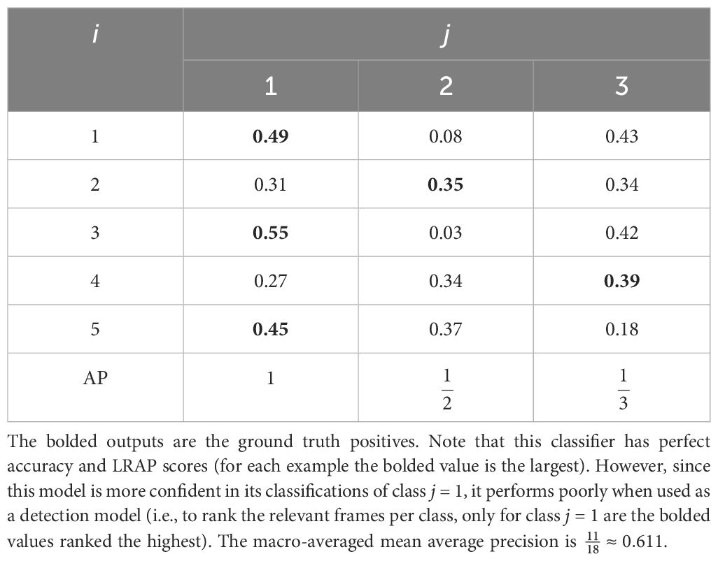
Table 3 A hypothetical set of outputs from a single-label classifier for 5 samples (i, frames) and 3 classes (j) along with the average precision score for each class (AP).
3.4 Multi-class metrics and aggregation
When there are multiple classes, there are a variety of ways in which a final performance score can be calculated. For example, scores (like ROC AUC or average precision) can be calculated separately for each class and then averaged (macro-averaging), or all ground truth annotations can be treated as a single positive class (micro-averaging). Another option is to calculate scores per class and then weight each class by the number of its ground truth annotations (weighted averaging).
Note that in the context of class imbalance, the macro-averaging of unbiased scores like ROC AUC across classes can still result in a score that is no longer insensitive to class imbalance. This is because the ROC AUC score for each class is calculated using a one-vs-rest approach (i.e., any other class is considered a negative) and hence the class imbalance in the “rest” group is no longer taken into account. There exists a multi-class generalization of ROC AUC (Hand and Till, 2001) which avoids this problem by using a one-vs-one approach, calculating and averaging the ROC AUC scores for all possible pairs of classes. Note that this approach is not readily applicable to multi-class sound event detection because there is a single negative (non-event) class which cannot be treated equally to all other classes.
When macro-averaging scores across classes or datasets it is possible to use a variety of means such as the arithmetic, geometric, and harmonic mean. The geometric and harmonic mean reward models for having lower variance in their results (Voorhees, 2003; Robertson, 2006) (i.e., if one model is subject to a larger mean-preserving spread, its final score will be lower). In Bilen et al. (2020) they fit a normal distribution to the class scores and take a low quantile, which has a similar effect. The geometric mean also allows for the calculation of the relative improvement between models (Fuhr, 2018). More complicated methods such as taking the arithmetic mean of the logits of average precision scores have also been proposed (Cormack and Lynam, 2006; Robertson, 2006).
4 Evaluation of out-of-distribution generalization
We argue that robustness to distribution shifts and out-of-distribution generalization are crucial desiderata for foundation models, since their goal is to be general and applicable to a wide array of downstream tasks, each with different characteristics and distributional properties. To this end, we dedicate this section to reviewing literature of related areas that focus on generalization beyond the training distribution, in various forms: domain generalization and adaptation, transfer learning and few-shot learning.
Generally, measuring (and improving upon) the ability of models to generalize from a “source domain” on which they are trained to a different “target domain”, is an important and well-studied issue in machine learning. Different fields focus on studying different instantiations of this generalization problem, by making different assumptions about the relationship between the source and target domains, and the amount and strength of supervision available from the target domain for adaptation.
4.1 Fields studying different facets of generalization
Domain generalization (Zhou et al., 2022) studies the ability of the model to generalize to a target domain “directly” (without using any target data for adaptation). While the target domain has a different distribution from the source, the label set is assumed to be the same. Despite the development of several training algorithms for the specific goal of improving domain generalization performance (Zhou et al., 2022), the literature suggests that training with regular empirical risk minimization and good hyperparameter selection is a strong baseline (Gulrajani and Lopez-Paz, 2020).
Domain adaptation (Wang and Deng, 2018) assumes a similar protocol as domain generalization, with the further assumption of the availability of some unlabeled target examples that can be used for adaptation. Several ideas have been explored, including approaches to encourage domain invariance (Tzeng et al., 2014; Sun and Saenko, 2016; Sankaranarayanan et al., 2018), self-training, by generating pseudolabels for the unlabeled data (Xie et al., 2020), as well as self-supervised learning combined with fine-tuning (Shen et al., 2021).
Transfer learning (Zhuang et al., 2020) is a more general framework that relaxes the assumption that the source and target domains share the same label space or correspond to the same “task” (e.g., one may transfer a model trained for classification to solve a detection task). Consequently, transfer learning protocols typically assume that labeled examples from the target domain are given for adaptation, though the amount of such examples is typically assumed to be less than what is required to train a new model “from scratch” on the target domain.
A common approach to transfer learning in deep learning is to train a linear model on the embeddings produced by one of the intermediate layers of the model (commonly the penultimate layer) (Sharif Razavian et al., 2014). This is sometimes referred to as “linear probing” or using the model as a “fixed feature extractor”. Alternatively, the last layer of the model can be replaced with a new layer after which the entire model is trained (fine-tuned) on the target task (Girshick et al., 2014). Many other advanced methods have been explored in attempts to reduce the computational overhead of fine-tuning (Evci et al., 2022). The ability of a model to transfer to new tasks is often indicative of the overall model quality (Kornblith et al., 2019).
Few-shot learning is a special case of transfer learning where only a few examples are available from the target domain (much fewer than would have been needed to train a target model “from scratch”). While few-shot learning is an instantiation of the more general transfer learning problem, the community has traditionally developed specialized methodology and evaluation practices.
Improving few-shot learning performance has been approached in many ways, involving data augmentation, modelling improvements, or custom training algorithms (Wang et al., 2020b). Some of these techniques require, for example, fine-tuning the source model during evaluation using the few available examples. Other methods do not require any fine-tuning. For example, a simple but strong baseline (Chen et al., 2021) is to build a nearest-centroid classifier in closed form, by estimating one “prototype” (centroid) for each class as the average embedding of the few examples belonging to that class.
Recently, modern large language models have shown impressive few-shot performance during evaluation while not having been explicitly trained for this setting (Brown et al., 2020). This suggests that, under certain circumstances (e.g., in terms of the size of the source dataset, and the relationship between the source and target domains), models may possess the ability to few-shot learn without requiring specialized training recipes.
4.2 Evaluation of generalization
The different fields outlined above have in common the necessity of a “held-out” (set of) dataset(s), domain(s), or task(s) for evaluation, which is a fundamental departure from the standard methodology in machine learning where evaluation takes places on held-out examples of the same dataset, domain, and/or task used for training.
A prominent recent trend in evaluation practices that has been observed across the above fields is the development of more diverse evaluation benchmarks, comprised of several datasets: WILDS for distribution shifts and domain generalization and adaptation (Koh et al., 2021; Sagawa et al., 2021), VTAB for transfer learning (Zhai et al., 2019), and Meta-Dataset (Triantafillou et al., 2019) for few-shot classification, to name a few. This trend has emerged due to the important realization that, to reliably evaluate the ability of a model to transfer from a source to a target domain, we need to account for the variance due to the particular choice of the source and target pair (e.g., by considering several such scenarios). Similarly, we argue that evaluating the generalization properties of bioacoustics foundation models necessitates a wide range of “target domains” and “downstream tasks”. When multiple target datasets or domains are available, either the average or worst-case (Koh et al., 2021) performance across domains is commonly used, with the latter putting a heavier emphasis on robustness3.
Building further on the same argument of variance reduction, few-shot learning in particular requires a specialized evaluation protocol to account for the fact that only a few examples are available in each “target task”, leading to a potential high variance in terms of performance, depending on the specific few examples that were selected. To that end, few-shot learning evaluation adopts an “episodic” evaluation protocol: the model encounters a set of “episodes” at test time, each representing a few-shot learning task, with a different “support set” each time (containing the few available labelled examples), as well as a “query set” (containing held-out examples that the model is asked to predict labels for). The few-shot learning performance that is typically reported is the average performance (e.g., accuracy) on the query set, averaged over a large number of such episodes. We believe that such evaluation practices should serve as inspiration for building evaluation protocols for generalization in bioacoustics too where practitioners are naturally confronted with a plethora of few-shot learning tasks.
While the research community has been very active in studying generalization in the aforementioned fields, most works focus on the vision and language domains. For example, Boudiaf et al. (2023) recently showed that source-free domain adaptation (a challenging variant of domain adaptation) methods developed for vision classifiers perform poorly on a challenging set of distribution shifts in bioacoustics. We thus argue that making progress in building bioacoustics foundation models necessitates the study of different facets of generalization in this domain, which may present different challenges compared to studying generalization in other contexts.
Returning to our running example, few-shot learning for sound event detection (Wang et al., 2020a) can deviate slightly from regular few-shot learning setups. Usually, a few-shot learning problem is defined as having n shots (the number of support examples per class) and k ways (the number of classes). However, in sound event detection only the positives (i.e., the events) are explicitly given. The negatives (non-events) can at most be inferred as being the time periods in between the given events. In a few-shot learning setting this means that the problem must either be approached as a one-way few-shot task (Kruspe, 2019) or by using a method to sample negatives.
Generally, characterizing the commonalities and differences of generalization problems in bioacoustics compared to other domains, and utilizing those findings to build appropriate evaluation frameworks, is an important line of work towards the goal of creating bioacoustics foundation models.
5 Existing efforts in bioacoustics evaluation
There have been a variety of benchmarks and competitions in bioacoustics (Briggs et al., 2013; Karpištšenko et al., 2013; Glotin et al., 2013b). In this section, we will look at the most prominent examples, through the lens of the challenges highlighted throughout this paper (Table 4).
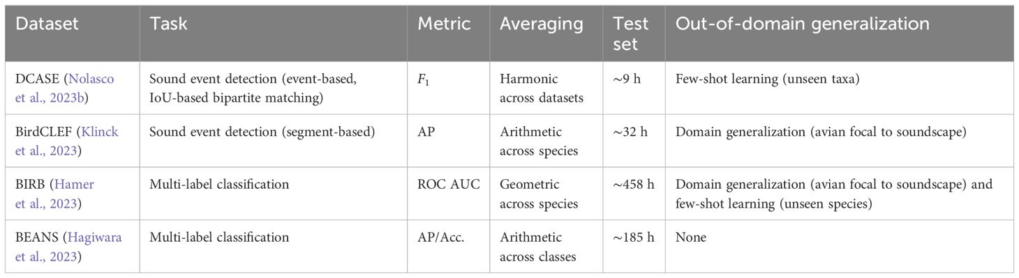
Table 4 An informal comparison of different bioacoustics benchmarks.
An early example, the ICML 2013 Bird Challenge (Glotin et al., 2013a) asked competitors to predict the presence of 35 bird species in a set of recordings which were 150 s long. This challenge already identified domain generalization as an issue (using focal recordings for training but soundscape recordings for testing). The BirdCLEF competition has been running annually since 2014 (Goëau et al., 2014) with gradually increasing dataset sizes. BirdCLEF 2016 (Goëau et al., 2016) was the first edition with an explicit focus on the domain generalization problem from focal to soundscape recordings. The DCASE challenge also introduced a bioacoustic task in 2021 (Morfi et al., 2021) which specifically used a few-shot setting, which has been running annually since. More recently the BIRB bioacoustics information retrieval benchmark (Hamer et al., 2023) and BEANS benchmark of animal sounds (Hagiwara et al., 2023) were introduced, while Ghani et al. (2023) introduced a set of few-shot classification tasks to measure the transfer learning properties of bioacoustics and audio models.
5.1 Sound event detection
Both the DCASE and BirdCLEF challenges evaluate on a sound event detection task. The DCASE challenge uses event-based evaluation whereas the latest BirdCLEF uses segment-based evaluation with a grid of 5 seconds.
The DCASE challenge matches predicted events to ground-truth events by first rejecting all predictions that do not have an IoU of at least 30% with a ground truth event. Then a bipartite matching problem (where the weights are the IoU scores) is solved to find a one-to-one mapping between ground truth and predicted events. The use of IoU in detection is common when matching object detections in vision, since objects in natural images often appear at different scales (closer or further away from the camera), necessitating a scale-invariant metric like IoU. The onset and offset time of an audio event is unlikely to scale with the duration of the event, which is why collars are arguably more appropriate in sound event detection.
DCASE’s usage of a one-to-one mapping between predicted and ground truth events might also not be appropriate for all bioacoustics datasets. For example, for some avian soundscape datasets the annotators were instructed to merge bounding boxes which would be less than 0.5 or 5 seconds apart (Hopping et al., 2022; Navine et al., 2022). Other dataset curators simply instructed annotators that “a series of calls repeated in close succession” would be considered a single annotation (Chronister et al., 2022). Handling such ambiguities would require a framework as proposed by Bilen et al. (2020) (Section 2.2).
Both BIRB and BEANS benchmarks use strongly labeled data for their test set. However, these recordings are segmented into frames which the model must classify separately, reducing the problem to a multi-label classification problem rather than a sound event detection problem. Finally, Ghani et al. (2023) considers classification tasks only.
5.2 Metrics
A variety of metrics have been used by bioacoustics benchmarks and challenges.
The DCASE few-shot bioacoustic event detection task (Nolasco et al., 2023a) uses a thresholded metric, the F1-score. The need for thresholding (e.g., the DCASE baseline system uses a hand-tuned threshold of 0.45) makes it difficult to disentangle the quality of the model from the quality of the threshold. In the case of DCASE the F1-scores are calculated per dataset and then averaged using the harmonic mean to calculate a final score. The harmonic mean puts a strong emphasis on the worst performing dataset.
Note that DCASE ignores events of different classes and considers all events belonging to a single “positive” class. During evaluation this is the same as micro-averaging, which means that the F1-scores represent the class distribution of each dataset. Hence, if the model performs badly on rare classes this is unlikely to show in the scores. Samples-averaging and LWLRAP are metrics with the same property. LWLRAP was used in bioacoustics, for example, in Denton et al. (2022).
The BirdCLEF competitions have generally used macro-averaged average precision under the name class mean average precision (cmAP) (Goëau et al., 2018). Since average precision is a biased metric these scores can be difficult to interpret, as they are heavily dependent on the class imbalance in the test data.
BIRB in contrast opted to use the ROC AUC metric (although in a multi-class setting this is still a biased metric; Section 3.4). Furthermore, it uses geometric averaging of the ROC AUC scores across classes to emphasize worst-case performance (albeit not as strongly as DCASE’s harmonic mean). Use of the geometric mean has seen common usage in fields such as information retrieval (Beitzel et al., 2009).
Both BirdCLEF and BIRB use a macro-averaging strategy where scores are calculated per class and then averaged. This is a good approach when models are to be evaluated for an unknown class distribution at test time. Macro-averaging can be thought of similarly to uninformative priors in Bayesian statistics: in the absence of information about the class distribution at test time, weighting each class equally is reasonable (Figure 9).

Figure 9 An example of a dataset in which one species (yellow, top row) contains more positive ground truth annotations (vocalizations). The precision calculated over all ground truth annotations (micro-averaging) is . If at test time the performance for each species is equally important then this score is not reflective of the model’s performance. A better performance metric could be to take the average of each species’s precision (macro-averaging): .
5.3 Generalization
Measuring the ability of models to generalize out-of-distribution is essential for bioacoustics. The BEANS benchmark is the only benchmark that uses a traditional 6:2:2 split for training, validation, and test data, and as such does not measure out-of-distribution generalization.
Most other bioacoustics benchmarks do directly measure out-of-distribution generalization in some way. The BirdCLEF competitions have long used a domain generalization framework where focal recordings from Xeno-Canto are used as training data while evaluating on soundscape recordings (Kahl et al., 2022a).
DCASE explicitly uses a few-shot setup with separate datasets for training and testing. While birds appear in both the training and test, several other species are unique to the test set. As such, the benchmark measures not only the ability of the model to learn from few examples, but also the model’s ability to generalize to new datasets and species.
Ghani et al. (2023) evaluate a variety of birdsong models in a few-shot learning setting on a new set of datasets. They train a linear classifier on the frozen embeddings. Like DCASE they evaluate the performance on held-out datasets containing vocalizations from unseen species and tasks, such as bird call types, marine mammals, frogs, and bats.
BIRB, like BirdCLEF, uses focal recordings from Xeno-Canto as training data while using soundscapes for testing, evaluating the model partly in a domain generalization setup. However, it additionally leaves out species from specific geographies (e.g., Hawai’i and Colombia) from the training data, allowing it to explicitly evaluate generalization to new species in a few-shot learning task.
6 Conclusion
Progress towards bioacoustics foundation models requires the careful design of evaluation procedures that reflect the practical utility of the models. As we have discussed in depth, this is challenging for several reasons. Notably, the bioacoustics data that is available has limitations in terms of coverage (e.g., geographic coverage, species abundance) and we do not have sufficient large-scale training data reflecting all possible deployment conditions (types of annotations, microphones), which unavoidably leads to distribution shifts between training and evaluation data. Further, as discussed, certain distributional characteristics of bioacoustics data (e.g., their long-tailed nature) pose challenges with regards to evaluation metrics too: we do not necessarily want to reward a model that does well on average but consistently fails to make correct predictions on data points in the “tail”. We argue, therefore, for the necessity of “general-purpose” robust bioaoustics models that are able to cope well with a variety of distribution shifts and generalize to deployment conditions and novel species rapidly. Crucially, carefully crafting good evaluation practices is a key ingredient in incentivizing and supporting the development of bioacoustics models with the desired characteristics.
As a first step towards that goal, we have reviewed existing evaluation practices in bioacoustics, aiming to identify drawbacks and opportunities for improvement. Specifically, we reviewed the way that sound event detection tasks are evaluated in the literature, which metrics can be used to quantify model quality, and how model robustness and adaptability can be explicitly measured in the frameworks of domain generalization, transfer learning, and few-shot learning. Finally, we have discussed the multitude of design decisions made by existing bioacoustics benchmarks and challenges. Ultimately, there is no single way in which a model’s ability to generalize and adapt can be measured, since this depends on the type of tasks and data distributions the model will be deployed on. Hence, designing benchmarks that reflect a model’s real-world utility requires careful consideration of how the data, model and evaluation protocol interact. We hope that the topics raised in this review will help assist in the development of such benchmarks, and by extension, the development of stronger bioacoustics models.
Author contributions
BM: Conceptualization, Visualization, Writing – original draft, Writing – review & editing. JH: Writing – review & editing. VD: Visualization, Writing – review & editing. ET: Writing – review & editing. TD: Writing – review & editing.
Funding
The author(s) declare that no financial support was received for the research, authorship, and/or publication of this article.
Conflict of interest
All authors are employed by Google.
Publisher’s note
All claims expressed in this article are solely those of the authors and do not necessarily represent those of their affiliated organizations, or those of the publisher, the editors and the reviewers. Any product that may be evaluated in this article, or claim that may be made by its manufacturer, is not guaranteed or endorsed by the publisher.
Footnotes
- ^ The evaluation of a model’s ability to correctly predict the frequency of a vocalization is left out of the scope of this review.
- ^ Note that the metric proposed in Bilen et al. (2020) seemingly has strange behaviour in extreme cases: A model could get perfect recall and a false alarm rate of by making a single prediction which spans the full recording. This could be addressed by using a false alarm rate which calculates the duration (rather than number) of false positives per recording.
- ^ The geometric and harmonic mean would be other options that lie in between these two choices.
References
Beitzel S. M., Jensen E. C., Frieder O. (2009). GMAP (Boston, MA: Springer US), 1256–1256. doi: 10.1007/978–0-387–39940-9493
Bilen C., Ferroni G., Tuveri F., Azcarreta J., Krstulović S. (2020). “A framework for the robust evaluation of sound event detection,” in Proceedings of the International Conference on Acoustics, Speech and Signal Processing. (IEEE), 61–65.
Bjorck J., Rappazzo B. H., Chen D., Bernstein R., Wrege P. H., Gomes C. P. (2019). Automatic detection and compression for passive acoustic monitoring of the african forest elephant. Proc. AAAI Conf. Artif. Intell. 33, 476–484. doi: 10.1609/aaai.v33i01.3301476
Bommasani R., Hudson D. A., Adeli E., Altman R., Arora S., von Arx S., et al. (2021). On the opportunities and risks of foundation models. arXiv preprint arXiv:2108.07258. doi: 10.48550/arXiv.2108.07258
Borsos Z., Marinier R., Vincent D., Kharitonov E., Pietquin O., Sharifi M., et al. (2023). Audiolm: a language modeling approach to audio generation. IEEE/ACM Trans. Audio Speech Lang. Process. 31, 2523–2533. doi: 10.1109/TASLP.2023.3288409
Boudiaf M., Denton T., van Merriënboer B., Dumoulin V., Triantafillou E. (2023). In search for a generalizable method for source free domain adaptation. arXiv preprint arXiv:2302.06658. doi: 10.48550/arXiv.2302.06658
Briggs F., Huang Y., Raich R., Eftaxias K., Lei Z., Cukierski W., et al. (2013). “The 9th annual mlsp competition: New methods for acoustic classification of multiple simultaneous bird species in a noisy environment,” in 2013 IEEE International Workshop on Machine Learning for Signal Processing (MLSP). (IEEE), 1–8. doi: 10.1109/MLSP.2013.6661934
Brown T., Mann B., Ryder N., Subbiah M., Kaplan J. D., Dhariwal P., et al. (2020). Language models are few-shot learners. Adv. Neural Inf. Process. Syst. 33, 1877–1901. doi: 10.48550/arXiv.2005.14165
Buckley C., Voorhees E. M. (2004). “Retrieval evaluation with incomplete information,” in Proceedings of the 27th Annual International ACM SIGIR Conference on Research and Development in Information Retrieval (Association for Computing Machinery), SIGIR ‘04. (ACM), 25–32. doi: 10.1145/1008992.1009000
Callaghan C. T., Nakagawa S., Cornwell W. K. (2021). Global abundance estimates for 9,700 bird species. Proc. Natl. Acad. Sci. 118, e2023170118. doi: 10.1073/pnas.2023170118
Cao C., Chicco D., Hoffman M. M. (2020). The mcc-f1 curve: a performance evaluation technique for binary classification. arXiv preprint arXiv:2006.11278. doi: 10.48550/arXiv.2006.11278
Chen Y., Liu Z., Xu H., Darrell T., Wang X. (2021). “Meta-baseline: Exploring simple meta-learning for few-shot learning,” in Proceedings of the IEEE/CVF international conference on computer vision. (IEEE/CVF), 9062–9071.
Chicco D., Jurman G. (2020). The advantages of the matthews correlation coefficient (mcc) over f1 score and accuracy in binary classification evaluation. BMC Genomics 21, 1–13. doi: 10.1186/s12864-019-6413-7
Chicco D., Tötsch N., Jurman G. (2021). The matthews correlation coefficient (mcc) is more reliable than balanced accuracy, bookmaker informedness, and markedness in two-class confusion matrix evaluation. BioData Min. 14, 1–22. doi: 10.1186/s13040-021-00244-z
Chronister L. M., Rhinehart T. A., Place A., Kitzes J. (2022). An annotated set of audio recordings of Eastern North American birds containing frequency, time, and species information. Zenodo. doi: 10.5061/dryad.d2547d81z
Clapp M., Kahl S., Meyer E., McKenna M., Klinck H., Patricelli G. (2023). A collection of fully-annotated soundscape recordings from the southern Sierra Nevada mountain range. Zenodo. doi: 10.5281/zenodo.7525805
Conde M. V., Shubham K., Agnihotri P., Movva N. D., Bessenyei S. (2021). Weakly-supervised classification and detection of bird sounds in the wild. a birdclef 2021 solution. arXiv preprint arXiv:2107.04878. doi: 10.48550/arXiv.2107.04878
Cormack G. V., Lynam T. R. (2006). “Statistical precision of information retrieval evaluation,” in Proceedings of the 29th annual international ACM SIGIR conference on Research and development in information retrieval. (ACM), 533–540.
Denton T., Wisdom S., Hershey J. R. (2022). “Improving bird classification with unsupervised sound separation,” in ICASSP 2022–2022 IEEE International Conference on Acoustics, Speech and Signal Processing (ICASSP). (IEEE), 636–640.
Dhivya S., Mohandas P. (2012). “Comparison of convolutional neural networks and k-nearest neighbors for music instrument recognition,” in Advances in Speech and Music Technology: Computational Aspects and Applications. (Springer), 175–192.
Diblíková L., Pipek P., Petrusek A., Svoboda J., Bílková J., Vermouzek Z., et al. (2019). Detailed large-scale mapping of geographical variation of yellowhammer emberiza citrinella song dialects in a citizen science project. Ibis 161, 401–414. doi: 10.1111/ibi.12621
Ebbers J., Haeb-Umbach R., Serizel R. (2022). “Threshold independent evaluation of sound event detection scores,” in ICASSP 2022–2022 IEEE International Conference on Acoustics, Speech and Signal Processing (ICASSP). (IEEE), 1021–1025.
Evci U., Dumoulin V., Larochelle H., Mozer M. C. (2022). “Head2toe: Utilizing intermediate representations for better transfer learning,” in International Conference on Machine Learning. (PMLR), 6009–6033.
Fiscus J. G., Ajot J., Garofolo J. S., Doddingtion G. (2007). Results of the 2006 spoken term detection evaluation. Proc. sigir 7, 51–57.
Franco M., Lipani C., Bonaventure O., Nijssen S. (2020). automated monitoring of bat species in Belgium. Louvain-la-Neuve, Belgium: Anglais, Ph. D. dissertation, UCL-Ecole polytechnique de Louvain.
Fuhr N. (2018). “Some common mistakes in ir evaluation, and how they can be avoided,” in Acm sigir forum, vol. 51. (New York, NY, USA: ACM), 32–41.
Ghani B., Denton T., Kahl S., Klinck H. (2023). Global birdsong embeddings enable superior transfer learning for bioacoustic classification. Nature 13. doi: 10.1038/s41598-023-49989-z
Gibb R., Browning E., Glover-Kapfer P., Jones K. E. (2019). Emerging opportunities and challenges for passive acoustics in ecological assessment and monitoring. Methods Ecol. Evol. 10, 169–185. doi: 10.1111/2041-210X.13101
Girshick R., Donahue J., Darrell T., Malik J. (2014). “Rich feature hierarchies for accurate object detection and semantic segmentation,” in Proceedings of the IEEE conference on computer vision and pattern recognition. (IEEE), 580–587.
Glotin H., Clark C., LeCun Y., Dugan P., Halkias X., Jérôme S. (2013a). The 1st International Workshop on Machine Learning for Bioacoustics (Atlanta, GA: ICML).
Glotin H., LeCun Y., Artières T., Mallat S., Tchernichovski O., Halkias X. (2013b). Neural Information Processing Scaled for Bioacoustics: From Neurons to Big Data (Stateline, NV: NeurIPS).
Goëau H., Glotin H., Vellinga W.-P., Planqué R., Joly A. (2016). “Lifeclef bird identification task 2016: The arrival of deep learning,” in CLEF: Conference and Labs of the Evaluation Forum, Vol. 1609. 440–449.
Goëau H., Glotin H., Vellinga W.-P., Planqué R., Rauber A., Joly A. (2014). “Lifeclef bird identification task 2014,” in CLEF: Conference and Labs of the Evaluation forum, Vol. 1180. 585–597.
Goëau H., Kahl S., Glotin H., Planqué R., Vellinga W.-P., Joly A. (2018). “Overview of birdclef 2018: monospecies vs. soundscape bird identification,” in CLEF 2018-Conference and Labs of the Evaluation Forum, Vol. 2125.
Gulrajani I., Lopez-Paz D. (2020). In search of lost domain generalization. arXiv preprint arXiv:2007.01434. doi: 10.48550/arXiv.2007.01434
Hagiwara M., Hoffman B., Liu J.-Y., Cusimano M., Effenberger F., Zacarian K. (2023). “Beans: The benchmark of animal sounds,” in ICASSP 2023–2023 IEEE International Conference on Acoustics, Speech and Signal Processing (ICASSP). (IEEE), 1–5.
Hamer J., Triantafillou E., van Merrienboer B., Kahl S., Klinck H., Denton T., et al. (2023). BIRB: A generalization benchmark for information retrieval in bioacoustics. arXiv preprint arXiv:2312.07439. doi: 10.48550/arXiv.2312.07439
Hand D. J., Till R. J. (2001). A simple generalisation of the area under the roc curve for multiple class classification problems. Mach. Learn. 45, 171–186. doi: 10.1023/A:1010920819831
Hanley J. A., McNeil B. J. (1982). The meaning and use of the area under a receiver operating characteristic (roc) curve. Radiology 143, 29–36. doi: 10.1148/radiology.143.1.7063747
Hopping W. A., Kahl S., Klinck H. (2022). A collection of fully-annotated soundscape recordings from the Southwestern Amazon Basin. Zenodo. doi: 10.5281/zenodo.7079124
Hutchinson B., Rostamzadeh N., Greer C., Heller K., Prabhakaran V. (2022). “Evaluation gaps in machine learning practice,” in Proceedings of the 2022 ACM Conference on Fairness, Accountability, and Transparency (Association for Computing Machinery), FAccT ‘22. (ACM), 1859–1876. doi: 10.1145/3531146.3533233
Kahl S., Denton T., Klinck H., Glotin H., Goëau H., Vellinga W.-P., et al. (2021a). “Overview of birdclef 2021: Bird call identification in soundscape recordings,” in CLEF (Working Notes). 1437–1450.
Kahl S., Navine A., Denton T., Klinck H., Hart P., Glotin H., et al. (2022a). “Overview of birdclef 2022: Endangered bird species recognition in soundscape recordings,” in Working Notes of CLEF.
Kahl S., Wood C. M., Chaon P., Peery M. Z., Klinck H. (2022b). A collection of fully-annotated soundscape recordings from the Western United States. Zenodo. doi: 10.5281/zenodo.7050014
Kahl S., Wood C. M., Eibl M., Klinck H. (2021b). Birdnet: A deep learning solution for avian diversity monitoring. Ecol. Inf. 61, 101236. doi: 10.1016/j.ecoinf.2021.101236
Karpištšenko A., Spaulding E., Cukierski W. (2013). The marinexplore and cornell university whale detection challenge.
Kiskin I., Sinka M., Cobb A. D., Rafique W., Wang L., Zilli D., et al. (2021). Humbugdb: a large-scale acoustic mosquito dataset. arXiv preprint arXiv:2110.07607. doi: 10.48550/arXiv.2110.07607
Koh P. W., Sagawa S., Marklund H., Xie S. M., Zhang M., Balsubramani A., et al. (2021). “Wilds: A benchmark of in-the-wild distribution shifts,” in International Conference on Machine Learning. (PMLR), 5637–5664.
Kornblith S., Shlens J., Le Q. V. (2019). “Do better imagenet models transfer better?,” in Proceedings of the IEEE/CVF conference on computer vision and pattern recognition. (IEEE/CVF), 2661–2671.
Kruspe A. (2019). One-way prototypical networks. arXiv preprint arXiv:1906.00820. doi: 10.48550/arXiv.1906.00820
Laiolo P. (2010). The emerging significance of bioacoustics in animal species conservation. Biol. Conserv. 143, 1635–1645. doi: 10.1016/j.biocon.2010.03.025
Martin A. F., Doddington G. R., Kamm T., Ordowski M., Przybocki M. A. (1997). The det curve in assessment of detection task performance. Eurospeech 4, 1895–1898. doi: 10.21437/Eurospeech.1997
Mason S. J., Graham N. E. (2002). Areas beneath the relative operating characteristics (roc) and relative operating levels (rol) curves: Statistical significance and interpretation. Q. J. R. Meteorological Soc. 128, 2145–2166. doi: 10.1256/003590002320603584
Mcloughlin M. P., Stewart R., McElligott A. G. (2019). Automated bioacoustics: Methods in ecology and conservation and their potential for animal welfare monitoring. J. R. Soc. Interface 16, 20190225. doi: 10.1098/rsif.2019.0225
Mesaros A., Heittola T., Virtanen T. (2016). Metrics for polyphonic sound event detection. Appl. Sci. 6, 162. doi: 10.3390/app6060162
Mesaros A., Heittola T., Virtanen T., Plumbley M. D. (2021). Sound event detection: A tutorial. IEEE Signal Process. Magazine 38, 67–83. doi: 10.1109/MSP.2021.3090678
Moreno-Torres J. G., Raeder T., Alaiz-Rodríguez R., Chawla N. V., Herrera F. (2012). A unifying view on dataset shift in classification. Pattern recognition 45, 521–530. doi: 10.1016/j.patcog.2011.06.019
Morfi V., Nolasco I., Lostanlen V., Singh S., Strandburg-Peshkin A., Gill L. F., et al. (2021). “Few-shot bioacoustic event detection: A new task at the dcase 2021 challenge,” in DCASE, 145–149.
Navine A., Kahl S., Tanimoto-Johnson A., Klinck H., Hart P. (2022). A collection of fully-annotated soundscape recordings from the Island of Hawai’i. Zenodo. doi: 10.5281/zenodo.7078499
Nolasco I., Ghani B., Singh S., Vidaña Vila E., Whitehead H., Grout E., et al. (2023a). Few-shot bioacoustic event detection at the dcase 2023 challenge. Ecol. Inform. 77.
Nolasco I., Singh S., Morfi V., Lostanlen V., Strandburg-Peshkin A., Vidaña-Vila E., et al. (2023b). Learning to detect an animal sound from five examples. Ecol. Inf. 77, 102258. doi: 10.1016/j.ecoinf.2023.102258
Penar W., Magiera A., Klocek C. (2020). Applications of bioacoustics in animal ecology. Ecol. complexity 43, 100847. doi: 10.1016/j.ecocom.2020.100847
Powers D. M. (2020). Evaluation: from precision, recall and f-measure to roc, informedness, markedness and correlation. arXiv preprint arXiv:2010.16061. doi: 10.48550/arXiv.2010.16061
Pratap V., Xu Q., Sriram A., Synnaeve G., Collobert R. (2020). Mls: A large-scale multilingual dataset for speech research. arXiv preprint arXiv:2012.03411. doi: 10.48550/arXiv.2012.03411
Quinonero-Candela J., Sugiyama M., Schwaighofer A., Lawrence N. D. (2008). Dataset shift in machine learning (Boston, MA: Mit Press). doi: 10.7551/mitpress/9780262170055.001.0001
Radford A., Kim J. W., Hallacy C., Ramesh A., Goh G., Agarwal S., et al. (2021). “Learning transferable visual models from natural language supervision,” in International conference on machine learning. (PMLR), 8748–8763.
Ranft R. (2004). Natural sound archives: past, present and future. Anais da Academia Bras. Cienciasˆ 76, 456–460. doi: 10.1590/S0001-37652004000200041
Robertson S. (2006). “On gmap: and other transformations,” in Proceedings of the 15th ACM international conference on Information and knowledge management. (ACM), 78–83.
Saeed A., Grangier D., Zeghidour N. (2021). “Contrastive learning of general-purpose audio representations,” in ICASSP 2021–2021 IEEE International Conference on Acoustics, Speech and Signal Processing (ICASSP). (IEEE), 3875–3879.
Sagawa S., Koh P. W., Lee T., Gao I., Xie S. M., Shen K., et al. (2021). Extending the wilds benchmark for unsupervised adaptation. arXiv preprint arXiv:2112.05090. doi: 10.48550/arXiv.2112.0509
Saito T., Rehmsmeier M. (2015). The precision-recall plot is more informative than the roc plot when evaluating binary classifiers on imbalanced datasets. PloS One 10, e0118432. doi: 10.1371/journal.pone.0118432
Sankaranarayanan S., Balaji Y., Castillo C. D., Chellappa R. (2018). “Generate to adapt: Aligning domains using generative adversarial networks,” in Proceedings of the IEEE conference on computer vision and pattern recognition. (IEEE/CVF), 8503–8512.
Sayigh L., Daher M. A., Allen J., Gordon H., Joyce K., Stuhlmann C., et al. (2016). The watkins marine mammal sound database: an online, freely accessible resource. Proc. Meetings Acoustics 4ENAL (Acoustical Soc. America) 27, 040013. doi: 10.1121/2.0000358
Schütze H., Manning C. D., Raghavan P. (2008). Introduction to information retrieval Vol. 39 (Cambridge, UK: Cambridge University Press Cambridge).
Sharif Razavian A., Azizpour H., Sullivan J., Carlsson S. (2014). “Cnn features off-the-shelf: an astounding baseline for recognition,” in Proceedings of the IEEE conference on computer vision and pattern recognition workshops. (IEEE/CVF), 806–813.
Shen K., Jones R. M., Kumar A., Xie S. M., Liang P. (2021). How does contrastive pre-training connect disparate domains?
Sofaer H. R., Hoeting J. A., Jarnevich C. S. (2019). The area under the precision-recall curve as a performance metric for rare binary events. Methods Ecol. Evol. 10, 565–577. doi: 10.1111/2041-210X.13140
Stewart R., Andriluka M., Ng A. Y. (2016). “End-to-end people detection in crowded scenes,” in Proceedings of the IEEE conference on computer vision and pattern recognition. (IEEE/CVF), 2325–2333.
Stowell D. (2022). Computational bioacoustics with deep learning: a review and roadmap. PeerJ 10, e13152. doi: 10.7717/peerj.13152
Sugai L. S. M., Silva T. S. F., Ribeiro J., Wagner J., Llusia D. (2018). Terrestrial passive acoustic monitoring: review and perspectives. BioScience 69, 15–25. doi: 10.1093/biosci/biy147
Sun B., Saenko K. (2016). “Deep coral: Correlation alignment for deep domain adaptation,” in Computer Vision–ECCV 2016 Workshops: Amsterdam, The Netherlands, October 8–10 and 15–16, 2016, Proceedings, Part III 14. (Netherlands: Springer Amsterdam), 443–450.
Swamidass S. J., Azencott C.-A., Daily K., Baldi P. (2010). A croc stronger than roc: measuring, visualizing and optimizing early retrieval. Bioinformatics 26, 1348–1356. doi: 10.1093/bioinformatics/btq140
Teixeira D., Maron M., van Rensburg B. J. (2019). Bioacoustic monitoring of animal vocal behavior for conservation. Conserv. Sci. Pract. 1. doi: 10.1111/csp2.72
Triantafillou E., Zhu T., Dumoulin V., Lamblin P., Evci U., Xu K., et al. (2019). Meta-dataset: A dataset of datasets for learning to learn from few examples. arXiv preprint arXiv:1903.03096. doi: 10.48550/arXiv.1903.03096
Tzeng E., Hoffman J., Zhang N., Saenko K., Darrell T. (2014). Deep domain confusion: Maximizing for domain invariance. arXiv preprint arXiv:1412.3474. doi: 10.48550/arXiv.1412.3474
Vega-Hidalgo A., Kahl S., Symes L. B., Ruiz-Gutiérrez V., Molina-Mora I., Cediel F., et al. (2023). A collection of fully-annotated soundscape recordings from neotropical coffee farms in Colombia and Costa Rica. Zenodo. doi: 10.5281/zenodo.7525349
Vellinga W.-P., Planqué R. (2015). “The Xeno-Canto collection and its relation to sound recognition and classification,” in Conference and Labs of the Evaluation Forum.
Voorhees E. M. (2003). “Overview of the trec 2003 robust retrieval track,” in Trec. (NIST: Gaithersburg, MD), 69–77.
Wang M., Deng W. (2018). Deep visual domain adaptation: A survey. Neurocomputing 312, 135–153. doi: 10.1016/j.neucom.2018.05.083
Wang Y., Salamon J., Bryan N. J., Bello J. P. (2020a). “Few-shot sound event detection,” in ICASSP 2020–2020 IEEE International Conference on Acoustics, Speech and Signal Processing (ICASSP). (IEEE), 81–85. doi: 10.1109/ICASSP40776.2020
Wang Y., Yao Q., Kwok J. T., Ni L. M. (2020b). Generalizing from a few examples: A survey on few-shot learning. ACM computing surveys (csur) 53, 1–34. doi: 10.1145/3386252
Xie Q., Luong M.-T., Hovy E., Le Q. V. (2020). “Self-training with noisy student improves imagenet classification,” in Proceedings of the IEEE/CVF conference on computer vision and pattern recognition. (IEEE/CVF), 10687–10698.
Zhai X., Kolesnikov A., Houlsby N., Beyer L. (2022). “Scaling vision transformers,” in Proceedings of the IEEE/CVF Conference on Computer Vision and Pattern Recognition (CVPR). (IEEE/CVF), 12104–12113.
Zhai X., Puigcerver J., Kolesnikov A., Ruyssen P., Riquelme C., Lucic M., et al. (2019). A large-scale study of representation learning with the visual task adaptation benchmark. arXiv preprint arXiv:1910.04867. doi: 10.48550/arXiv.1910.04867
Zhou K., Liu Z., Qiao Y., Xiang T., Loy C. C. (2022). Domain generalization: A survey. IEEE Trans. Pattern Anal. Mach. Intell. 45, 4396–4415. doi: 10.1109/TPAMI.2022.3195549
Zhu Q. (2020). On the performance of matthews correlation coefficient (mcc) for imbalanced dataset. Pattern Recognition Lett. 136, 71–80. doi: 10.1016/j.patrec.2020.03.030
Keywords: bioacoustics, passive acoustic monitoring, sound event detection, metrics, transfer learning, few-shot learning, foundation models
Citation: van Merriënboer B, Hamer J, Dumoulin V, Triantafillou E and Denton T (2024) Birds, bats and beyond: evaluating generalization in bioacoustics models. Front. Bird Sci. 3:1369756. doi: 10.3389/fbirs.2024.1369756
Received: 12 January 2024; Accepted: 10 June 2024;
Published: 01 July 2024.
Edited by:
Cristian Pérez-Granados, University of Alicante, SpainReviewed by:
Irene Mendoza, Spanish National Research Council (CSIC), SpainThiago Ventura, Federal University of Mato Grosso, Brazil
Copyright © 2024 van Merriënboer, Hamer, Dumoulin, Triantafillou and Denton. This is an open-access article distributed under the terms of the Creative Commons Attribution License (CC BY). The use, distribution or reproduction in other forums is permitted, provided the original author(s) and the copyright owner(s) are credited and that the original publication in this journal is cited, in accordance with accepted academic practice. No use, distribution or reproduction is permitted which does not comply with these terms.
*Correspondence: Bart van Merriënboer, YmFydHZtQGdvb2dsZS5jb20=