Diversity is key: fantasy football dream teams under budget constraints

Given a fixed budget for player salaries, what is the distribution of salaries of the top scoring teams? We investigated this question using the wealth of data available from fantasy premier league football (soccer). Using the players’ data from past seasons, for several seasons and several different budget constraints, we identified the highest scoring fantasy team for each season subject to each budget constraint. We then investigated quantifiable characteristics of these teams. Interestingly, across nearly every variable that is significant to the game of football and the budget, these top teams display diversity across these variables. Furthermore, randomly assembled teams would statistically not display such diversity across these variables. Our results indicate that diversity across these variables, including salaries, is a general feature of top performing teams. Moreover, in the process of obtaining these results we developed a data cleaning (or data reduction) algorithm that drastically reduced the amount of data to be analyzed.

1 Introduction

Sports have fascinated and entertained people for thousands of years (Thuillier, 2004). People enjoy not only playing sports but also being a fan and cheering for their favorite competitor or team. Fans also like to place wagers on sporting events and competitions (Holt, 2011). Sports betting has a long history dating back thousands of years, like in ancient Rome where bets could be placed at chariot races (Lanciani, 2024). Betting on sports continued through the years into modern times, and today sports betting is a major industry attracting billions of customers (Saul, 2022).

While one can bet on real-life matches, fantasy sports allow fans to play the role of team manager and bet on the fantasy teams they create. Fantasy sports are a class of multiplayer games based on real life sport players’ performances. They date back to at least the 1950s when Wilfred Winkenbach created fantasy golf (Kissell and Poserina, 2017; Ruihley and Chamberlin, 2021). Fantasy sports were introduced to academia in 1960 when Harvard University sociologist William Gamson started the “Baseball Seminar” where colleagues would form rosters that earned points based on the players’ final standings in batting average, RBI, ERA, and wins (Davis and Duncan, 2006; Gamson, 1975). The landmark “Rotisserie League” was also based on Major League Baseball and founded by Daniel Okrent in the 1980s (Ploeg, 2021). Fantasy sports gained tremendous popularity during the 1990s as widespread internet access became available (Ruihley and Chamberlin, 2021), with the foundation of the Fantasy Sports Trade Association in 1998 (Billings and Ruihley, 2013). Over 50 million Americans play fantasy sports (Foster et al., 2020; King and LeBoulluec, 2017; Dyreson, 2019). In India, there are around 100 million users playing Fantasy cricket (Brettenny et al., 2012; Adhikari et al., 2020; Naha, 2021; Karthik et al., 2021; Kaur and Jagdev, 2020). Globally, fantasy sports is a multibillion dollar industry (South et al., 2019; Ruihley et al., 2021).

Anyone can play fantasy football for free. In Fantasy Premier League (FPL), you begin with a budget of 100 million pounds and act as the manager of a Premier League football team. Adhering to your budget, you select fifteen players: two goalkeepers, five defenders, five midfielders, and three forwards. The basic aim of FPL is to accumulate as many points as possible across the season. From your squad of 15 players, you must select a starting XI (eleven) for each game week. A game week usually consists of 10 games played during the season. The players you select for each game week receive points based on their real-world performances. You can put your team in any formation, although there must always be one goalkeeper, at least three defenders and at least one forward selected at all times. There are many further details involved in playing FPL which can be found on the official FPL homepage.

Unlike playing FPL, however, real-life team managers have different budgets for their teams. It is therefore natural to ask, what is the best team one can create for a specific budget? Using the available FPL data from past seasons, we investigate how many points all possible starting XI, subject to different budget constraints, score. In this way, for each budget, we identify the best possible team one could create. We reasonably expect the insights gained by the compositions of these teams may be useful and interesting in both real-world and fantasy sports. Moreover, the methods we use to obtain our results may be of further interest, because a priori there is an impossibly large number of calculations required to analyze all possible teams that could be created within a given season. For example, in season 2016–2017, there were 684 active players. Considering all possible starting XI that could be formed with these players amounts to $\left(\genfrac{}{}{0ex}{}{684}{11}\right)\approx 10^{23}$combinations. Calculating the scores of all of these teams could not be achieved in a human lifetime.

In spite of this seemingly insurmountable number of combinations, for 11 budget constraints, we determined for each budget constraint the best team according to total points earned by its players during a season. We did this for five seasons starting from the 2016–2017 season and continuing to the 2020–2021 season. We defined the lowest budget in order to compare teams comprised of players that actually had game time, because the absolute cheapest players often did not have any game time. The highest budget was based on the best team one could build without imposing any budget constraint. Starting from the lowest budget and increasing incrementally to the highest budget resulted in a total of 11 budget constraints. We then investigated the compositions and characteristics of the best teams for all 11 budgets for all five seasons. Although we characterized the best teams cumulatively over an entire season, the same approach could be used iteratively to provide insights for trades to make during a season. Moreover, our data reduction methods that allowed us to analyze a seemingly impossibly large data set could be of independent interest due to its theoretical basis and therewith lack of constraint to any single field of application.

1.1 Outline

This work is organized as follows. In §2, we describe our methods. Our results are presented in §3, and a discussion of both our methods and results concludes this study in §4.

2 Methods: data collection, reduction, and analysis

We used data collected from five Fantasy Premier League (FPL) seasons, starting with the 2016–2017 (2017) season and continuing through the 2020–2021 (2021) season. We gathered the Premier League season data from the FPL websites’ API with permission from FPL. Since only the current season is available on the websites’ API, we obtained data for the previous seasons from a GitHub repository (Vaastav, 2013) which has collected data from several FPL seasons. We used the data to calculate all players’ summary statistics over a full season. The variables we used to construct the best teams were the cost at the end of the season and the total points gathered for the whole season. We also needed the position of each player, denoted element_type. For notational convenience, we use the numbers 1, 2, 3, 4 to represent each of the four positions: goalkeeper, defender, midfielder, forward, respectively. In the 2017 season there were 684 players, and in 2021 there were 714 players. Each player was assigned a unique identifying number, known as the player id. So, in 2017 this number is between 1 and 684. We organized the player id, cost, total points, and element type as shown in Table 1. This is only a tiny fraction of the data. In order to handle the large amount of data, we developed a data reduction algorithm which we describe in the following subsection.

Table 1

Table 1. This is an example of four rows of data from a fantasy season.

2.1 Data reduction

If we were to calculate all fantasy teams that could theoretically be created during a single season, this would require a few thousand years with our best algorithm on a standard computer. In the seasons analyzed, the total number of players is on the order of 700, and the number of all possible combinations of 11 players is on the order $\left(\genfrac{}{}{0ex}{}{700}{11}\right)\approx 10^{23}$. Of course, not all such theoretical teams are possible, because a team must have one of the allowed formations (goalkeeper-defenders-midfielders-forwards): 1-3-4-3, 1-3-5-2, 1-4-4-2, 1-4-5-1, 1-4-3-3, 1-5-3-2 and 1-5-4-1. Imposing this restriction does not reduce the amount of calculations to a manageable quantity. Instead, we realized that to determine the highest scoring team subject to a specific budget constraint, it is not necessary to consider all fantasy teams. With this in mind, we created a data reduction algorithm that significantly reduced the number of teams in each budget bracket. This type of algorithm could be used for other analyses that compare a certain metric of performance subject to one or more constraints on resources.

The data reduction algorithm discards players that we can rigorously prove would never be among the best eleven for a specific budget constraint. For example, in Table 1, as long as there are midfielders who earned at least one point and whose cost are at most 43, then those players dominate player # 31, since they have the same or lower cost but strictly higher points. In general, a player with a higher cost and lower number of points would never be chosen as part of the best eleven if there are cheaper player(s) of the same type (position) with higher points. Consequently, one of the main functions in our data reduction algorithm is to remove players of the same element type (position) that are strictly dominated in the sense that there are cheaper players with higher points. The full algorithm removes the data in a series of steps. The first three steps compare individual players of the same element type (position). The fourth step compares collections of players of the same element type in the case of defenders, midfielders, and forwards, because formations can have different numbers of these positions as explained in Table 2. The fifth and final step compares these position groups starting from the lowest cost, and iteratively increasing the cost. If increasing the cost does not yield higher points, then those more expensive groups are dominated by the cheaper groups and can therefore be safely removed. In the end, the algorithm reduced the number of combinations to analyze to determine the best team subject to all budget constraints from the order of $10^{23}$ to the order of $10^7$. We now explain this precise steps of our algorithm.

Table 2

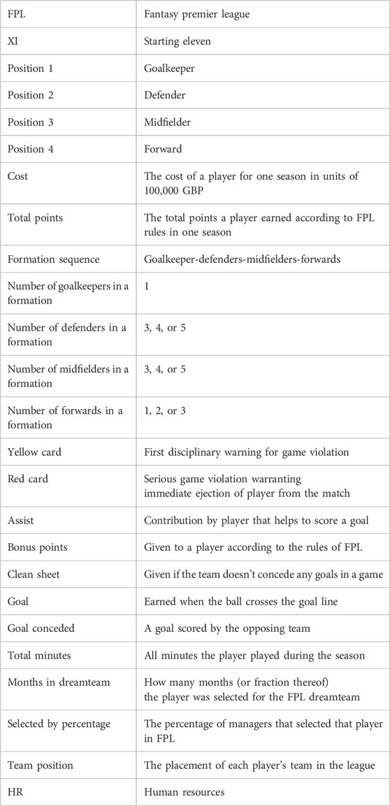
Table 2. Here we collect the variables and notation in this study.

2.1.1 The five steps of the data reduction process

In the first three steps of the data reduction process, only players of the same element type (position) are compared. We first compare players with the same cost and keep only those with the most points. Those with the same cost and lower points are deleted. An example of this is shown in Table 3. Next, we compare players with the same number of points and keep only those with the lowest costs. Those with the same points and higher costs are deleted. An example of this is shown in Table 4. In the third step, we compare players with cost $C$ to those with cost $C+1$. If a player has cost $C+1$ and less points than the players we have kept at this point with cost $C$ then they are deleted. The rest are kept. An example of the third step is shown in Table 5. These three steps are summarized in Figure 1.

Table 3

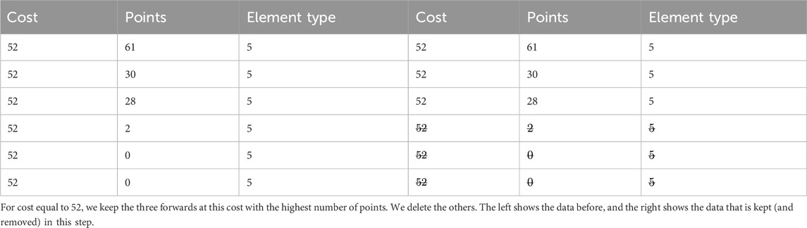
Table 3. This shows an example of the first step in our data reduction algorithm.

Table 4

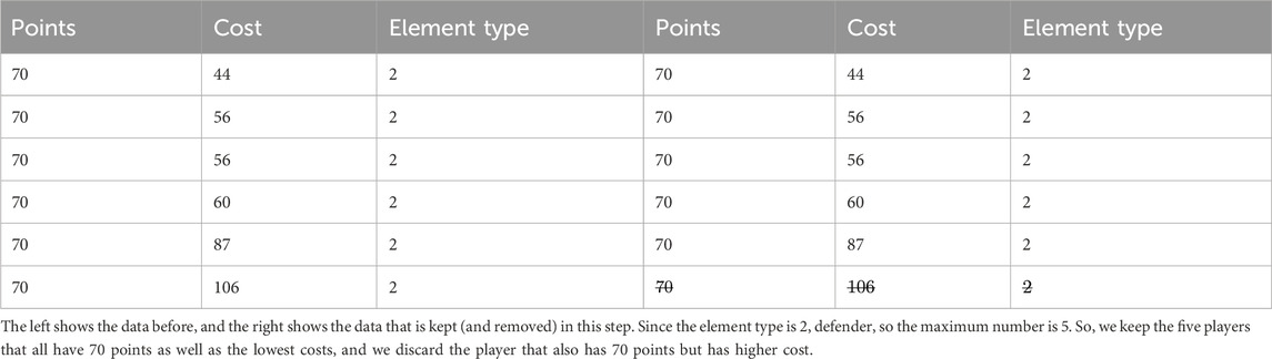
Table 4. This shows an example of the second step in our data reduction algorithm.

Table 5

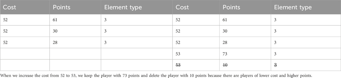
Table 5. This shows the third step in our data reduction process.

Figure 1

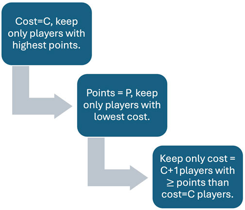
Figure 1. In the first three steps of the data reduction process we compare the individual players of each element type. In the first step we compare all players with the same cost and keep only those with highest points. Next we compare all players with the same points and keep only those with the lowest cost. Finally we compare the cost $=C+1$ players to the cost $=C$ players and keep only those $C+1$ cost players with points greater than or equal to the cost $=C$ players. We repeat this for each element (position) type. All data that is not kept is deleted.

The fourth step in our data reduction process compares collections of players in each element type. Essentially, we repeat the first three steps for each element type, except goalies, because there is one goalie in any formation. The fourth step is shown in the case of defenders in Figure 2.

Figure 2

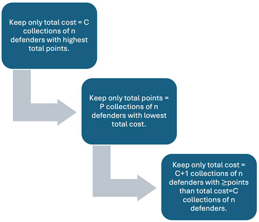
Figure 2. In the fourth step of the data reduction process we compare collections of players of each element type. For defenders we do this for $n=\mathrm{3,4,5}$ since there could be $\mathrm{3,4}$ or five defenders. We then do the same for midfielders. For forwards, we do this for $n=\mathrm{1,2,3}$. For each value of $n$, we compare all collections of $n$ players with the same total cost and keep only those with highest points. Next we compare all collections of $n$ players with the same points and keep only those with the lowest cost. Finally we compare the cost$=C+1$ collections to the cost$=C$ collections and keep only those cost$=C+1$ with points greater than or equal to the cost$=C$. We repeat this for each element (position) type: defender, midfield, forward.

Algorithm 1

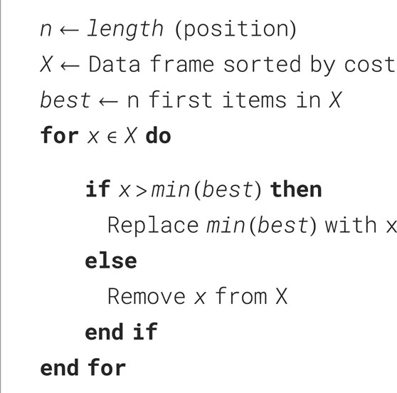
Algorithm 1. When increasing the total cost we are able to pick more players with a higher cost, but this is only advantageous if those players also have higher points than the players with lower costs. This algorithm checks whether the team gets more total points if we select the new players that we can afford when increasing the budget. If we don’t use the new players because they will not increase the total points, then we discard them.

In the fifth and last step of the data reduction process, we sorted these position groups in ascending order of cost, starting with the lowest cost. So, for example, since the number of goalkeepers is always one, at each cost there is precisely one goalkeeper, namely the goalkeeper with the highest points for that cost. For defenders, we could have either 3, 4, or 5 defenders for a given cost. Starting with the lowest cost, we save the points that the first combination had as a reference. If we increased the cost and did not receive higher points than the reference points, we discarded that combination. If we received higher total points, we set our reference as this new total point value and continued looping through all combinations. This is Algorithm 1.

Finally, having reduced the data, we analyzed all possible position sets from the remaining data according to the allowed formations (goalkeeper-defenders-midfielders-forwards): 1-3-4-3, 1-3-5-2, 1-4-4-2, 1-4-5-1, 1-4-3-3, 1-5-3-2 and 1-5-4-1. With these considerations, once we had assembled all the possible teams for all possible formations, we had approximately $7\times 10^7$ total teams to analyze. These algorithms therewith decreased the number of teams from on the order of $10^{23}$ to the order of $10^7$. Our data is available on github, as well as the data reduction algorithms in Python.

2.2 Integer programming approach to calculating the highest scoring team within each budget constraint

After reducing the data, one could work with the reduced data set to calculate the highest scoring team within each budget constraint by formulating an integer programming (IP) problem. To do this we represent our data set as vectors in ${\mathbb{R}}^7$. The first four components indicate the type of player. A player of type $j$ has one in the $j^{th}$ component and 0 in the three other of the first four components. The fifth component of the vector is the cost of the player. The sixth component of the vector is their total points, and the seventh component is their ID. Then, one selects 11 vectors from our (reduced) data set and computes their sum, denoted $s$. The problem is then to maximize $s\cdot e_6$ subject to the constraints corresponding to the allowed formations and the budget: $s\cdot e_1=1,3\le s\cdot e_2\le 5,3\le s\cdot e_3\le 5,1\le s\cdot e_4\le 3$, $s\cdot e_5\le \text{budget\hspace{0.17em}constraint.}$ This problem can be solved in python with the following code as shown in Algorithm 2. The results of running this code, which we call lp-problem. py, are contained in our github repository, and the results of this code agree with the results of our original algorithm. We further note that this is a variation of the classic knapsack problem which consists of choosing an optimal subset of a set to carry in a knapsack of fixed size. In this problem, optimal means the subset that fits within the knapsack and has the maximum value.

Algorithm 2

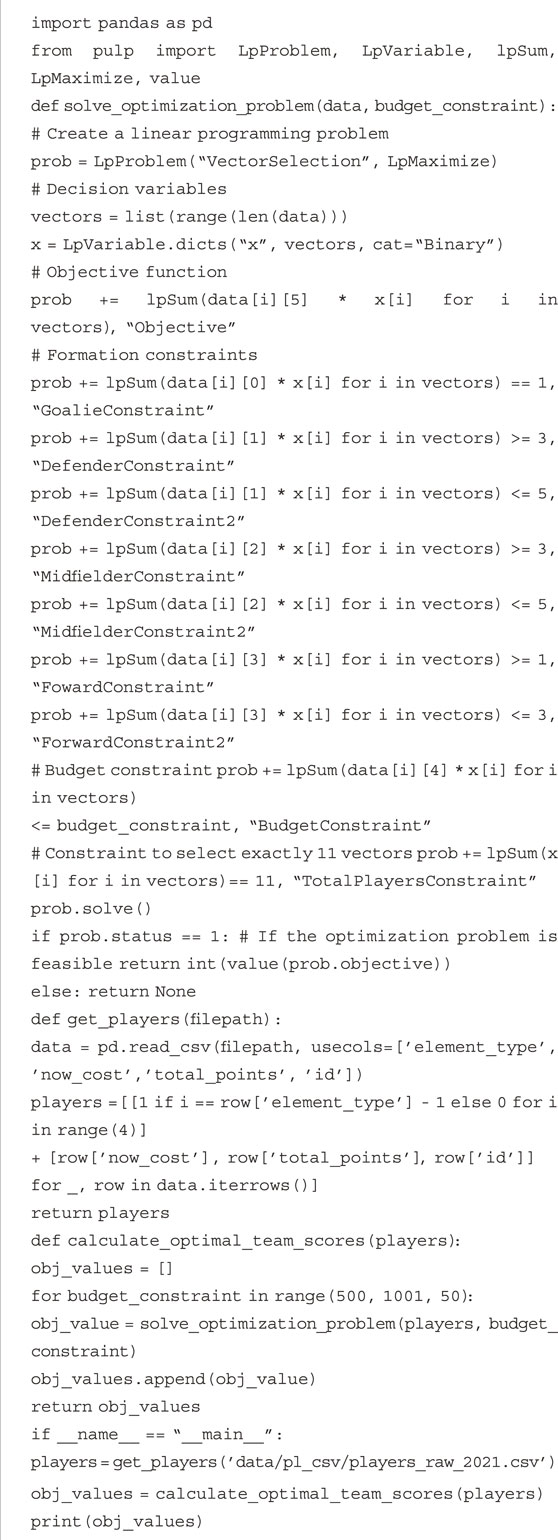
Algorithm 2. Integer programming formulation in python for finding the best team within each budget constraint.

2.3 Analyzing the salary distributions

In the previous subsections, we showed how to reduce the data to a manageable quantity and then calculate the highest scoring teams subject to a given budget constraint. Once we determined these ‘dream teams,’ we then analyzed different variables that are essential to football as shown in Table 2. Perhaps the most important variable is money. A team manager has a budget: a limited amount of money that they can spend on the team. How should they spend this budget on the players? What are the salary distributions of the best performing teams? Is the distribution similar to a normal distribution, with several players earning close to the average salary and a few outliers? Or are there a few star players with very high salaries and several players with much lower salaries? Or is there a wide range of salaries, dispersed somewhat evenly across the interval ranging from the lowest to the highest? If this is the case, we would describe the distribution as diverse. We could ask the same question regarding the distribution of other variables that are essential to performance, like assists and goals. How are the values of these variables across the players? Are the values clumped like a normal distribution, or are they more evenly spread out across a range, like a diverse distribution?

Algorithm 3

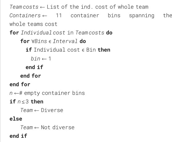
Algorithm 3. Algorithm to determine if a team is diverse based on the bin approach.

In Rowlett et al. (2022) developed a game theoretic model that analyzes competition between teams of individuals subject to a resource constraint. There they show that a diverse distribution of resources across the team’s individuals is associated with team success in competition. With this motivation, we introduced an intuitive ‘bin-method’ to classify distributions as diverse or not. For each team we calculated an eleven step interval grid. At each step we made a subinterval, or bin, such that the union of all sub-intervals is the full range of the variable under consideration. For each team, we looped through all the individual players’ values of the particular variable under consideration, and then we sorted them into the appropriate bins. If there were no empty bins, then we consider the distribution of that particular variable to be diverse, because it is analogous to the diverse distribution in the discrete model from Rowlett et al. (2022). However, since reality is not perfect or necessarily perfectly aligned with mathematical theorems like those of Rowlett et al. (2022), here we still classify a distribution as diverse if a few of the bins are empty. Thus, a distribution with at most $three$ empty bins is considered a diverse distribution. The code for this classification is shown in Algorithm 3.

3 Results: the dream teams

We investigated the teams that performed the best within each budget constraint, and here present the analysis made on two seasons, 2017 and 2019, due to space limitations. The budgets, total cost, and total points are shown in Table 6. However, interested readers are referred to Gullholm and Stålberg (2022) for further details of other seasons and further analyses. It may also be interesting to note the total cost and total points for the best teams within each budget constraint in six for the 2021 season.

Table 6

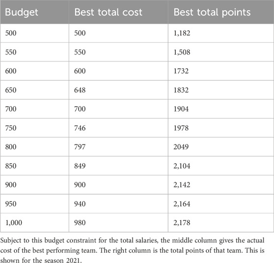
Table 6. The maximum budget is in the left column given in units 100,000 GBP.

When we analysed the total points for the best teams under each budget we obtained that the points increased logarithmically. As one would expect, the team with the highest points possible is that with the highest budget. The name, cost, and points of all the players in the best team with the highest budget for the 2021 season is show in Table 7.

Table 7

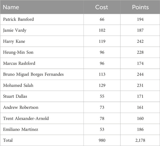
Table 7. This is the name, cost and points of all the players in the best team under budget 1,000 for season 2021.

3.1 Formations

We also analysed which formation that gave the best result for each budget. The results can be seen in Figure 3. We can see that three formations stood out, namely 3-5-2, 4-5-1 and 5-4-1. When taking the mean of the best position for each budget we can see an interesting trend, visualised in Figure 3: for a lower budget it is preferable to have more defenders and fewer forwards, while for a higher budget it is the opposite.

Figure 3

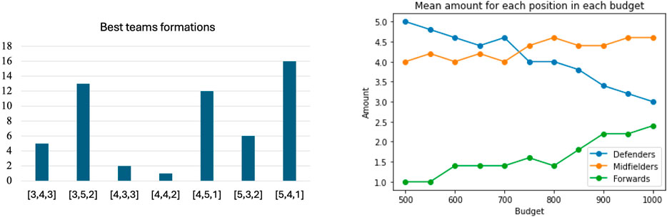
Figure 3. The left figure compares the frequency of the possible formations within the highest scoring teams in each budget class. There, count refers to the number of times the formation shown on the horizontal axis was the highest scoring within its budget class. The right figure shows the mean cost of each position subject to each budget constraint. The budget is shown on the horizontal axis. Amount on the vertical axis refers to the number of players of each of the three types in the best team with the budget given on the horizontal axis.

3.2 Salary distributions within the best teams

We investigated the salary distributions of the best teams in every formation and budget. The total number of best teams is

$5\ast 7\ast 11=385$

because we assessed 5 seasons, 7 formations, and 11 budgets in FPL. Figure 4 shows that 72% of the best teams’ salary distributions were considered diverse. The distributions of costs between the players were similar when we checked all seasons separately and when we combined the players from all seasons. Motivated by this fact, we analyzed teams that could contain players from different seasons. In this analysis, 69% of the best teams were considered to be diverse. Consequently, we observe that a diverse salary distribution is a predominant characteristic of the best preforming FPL teams.

Figure 4

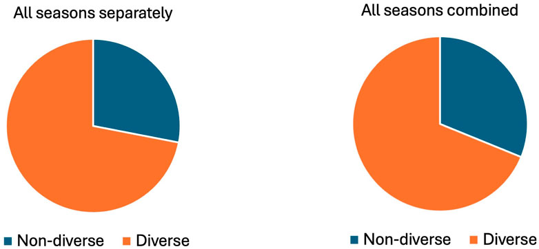
Figure 4. This figure shows the percentage of best teams in all budgets that have diverse or non diverse salary distributions. On the left, we calculated the best teams for each season separately, for each budget constraint. Of these, 277 are diverse while 108 are not diverse, thus 72% have diverse salary distributions. On the right, we calculated the best teams for each budget constraint, allowing players to be selected from any of the five seasons. Of these, 53 are diverse while 24 are not diverse, thus 69% have diverse salary distributions.

We note that if a team were chosen completely randomly, then the probability that the salary distribution would be classified as diverse is quite low, because the majority of players have nearly identical salaries; see Figure 5. Approximately 33% of the players have salaries in a single bin, so with a purely randomly chosen team, approximately 33% of the team, or 4 players, would have salaries contained in a single bin. Moreover, there are two additional salary bins of players with approximately 120 players per bin. So, similarly, with a purely randomly chosen team, at least approximately 2 more players would also have salaries contained in a single bin. Consequently, a purely randomly chosen team is unlikely to have a diverse salary distribution, because 6 players would have salaries contained within just 2 bins. Consequently, even if all the other 5 players’ salaries were contained in different bins, there would still be 4 empty bins, resulting in a non-diverse salary distribution.

Figure 5

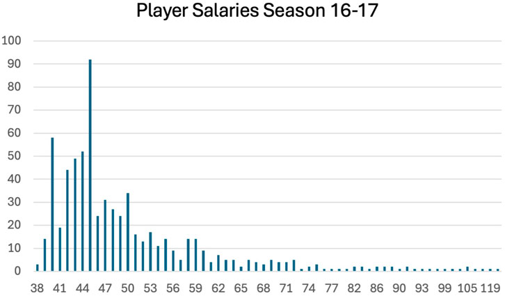
Figure 5. This shows the distribution of salaries across all players for the 2016–2017 season. There are approximately 700 players in each of the seasons. Approximately 230 players have the same salaries, corresponding to about 33% of all the players.

3.3 Distributions of other variables within the best teams

A diverse salary distribution is a characteristic that is common to the majority of the most successful FPL teams as shown in §3.2; see Figure 4. As one can see from Figure 5, a randomly chosen team is unlikely to have a diverse salary distribution. Is there diversity in other variables within the best teams? We assessed this for several variables that are essential to football. The results for the different variables are presented in Figure 6. Each colored dot represents the mean value for each sorted (according to cost) player. The black dots represent the mean for each budget. The variables we assessed are essential to football:

• Yellow cards.

• Assists.

• Bonus points: given to a player according to the rules of FPL.

• Clean sheets: if the team doesn’t concede any goal.

• Mean costs for different budgets for seasons 2017 to 2021.

• Goals.

• Goals conceded.

• Total minutes: all minutes the player played during the season.

• Months in Dreamteam: how many months the player was selected to the Dreamteam.

• Selected by percentage: how many percentage of managers that selected that player.

• Team position: the placement of each players team in the league.

• Red cards.

The distributions for 11 of these 12 variables are diverse. The only variable with a non-diverse distribution is the number of red cards. This may indicate that it is better to have more players that all contribute different amounts across a range of values, rather than having just a few star players carrying the team. With the exception of red cards, there is a large spread within each variable and budget constraint, corresponding to diversity across these variables.

Figure 6

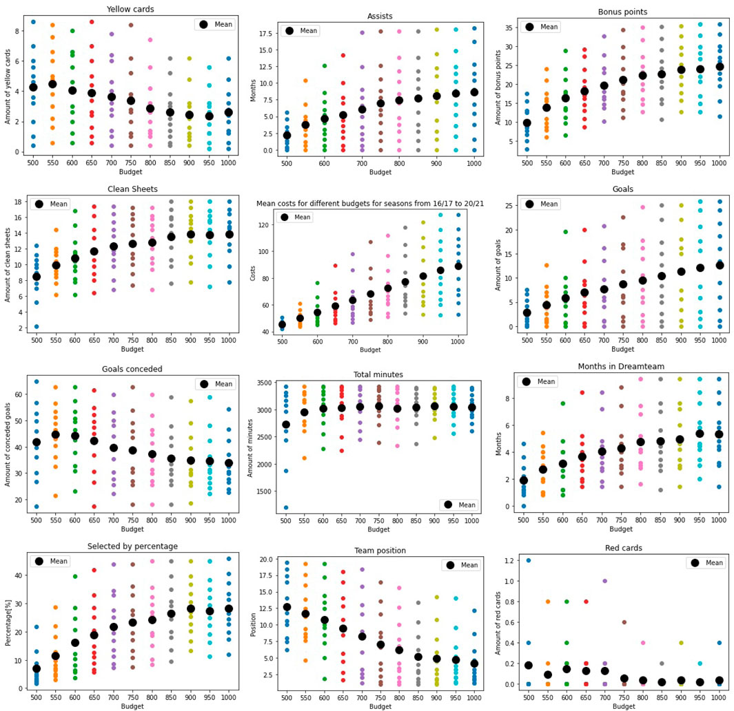
Figure 6. The distribution of different variables for the best teams in the FPL seasons. The black dots represent the mean of each variable for each budget. The colored dots show the values for each player sorted according to cost.

4 Discussion

Can one predict the fantasy team which would score the highest points in an upcoming football season? Or, could one identify fantasy teams which are likely to be among the highest scoring in the next season? Although we cannot answer these questions with the present study, we have made a fundamental step towards prediction by analyzing the characteristics of top performing teams with a range of budgets for the players’ salaries. Our results here show that diversity is a common feature of these top performing teams.

4.1 The role of diversity and the diversity theorems

There may be a more general underlying mechanism through which diversity amongst team members is beneficial to the team in competition with other teams. Indeed, this concept within high performing teams dates back to at least the 1980s; see, for example, the Belbin model (Belbin, 1981). There, Belbin considered different types of contributors in a team and showed that teams with these different types of contributors generally perform well. Belbin’s work is based on psychology and empirical studies. More recently, Rowlett et al. has formulated a purely theoretical mathematical approach for analyzing competing teams in Rowlett et al. (2022). The Diversity Theorems in Rowlett et al. (2022), show that a team performs better if the individuals within it are diverse with regard to any competitive ability with a budget constraint on this competitive ability. The Diversity Theorems are based on a game-theoretic model for competing teams comprised of individuals. The individuals of a team each have a competitive ability that determines their success or defeat in competition with an individual from an opposing team. Identical competitive abilities result in a tie, whereas different competitive abilities result in a win for the individual with the higher ability and a loss for the individual with the lower ability. The team’s success is calculated by amassing all cumulative wins and losses of the team’s individuals. If no constraint is imposed on the competitive ability values, then to achieve the strongest possible team, one would simply let the competitive ability values tend to infinity. However, if a constraint is imposed, then certain distributions of competitive abilities amongst individuals outperform others. The Diversity Theorems identify the best way to distribute competitive abilities subject to a constraint on the mean competitive ability. There, a specific way of distributing competitive abilities is called a strategy. The Diversity Theorems show that the best strategies are those that assign individuals a diverse range of competitive abilities (Rowlett et al., 2022). It is interesting to note that although the scientific approaches of Belbin (1981) and Rowlett et al. (2022) are completely different, the results sound quite similar.

4.2 Competitive ability in theory and practice

One of major the challenges of utilizing the Diversity Theorems is to interpret the real-world meaning of ‘competitive ability.’ This is one of the motivations for our investigation here of professional sports, because there is a correlation between an individual player’s salary and their performance (Yaldo and Shamir, 2017). Identifying a player’s salary with their competitive ability allows us to investigate the theoretical predictions. Moreover, the ‘mean competitive ability’ (mca) constraint of Rowlett et al. (2022) is equivalent to having a budget constraint for the salaries of the team. This is a natural and realistic constraint, because every real-life team has a limited budget from which to pay the players’ salaries. We note, however that ‘competitive ability’ is a mathematical concept, so it could be used to describe any trait. Consequently, we analyzed not only the salary distributions but also the distributions across several other variables that are essential to football as shown in Figure 6. With both the salary distribution as well as the distributions across all variables (except red cards) demonstrated in Figures 4, 6, respectively, the diversity observed across all these different variables shows that, in general, diversity is a prevalent characteristic of the best performing teams. This echoes the theoretical predictions of the Diversity Theorems (Rowlett et al., 2022) and the Belbin’s empirical studies (Belbin, 1981).

In Peddii and Jain (2023), the authors developed a machine-learning model using a random forest algorithm that they claim is “capable of predicting the performance of individual players and generating a predicted optimal team lineup.” Their assessment is based on a notion of ‘in form’ or ‘out of form.’ This could be compared to our notion of competitive ability, but with binary values, rather than assuming values over a range. Another approach was proposed in Toda et al. (2022). As they observe “conventional evaluation methods based on predictions of scores are considered unreliable because they predict rare events throughout the game.” Instead, they suggest that ball recovery and being attacked may be more effective in predicting game success. In de Jong et al. (2020), the authors analyzed several variables and concluded that the variables in women’s soccer that are most useful for predicting success are: scoring first, intentional assists relative to the opponent, the percentage of shots on goal saved by the goalkeeper relative to the opponent, shots on goal relative to the opponent, and the percentage of duels that are successful. In Phatak et al. (2022), the authors analyze several KPIs in football, using FPL data similar to our study. Their aim was to identify methods for effective use of machine learning and artificial intelligence to predict team success in the specific context of both fantasy and real-life football. In the meta-analysis (Bunker and Susnjak, 2022) they reviewed studies from 1996 to 2019 that used machine learning for predicting match results. They observed that although artificial neural networks were commonly applied in early studies, their findings suggest that a range of models should be compared. This also fits with the theoretical predictions of the diversity theorems. It would be interesting to investigate combining our approach with other methods like these and analyze to what extent we can predict successful FPL team compositions.

4.3 Data reduction algorithms

One of the contributions of this work is our data reduction algorithm. Numerous algorithms have been developed to reduce superfluous, corrupt, duplicate, or otherwise irrelevant data (Wang et al., 2017; Barat et al., 2014). Most algorithms seem to be focused on removing data that is damaged or duplicate, rather than removing data according to an optimization process as in our algorithm. Our context is somewhat similar to feature selection processes (FS) (Alweshah et al., 2022). However, the closest context to ours seems to be the study of knapsack problems and algorithms developed to efficiently solve these problems in the context of large data sets (Ali et al., 2021). There has been quite a lot of research dedicated to efficient solutions; see Jooken et al. (2023) for an overview as well as references therein. Our data reduction algorithm may also be compared to data summarization processes that select representative subsets of manageable size out of massive data, as well as submodular optimization problems. According to Han et al. (2021), “although there exist extensive algorithms for submodular optimization, many of them incur large computational overheads and hence are not suitable for mining big data.” Consequently, our algorithm could be complementary to existing algorithms, because it runs simply and efficiently.

4.4 Statistical limitations

Our study uses aggregated data from five seasons of premier league football. It may be susceptible to misinterpretation due to Simpson’s paradox. There is also the possibility for error due to manual data collection techniques.

4.5 Outlook

Motivated by the results of this paper, further research should focus on generalizing the performed analyses to other contexts: Is diversity key only for fantasy football? What about other teams? Both the Belbin model (Belbin, 1981) and the Diversity Theorems (Rowlett et al., 2022) indicate the relevance of diversity. In this paper we managed to transfer these theoretical truths to practice. However, this is only the first step. While our analyses can be applied to almost all teams where we have a constraint (such as the budget) and a measurable performance (such as scores), the results need to be checked for other contexts. For example, software projects require a diverse knowledge distributed among the team members. A couple of years ago, the idea of so-called cross-functional teams that have almost all required knowledge in the team, emerged in research and practice (Beck et al., 2001). Having all required knowledge in the team is also an aspect of diversity. Having only members with a similar set of skills and knowledge would be less beneficial. However, so far, there is no approach showing how to form a team given a number of possible team members. Transferring the results presented in this paper to such a context would not only influence the work of HR (human resource) managers by helping to determine which skills the new team member needs in order to increase the team’s diversity, but also affect the collaboration and the knowledge sharing in the teams.

In this direction, it would also be interesting to analyze how diversity changes over time. That is, if one starts with a diverse team, how do the characteristics of players or team members influence the performance of others within the team? Does diversity decrease over time as, for example, knowledge or techniques are shared with the other team members? In the context of hypothetical teams (as we have in fantasy football) this line of thought cannot be analyzed, because these team members are not actually on the same team. Therefore, transferring this idea to real teams would be interesting. We propose that further research should focus on strengthening the results obtained here and analyzing them with regard to the applicability in other contexts such as HR.

Data availability statement

Publicly available datasets were analyzed in this study. This data can be found here: https://github.com/vaastav/Fantasy-Premier-League/tree/master/data}{GitHub repository}.

Author contributions

JG: Conceptualization, Data curation, Formal Analysis, Investigation, Methodology, Project administration, Resources, Software, Validation, Visualization, Writing–original draft, Writing–review and editing. JK: Conceptualization, Data curation, Formal Analysis, Funding acquisition, Investigation, Methodology, Project administration, Resources, Software, Supervision, Validation, Writing–original draft, Writing–review and editing. JR: Conceptualization, Formal Analysis, Funding acquisition, Investigation, Methodology, Project administration, Resources, Software, Supervision, Validation, Writing–original draft, Writing–review and editing. JS: Conceptualization, Data curation, Formal Analysis, Investigation, Methodology, Project administration, Resources, Software, Validation, Visualization, Writing–original draft, Writing–review and editing.

Funding

The author(s) declare that no financial support was received for the research, authorship, and/or publication of this article.

Conflict of interest

The authors declare that the research was conducted in the absence of any commercial or financial relationships that could be construed as a potential conflict of interest.

Generative AI statement

The author(s) declare that no Generative AI was used in the creation of this manuscript.

Publisher’s note

All claims expressed in this article are solely those of the authors and do not necessarily represent those of their affiliated organizations, or those of the publisher, the editors and the reviewers. Any product that may be evaluated in this article, or claim that may be made by its manufacturer, is not guaranteed or endorsed by the publisher.

References

Adhikari, A., Majumdar, A., Gupta, G., and Bisi, A. (2020). An innovative super-efficiency data envelopment analysis, semi-variance, and shannon-entropy-based methodology for player selection: evidence from cricket. Ann. Operations Res. 284 (1), 1–32. doi:10.1007/s10479-018-3088-4

CrossRef Full Text | Google Scholar

Ali, I. M., Essam, D., and Kasmarik, K. (2021). Novel binary differential evolution algorithm for knapsack problems. Inf. Sci. 542, 177–194. doi:10.1016/j.ins.2020.07.013

CrossRef Full Text | Google Scholar

Alweshah, M., Khalaileh, S. A., Gupta, B. B., Almomani, A., Hammouri, A. I., and Al-Betar, M. A. (2022). The monarch butterfly optimization algorithm for solving feature selection problems. Neural Comput. and Applic 34, 11267–11281. doi:10.1007/s00521-020-05210-0

CrossRef Full Text | Google Scholar

Barat, M., Prelipcean, D. B., and Gavrilut, D. T. (2014). “A practical approach on cleaning-up large data sets,” in 16th international symposium on symbolic and numeric algorithms for scientific computing (Romania: Timisoara), 280–284.

Google Scholar

Beck, K., Beedle, M., Van Bennekum, Ar., Cockburn, A., Cunningham, W., Fowler, M., et al. (2001). The agile manifesto. Available at: https://agilemanifesto.org/.

Google Scholar

Belbin, R. M. (1981). Management teams. London: Heinemann.

Google Scholar

Billings, A. C., and Ruihley, B. J. (2013). The fantasy sport industry: games within games. Routledge: Taylor and Francis Group.

Google Scholar

Brettenny, W. J., Friskin, D. G., Gonsalves, J. W., and Sharp, G. D. (2012). A multi-stage integer programming approach to fantasy team selection: a twenty20 cricket study, South African Journal for Research in Sport. Phys. Educ. Recreat. 34 (1). doi:10.10520/EJC120516

CrossRef Full Text | Google Scholar

Bunker, R., and Susnjak, T. (2022). The application of machine learning techniques for predicting match results in team sport: a review. J. Artif. Intell. Res. 73, 1285–1322. doi:10.1613/jair.1.13509

CrossRef Full Text | Google Scholar

Davis, N. W., and Duncan, M. C. (2006). Sports knowledge is power: reinforcing masculine privilege through fantasy sport league participation. J. Sport Soc. Issues 30 (3), 244–264. doi:10.1177/0193723506290324

CrossRef Full Text | Google Scholar

de Jong, L. M. S., Gastin, P. B., Angelova, M., Bruce, L., and Dwyer, D. B. (2020). Technical determinants of success in professional women’s soccer: a wider range of variables reveals new insights. PLOS ONE 15 (10), e0240992. doi:10.1371/journal.pone.0240992

PubMed Abstract | CrossRef Full Text | Google Scholar

Dyreson, M. (2019). Looking backward and forward from the 24-million-word mark: a managing editor’s perspective on the international journal of the history of sport in transition. Int. J. Hist. Sport 36, 1487–1500. doi:10.1080/09523367.2019.1732645

CrossRef Full Text | Google Scholar

Foster, G., O’Reilly, N., and Dávila, A. (2020). Sports business management. Routledge: Taylor and Francis Group.

Google Scholar

Gamson, W. A. (1975). The strategy of social protest. Homewood, IL: Dorsey Press, University of Michigan.

Google Scholar

Gullholm, J., and Stålberg, J. (2022). What makes a winning fantasy football team?. Master’s thesis, Chalmers Tekniska Högskola and Göteborgs Universitet.

Google Scholar

Han, K., Cui, S., Zhu, T., Zhang, E., Wu, B., Yin, Z., et al. (2021). Approximation algorithms for submodular data summarization with a knapsack constraint. Proc. ACM Meas. Anal. Comput. Syst. 5 (1), 31. doi:10.1145/3447383

CrossRef Full Text | Google Scholar

Holt, R. (2011). Sport and the british: a modern history. Oxford: Clarendon Press.

Google Scholar

Jooken, J., Leyman, P., and De Causmaecker, P. (2023). Features for the 0-1 knapsack problem based on inclusionwise maximal solutions. Eur. J. Operational Res. 311 (Issue 1), 36–55. doi:10.1016/j.ejor.2023.04.023

CrossRef Full Text | Google Scholar

Karthik, K., Krishnan, G. S., Shetty, S., Bankapur, S. S., Kolkar, R. P., Ashwin, T. S., et al. (2021). Analysis and prediction of fantasy cricket contest winners using machine learning techniques. Advances in intelligent systems and computing 1176, 443–453. doi:10.1007/978-981-15-5788-0_43

CrossRef Full Text | Google Scholar

Kaur, G., and Jagdev, G. (2020). “Analyzing and exploring the impact of big data analytics in sports science, Indo - taiwan 2nd International Conference on Computing, Analytics and Networks,” in Indo-taiwan ICAN 2020 - proceedings.

Google Scholar

King, N., and LeBoulluec, A. (2017). Projecting a quarterback’s fantasy football point output for daily fantasy sports using statistical models. Int. J. Comput. Appl. 164 (4), 22–27. doi:10.5120/ijca2017913614

CrossRef Full Text | Google Scholar

Kissell, R., and Poserina, J. (2017). Optimal sports math, statistics, and fantasy. Academic Press, Elsevier.

Google Scholar

Lanciani, R. (2024). Gambling and cheating in ancient rome. North Am. Rev. 155 (1892), 97–105.

Google Scholar

Naha, S. (2021). Flight of fantasy or reflections of passion? knowledge, skill and fantasy cricket. Sport Soc. 24 (8), 1322–1335. doi:10.1080/17430437.2019.1607012

CrossRef Full Text | Google Scholar

Peddii, A., and Jain, R. (2023). “Random forest-based fantasy football team selection,” in 9th international conference on advanced computing and communication systems (ICACCS), Coimbatore, India, 1822–1826.

Google Scholar

Phatak, A. A., Mehta, S., Wieland, F. G., Jamil, M., Connor, M., Bassek, M., et al. (2022). Context is key: normalization as a novel approach to sport specific preprocessing of KPI’s for match analysis in soccer. Sci. Rep. 12, 1117. doi:10.1038/s41598-022-05089-y

PubMed Abstract | CrossRef Full Text | Google Scholar

Ploeg, A. J. (2021). A new form of fandom: how free agency brought about rotisserie league baseball. Int. J. Hist. Sport 38 (1), 7–27. doi:10.1080/09523367.2021.1876674

CrossRef Full Text | Google Scholar

Rowlett, J., Karlsson, C. J., and Nursultanov, M. (2022). Diversity strengthens competing teams. R. Soc. Open Sci. 9, 211916. doi:10.1098/rsos.211916

PubMed Abstract | CrossRef Full Text | Google Scholar

Ruihley, B. J., Billings, A. C., and Buzzelli, N. (2021). A swiftly changing tide: fantasy sport, gambling, and alternative forms of participation. Games Cult. 16 (6), 681–701. doi:10.1177/1555412020966161

CrossRef Full Text | Google Scholar

Ruihley, B. J., and Chamberlin, J. (2021). The history and evolution of the fantasy sport voice: an oral account of the major aspects forming the fantasy sports and gaming association. Int. J. Hist. Sport 38 (1), 135–151. doi:10.1080/09523367.2021.1876675

CrossRef Full Text | Google Scholar

Saul, D. (2022). Number of people betting on sports doubled in 2021, poll finds, as new york reports an explosive debut. Forbes Mag.

Google Scholar

South, C., Elmore, R., Clarage, A., Sickorez, R., and Cao, J. (2019). A starting point for navigating the world of daily fantasy basketball. Am. Statistician 73 (2), 179–185. doi:10.1080/00031305.2017.1401559

CrossRef Full Text | Google Scholar

Thuillier, J. P. (2004). Le sport dans la civilisation étrusque: entre grèce et rome. Études balk. 11, 13–32. doi:10.3917/balka.011.0002

CrossRef Full Text | Google Scholar

Toda, K., Teranishi, M., Kushiro, K., and Fujii, K. (2022). Evaluation of soccer team defense based on prediction models of ball recovery and being attacked: a pilot study. PLOS ONE 17 (1), e0263051. doi:10.1371/journal.pone.0263051

PubMed Abstract | CrossRef Full Text | Google Scholar

Vaastav, A. (2013). Fantasy-premier-league. GitHub repository.

Google Scholar

Wang, J., Zhang, H., Fang, B., Wang, X., and Ye, L. (2017). “A survey on data cleaning methods in cyberspace,” in IEEE second international conference on data science in cyberspace (DSC), Shenzhen, China, 74–81.

Google Scholar

Yaldo, L., and Shamir, L. (2017). “Computational estimation of football player wages. Int. J. Comput. Sci. Sport 16.

Google Scholar