On cyclostationary linear inverse models: a mathematical insight and implication

Cyclostationary linear inverse models (CS-LIMs) are advanced data-driven techniques for extracting first-order time-dependent dynamics and random forcing information from cyclostationary observational data. This study focuses on the mathematical perspective of CS-LIMs and presents two variants, namely, $e$-CS-LIM and $l$-CS-LIM. The $e$-CS-LIM, improved from the original CS-LIM, constructs the first-order dynamics through the interval-wise application of the stationary LIM (ST-LIM), capturing the integrated effect of each interval where similar cyclostationary dependencies are present. This approach provides robustness against noise but is affected by the Nyquist issue, similar to the ST-LIM. The $l$-CS-LIM, on the other hand, estimates the time-dependent Jacobian of the underlying system. Although more sensitive to noise, this method is free from the Nyquist issue. Numerical experiments demonstrate that both CS-LIM variants effectively capture the temporal structure of the underlying system using synthetic observational data. Moreover, when applied to real-world ENSO data, CS-LIMs yield consistent results that align well with the observations and current El Niño–Southern Oscillation (ENSO) understanding.

1 Introduction

The stochastic differential equation (SDE) is a mathematical framework employed to study dynamical systems subjected to both deterministic and stochastic influences. It combines the deterministic part expressed through ordinary differential equations with the random forcing term formulated by Gaussian white noise, making itself invaluable across diverse disciplines (Øksendal, 1987; Särkkä and Solin, 2019). For example, SDEs are used to capture the unpredictable nature of stock prices in financial mathematics and describe the erratic movement of particles in fluids, as studied in physics (Øksendal, 1987; Rüschendorf, 2023; Seifert, 2012). Furthermore, beyond modeling, SDEs also find applications in inverse problems, including linear inverse models (LIMs) (Kwasniok, 2022; Penland, 1989; Penland and Magorian, 1993; Penland and Matrosova, 1994).

LIMs serve as mathematical tools that extract the linear dynamics and random forcing behavior of the underlying complex non-linear stochastic process based on finite sampling data. This approach allows researchers to study the time evolution of deviations from a stable equilibrium point, infer system dynamics, and quantify uncertainties that are difficult to measure directly (Penland and Magorian, 1993; Penland and Matrosova, 1994; Penland and Sardeshmukh, 1995). More precisely, consider a dynamical system of the following form:

$\frac{d}{dt}\mathbf{x}=f\left(\mathbf{x},t,\mathit{\xi }\right),(1)$

where $\mathbf{x}(t)$ is the system state at time $t$, $f$ is the unknown system, and $\mathit{\xi }$ represents the normalized Gaussian vector. The stationary LIM (ST-LIM) approximates Equation 1 using a Markov system, given by

$\frac{d}{dt}\mathbf{x}=\mathbf{A}\mathbf{x}+\sqrt{2\mathbf{Q}}\mathit{\xi },(2)$

where A and Q describe the constant first-order deterministic dynamics and the covariance of noise, respectively (Penland, 1989; Penland and Matrosova, 1994). This is referred to as the Markov approximation or assumption. In the stationary state, the correlation function $\mathbf{K}$ of Equation 2 follows an exponential form, where the exponent corresponds to $\mathbf{A}$. The value of $\mathbf{A}$ can be obtained if the values of $\mathbf{K}$ are known at the origin and at some lag $\tau$. Subsequently, the constant diffusion matrix $\mathbf{Q}$ can be obtained through the fluctuation–dissipation relation (FDR). Therefore, for stationary finite observations, first-order dynamics and diffusion for the underlying stochastic process can be estimated with the Markov approximation. Moreover, to verify the effectiveness of the linear model, the tau-test has been widely applied (Penland and Sardeshmukh, 1995; Penland, 2019). This test estimates the dynamics over a range of lags $\tau$ and is considered successful if the estimated dynamics remain independent of $\tau$.

Due to its mathematical simplicity and applicability, the ST-LIM has been widely applied to climate science to study large-scale climate events, including El Niño–Southern Oscillation (ENSO) (Alexander et al., 2008; Johnson et al., 2000a; Newman et al., 2011b; Penland and Magorian, 1993; Penland and Matrosova, 1994; Penland and Matrosova, 2006; Perkins and Hakim 2020). However, it can fail drastically in reconstructing the Markov system, even if the observational dataset is sampled directly from the system itself, due to the Nyquist issue (Johnson et al., 2000b; Penland and Sardeshmukh, 1995; Penland, 2019). This occurs when the lag $\tau$ is close to the multiples of the Nyquist lags, which are half the imaginary parts of the eigenvalues of the first-order dynamics. Moreover, its assumption of stationarity can lead to significant limitations in practice. For example, ST-LIM cannot resolve the periodic feature of cyclostationary observations or analyze the seasonality of global-scale physical phenomena (Penland and Sardeshmukh, 1995).

The interactions between seasonal cycles and climate modes have been increasingly recognized as a central aspect of climate variability research in recent years (Stuecker et al., 2015; Stuecker et al., 2013; Zhao et al., 2024). Previous studies have addressed seasonality in climate science through different strategies (Stuecker, 2023). One approach imposes periodicity on the data analysis, including the cyclostationary empirical orthogonal function, analyzing the time-dependent physically meaningful modes (Hamlington et al., 2011; Kim, 2002; Kim et al., 2015). Another example involves dividing observational data by the calendar month and analyzing each segment separately—for instance, by applying the Markov approximation (Xue et al., 2000). On the other hand, mathematical modeling with periodicity offers an alternative, but the periodicity is often simplified as a sinusoidal fluctuation to reduce parameter estimation demands and overall model complexity (Johnson et al., 2000b; OrtizBeviá, 1997). Meanwhile, some studies assume that cyclostationary dependence is primarily driven by stochastic random forcing rather than by deterministic dynamics (Alexander et al., 2008; Newman et al., 2011a; Penland, 1996). However, none of these approaches fully integrate deterministic dynamics with external random forcing, motivating the development of cyclostationary LIMs (CS-LIMs) (Shin et al., 2021).

The original CS-LIM, a variant of LIMs, was introduced recently in the climate science community, bridging a critical gap in analyzing and modeling the seasonal cycle of a climate phenomenon (Shin et al., 2021). This method is designed to capture the first-order temporal structure of the deterministic and stochastic components of a cyclostationary process (i.e., the unknown system $f$ in Equation 1 is periodic), and it has been applied to study the seasonal variation in ENSO using geophysical fields such as monthly sea surface temperature (SST) time-series data (Shin et al., 2021). Compared to the analyses based on the ST-LIM framework, the original CS-LIM has shown an improved forecast skill and a more accurate ENSO characterization (Kido et al., 2023; Shin et al., 2021; Vimont et al., 2022). In recent years, CS-LIM has been increasingly recognized as an important mathematical tool in climate science. However, its mathematical basis is worth further exploration. Enhancing the theoretical rigor of CS-LIM would not only solidify its mathematical foundation but also extend its applicability to broader areas in climate research or other applied fields of science.

From a mathematical perspective, under the cyclostationary condition, the original CS-LIM first approximates the complex non-linear stochastic system with a periodic Markov system of the following form:

$\frac{d}{dt}\mathbf{x}=\mathbf{A}\left(t\right)\mathbf{x}+\sqrt{2\mathbf{Q}\left(t\right)}\mathit{\xi },(3)$

where $\mathbf{A}(t)$ and $\mathbf{Q}(t)$ are periodic families of dynamical and diffusion matrices, respectively. To estimate $\mathbf{A}(t)$ and $\mathbf{Q}(t)$, the original CS-LIM divides the full period into several intervals, applies the ST-LIM interval-wise to extract the first-order dynamics, and then estimates diffusion by enforcing the cyclostationary version of FDR (Shin et al., 2021). Therefore, unlike the ST-LIM, which reconstructs the linear dynamics and diffusion of a Markov system, the original CS-LIM does not reconstruct the periodic linear dynamics and diffusion for a process satisfying Equation 3; rather, it estimates them. Even so, this estimation is sufficient for most applications. The detailed formulations of Equations 2, 3 will be provided in the later sections.

In this article, we study CS-LIMs from a mathematical perspective by providing a theoretical background and examining the validity of approximation used in the models. In particular, we refine the original CS-LIM to the $e$-CS-LIM by improving the finite difference stencils to remove an artificial phase shift. However, because of the interval-wise application of ST-LIM, it is still vulnerable to the Nyquist issue. As an alternative, we present $l$-CS-LIM, an analytic inverse model corresponding to Equation 3. The time-dependent dynamics are estimated using the first-order right-derivative of the correlation function at 0-lag, and hence, $l$-CS-LIM is unaffected by the Nyquist issue. We also note that it corresponds to the pointwise Markov approximation, in contrast to the interval-wise version.

Notably, the $e$-CS-LIM and $l$-CS-LIM are closely related. In practical implementation, the former utilizes an exponential fitting, while the latter uses a linear fitting to the observed correlation function to estimate the first-order dynamics of the underlying system using finite cyclostationary data. The exponential fitting approaches the linear fitting when the sampling interval $\mathrm{\Delta }t$ and the lag $\tau$ are sufficiently small and the number of intervals and the sampling size are sufficiently large. Therefore, in such a limit, $e$-CS-LIM converges to $l$-CS-LIM, in the sense that the difference between their estimated results can be arbitrarily small. On the other hand, for $\tau >\mathrm{\Delta }t$, they can be designed to serve different purposes. The $e$-CS-LIM constructs dynamical matrices, each of which best represents the integrated effect of the underlying dynamics within each interval, leading to its robustness against noise. In addition, the tau-test provides a quantitative measure of the validity of the linearity assumption within each interval. On the other hand, as a derivative-based method, the $l$-CS-LIM estimates the Jacobian of the underlying system, representing the instantaneous dynamical information.

The remainder of this study is structured as follows: in Section 2, we review the mathematical background of the ST-LIM and discuss the Nyquist issue based on Penland (2019), extending the analysis by examining it from the perspective of perturbation theory. In Section 3, we present the formulation of CS-LIMs, including the original CS-LIM by Shin et al. (2021), $e$-CS-LIM, and $l$-CS-LIM, along with their numerical issues and the relationships among various LIMs. The proofs of the key equations are presented in the Supplementary Material. Then, the numerical experiments are presented in Section 4 to demonstrate the effectiveness of $e$-CS-LIM and $l$-CS-LIM. Finally, in Section 5, we apply the CS-LIMs to real-world cyclostationary data to discuss the ENSO mechanism.

Before proceeding to the next section, we briefly explain the convention of our notation. Vectors are assumed to be column vectors unless stated otherwise. We use bold font for continuous-time forward formulations and regular font for inverse problems. Moreover, true values are denoted in bold, while model outputs are in regular font in the numerical experiments or applications. When referring to time-series data, we mean a discrete-time sequence of $n$-dimensional vectors indexed by $k$ with an equal sampling interval represented by $\mathrm{\Delta }t$ (i.e., $\{x(t)|t=k\mathrm{\Delta }t\}\subset {\mathbb{R}}^n$). Furthermore, we assume either stationarity or cyclostationarity throughout this article.

2 Review of the ST-LIM

To represent the underlying unknown system from finite observations, the ST-LIM framework constructs a best-fit linear system within the class of Ornstein–Uhlenbeck (OU) processes given by the following equation:

$\frac{d}{dt}\mathbf{x}=\mathbf{A}\mathbf{x}+\sqrt{2\mathbf{Q}}\mathit{\xi },(4)$

where $\mathbf{A}$ is the real-valued dynamical matrix and $\mathbf{Q}$ is the positive definite diffusion matrix (Penland, 1989; Penland and Magorian, 1993). The noise term $\mathit{\xi }$ is a normalized Gaussian random vector with zero mean, and

$⟨\mathit{\xi }(\cdot +\tau ){\mathit{\xi }}^T(\cdot )⟩=\delta (\tau )\mathbf{I},$

where the bracket and $\delta$ denote the expectation and Dirac delta function, respectively. Given this setup, the evolution of probability distribution $P$ is described by the well-known Fokker–Planck equation as follows:

$\begin{array}{ll}\hfill \frac{\partial }{\partial t}P\left(x,t\right)& =-{\displaystyle \sum _{j,k}}{\mathbf{A}}_{jk}\frac{\partial }{\partial x_j}{x}_{k}P\left(x,t\right)+{\displaystyle \sum _{j,k}}{\mathbf{Q}}_{jk}\frac{{\partial }^2}{\partial x_j\partial x_k}P\left(x,t\right)\hfill \\ \hfill & ={\mathbf{L}}_{\mathit{FP}}P\left(x,t\right),\hfill \end{array}(5)$

where ${\mathbf{L}}_{\mathit{FP}}$ is the Fokker–Planck operator (Øksendal, 1987; Särkkä and Solin, 2019). To ensure a stationary distribution, each eigenvalue of $\mathbf{A}$ must have a negative real part, thereby making it a damping operator. The balance between the dissipative dynamics and the external excitation random forcing is given by the fluctuation-dissipation relation (FDR) as follows:

$\mathbf{A}\mathbf{C}+\mathbf{C}{\mathbf{A}}^T+2\mathbf{Q}=0.(6)$

Here, $\mathbf{C}$ denotes covariance. The correlation function $\mathbf{K}(\tau ):=⟨\mathbf{x}(\cdot +\tau ){\mathbf{x}}^T(\cdot )⟩$ admits an explicit form for $\tau \ge 0$,

$\mathbf{K}\left(\tau \right)=e^{\tau \mathbf{A}}\mathbf{C},(7)$

allowing us to formally express the dynamical matrix in terms of the matrix logarithm of the Green function $\mathbf{G}$, given by $\mathbf{G}(\tau )=\mathbf{K}(\tau ){\mathbf{C}}^{-1}$; thus, for any lag $\tau >0$, we obtain

$\mathbf{A}=\frac{1}{\tau }\log \left(\mathbf{G}\left(\tau \right)\right).(8)$

In practical applications, given a finite set of observational data $\{x(t)\}\subset {\mathbb{R}}^n$, where $x(t)$ follows a continuous distribution and is governed by an unknown complex system, the ST-LIM uses the observed correlation function $K^{\mathrm{o}\mathrm{b}\mathrm{s}}$, computed as

$K^{\mathrm{o}\mathrm{b}\mathrm{s}}\left(\tau \right)=\frac{{\sum }_{t=0}^{\left(N-k\right)\mathrm{\Delta }t}x\left(t+\tau \right)x{\left(t\right)}^T}{N-k+1},$

and Equations 6, 8 to determine the estimated first-order dynamics $A^{\mathrm{S}\mathrm{T}}$ and diffusion matrix $Q^{\mathrm{S}\mathrm{T}}$. Consequently, it yields the approximate system of the form

$\frac{d}{dt}\mathbf{x}=A^{\mathrm{S}\mathrm{T}}\mathbf{x}+\sqrt{2Q^{\mathrm{S}\mathrm{T}}}\mathit{\xi }$

to represent the underlying system. This approach is referred to as the Markov assumption or Markov approximation.

Though the ST-LIM algorithm appears straightforward, the choice of $\tau$ is critical. It cannot be arbitrary due to the multi-valued nature of the matrix logarithm and the potential numerical instabilities arising from the eigenstructure of the Green function at multiples of Nyquist lags. This issue becomes especially critical for larger $\tau$ values, particularly in the tau-test, where $\tau$ is varied over a broader range (Penland, 2019).

2.1 Multi-valued logarithm

In theory, to ensure that the logarithm (Equation 8) correctly estimates $\mathbf{A}$, it is essential to select the appropriate branch cut rather than always using the principal logarithm. Let $\mathbf{U}$ and $\mathbf{V}$, respectively, be the matrices consisting of the left eigenvectors ${\mathbf{u}}_j$ and right eigenvectors ${\mathbf{v}}_j$ corresponding to the eigenvalue ${\mathit{\gamma }}_j$ of $\mathbf{A}$ such that $\mathbf{U}{\mathbf{V}}^T={\mathbf{U}}^T\mathbf{V}=\mathbf{I}$ (Penland and Matrosova, 1994; Risken, 1989). As $\mathbf{G}(\tau )=e^{\tau \mathbf{A}}$, we have the spectral decomposition as follows:

$\mathbf{G}={\displaystyle \sum _j}{\mathbf{u}}_j{\mathbf{g}}_j\left(\tau \right){\mathbf{v}}_j^T,(\mathrm{9a})$

and

$\mathbf{A}={\displaystyle \sum _j}{\mathbf{u}}_j{\mathit{\gamma }}_j{\mathbf{v}}_j^T,(\mathrm{9b})$

where ${\mathbf{g}}_j(\tau )=e^{\tau {\mathit{\gamma }}_j}$. Suppose that $\mathbf{A}$ has a conjugate eigenpair ${\mathit{\gamma }}_{\pm }=\alpha \pm \beta i$; for clarity, we drop the subscript $j$. Then, the computation of the matrix logarithm reduces to the complex logarithm of eigenvalues $\log (e^{\tau {\mathit{\gamma }}_{\pm }})/\tau$, which can take values from the set $\{\alpha +i(\pm \beta +2k\pi /\tau )|$ k = 0, 1, 2,...}.

If the principal logarithm, whose branch cut is the negative real line, is used, a jump discontinuity will appear when $\tau$ first crosses ${\tau }_0=\pi /\beta$, and Equations 9a, b will not return the correct phase argument for $\tau >{\tau }_0$. Furthermore, as the eigenpair ${\mathbf{g}}_{\pm }=e^{\tau {\mathit{\gamma }}_{\pm }}$ of $\mathbf{G}(\tau )$ merges into repeated eigenvalues at ${\tau }_0$, an ambiguity arises in choosing and numbering the eigenvectors. This critical value ${\tau }_0$ is known as the Nyquist lag (Penland, 2019). To ensure that Equations 9a, b hold for all $\tau >0$, with an initial $\tau <{\tau }_0$, one must track the phase of each eigenvalue $\log ({\mathbf{g}}_{\pm })$ and the corresponding eigenvectors. This is particularly important when $\tau$ approaches ${\mathrm{k}\tau }_0$, where k > 0, as the discontinuities in the logarithm or repeated eigenvalues may occur. In such cases, it is necessary to adjust the branch cut or appropriately select the eigenvectors. With an appropriate eigen-adjustment, Equations 9a, b hold for each $\tau >0$, allowing $\mathbf{A}$ to be consistently constructed from $\mathbf{G}(\tau )$. The number of Nyquist lags corresponds to the number of complex eigenpairs, so the initial point should be selected to be less than the smallest Nyquist lag.

2.2 Nyquist issue

The Nyquist issue arises from the multivalued nature of the complex logarithm and the instability of eigenvectors of $\mathbf{G}$ at the Nyquist lag (Penland, 2019; Penland and Sardeshmukh, 1995). Let $G^{\mathrm{o}\mathrm{b}\mathrm{s}}$ denote an observed Green function computed from finite observations $\{x(t)\}$ of a Markov system, and let $u^{\mathrm{o}\mathrm{b}\mathrm{s}}$, $v^{\mathrm{o}\mathrm{b}\mathrm{s}}$, and $g_{\pm }^{\text{obs}}$, be defined in the same manner as before. We can express this as follows:

$G^{\mathrm{o}\mathrm{b}\mathrm{s}}\left(\tau \right)=\mathbf{G}\left(\tau \right)+r\left(\tau \right),(10)$

where $r$ denotes the residual matrix. As the eigenvalue varies continuously with respect to $r$, the repeated eigenvalues ${\mathbf{g}}_{\pm }=-e^{\alpha {\tau }_0}$ can split into two distinct real eigenvalues $g_{\pm }^{\text{obs}},$ at a Nyquist lag ${\tau }_0$ whenever $0<‖r‖\ll 1$. This typically does not create significant issues if $‖r‖$ is sufficiently small, which is expected when the observation time is sufficiently long. In such cases, we can track the eigenvalues of $G^{\text{obs}}$ as a function of discrete-valued $\tau$ and number them so that each eigenvalue is “numerically” continuous in $\tau$. However, at the Nyquist lag, the eigenvectors become discontinuous at $r=0$ due to the repeated eigenvalues and undergo a drastic change once perturbed. In particular, the eigenvectors ${\mathbf{u}}_{\pm }$, ${\mathbf{v}}_{\pm }$, $u^{\mathrm{o}\mathrm{b}\mathrm{s}}(\tau <{\tau }_0)$, and $v^{\mathrm{o}\mathrm{b}\mathrm{s}}(\tau <{\tau }_0)$ may have complex entries, while $u^{\mathrm{o}\mathrm{b}\mathrm{s}}({\tau }_0)$ is real-valued. Therefore, Equations 9a, b are not stable at the Nyquist lags and their multiples, where repeated eigenvalues should ideally be present. More concerningly, at odd multiples of the Nyquist lags, the perturbation $r$ further introduces complex entries into $\log (G^{\mathrm{o}\mathrm{b}\mathrm{s}})$, contradicting the real-valued observations (Culver, 1966). In practice, $G^{\mathrm{o}\mathrm{b}\mathrm{s}}$ is inevitably noisy due to finite observation, causing potential failures in the tau-test whenever $\tau$ approaches one of the multiples of the Nyquist lags. This issue becomes increasingly unavoidable as $n$ increases (Penland, 2019).

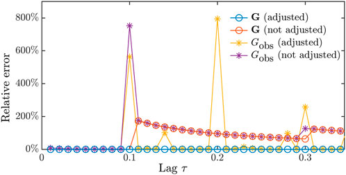
To demonstrate the Nyquist issue, we consider the linear system (Equation 4), where

$\mathbf{A}=\left[\begin{array}{cccc}\hfill -10\hfill & \hfill -100/28\cdot 2\pi \hfill & \hfill 0\hfill & \hfill 0\hfill \\ \hfill 100/28\cdot 2\pi \hfill & \hfill -10\hfill & \hfill 0\hfill & \hfill 0\hfill \\ \hfill 0\hfill & \hfill 0\hfill & \hfill -10\hfill & \hfill -100/20\cdot 2\pi \hfill \\ \hfill 0\hfill & \hfill 0\hfill & \hfill +100/20\cdot 2\pi \hfill & \hfill -10\hfill \end{array}\right],(11)$

$\mathbf{C}=\mathbf{I}$, and $\mathbf{Q}=-(\mathbf{A}+{\mathbf{A}}^T)$. This linear system, similar to example 1 in Penland (2019), consists of two non-interacting rotation submatrices, with the corresponding Nyquist lags being 0.1 and 0.14. We compute the dynamical matrices over different values of $\tau$ using Equations 9a, b under four different conditions: whether the Green function is subjected to residual noise or not and whether the eigen-adjustment is applied or not. Then, the resulting output matrices $A^{\mathrm{o}\mathrm{u}\mathrm{t}\mathrm{p}\mathrm{u}\mathrm{t}}$ are compared with the ground truth matrix $\mathbf{A}$ using the relative error measured by the $L^2$-norm, defined as follows:

$e_{\mathbf{A}}=\frac{{‖A^{\mathrm{o}\mathrm{u}\mathrm{t}\mathrm{p}\mathrm{u}\mathrm{t}}-\mathbf{A}‖}_2}{{‖\mathbf{A}‖}_2}.(12)$

Figure 1 shows the relative errors as a function of $\tau$. Without eigen-adjustment, the relative errors of the estimated dynamical matrices diverge after the smallest Nyquist lag of 0.1, regardless of the presence of residual noise, and do not recover as $\tau$ increases. With eigen-adjustment, the ground truth can be estimated if the Green function is free from noise, which is equivalent to an ideal scenario of flawless and infinite observations. On the other hand, when the noisy Green function is noisy, the Nyquist issue persists at multiples of the Nyquist lags.

Figure 1

Figure 1. Nyquist issue of the ST-LIM. The plot shows the relative errors $e_{\mathbf{A}}$ of the estimated dynamical matrices as a function of lag $\tau$, calculated under four different conditions. $\mathbf{G}$ denotes the theoretical Green function (assumed to be noise-free), and $G^{\mathrm{o}\mathrm{b}\mathrm{s}}$ represents the noisy Green function. In particular, the residual term is set as $r(\tau )=0.01\times e^{-10\tau }N$, where $N$ is a random matrix with entries sampled from the standard Gaussian distribution. The adjusted and non-adjusted conditions show how eigen-adjustment impacts the stability of the estimated dynamics, with peaks indicating instability at the multiples of Nyquist lags.

3 CS-LIM

Although the ST-LIM is effective for stationary observational data, its stationary assumption renders it incapable of capturing the periodic characteristics of cyclostationary data. In the CS-LIM framework, we model the underlying unknown periodic system using the periodic OU process as follows:

$\frac{d}{dt}\mathbf{x}=\mathbf{A}\left(t\right)\mathbf{x}+\sqrt{2\mathbf{Q}\left(t\right)}\mathit{\xi },(13)$

where $\mathbf{A}$ and $\mathbf{Q}$ are periodic dynamical and (positive definite) diffusion matrices, respectively, with the same period. Without loss of generality, we may assume that the period equals 1. The time evolution of the probability distribution is given by Equation 5, with $\mathbf{A}$ and $\mathbf{Q}$ being time-dependent. To achieve a cyclostationary steady state, all Floquet multipliers (i.e., the eigenvalues of the monodromy matrix $\mathbf{M}$) of Equation 13 must have modulus less than 1 (Chicone, 2006; OrtizBeviá, 1997). In the cyclostationary steady state, the covariance function $\mathbf{C}$ can be viewed as a function on the circle $\mathbb{S}$ of perimeter 1, called the phase space, which is parametrized by $\theta$. By naturally identifying $\mathbf{A}$ and $\mathbf{Q}$ with functions on $\mathbb{S}$ through the projection map $\omega :\mathbb{R}\to \mathbb{S}$, the balance equation is now described by the cyclostationary FDR (CS-FDR) as follows:

$\frac{d}{d\theta }\mathbf{C}=\mathbf{A}\left(\theta \right)\mathbf{C}\left(\theta \right)+\mathbf{C}\left(\theta \right){\mathbf{A}}^T\left(\theta \right)+2\mathbf{Q}\left(\theta \right).(14)$

For convenience, we identify the phase variable $\theta$ with the time variable $t$ via $\theta =\omega (t)$ without explicitly stating it when there is no confusion.

In general, since $\mathbf{A}(t)\mathbf{A}(s)\ne \mathbf{A}(s)\mathbf{A}(t)$ for some $t$ and $s$, the monodromy matrix $\mathbf{M}$ and the correlation function $\mathbf{K}(\tau ,\theta )=⟨\mathbf{x}(t+\tau ){\mathbf{x}}^T(t)⟩$ do not admit an explicit expression. To better understand the periodic system, as a heuristic example, let us consider $\mathbf{A}(t)=\left(1+f(t)\right)\bar{\mathbf{A}}$, where $\bar{\mathbf{A}}$ is the mean state and $f(t)$ satisfying ${\int }_0^{1}f(t)dt=0$ describes the variation. In this special case, the monodromy matrix can be explicitly written as $\mathbf{M}=e^{\bar{\mathbf{A}}}$, meaning that stability requires all eigenvalues of $\bar{\mathbf{A}}$ to have negative real parts and that temporary instability is possible as $f(t)$ may take values less than $-1$ at certain times. Moreover, the correlation function can be expressed as $\mathbf{K}(\tau ,\theta )=e^{{\int }_t^{t+\tau }\mathbf{A}({\tau }^{\prime })d{\tau }^{\prime }}\mathbf{C}(t)$, implying that the integrated effect of the dynamical matrices over the current time $t$ and its $\tau$-lag later is considered.

Following the workflow of the ST-LIM, our goal is to express $\mathbf{A}$ in terms of the correlation function $\mathbf{K}$. However, $\mathbf{K}$ is, in general, mathematically intractable, making it difficult to derive a logarithmic-like equation similar to Equation 8. Therefore, an alternative approach is necessary.

3.1 e-CS-LIM

To determine the first-order dynamics, Shin et al. (2021) proposed what we now call the interval-wise Markov approximation, forming the basis of the original CS-LIM and the proposed $e$-CS-LIM. For clarity, we briefly outline this method using an example. Consider a set of observations $\{x(t)\}$ of a physical phenomenon with a diurnal period (1 day), with a sampling interval $\mathrm{\Delta }t$ of 15 min over $L$ days. First, by equi-partitioning the phase space into $M=24$ intervals $I_j$ $(j=1,\dots ,24)$, the data are divided into 24 subsets given by $S_j:=\{x(t)|\omega (t)\in I_j\}$, where the $j$th subset contains data sampled during the $j$th hour of a day. Each $S_j$ presents a similar stage of cyclostationary dependence. For each $j$, we compute the observed correlation function $K_j^{\mathrm{o}\mathrm{b}\mathrm{s}}(\tau )$ for $\tau =0$ and $\tau =m\mathrm{\Delta }t$ using data sampled in the $j$-th hour of a day and $\tau$ minutes later; that is, we compute

$K_j^{\mathrm{o}\mathrm{b}\mathrm{s}}\left(\tau \right)=\frac{{\sum }_{x\left(t\right)\in S_j}x\left(t+\tau \right)x{\left(t\right)}^T}{\left|S_j\right|},(15)$

where $\left|S_j\right|$ denotes the number of observations in $S_j$.

The interval-wise Markov approximation plays a crucial role in estimating the dynamics. The $e$-CS-LIM makes the stationary assumption for each hour and attempts to apply Equation 8 to estimate the dynamics. This extends the Markov approximation across all hours, justifying the term interval-wise Markov approximation. However, in contrast to ST-LIM, which uses all available observations to estimate a single dynamical matrix, the $e$-CS-LIM approach may suffer from insufficient sampling due to equi-partitioning. This may further result in noisy $K^{\mathrm{o}\mathrm{b}\mathrm{s}}$ in the phase direction $j$, potentially requiring a filter to smooth $K^{\mathrm{o}\mathrm{b}\mathrm{s}}$ in $j$ before solving the dynamics. This procedure is known as phase averaging (Shin et al., 2021). Once a suitable $K^{\mathrm{o}\mathrm{b}\mathrm{s}}$ is obtained, Equation 8 is applied for each $j$ to compute the estimated dynamics $A_j^{e-\mathrm{C}\mathrm{S}}$, followed by the CS-FDR (Equation 14) to compute the estimated diffusion matrix $Q_j^{e-\mathrm{C}\mathrm{S}}$ for the $j$th hour. As a result, $e$-CS-LIM formally produces an approximate system of the following form:

$\frac{d}{dt}\mathbf{x}=A^{e-\mathrm{C}\mathrm{S}}\left(t\right)\mathbf{x}+\sqrt{2Q^{e-\mathrm{C}\mathrm{S}}\left(t\right)}\mathit{\xi },(16)$

whose cyclostationary probability distribution $P_{\mathit{st}}^{e-\mathrm{C}\mathrm{S}}$ is Gaussian at each $t$. The original CS-LIM follows the same procedure but differs in the numerical implementation, with its output matrices denoted by $A^{\mathrm{o}-\mathrm{C}\mathrm{S}}$ and $Q^{\mathrm{o}-\mathrm{C}\mathrm{S}}$.

Although the interval-wise Markov approximation works in practice, its validity requires further clarification. Though $\mathbf{K}$ does not have an explicit form in general, its first-order right derivative with respect to the lag variable $\tau$ at the origin satisfies the following equation:

${\left.\frac{\partial }{\partial \tau }\right|}_{\tau =0}\mathbf{K}\left(\tau ,\theta \right)=\mathbf{A}\left(\theta \right)\mathbf{K}\left(0,\theta \right)=\mathbf{A}\left(\theta \right)\mathbf{C}\left(\theta \right).(17)$

Therefore, by integrating with respect to $\tau$, we obtain

$\mathbf{K}\left(\tau ,\theta \right)=e^{\tau \mathbf{A}\left(\theta \right)}\mathbf{C}\left(\theta \right)+o\left(\tau \right)\text{\hspace{0.17em}as\hspace{0.17em}}\tau \to 0,(18)$

which indicates that for each phase $\theta$, the correlation function behaves approximately as an exponential function in the lag variable $\tau$. As a result, applying Equation 8 to each $j$ in $e$-CS-LIM provides a reasonable approximation of the underlying deterministic dynamics as long as there are no abrupt phase-dependent variations in the dynamics of the sampling data $\{x(t)\}$ used in Equation 15. This suggests that $e$-CS-LIM is a hybrid-type model: the dynamics are approximated, while the diffusion process follows an analytic formula. Consequently, it does not analytically reconstruct the periodic linear dynamics and diffusion of the linear stochastic process (Equation 3), as mentioned in Section 1.

From a numerical aspect, the scheme of computing the derivative of observed covariance $d{C}^{\mathrm{o}\mathrm{b}\mathrm{s}}$ and the assignment of time coordinates for $C_j^{\mathrm{o}\mathrm{b}\mathrm{s}}=K_j^{\mathrm{o}\mathrm{b}\mathrm{s}}(0)$, $A_j^{e-\mathrm{C}\mathrm{S}}$, and $Q_j^{e-\mathrm{C}\mathrm{S}}$ remain unspecified at this point. For instance, it is unclear whether $j$th covariance $C_j^{\mathrm{o}\mathrm{b}\mathrm{s}}$ corresponds to $j$ o’clock, $j$:30 or another reference time.

In the $e$-CS-LIM framework, the time coordinate $t_j^C$ for $C_j^{\mathrm{o}\mathrm{b}\mathrm{s}}$ is assigned to the midpoint of the $j$th interval. In contrast, the time coordinate $t_j^A$ for $A_j^{e-\mathrm{C}\mathrm{S}}$ is shifted by half the lag, i.e., $t_j^A=t_j^C+0.5\tau$, since the data at 0-lag and $\tau$-lag are used to compute $K_j^{\mathrm{o}\mathrm{b}\mathrm{s}}$ in Equation 15. In general, after sorting, the distance between $t_j^C$ and $t_j^A$ and the distance between $t_j^A$ and $t_{j+1}^C$ can differ. In this case, the computation of $Q^{e-\mathrm{C}\mathrm{S}}$ requires careful treatment. To address this, for simplicity, we assume $\tau$ to be a multiple of $1/M$ whenever discussing diffusion. This ensures that the time coordinates $t^C=\{t_j^C\}$ and $t^A=\{t_j^A\}$ (after appropriate rearrangement) either coincide or alternate at uniform intervals of distance $1/2M$. Then, we assign the time coordinate $t_j^Q$ for $Q_j^{e-\mathrm{C}\mathrm{S}}$ as $t_j^Q=t_j^A$, and we use the center difference scheme to compute $d{C}^{\mathrm{o}\mathrm{b}\mathrm{s}}$ when $t^C$ and $t^A$ coincide and the forward difference scheme when they alternate.

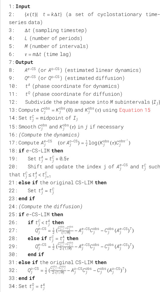
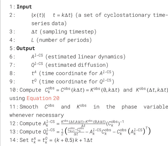
Contrary to the $e$-CS-LIM, the original CS-LIM framework always adopts centered differencing to compute $d{C}^{\mathrm{o}\mathrm{b}\mathrm{s}}$ and a common $j$th time coordinate $t_j$ at the midpoint of the $j$th interval for $C_j^{\mathrm{o}\mathrm{b}\mathrm{s}}$, $A_j^{o-\mathrm{C}\mathrm{S}}$, and $Q_j^{o-\mathrm{C}\mathrm{S}}$. This stencil configuration, however, introduces an artificial phase shift in the estimated dynamics. A schematic illustration and the pseudocode for the original CS-LIM and $e$-CS-LIM are presented in Figure 2 and Algorithm 1, respectively.

Figure 2

Figure 2. Schematic illustration for the $e$-CS-LIM and the original CS-LIM. The circles mark the sampling time of the observational data $\{x(t)\}$ and phase coordinates for covariance $C^{\mathrm{o}\mathrm{b}\mathrm{s}}$ and the dynamical matrices $A^{\mathrm{o}-\mathrm{C}\mathrm{S}}$ for the original CS-LIM and $A^{e-\mathrm{C}\mathrm{S}}$ for the $e$-CS-LIM. The blue shaded areas represent the intervals $I_j$ in the phase space, and the yellow block specifies the sampling used for $x(t+\tau )$ in Equation 15.

3.1.1 Phase shift of the original CS-LIM

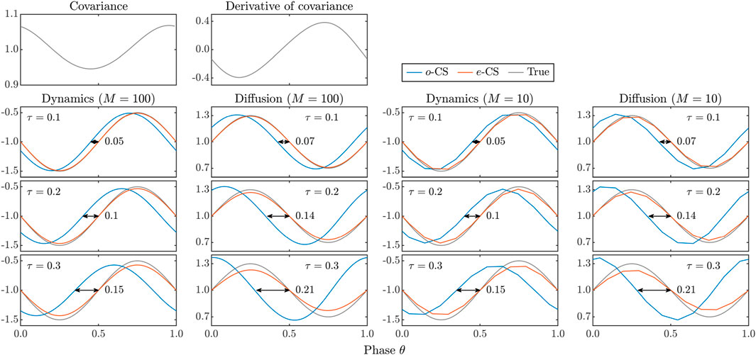
To demonstrate the phase shift, we consider an ideal case in which the observational data $\{x(t)\}$ are sampled using the following equation:

$\frac{d}{dt}\mathbf{x}=-\left(1+f\left(t\right)\right)\bar{\mathbf{A}}\mathbf{x}+\sqrt{2\cdot \left(1+g\left(t\right)\right)\bar{\mathbf{Q}}}\mathit{\xi },(19)$

where $f(t)=0.5\sin (2\pi t)$, $g(t)=0.3\sin (2\pi t)$, $\bar{\mathbf{A}}=-1$, and $\bar{\mathbf{Q}}=1$, over an infinitely long window with a sampling interval $\mathrm{\Delta }t=0.01$. We apply the original CS-LIM and $e$-CS-LIM with $M=100$ (i.e., $K^{\mathrm{o}\mathrm{b}\mathrm{s}}=\mathbf{K}$ on the sample points) and $M=10$. The results are shown in Figure 3.

Figure 3

Figure 3. Phase shift analysis in the original CS-LIM. The upper two subplots show the covariance $\mathbf{C}$ and its derivative $\frac{d}{dt}\mathbf{C}$ of Equation 19. The remaining subplots show the dynamics $\mathbf{A}$ and diffusion $\mathbf{Q}$ (gray) of Equation 19, and the model results obtained using the original CS-LIM (blue) and $e$-CS-LIM (orange) for $M\in \{\mathrm{10,100}\}$ with different lags $\tau \in \{0.1,0.2,0.3\}$. The double-headed arrow in each subplot is the phase difference between the original CS-LIM result and the ground truth, computed by sine wave curve fitting.

Regardless of $M$, the dynamics $A^{\mathrm{o}-\mathrm{C}\mathrm{S}}$ from the original CS-LIM exhibit a notable phase shift of approximately $0.5\mathrm{\Delta }\tau$, which further compromises the accuracy of $Q^{\mathrm{o}-\mathrm{C}\mathrm{S}}$. In contrast, $e$-CS-LIM significantly mitigates the phase shift, even when $\{x(t)\}$ is partitioned into 10 subsets. However, it is worth noting that for a larger $\tau$ value, variations in the dynamics are smoothed out as a consequence of interval-wise Markov approximation and Equation 18. In addition, the Nyquist issue does not arise in the one-dimensional case.

Algorithm 1

Algorithm 1. $e$-CS-LIM (and the original CS-LIM).

3.1.2 Nyquist issue for the e-CS-LIM

Due to the interval-wise application of the ST-LIM, the CS-LIM is also subject to the Nyquist issue. Contrary to the ST-LIM, in which the Nyquist issue does not appear in the theoretical computation when the eigen-adjustment is applied (i.e., $\mathbf{G}$ (adjusted) in Figure 1), the small-o term in Equation 18 introduces a non-trivial residual in Equation 10, causing the Nyquist issue even if flawless infinite observation is possible.

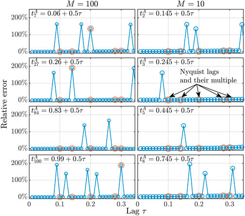
To demonstrate the Nyquist issue, we suppose that the data are sampled infinitely from the periodic linear system (Equation 19), where $f(t)=g(t)=0.5\sin (2\pi t)$, $\bar{\mathbf{A}}$ is given by Equation 11, and $\bar{\mathbf{Q}}=-(\bar{\mathbf{A}}+{\bar{\mathbf{A}}}^T)$. To examine the dependence on the partitioning of the phase space, we consider $M\in \{\mathrm{10,100}\}$ and apply the $e$-CS-LIM over different values of $\tau$.

Figure 4 shows the relative errors between $A_j^{e-\mathrm{C}\mathrm{S}}$ and $\mathbf{A}(t_j^A)$ for certain values of $j$ as a function of $\tau$. Since the dynamical matrix varies in time, the Nyquist issue does not necessarily appear at the multiples of the Nyquist lags of the mean state $\bar{\mathbf{A}}$, but rather near them. In addition, even outside the Nyquist lags, the relative error remains non-zero, which again indicates that the $e$-CS-LIM is not an analytic inverse model for Equation 13. Nevertheless, the relative error is acceptable for application purposes, provided that $\tau$ is not overly large.

Figure 4

Figure 4. Nyquist issue for the $e$-CS-LIM. The relative errors of the output dynamical matrices calculated using Equations 9a, b as a function of the lag variable for distinct $M$. In each subplot, the upper left shows the phase coordinate $t_j^A$ assigned to $A_j^{e-\mathrm{C}\mathrm{S}}$. The orange circles specify the multiples of Nyquist lags of the mean dynamics.

3.2 l-CS-LIM

As the $e$-CS-LIM interval-wise approximates the underlying stochastic process using a Markov system and applies Equation 8, we aim to build an (analytic) inverse model for the periodic Markov system (Equation 3). Instead of using the global information of $\mathbf{K}$ as in the ST-LIM, the $l$-CS-LIM extracts the dynamics by applying Equation 17, the local information of $\mathbf{K}$, followed by computing the diffusion matrix using CS-FDR. This suggests that given the observational data, the $l$-CS-LIM outputs the best-fit periodic Markov system for the unknown complex periodic system, provided that the sampling interval $\mathrm{\Delta }t\ll 1$ and the observation window $L\gg 1$. In practice, the observed correlation function $K^{\mathrm{o}\mathrm{b}\mathrm{s}}$ is obtained using the following equation:

$K^{\mathrm{o}\mathrm{b}\mathrm{s}}\left(\tau ,\theta \right)=\frac{{\sum }_{\omega \left(t\right)=\theta }x\left(t+\tau \right)x{\left(t\right)}^T}{L},(20)$

and the partial derivatives of correlation function ${\partial }_{\tau }{K}^{\mathrm{o}\mathrm{b}\mathrm{s}}$ and ${\partial }_{\theta }{K}^{\mathrm{o}\mathrm{b}\mathrm{s}}$ are estimated by forward finite difference. The corresponding time coordinates for the estimated time-dependent dynamics $A^{l-\mathrm{C}\mathrm{S}}$ and diffusion $Q^{l-\mathrm{C}\mathrm{S}}$ are shifted to the right by $0.5\mathrm{\Delta }t$. In other words, $t^A=t^Q=t^C+0.5\mathrm{\Delta }t$, where $t^A$, $t^Q$, and $t^C$ denote the general reference of the time coordinates for $A^{l-\mathrm{C}\mathrm{S}}$, $Q^{l-\mathrm{C}\mathrm{S}}$, and $C^{\mathrm{o}\mathrm{b}\mathrm{s}}$, respectively, as previously stated. As a result, the $l$-CS-LIM formally determines a periodic linear system as follows:

$\frac{d}{dt}\mathbf{x}=A^{l-\mathrm{C}\mathrm{S}}\left(t\right)\mathbf{x}+\sqrt{2Q^{l-\mathrm{C}\mathrm{S}}\left(t\right)}\mathit{\xi },(21)$

whose cyclostationary distribution $P_{\mathit{st}}^{l-\mathrm{C}\mathrm{S}}$ is also Gaussian for each $t$. The algorithm of $l$-CS-LIM is summarized in Algorithm 2.

This derivative-based method avoids the multi-valued matrix logarithm and is, therefore, not affected by the Nyquist issue. However, it is more sensitive to noise, and phase averaging is applied to $K^{\mathrm{o}\mathrm{b}\mathrm{s}}$ whenever necessary.

3.3 Relationship among LIMs

All LIMs discussed in this article are related. First, we note that the $l$-CS-LIM is indeed an extension of the ST-LIM. If the linear dynamics and diffusion matrix are constant in time, the correlation function is independent of phase variable $\theta$, and Equation 17 can be written in the following form.

Algorithm 2

Algorithm 2.$l$-CS-LIM.

${\left.\frac{d}{d\tau }\right|}_{\tau =0}\mathbf{K}\left(\tau \right)=\mathbf{A}\mathbf{C},(22)$

which is equivalent to the right derivative of Equation 7. At the same time, for a general periodic stochastic process, we can view $l$-CS-LIM as approximating the underlying system using a Markov system at each instant as Equations 17, 22 share the same form. Therefore, we may say that $l$-CS-LIM utilizes the pointwise Markov approximation contrary to the interval-wise version adopted in the $e$-CS-LIM.

A natural question is whether the ST-LIM accurately estimates the mean state $\bar{\mathbf{A}}={\int }_0^1\mathbf{A}(t)dt$ from the infinite cyclostationary observational data sampled from the periodic Markov system (Equation 3). As the correlation function used in the ST-LIM is the integral of $\mathbf{K}(\tau ,\theta )$ over $\theta$, it is clear that it does not equal $e^{\tau \bar{\mathbf{A}}}\bar{\mathbf{C}}$, where $\bar{\mathbf{C}}={\int }_0^1\mathbf{C}(t)dt$ is the mean covariance. Nevertheless, if $\mathbf{A}$ does not vary drastically, the estimated linear dynamics from ST-LIM remain close to the mean state, preserving the dynamics-relevant information of the underlying system.

From a numerical viewpoint, at a given phase $\theta$, the $l$-CS-LIM applies the forward difference method to the observed correlation function $K^{\mathrm{o}\mathrm{b}\mathrm{s}}$ at two consecutive points $\tau =0,\mathrm{\Delta }t$, which amounts to a linear fit of these two points. On the other hand, the $e$-CS-LIM calculates $K^{\mathrm{o}\mathrm{b}\mathrm{s}}$ at the origin and the point at $m\mathrm{\Delta }t$ and applies Equation 8, which corresponds to an exponential curve fitting whenever the Nyquist issue does not persist. This justifies the prefixes $e$-CS-LIM and $l$-CS-LIM. As a result of Equation 18, the $e$-CS-LIM converges to the $l$-CS-LIM under the conditions of $m=1$, $M=\frac{1}{\mathrm{\Delta }t}$, $\mathrm{\Delta }t\ll 1$, and $L\gg 1$. Consequently, the $l$-CS-LIM can be viewed as an instantaneous version of the $e$-CS-LIM.

In practical applications, the difference between the $l$-CS-LIM and $e$-CS-LIM goes beyond the estimation of dynamics. The $l$-CS-LIM, as a derivative-based method, pointwise estimates the Jacobian, which is the first-order approximation of the unknown dynamics. As the state variable moves away from the steady state or as time marches, the higher-order terms in the function’s expansion may become more significant, and the accuracy of linear approximation decreases, lowering the effectiveness of approximating the unknown system using Equation 13. Nevertheless, the Jacobian can still be important in certain practical applications. The $e$-CS-LIM, on the other hand, finds the best-fit linear system within each subinterval in the phase space. Though the $e$-CS-LIM is not an analytic inverse model for a general periodic OU process, it remains effective because for each phase, more sampling can be used in Equation 15 than in Equation 20, and the lag $\tau$ can exceed $\mathrm{\Delta }t$. As a result, the $e$-CS-LIM is more robust to noise than $l$-CS-LIM. The intercomparison among LIMs is summarized in Table 1.

Table 1

Table 1. Intercomparison of linear inverse models.

4 Numerical experiments

As the CS-LIMs compute the dynamical and diffusion matrices using the observed correlation function $K^{\mathrm{o}\mathrm{b}\mathrm{s}}$, they can be regarded as functions that take $K^{\mathrm{o}\mathrm{b}\mathrm{s}}$ as input and produce the estimated dynamics and diffusion. As an inverse method, the accuracy of these estimates depends on the quality of $K^{\mathrm{o}\mathrm{b}\mathrm{s}}$ (Lien et al., 2024). If $K^{\mathrm{o}\mathrm{b}\mathrm{s}}$ computed from observations accurately captures the true correlation function, then both CS-LIMs are expected to effectively estimate both dynamics and diffusion. However, due to the finite number of observations, $K^{\mathrm{o}\mathrm{b}\mathrm{s}}$ is inevitably affected by noise, raising concerns about the stability of the algorithms as numerical derivatives are required. Therefore, in this section, we evaluate the performance and sensitivity of both $e$-CS-LIM and $l$-CS-LIM using the synthetic time-series data $\{x(t)\}$ of Equation 3 under various conditions. For notational convenience, we write $A^{\mathrm{C}\mathrm{S}}$ and $Q^{\mathrm{C}\mathrm{S}}$ as general references for $A^{e-\mathrm{C}\mathrm{S}}$ and $A^{l-\mathrm{C}\mathrm{S}}$ as well as $Q^{e-\mathrm{C}\mathrm{S}}$ and $Q^{l-\mathrm{C}\mathrm{S}}$, respectively.

More precisely, for the given $\mathbf{A}(t)$ and $\mathbf{Q}(t)$, we use the Euler approach with a timestep of $dt=0.002$ from $T_0=0$ to $T_f=L$ to generate auxiliary time-series data; we then subsample it with a sampling step of $\mathrm{\Delta }t$ to obtain the observational data $\{x(t)\}$, and we use CS-LIMs to obtain the estimates $A^{\mathrm{C}\mathrm{S}}$ and $Q^{\mathrm{C}\mathrm{S}}$. As the accuracy of models depends on the stochastic nature of the dataset, the abovementioned process will be repeated 128 times in each scenario, and the resulting statistics (e.g., median) of relative errors, defined similarly to Equation 12, will be used to evaluate the models. This evaluation process will be applied to each case presented in this section.

4.1 One-dimensional case

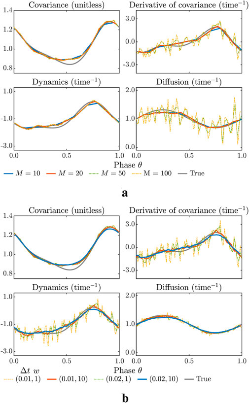
To visualize the CS-LIM results, we start with a one-dimensional case represented by Equation 19, where $f(t)=0.3\pi \sin (2\pi t)+0.1\pi \cos (4\pi t)$, $g(t)=0.1\pi \sin (2\pi t)$, $\bar{\mathbf{A}}=-1$, and $\bar{\mathbf{Q}}=1$. For the $e$-CS-LIM, no filter is applied to the observed correlation function $K^{\mathrm{o}\mathrm{b}\mathrm{s}}$, while for the $l$-CS-LIM, a sliding average with a window of length $w$ is applied to $K^{\mathrm{o}\mathrm{b}\mathrm{s}}$ and $C^{\mathrm{o}\mathrm{b}\mathrm{s}}$.

Figure 5a shows an example of the $e$-CS-LIM results for $T_f=1000$, $\tau =0.1$, and $\mathrm{\Delta }t=0.01$ under a distinct number of intervals $M\in \{\mathrm{10,20,50,100}\}$. Although a smaller $M$ reduces the resolution of the reconstruction, it does not significantly affect the reconstructed dynamics $A^{e-\mathrm{C}\mathrm{S}}$ as long as the variation can be effectively captured by $t^A$. Moreover, a smaller $M$ enhances robustness against noise, leading to a more stable estimate of $Q^{e-\mathrm{C}\mathrm{S}}$. For $M=100$, the stochastic influences in estimated dynamics $A^{e-\mathrm{C}\mathrm{S}}$ remain limited since the lag $\tau =10\mathrm{\Delta }t=0.1$ can be chosen to be larger than $\mathrm{\Delta }t$, thereby mitigating numerical instability associated with dividing noisy data by a small number. This is consistent with the theoretical case illustrated in Figure 3. However, in the computation of $Q^{e-\mathrm{C}\mathrm{S}}$, the numerical differentiation of noisy $C^{\mathrm{o}\mathrm{b}\mathrm{s}}$ results in unfavorable noise amplification in $Q^{e-\mathrm{C}\mathrm{S}}$. Although phase averaging of $C^{\mathrm{o}\mathrm{b}\mathrm{s}}$ could mitigate this issue, we do not pursue this further for $e$-CS-LIM in our analysis.

Figure 5

Figure 5. Examples of CS-LIMs applied to synthetic observational data with $T_f=1000$, $\mathrm{\Delta }t=0.01$, and $\tau =0.1$. (a) Upper panels of each subfigure show true (gray) and numerical (color) covariance and its derivative used in the computation of e-CS-LIM for a distinct number of intervals $M\in \{\mathrm{10,20,50,100}\}$. The true $\mathbf{A}$ and $\mathbf{Q}$ (gray) and the model outputs $A^{e-\mathrm{C}\mathrm{S}}$ and $Q^{e-\mathrm{C}\mathrm{S}}$ (color) are shown in the lower panels. (b) This is analogous to (a) but shows the $l$-CS-LIM result under distinct sampling interval $\mathrm{\Delta }t$ and window length $w$.

Figure 5b shows an example of the $l$-CS-LIM results for $T_f=1000$ under different parameter settings: sampling intervals $\mathrm{\Delta }t\in \{0.01,0.02\}$ and a window width of moving averaging $w\in \{\mathrm{1,10}\}$. Without phase averaging $(w=1)$, noisy $K^{\mathrm{o}\mathrm{b}\mathrm{s}}$ causes amplified noisy variations in $A^{l-\mathrm{C}\mathrm{S}}$, especially for the small sampling interval $\mathrm{\Delta }t=0.01$, raising concerns over whether $A^{l-\mathrm{C}\mathrm{S}}$ contains excessive stochastic influences. This issue can be effectively addressed by applying phase averaging to $K^{\mathrm{o}\mathrm{b}\mathrm{s}}$; when $w=10$, the estimated $A^{l-\mathrm{C}\mathrm{S}}$ provides a clean representation of the underlying dynamics.

In contrast, the estimated $Q^{l-\mathrm{C}\mathrm{S}}$ for $w=1$ appears more robust to the noisy numerical derivatives, though this may be attributed to the idealized nature of synthetic data and the choice of finite difference schemes. To further examine the sensitivity, we introduce artificial perturbations to $K^{\mathrm{o}\mathrm{b}\mathrm{s}}$ by adding a small noise matrix $r$ and apply the resulting correlation function to lines 12 and 13 in Algorithm 2. The corresponding estimated diffusion then exhibits noisy variation, confirming the sensitivity of $Q^{l-\mathrm{C}\mathrm{S}}$ to noisy $K^{\mathrm{o}\mathrm{b}\mathrm{s}}$. Nevertheless, applying phase averaging to the noisy correlation function again effectively removes the undesired noisy variations in the estimates. Finally, it is noted that the CS-FDR is maintained since the filtering is applied to $K^{\mathrm{o}\mathrm{b}\mathrm{s}}$ rather than $A^{l-\mathrm{C}\mathrm{S}}$ or $Q^{l-\mathrm{C}\mathrm{S}}$.

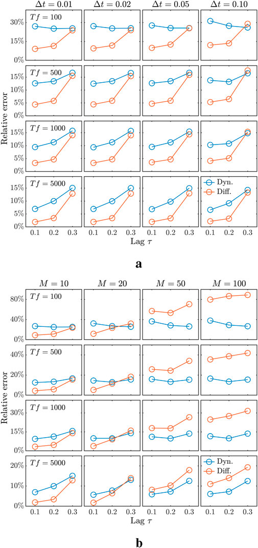
Next, we examine the sensitivity of CS-LIMs to various parameters. Figure 6a shows the results of the $e$-CS-LIM for a fixed $M=10$. As the observation time $T_f$ increases, $K^{\mathrm{o}\mathrm{b}\mathrm{s}}$ more accurately reflects the underlying system, and hence, the performance consistently improves. However, the accuracy decreases with increasing $\tau$ due to its smoothing effect on $A^{e-\mathrm{C}\mathrm{S}}$, which is consistent with the analytic case shown in Figure 3. In addition, reducing $\mathrm{\Delta }t$ leads to a modest performance enhancement for the $e$-CS-LIM since more data points are used in Equation 15, but the improvement is limited.

Figure 6

Figure 6. Performance of $e$-CS-LIM. (a) Each subplot shows the errors with respect to $\tau$ under a fixed M=10 and different values of $\mathrm{\Delta }t$ and $T_f$. (b) Each panel shows the errors with respect to $\tau$ under a fixed Δt = 0.01 and different values of $M$ and $T_f$.

In addition, although the numbers of the observational data for cases $(\mathrm{\Delta }t,T_f)=(0.01,500)$ and $(0.1,5000)$ are the same, their performance differs. This discrepancy arises because in the former case, all observational data corresponding to the subinterval $I_j$ contribute to the computation of $K_j^{\mathrm{o}\mathrm{b}\mathrm{s}}$ and $C_j^{\mathrm{o}\mathrm{b}\mathrm{s}}$, which is equivalent to capturing the integrated effect near $t_j^A$ and $t_j^C$. In contrast, $K_j^{\mathrm{o}\mathrm{b}\mathrm{s}}$ and $C_j^{\mathrm{o}\mathrm{b}\mathrm{s}}$ in the latter are directly at $t_j^A$ and $t_j^C$ since $M=1/\mathrm{\Delta }t$.

Figure 6b shows the results for a fixed $\mathrm{\Delta }t=0.01$ with varying $M\in \{\mathrm{10,20,50,100}\}$. As previously discussed, the noisy variations in $A^{e-\mathrm{C}\mathrm{S}}$ associated with larger $M$ are limited due to a suitable $\tau$. However, the $Q^{e-\mathrm{C}\mathrm{S}}$ remains more sensitive to the noisy numerical derivative of covariance, implying the need for phase averaging. As a result, to optimize the performance of the $e$-CS-LIM, a balance must be struck: $M$ should be kept as small as possible to minimize noise amplification in $Q^{e-\mathrm{C}\mathrm{S}}$, while $\tau$, optimally chosen as $1/M$, should remain small enough to prevent excessive smoothing or insufficient resolution that could obscure meaningful variations in $A^{e-\mathrm{C}\mathrm{S}}$ and $Q^{e-\mathrm{C}\mathrm{S}}$.

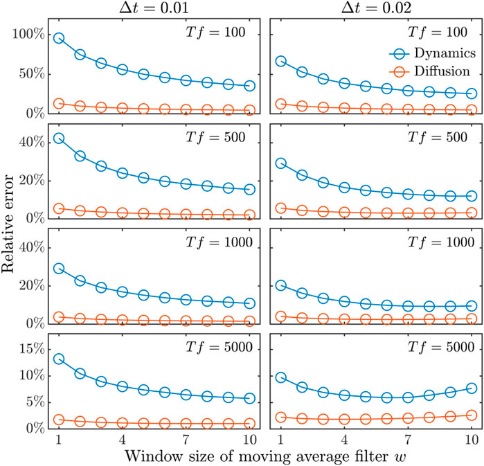
Moreover, we analyze the impact of sampling interval and filtering on the $l$-CS-LIM, as shown in Figure 7. First, we see that if no filter is applied, a larger $\mathrm{\Delta }t$ in the calculation of the numerical derivative, though less accurate in the finite difference approximation, is less sensitive to noise, leading to a lower relative error in the noise-dominant cases. Then, we observe that applying phase averaging to $K^{\mathrm{o}\mathrm{b}\mathrm{s}}$ effectively reduces the noisy variations in $A^{l-\mathrm{C}\mathrm{S}}$, stabilizing the dynamics estimation, particularly at small $T_f$ or small $\mathrm{\Delta }t$, with a clear decrease as window size $w$ increases. However, in cases with limited noisy variations, particularly at large $T_f$ and larger $\mathrm{\Delta }t$, excessive filtering can lead to additional error by overly dampening meaningful fluctuations, which is noticeable in the case of $T_f=5000$ and $\mathrm{\Delta }t=0.02$. Thus, optimal phase averaging requires balancing noise reduction and the preservation of essential variations to prevent over-smoothing, particularly when the noise level is low.

Figure 7

Figure 7. Relative errors of the $l$-CS-LIM. Each panel shows the errors with respect to the window size $w$ for filtering under different values of $\mathrm{\Delta }t$ and $T_f$.

4.2 Higher-dimensional cases

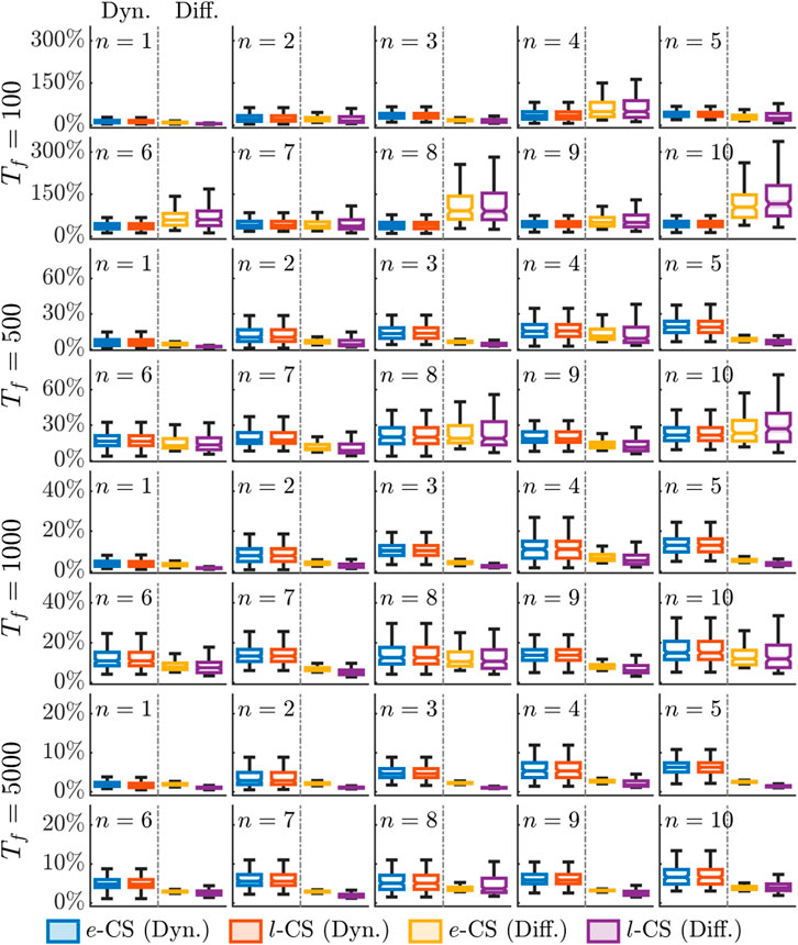
From the previous section, we observed that the lag variable $\tau$ and the number of division $M$ of the phase space play critical roles in the $e$-CS-LIM performance, and filtering with the optimal window size $w$ effectively removes the noisy component and retains the meaningful fluctuation in the $l$-CS-LIM. In this section, we extend the analysis to multi-dimensional cases, setting $\tau =0.1$ and $M=10$ for the $e$-CS-LIM and $w=10$ for the $l$-CS-LIM with a sampling interval $\mathrm{\Delta }t=0.01$. The underlying equation is still represented by Equation 19, with $f(t)$ and $g(t)$ being the same as in the previous section. Each entry of $\bar{\mathbf{A}}$ and $\bar{\mathbf{Q}}$ is initially drawn from the standard normal distribution and then adjusted so that $\bar{\mathbf{A}}$ is a damping operator and $\bar{\mathbf{Q}}$ is positive definite. The Nyquist lag in this setup is significantly larger than $\tau =0.1$, eliminating concerns about the Nyquist issue.

The performance of CS-LIMs across dimension $n$ from 1 to 10 is summarized in Figure 8. In general, if the observation timespan $T_f$ is sufficiently long so that $K^{\mathrm{o}\mathrm{b}\mathrm{s}}$ well-estimates the underlying true correlation function $\mathbf{K}$, both CS-LIMs can effectively capture dynamics and diffusion. Otherwise, the estimation can fail drastically, especially for $Q^{\mathrm{C}\mathrm{S}}$ in higher-dimensional cases, since it is the sum of multiple noisy time series. It should be noted that this study does not aim to compare the two CS-LIM variants directly because the accuracy of CS-LIMs is influenced by numerous factors. For example, the $e$-CS-LIM may struggle to capture fine variations or locate peaks due to its relatively sparse resolution on the phase space, while the $l$-CS-LIM depends on the choice of filtering, and the optimal support or window size of filtering may vary by applications.

Figure 8

Figure 8. Box plots of the relative errors between CS-LIM outputs and the ground truth. Each subplot shows the distribution of relative errors across different dimensions $n$ and observation time spans $T_f$. The box plots show the maximum, minimum, median, and quantiles of the relative errors, with outliers removed. The left half of each subplot corresponds to the relative errors in dynamics while the right half is in diffusion.

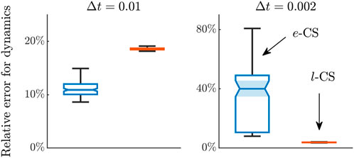
Finally, we revisit the Nyquist issue. We keep the underlying system the same (i.e., $f$ and $g$ remains unchanged) but with $\bar{\mathbf{A}}$ given by Equation 11 and $\bar{\mathbf{Q}}=-(\bar{\mathbf{A}}+{\bar{\mathbf{A}}}^T)$. Figure 9 shows the relative errors in the dynamics for an observation time $T_f=1000$, with parameters $M=10$ and $\tau =0.1$ for the $e$-CS-LIM and $w=10$ when $\mathrm{\Delta }t=0.01$ and $w=50$ when $\mathrm{\Delta }t=0.002$ for the $l$-CS-LIM. The window size $w$ is chosen such that the sliding average filter has a support of 0.1, which is equal to the lag $\tau$ in thed $e$-CS-LIM. At a timestep of $\mathrm{\Delta }t=0.01$, $e$-CS-LIM performance appears stable and reliable, but closer examination reveals that extreme spikes in the estimated dynamics occur randomly but frequently. Unlike the case of the stationary LIM, this error is relatively limited, as only certain points are affected by the Nyquist issue, while others remain accurate. The $l$-CS-LIM result, in contrast, exhibits a narrower error range but overall higher relative errors. When $\mathrm{\Delta }t$ is reduced to 0.002, the sensitivity of the $e$-CS-LIM to the Nyquist issue increases, with relative errors now ranging from 8% to 81%, even exceeding the error range in Figure 8 for $T_f=1000$ and $n=4$, where $\bar{\mathbf{A}}$ and $\bar{\mathbf{Q}}$ are randomly generated. Meanwhile, the $l$-CS-LIM exhibits a stable and narrow error range with significant improvement, implying that the large relative error for the $l$-CS-LIM with $\mathrm{\Delta }t=0.01$ mainly arises from the finite difference scheme used in the computation.

Figure 9

Figure 9. Impact of the Nyquist issue on the numerical computation. Each subplot shows the statistics of the relative errors for dynamics under two different sampling intervals $\mathrm{\Delta }t$. The synthetic sampling datasets are generated with $T_f=1000$. The $e$-CS-LIM estimates dynamics using $M=10$ and $\tau =0.1$, while the $l$-CS-LIM computes dynamics with $w=10$ for $\mathrm{\Delta }t=0.01$ and $w=50$ for $\mathrm{\Delta }t=0.002$. Outliers have been removed.

5 Real-world example: the ENSO recharge oscillator

The El Niño-Southern Oscillation is a dominant interannual climate mode driven by interactions between the ocean and the atmosphere over the tropical Pacific Ocean (Di Lorenzo et al., 2015). The ENSO oscillates between two primary phases, namely, El Niño and La Niña, characterized by unusual warming and cooling of SSTs in the central and eastern Pacific, respectively (Capotondi et al., 2015; Okumura et al., 2011). The Niño 3.4 SST index, defined as the anomaly of the average SST over the region 5S–5N and 170W–120W, serves as a widely used indicator to monitor and predict El Niño and La Niña events (Capotondi et al., 2015; Okumura, 2019).

In climate modeling, the variability in oceanic variables can be viewed as the superposition of atmospheric variability and subsurface processes, modeled by external stochastic forcing and deterministic dynamics, respectively (Deser et al., 2010; Lou et al., 2020). Consequently, ENSO can be viewed as a periodically driven stochastic process. Previous studies have emphasized the seasonal variations in the ENSO (Cane et al., 1986; Chen and Jin, 2021; Chen and Jin, 2022; Levine and McPhaden 2015; Shin et al., 2021; Webster and Yang 1992), but only a few have quantified the relative roles of the seasonal variations in the predictable SST dynamics and unpredictable stochastic forcing (Shin et al., 2021).

In this study, we revisit one of the simplest low-dimensional linear models of the ENSO, which represents the system using the anomalies of area-averaged SSTs and the depth of the 20°C isotherm (D20) over the equatorial Pacific (Burgers et al., 2005; Jin et al., 2007). Under the stationary assumption, previous research has interpreted the ENSO mechanism as a recharge oscillator, where the SST anomaly and D20 anomaly play the roles of momentum and position, respectively (Burgers et al., 2005).

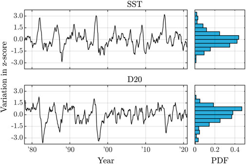
For our analysis, we obtained monthly SST and D20 data from ORAS5 reanalysis for the period 1979–2021 (Zuo et al., 2019). These data were then averaged over 5S–5N and 170W–120W for SSTs and 5S–5N and 120E–80W for D20. Given that the data may exhibit quasi-stationary behavior due to low-frequency signals such as Pacific decadal variability, we applied a linear detrending procedure as a preprocessing step (Kuo et al., 2023). To study the seasonal dependence of the ENSO, we utilized the $l$-CS-LIM and $e$-CS-LIM, applying them to the z-scores of the preprocessed averaged SST and D20 anomalies.

To reduce sampling uncertainties, we also applied a three-month sliding average to $K^{\mathrm{o}\mathrm{b}\mathrm{s}}$ for both CS-LIMs rather than directly smoothing the input data. This approach follows the methodology proposed by Shin et al. (2021). The input data and their distributions are shown in Figure 10.

Figure 10

Figure 10. Observed SST and D20 anomalies in the z-score. The left panels show the time-series of SSTs and D20 from 1979 to 2021, and the right panels show the corresponding probability density functions using histograms.

Using the CS-LIMs, we obtain the time-dependent dynamics $A^{\mathrm{C}\mathrm{S}}$ and diffusion matrices $Q^{\mathrm{C}\mathrm{S}}$. As they are defined at discrete points, we apply linear interpolation entry-wise to construct the approximate systems, as described in Equations 16, 21. The covariance matrices reconstructed by the CS-LIM are calculated from the synthetic data generated from the approximate systems over 5,500 years and are used to estimate the cyclostationary distributions $P_{\mathit{st}}^{l-\mathrm{C}\mathrm{S}}$ and $P_{\mathit{st}}^{e-\mathrm{C}\mathrm{S}}$ (collectively referred to as $P_{\mathit{st}}^{\mathrm{C}\mathrm{S}}$).

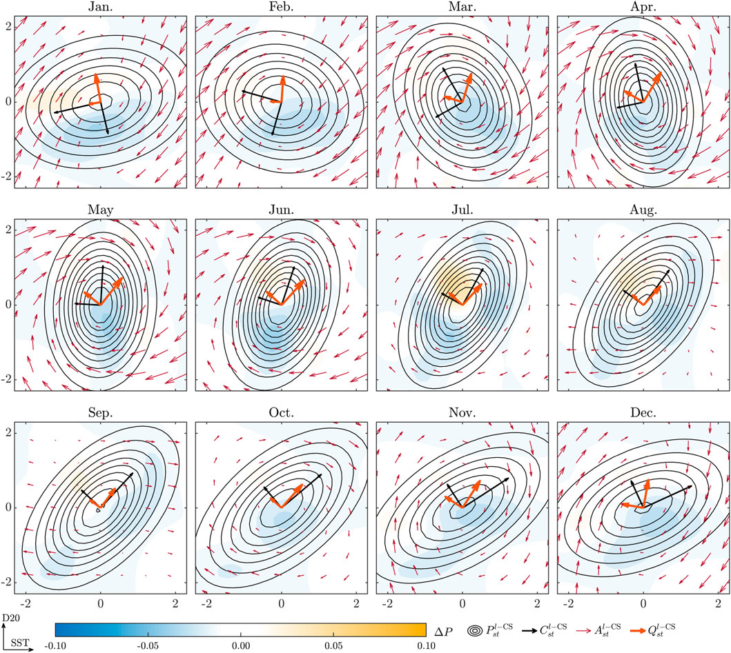
To compare $P_{\mathit{st}}^{\mathrm{C}\mathrm{S}}$ with observations, we apply the bivariate Gaussian kernel density estimator to calculate the observed joint probability density function (PDF) $P_{\mathit{st}}^{\mathrm{o}\mathrm{b}\mathrm{s}}$ for each calendar month. Figures 11, 12 show the cyclostationary distributions $P_{\mathit{st}}^{\mathrm{C}\mathrm{S}}$, the vector fields associated with the dynamics $A^{\mathrm{C}\mathrm{S}}$, and eigenvectors of $Q^{\mathrm{C}\mathrm{S}}$ scaled by the square root of the corresponding eigenvalues to represent the approximate periodic Markov systems.

Figure 11

Figure 11. $l$-CS-LIM result on the normalized coordinate. The $x$-and $y$-axes represent the z-scores of SST and D20 anomalies, respectively. The cyclostationary distribution $P_{\mathit{st}}^{l-\mathrm{C}\mathrm{S}}$ is represented by the black contour lines, with the black arrows indicating the eigenvectors of the covariance matrix scaled by the square root of the corresponding eigenvalues. The quiver plot shows the vector fields of the estimated first-order dynamics, while the thick orange arrows are the eigenvectors of the diffusion matrix scaled by the square root of the corresponding eigenvalues. The filled contours show the difference between the theoretical $P_{\mathit{st}}^{l-\mathrm{C}\mathrm{S}}$ and the observed $P_{\mathit{st}}^{\mathrm{o}\mathrm{b}\mathrm{s}}$, with colors ranging from $-0.10$ to 0.10.

Figure 12

Figure 12. $e$-CS-LIM result on the normalized coordinate plane. This figure is analogous to Figure 11, but the results are based on the $e$-CS-LIM. See Figure 11 for a detailed description of the elements displayed.

The results reveal that the estimated dynamics exhibit a clockwise spiral sink for most calendar months, contributing to a rotational pattern in the cyclostationary distribution, except in late August and September. In addition, the principal direction of the diffusion matrices consistently remains in the first quadrant throughout the year, indicating that atmospheric stochastic forcing mainly acts to warm or cool both the surface and sublayer at the same time. The discrepancy $\mathrm{\Delta }P:=P_{\mathit{st}}^{\mathrm{o}\mathrm{b}\mathrm{s}}-P_{\mathit{st}}^{\mathrm{C}\mathrm{S}}$, shown by the filled contours in Figures 11, 12, predominantly appears negative on the upper plane but positive on the lower plane throughout the year. This tendency can be mainly attributed to the negative skewness in the z-score of the D20 anomaly shown in Figure 10 as the approximate systems yield a time-dependent Gaussian distribution $P_{\mathit{st}}^{\mathrm{C}\mathrm{S}}$.

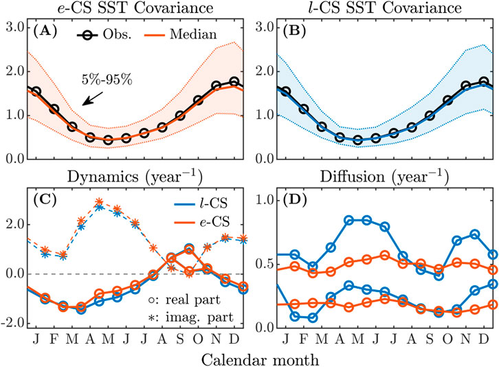
Figure 13 shows the seasonal variation in the eigenvalues of $A^{\mathrm{C}\mathrm{S}}$ and $Q^{\mathrm{C}\mathrm{S}}$. The results for the deterministic dynamics from both CS-LIMs are consistent, showing a notable seasonal dependence; although the dynamics overall act as a damping force, they become temporarily unstable in boreal fall. The imaginary part is especially prominent in boreal late spring and summer, contributing to a phase transition in the SST–D20 correlation that shifts from negative to positive. However, in boreal autumn, the dynamics slow down significantly, and two real eigenvalues even appear in October, indicating a non-rotating regime. The Floquet exponents (i.e., the principal logarithms of the Floquet multipliers) of the approximate system determined by the $l$-CS-LIM and $e$-CS-LIM reveal decay rates of 2.01 and 2.41 years with periods of 4.05 and 3.83 years, respectively. These are slightly different from, but consistent with, the ST-LIM result with a decay rate of 2.00 years and a period of 3.08 years (Burgers et al., 2005).

Figure 13

Figure 13. CS-LIM results for the ENSO study. (A, B) The unfiltered observed SST covariance (black), the median (solid), and the 90% confidence levels (shaded area) in the z-score determined by the CS-LIM ensembles. (C) Real (circle) and imaginary (star) parts of the seasonal-dependent eigenvalues of $A^{\mathrm{C}\mathrm{S}}$. (D) Two positive seasonal-dependent eigenvalues of $Q^{\mathrm{C}\mathrm{S}}$. The x-ticks represent the 15th of each calendar month. Notably, in (C, D), the markers and x-ticks alternate.

The diffusion terms reveal distinct seasonal patterns between the two methods. The $e$-CS-LIM shows a minimal seasonal variation in diffusion, whereas the $l$-CS-LIM suggests that the random forcing intensifies in two main periods, namely, April to June and October to November. These contrasting seasonal patterns in diffusion may lead to different interpretations of the ENSO mechanism.

The $l$-CS-LIM result suggests a recurring annual cycle in both oceanic deterministic dynamics and atmospheric stochastic forcing. In March and April, while the background oceanic system pulls the SST and D20 back to equilibrium, the unpredictable atmospheric system intends to determine the ENSO phase (either positive, negative, or neutral) of the upcoming year. Once the phase is established in boreal summer, the oceanic system then acts as a driving force to build up the SST anomaly from August to late October. As the atmospheric forcing intensifies in the following months, the SST anomaly can reach extreme levels—either high or low—from November to January, potentially causing the El Niño and La Niña events. As the cycle progresses, weaker atmospheric excitation and stronger oceanic damping from February and April work help store the SST anomaly, gradually returning the system to its equilibrium state.

It is also noteworthy that the time-dependent stochastic forcing also affects the transition of the SST–D20 correlation. Compared with the case where $Q^{l-\mathrm{C}\mathrm{S}}$ is replaced by the time-independent $\overline{Q^{l-\mathrm{C}\mathrm{S}}}$, the seasonality further speeds up the rotation in $P_{\mathit{st}}^{l-\mathrm{C}\mathrm{S}}$ from April to June since the principal direction of the covariance matrix rotates toward that of the diffusion matrix, whose intensity reaches the maximum over these months. Though the dynamics play a major role in the transition, the seasonal feature of diffusion is not negligible.

Overall, this recurring annual pattern demonstrates how random forcing drives the system away from its mean state, contributing to the inter-annual variability observed in the ENSO. The combination of lower SST anomalies in March and April, along with stronger atmospheric forcing, makes it challenging to predict whether SST anomalies will increase or decrease in the subsequent months, which is a factor potentially linked to the well-known ENSO prediction barrier (Cane et al., 1986; Levine and McPhaden, 2015; Webster and Yang, 1992). Moreover, the unstable deterministic dynamics and enhanced random forcing in boreal autumn may help explain the increased SST variability in boreal winter, contributing to the observed ENSO phase locking (Chen and Jin, 2021; Chen and Jin, 2022).

In contrast, the nearly constant random forcing in the $e$-CS-LIM results may imply that the seasonal variability of the SST anomaly is mainly driven by the seasonal variation in deterministic oceanic dynamics rather than that in the atmospheric excitation force. Compared with the $l$-CS-LIM, we can say that the seasonal feature of $Q^{e-\mathrm{C}\mathrm{S}}$ (if any) is transferred to that of $A^{e-\mathrm{C}\mathrm{S}}$ because the CS-FDR holds in both the methods.

For each model, we generate a 128-member ensemble of 43 years for SST and D20 anomalies by numerically integrating the system (Equation 13) determined by CS-LIMs with a timestep of $dt=0.001$ years. The 90% confidence interval levels of the SST covariance derived from the ensembles are shown in Figure 13. The $l$-CS-LIM result shows wider confidence intervals than the $e$-CS-LIM results from April to June and October to November due to stronger random forcing during these periods. Despite different interpretations of the seasonality of stochastic forcing, both models capture the seasonal variation in observed SST covariance (without smoothing). Moreover, the reconstructed monthly SST–D20 cross-covariances, D20–D20 auto-covariances, and annual correlation functions, shown in Supplementary Material, are consistent with observations, demonstrating their effectiveness in capturing the dominant modes of a non-linear system. Although this is a simplified model for ENSO studies, we emphasize that CS-LIMs can be applied to higher-dimensional climate variables, offering spatial–temporal coherence in complex systems (Kido et al., 2023; Shin et al., 2021).

6 Conclusion

In this article, we examine the mathematical background of CS-LIMs, a class of data-driven methods that construct periodic OU processes from finite cyclostationary data and present the $e$-CS-LIM and $l$-CS-LIM. The $e$-CS-LIM is developed based on interval-wise approximation, dividing the phase space into intervals where data exhibit similar cyclostationary dependencies. This approach enables the ST-LIM to estimate the linear dynamics by capturing the integrated effect over each interval, making it effective for most applications. In addition, the improved stencil design in the $e$-CS-LIM eliminates the phase shift observed in the original CS-LIM. However, despite these improvements, it remains vulnerable to the Nyquist issue, which also affects the ST-LIM. In contrast, the $l$-CS-LIM serves as an analytic inverse model to the periodic OU process and estimates the time-dependent Jacobian of a complex system in general. As a derivative-based method, it inherently avoids the Nyquist issue, offering an alternative for studying periodic systems.

Numerical experiments on synthetic data show that both CS-LIM variants effectively capture the temporal structure of the underlying periodic systems. With an optimally chosen interval division, the $e$-CS-LIM uses a relatively sufficient amount of data to estimate the dynamics and preserves meaningful variations without amplifying noise or excessive smoothing. On the other hand, although the $l$-CS-LIM is sensitive to noise, its performance significantly improves when optimal phase averaging is applied to the observed correlation function. In cases where the Nyquist lag of the mean dynamics is close to the optimal range of $\tau$, the $e$-CS-LIM estimation may fail at certain intervals, leading to significant and abrupt derivations from the underlying system. In contrast, the $l$-CS-LIM remains robust, provided that the sampling interval is sufficiently small to ensure accurate finite difference calculations.

We have applied the CS-LIMs to the real-world Niño SST 3.4 index and the area-averaged depth of $20°$C isotherm, two oceanic variables commonly used to study the ENSO. Our findings show that in the boreal spring, the strong damping dynamics and stochastic forcing associated with the ENSO make deterministic forecasting challenging, which is related to the ENSO prediction barrier. In autumn, the unstable dynamics amplify the SST anomaly established in summer, increasing the SST variability and covariance in winter and potentially contributing to ENSO phase locking. Moreover, the estimated decay rates and periods obtained by both methods align with the current understanding of the ENSO, and the reproduced SST covariance captures observed seasonal dependency. This ENSO study demonstrates the capabilities of CS-LIMs and highlights their potential to provide a deeper insight into complex climate systems.

In addition to time-series analysis, CS-LIMs can also serve as predictive tools for periodic systems (Shin et al., 2021; Vimont et al., 2022). While the ST-LIM has been used for forecasting, particularly in climate science, recent studies have recognized the importance of accounting for seasonality in predictive models (Alexander et al., 2008; Vimont et al., 2022; Zhao et al., 2024). A valuable direction for future research would be a comparative study evaluating how different assumptions in LIMs affect model prediction skills and how they perform relative to AI-based forecasting methods and full dynamical models. Such a comparison would provide key insights into the strengths and limitations of CS-LIMs and help identify the fundamental elements of model predictability.

Moreover, the CS-LIM framework has broad applicability beyond analysis and prediction. Dynamical mode decomposition, the deterministic counterpart of the ST-LIM, has been widely applied to study chaotic and quasi-cyclostationary systems, integrated with wavelet decomposition, and applied to enhance machine learning techniques (Donge et al., 2023; Hou et al., 2025; Krishnan et al., 2023; Kutz et al., 2016; Naderi et al., 2019; Tu et al., 2014). By building on these ideas, CS-LIMs, as periodic extensions of the ST-LIM, have the potential to improve these applications by explicitly incorporating periodic features into system dynamics. We believe that both $e$-CS-LIM and $l$-CS-LIM will offer new perspectives and advancements in climate sciences and other fields of study.

Data availability statement

The raw data supporting the conclusions of this article will be made available by the authors, without undue reservation.

Author contributions

JL: conceptualization, formal analysis, methodology, software, and writing–original draft. Y-NK: conceptualization and writing–review and editing. HA: funding acquisition, supervision, and writing–review and editing. SK: investigation and writing–review and editing.

Funding

The author(s) declare that financial support was received for the research and/or publication of this article. This work was supported by the (1) Council for Science, Technology, and Innovation (CSTI), the Cross-ministerial Strategic Innovation Promotion Program (SIP), and the 3rd period of SIP “Smart energy management system” grant number JPJ012207 (funding agency: JST) and (2) Grant-in-Aid for Scientific Research (B), 23K25946.

Conflict of interest

The authors declare that the research was conducted in the absence of any commercial or financial relationships that could be construed as a potential conflict of interest.

Generative AI statement

The author(s) declare that Generative AI was used in the creation of this manuscript. During the preparation of this manuscript, the authors used ChatGPT-4o in order to improve readability. After using this tool, the authors reviewed and edited the content as needed and took full responsibility for the content of the publication.

Publisher’s note

All claims expressed in this article are solely those of the authors and do not necessarily represent those of their affiliated organizations, or those of the publisher, the editors and the reviewers. Any product that may be evaluated in this article, or claim that may be made by its manufacturer, is not guaranteed or endorsed by the publisher.

Supplementary Material

The Supplementary Material for this article can be found online at: https://www.frontiersin.org/articles/10.3389/fcpxs.2025.1563687/full#supplementary-material

References

Alexander, M. A., Matrosova, L., Penland, C., Scott, J. D., and Chang, P. (2008). Forecasting pacific SSTs: linear inverse model predictions of the PDO. J. Clim. 21, 385–402. doi:10.1175/2007JCLI1849.1

CrossRef Full Text | Google Scholar

Burgers, G., Jin, F.-F., and van Oldenborgh, G. J. (2005). The simplest ENSO recharge oscillator. Geophys. Res. Lett. 32. doi:10.1029/2005GL022951

CrossRef Full Text | Google Scholar

Cane, M. A., Zebiak, S. E., and Dolan, S. C. (1986). Experimental forecasts of El Niño. Nature 321, 827–832. doi:10.1038/321827a0

CrossRef Full Text | Google Scholar

Capotondi, A., Wittenberg, A. T., Newman, M., Di Lorenzo, E., Yu, J.-Y., Braconnot, P., et al. (2015). Understanding ENSO diversity. Bull. Am. Meteorological Soc. 96, 921–938. doi:10.1175/bams-d-13-00117.1

CrossRef Full Text | Google Scholar

Chen, H.-C., and Jin, F.-F. (2021). Simulations of ENSO phase-locking in CMIP5 and CMIP6. J. Clim. 34, 5135–5149. doi:10.1175/JCLI-D-20-0874.1

CrossRef Full Text | Google Scholar

Chen, H.-C., and Jin, F.-F. (2022). Dynamics of ENSO phase-locking and its biases in climate models. Geophys. Res. Lett. 49, e2021GL097603. doi:10.1029/2021GL097603

CrossRef Full Text | Google Scholar

Chicone, C. (2006). “Ordinary differential equations with applications,” in Texts in applied mathematics. New York: Springer.

Google Scholar

Culver, W. J. (1966). On the existence and uniqueness of the real logarithm of a matrix. Proc. Am. Math. Soc. 17, 1146–1151. doi:10.1090/s0002-9939-1966-0202740-6

CrossRef Full Text | Google Scholar

Deser, C., Alexander, M. A., Xie, S.-P., and Phillips, A. S. (2010). Sea surface temperature variability: patterns and mechanisms. Annu. Rev. Mar. Sci. 2, 115–143. doi:10.1146/annurev-marine-120408-151453

PubMed Abstract | CrossRef Full Text | Google Scholar

Di Lorenzo, E., Liguori, G., Schneider, N., Furtado, J. C., Anderson, B. T., and Alexander, M. A. (2015). ENSO and meridional modes: a null hypothesis for pacific climate variability. Geophys. Res. Lett. 42, 9440–9448. doi:10.1002/2015GL066281

CrossRef Full Text | Google Scholar

Donge, V. S., Lian, B., Lewis, F. L., and Davoudi, A. (2023). Accelerated reinforcement learning via dynamic mode decomposition. IEEE Trans. Control Netw. Syst. 10, 2022–2034. doi:10.1109/TCNS.2023.3259060

CrossRef Full Text | Google Scholar

Hamlington, B. D., Leben, R. R., Nerem, R. S., Han, W., and Kim, K.-Y. (2011). Reconstructing sea level using cyclostationary empirical orthogonal functions. J. Geophys. Res. 116, C12015. doi:10.102910.1029/2011jc0075292011JC007529

CrossRef Full Text | Google Scholar

Hou, Y., Chen, J., Ma, D., and Chan, P. W. (2025). Steady-state linear response matrix of the lorenz-63 system. Authorea Preprints.

Google Scholar

H Tu, J., W Rowley, C., M Luchtenburg, D., L Brunton, S., and Nathan Kutz, J. (2014). On dynamic mode decomposition: theory and applications. J. Comput. Dyn. 1, 391–421. doi:10.3934/jcd.2014.1.391

CrossRef Full Text | Google Scholar

Jacka, S. D., and Oksendal, B. (1987). Stochastic differential equations: an introduction with applications. J. Am. Stat. Assoc. 82, 948. doi:10.2307/2288814

CrossRef Full Text | Google Scholar

Jin, F.-F., Lin, L., Timmermann, A., and Zhao, J. (2007). Ensemble-mean dynamics of the ENSO recharge oscillator under state-dependent stochastic forcing. Geophys. Res. Lett. 34. doi:10.1029/2006GL027372

CrossRef Full Text | Google Scholar

Johnson, S. D., Battisti, D. S., and Sarachik, E. S. (2000a). Empirically derived markov models and prediction of tropical pacific sea surface temperature anomalies. J. Clim. 13, 3–17. doi:10.1175/1520-0442(2000)013<0003:edmmap>2.0.co;2

CrossRef Full Text | Google Scholar

Johnson, S. D., Battisti, D. S., and Sarachik, E. S. (2000b). Seasonality in an empirically derived markov model of tropical pacific sea surface temperature anomalies. J. Clim. 13, 3327–3335. doi:10.1175/1520-0442(2000)013<3327:siaedm>2.0.co;2

CrossRef Full Text | Google Scholar

Kido, S., Richter, I., Tozuka, T., and Chang, P. (2023). Understanding the interplay between ENSO and related tropical SST variability using linear inverse models. Clim. Dyn. 61, 1029–1048. doi:10.1007/s00382-022-06484-x

CrossRef Full Text | Google Scholar

Kim, K.-Y. (2002). Investigation of ENSO variability using cyclostationary EOFs of observational data. Meteorology Atmos. Phys. 81, 149–168. doi:10.1007/s00703-002-0549-7

CrossRef Full Text | Google Scholar

Kim, K.-Y., Hamlington, B., and Na, H. (2015). Theoretical foundation of cyclostationary EOF analysis for geophysical and climatic variables: concepts and examples. Earth-Science Rev. 150, 201–218. doi:10.1016/j.earscirev.2015.06.003

CrossRef Full Text | Google Scholar

Krishnan, M., Gugercin, S., and Tarazaga, P. A. (2023). A wavelet-based dynamic mode decomposition for modeling mechanical systems from partial observations. Mech. Syst. Signal Process. 187, 109919. doi:10.1016/j.ymssp.2022.109919

CrossRef Full Text | Google Scholar

Kuo, Y.-N., Kim, H., and Lehner, F. (2023). Anthropogenic aerosols contribute to the recent decline in precipitation over the u.s. southwest. Geophys. Res. Lett. 50, e2023GL105389. doi:10.1029/2023gl105389

CrossRef Full Text | Google Scholar

Kutz, J. N., Brunton, S. L., Brunton, B. W., and Proctor, J. L. (2016). Dynamic mode decomposition. Philadelphia, PA: Society for Industrial and Applied Mathematics.

Google Scholar

Kwasniok, F. (2022). Linear inverse modeling of large-scale atmospheric flow using optimal mode decomposition. J. Atmos. Sci. 79, 2181–2204. doi:10.1175/JAS-D-21-0193.1

CrossRef Full Text | Google Scholar

Levine, A. F. Z., and McPhaden, M. J. (2015). The annual cycle in ENSO growth rate as a cause of the spring predictability barrier. Geophys. Res. Lett. 42, 5034–5041. doi:10.1002/2015GL064309

CrossRef Full Text | Google Scholar

Lien, J., Kuo, Y.-N., Ando, H., and Kido, S. (2025). Colored linear inverse model: A data-driven method for studying dynamical systems with temporally correlated stochasticity. Physical Review Research.

Google Scholar

Lou, J., Holbrook, N. J., and O’Kane, T. J. (2020). A linear inverse model of tropical and south pacific seasonal predictability Url: Available online at: https://presentations.copernicus.org/EGU2020/EGU2020-2235_presentation.pdf.

Google Scholar

Naderi, M. H., Eivazi, H., and Esfahanian, V. (2019). New method for dynamic mode decomposition of flows over moving structures based on machine learning (hybrid dynamic mode decomposition). Phys. Fluids 31, 127102. doi:10.1063/1.5128341

CrossRef Full Text | Google Scholar

Newman, M., Alexander, M. A., and Scott, J. D. (2011a). An empirical model of tropical ocean dynamics. Clim. Dyn. 37, 1823–1841. doi:10.1007/s00382-011-1034-0

CrossRef Full Text | Google Scholar

Newman, M., Shin, S.-I., and Alexander, M. A. (2011b). Natural variation in ENSO flavors. Geophys. Res. Lett. 38. doi:10.1029/2011GL047658

CrossRef Full Text | Google Scholar

Okumura, Y. M. (2019). ENSO diversity from an atmospheric perspective. Curr. Clim. Change Rep. 5, 245–257. doi:10.1007/s40641-019-00138-7

CrossRef Full Text | Google Scholar

Okumura, Y. M., Ohba, M., Deser, C., and Ueda, H. (2011). A proposed mechanism for the asymmetric duration of El Niño and La Niña. J. Clim. 24, 3822–3829. doi:10.1175/2011JCLI3999.1

CrossRef Full Text | Google Scholar

OrtizBeviá, M. J. (1997). Estimation of the cyclostationary dependence in geophysical data fields. J. Geophys. Res. Atmos. 102, 13473–13486. doi:10.1029/97JD00243

CrossRef Full Text | Google Scholar

Penland, C. (1989). Random forcing and forecasting using principal oscillation pattern analysis. Mon. Weather Rev. 117, 2165–2185. doi:10.1175/1520-0493(1989)117<2165:rfafup>2.0.co;2

CrossRef Full Text | Google Scholar

Penland, C. (1996). A stochastic model of IndoPacific sea surface temperature anomalies. Phys. D. Nonlinear Phenom. 98, 534–558. doi:10.1016/0167-2789(96)00124-8

CrossRef Full Text | Google Scholar

Penland, C. (2019). The Nyquist issue in linear inverse modeling. Mon. Weather Rev. 147, 1341–1349. doi:10.1175/.MWR-D-18-0104.1

CrossRef Full Text | Google Scholar

Penland, C., and Magorian, T. (1993). Prediction of Niño 3 sea surface temperatures using linear inverse modeling. J. Clim. 6, 1067–1076. doi:10.1175/1520-0442(1993)006<1067:ponsst>2.0.co;2

CrossRef Full Text | Google Scholar

Penland, C., and Matrosova, L. (1994). A balance condition for stochastic numerical models with application to the El niño-southern oscillation. J. Clim. 7, 1352–1372. doi:10.1175/1520-0442(1994)007<1352:abcfsn>2.0.co;2

CrossRef Full Text | Google Scholar

Penland, C., and Matrosova, L. (2006). Studies of El Niño and interdecadal variability in tropical sea surface temperatures using a nonnormal filter. J. Clim. 19, 5796–5815. doi:10.1175/JCLI3951.1

CrossRef Full Text | Google Scholar

Penland, C., and Sardeshmukh, P. D. (1995). The optimal growth of tropical sea surface temperature anomalies. J. Clim. 8, 1999–2024. doi:10.1175/1520-0442(1995)008<1999:togots>2.0.co;2

CrossRef Full Text | Google Scholar

Perkins, W. A., and Hakim, G. (2020). Linear inverse modeling for coupled atmosphere-ocean ensemble climate prediction. J. Adv. Model. Earth Syst. 12, e2019MS001778. doi:10.1029/2019MS001778

CrossRef Full Text | Google Scholar

Risken, H. (1989). “The Fokker-Planck equation,” in Methods of solution and applications, vol. 18 (Springer-Verlag, Berlin).

Google Scholar

Rüschendorf, L. (2023). “Stochastic processes and financial mathematics,” in Mathematics study resources. Springer Berlin Heidelberg.

Google Scholar

Särkkä, S., and Solin, A. (2019). “Applied stochastic differential equations,” in Institute of mathematical statistics textbooks. Cambridge University Press.

Google Scholar

Seifert, U. (2012). Stochastic thermodynamics, fluctuation theorems and molecular machines. Rep. Prog. Phys. 75, 126001. doi:10.1088/0034-4885/75/12/126001

PubMed Abstract | CrossRef Full Text | Google Scholar

Shin, S.-I., Sardeshmukh, P. D., Newman, M., Penland, C., and Alexander, M. A. (2021). Impact of annual cycle on ENSO variability and predictability. J. Clim. 34, 171–193. doi:10.1175/JCLI-D-20-0291.1

CrossRef Full Text | Google Scholar

Stuecker, M. F. (2023). The climate variability trio: stochastic fluctuations, El Niño, and the seasonal cycle. Geosci. Lett. 10, 51. doi:10.1186/s40562-023-00305-7

CrossRef Full Text | Google Scholar

Stuecker, M. F., Jin, F.-F., Timmermann, A., and McGregor, S. (2015). Combination mode dynamics of the anomalous northwest pacific anticyclone. J. Clim. 28, 1093–1111. doi:10.1175/JCLI-D-14-00225.1

CrossRef Full Text | Google Scholar

Stuecker, M. F., Timmermann, A., Jin, F.-F., McGregor, S., and Ren, H.-L. (2013). A combination mode of the annual cycle and the El Niño/Southern Oscillation. Nat. Geosci. 6, 540–544. doi:10.1038/ngeo1826

CrossRef Full Text | Google Scholar

Vimont, D. J., Newman, M., Battisti, D. S., and Shin, S.-I. (2022). The role of seasonality and the ENSO mode in central and east pacific ENSO growth and evolution. J. Clim. 35, 3195–3209. doi:10.1175/JCLI-D-21-0599.1

CrossRef Full Text | Google Scholar

Webster, P. J., and Yang, S. (1992). Monsoon and ENSO: selectively interactive systems. Q. J. R. Meteorological Soc. 118, 877–926. doi:10.1002/qj.49711850705

CrossRef Full Text | Google Scholar

Xue, Y., Leetmaa, A., and Ji, M. (2000). ENSO prediction with markov models: the impact of sea level. J. Clim. 13, 849–871. doi:10.1175/1520-0442(2000)013<0849:epwmmt>2.0.co;2

CrossRef Full Text | Google Scholar

Zhao, S., Jin, F.-F., Stuecker, M. F., Thompson, P. R., Kug, J.-S., McPhaden, M. J., et al. (2024). Explainable El Niño predictability from climate mode interactions. Nature 630, 891–898. doi:10.1038/s41586-024-07534-6

PubMed Abstract | CrossRef Full Text | Google Scholar

Zuo, H., Balmaseda, M. A., Tietsche, S., Mogensen, K., and Mayer, M. (2019). The ECMWF operational ensemble reanalysis–analysis system for ocean and sea ice: a description of the system and assessment. Ocean Sci. 15, 779–808. doi:10.5194/os-15-779-2019

CrossRef Full Text | Google Scholar