Spectrum optimization of dynamic networks for reduction of vulnerability against adversarial resonance attacks

Resonance is a well-known phenomenon that happens in systems with second order dynamics. In this paper, we address the fundamental question of making a network robust to signal being periodically pumped into it at or near a resonant frequency by an adversarial agent with the aim of saturating the network with the signal. Toward this goal, we develop the notion of network vulnerability, which is measured by the expected resonance amplitude on the network under a stochastically modeled adversarial attack. Assuming a second order dynamics model based on the network graph Laplacian and a known stochastic model for the adversarial attack, we propose two methods for minimizing the network vulnerability–one through direct optimization of the spectrum of the network graph, and another through optimization of an auxiliary network graph attached to the main network. We provide theoretical foundations for these methods as well as extensive numerical results analyzing the effectiveness of both methods in reducing the network vulnerability.

1 Introduction

In this paper we consider the phenomenon of runaway amplification of signal in a network due to resonance, which has implications on security of the network. This is possible if an adversarial agent pumps signal into one or more vertices of the network in a periodic manner at a frequency that matches or is very close to one of the natural frequencies of the network. This phenomenon is observed in networks with a second order signal dynamics.

While second order dynamics over networks has been studied in the past van der Schaft and Maschke (2013), Chow and Kokotovic (1985), Romeres et al. (2013), Cheng et al. (2017), especially in context of power grids (since power transmission using alternating currents are described naturally using second-order dynamics), existing literature does not focus on controlling network parameters and topology for the purpose of mitigation of resonance.

The contributions of this paper are as follows.

• We develop a second-order dynamics model (represented by a system of second order differential equations) for signal transmission over a network under external forcing (source of the adversarial signal), that is consistent with the network topology (Section 3).

• We develop the notion of network vulnerability, measured by the expected resonance amplitude under stochastically modeled adversarial forcing (Section 3).

• We propose two methods, namely, Network Graph Optimization and Auxiliary Graph Optimization, for optimizing the network graph’s edge weights (representing the connection strength between two network nodes) to reduce expected resonance under the following conditions respectively: (i) the main network can be altered by modifying its edge weights, (ii) edge weights of the main network cannot be modified directly, but an auxiliary network can be attached to it. We develop theoretical foundationd for the respective optimization problems that can be solved via centralized solvers (Sections 4 and 5).

• We analyze the performance of both methods through extenive numerical experiments and numerical analysis of the effect of the hyper-parameters involved in the problems (Section 6).

2 Related work

The Laplacian dynamics on a graph, $\dot{\mathbf{x}}=-L\mathbf{x}$, as a linear signal transmission model is a model for transmission that represents diffusion across the network and occurs in applications frequently (Mirzaev and Gunawardena, 2013; Pan et al., 2016). In particular, if $x_i$ is the signal value on $i$-th vertex, then this dynamics corresponds to its rate of change as a sum of the influx of the signals from its neighbors (scaled with the corresponding edge weights), minus the outflux to its neighbors.

While first-order signal dynamics is most well-studied in context of networks (Mirzaev and Gunawardena, 2013; Olfati-Saber and Murray, 2004; Ren et al., 2005), higher-order dynamics has also been studied. A second-order dynamics over a network is relevant, for example, in context of distributed power grids, electrical circuits and consensus in such networks (Romeres et al., 2013; Dorfler et al., 2018; Nagpal et al., 2023), where the dynamics of alternating electrical current and voltage are naturally second order. The motion dynamics of mobile agents (e.g., robots) is often governed by Newtonian dynamics, which gives rise to second-order dynamics over a network of such agents Olfati-Saber (2006). Second order dynamics can also be used to model transmission of information on social networks where the transmissibility of a signal depends both on its amount (how widespread it is) and its rate of change (how “viral” it is). The properties of second-order dynamics over networks have been well-studied in the literature (see van der Schaft and Maschke (2013); Chow and Kokotovic (1985) for example,), and model reduction in the context of such dynamics has been investigated (Romeres et al., 2013; Cheng et al., 2017). However, existing literature does not focus on active control of network parameters and topology for the purpose of prevention of resonance.

It is a common practice to rely on heuristic indicators to develop strategies for controlling network performance. Optimization of the spectrum of the Laplacian matrix in order to affect the connectivity of a network has been studied De Gennaro and Jadbabaie (2006); Sun et al. (2018); Saif et al. (2024). In Zhang et al. (2021), authors aim to limit the transmission of a signal across a network by identifying and reducing the weights of critical edges that connect clusters within the network. Authors consider the spectral radius, algebraic connectivity, effective resistance and other spectral measures to quantify the robustness of graphs, and develop an algorithmic approach to degree-preserving rewiring to optimize robustness in Chan and Akoglu (2016). External attacks that eliminate parts of the network (nodes and edges) are considered in Sheng et al. (2022), where the node degree variance and spectral radius of the graph is minimized and the connectivity is maximized by jointly optimizing graph topology and edge weights. A multi-agent system is considered in Griparic et al. (2022) and a distributed approach based on feedback control is developed to estimate and optimize the connectivity of the communication network between the agents. A similar problem is addressed in Mox et al. (2022), which leverages convolutional neural networks to learn how communication agents should be positioned from an optimization-based solution to the problem. The method is shown to scale to large networks of agents. Readers may refer to Freitas et al. (2023) for a more detailed survey on robustness measures, attack and defense strategies for networks. Although the research in this category is extensive, researchers have relied on spectral measures as heuristic indicators of network performance in general, without explicitly addressing performance of a second-order signal dynamics over the network as we do in this paper.

Graph sparsification methods aim to approximate a given graph with a sparse one Spielman and Srivastava (2008), with the purpose of simplifying analysis or improving computational efficiency Chen et al. (2023); Hashemi et al. (2024). These methods could potentially be leveraged to sever the signal transmission along a network, however, to the best of our knowledge, it is not explored whether such a modification of the network would result in resonance reduction or if the network performance could be maintained afterwards.

In this paper we consider a general second-order dynamics over a network with external forcing. We particularly focus on developing methods for mitigating resonance attacks inflicted by an adversarial agent pumping oscillatory signal in a periodic manner at one or more vertices while trying to match a natural frequency of the network. To our knowledge, there has been no prior work on control of resonance in a general graphical network with a focus on increasing robustness of the network to adversarial attacks.

3 Motivation & background

We consider a network (referred to as the main network) represented by a weighted undirected graph $G=(V,E,\mathbf{w})$ where $V$ is the vertex set, $E\subseteq V{\times }_{\text{sym}}V$ is the edge set, and $\mathbf{w}$ is a set of real weights on the edges. The vertices are indexed by natural numbers, $\mathrm{1,2},\dots ,n$ (where $n$ is the number of vertices), and the set of neighbors of the $k$-th vertex is denoted ${\mathcal{N}}_k=\{j|(k,j)\in E\}$. The weight on an edge $(j,k)\in E$ is denoted by $w_{jk}$. We also assign a natural number indexing to the edges, $\mathrm{1,2},\dots ,m$ (where $m$ is the number of edges), and with a little abuse of notation, $w_l$ will refer to the weight on the $l$-th edge (see Table 1 for a complete list of notations).

Table 1

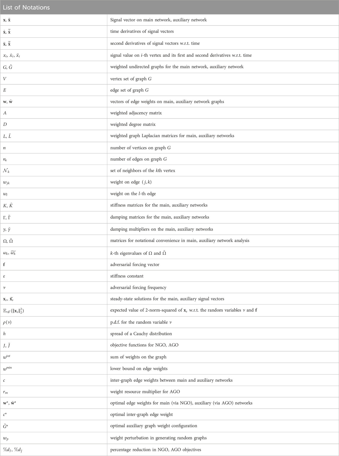
Table 1. List of notations.

The signal on the $k$-th vertex is modeled as a complex number, $x_k\in \mathbb{C}$ (while in practice the signal may be real, in which case the real part of the signal and dynamics equations are of relevance, the equations and their general solutions are compactly represented by a complex dynamics), which follows a second order linear dynamics coupled with the signals on the neighbors of the $k$-th vertex in $G$.

In it is simplest form, such a dynamics can be constructed as a natural extension of the first-order Laplacian dynamics, such that the second derivative of the signal on the $k$-th vertex is equal to the rate of influx of signal from the neighbors of the vertex minus the rate of outflux of signal to the neighbors, with the influx and outflux being proportional to the signal on the respective vertices. With the edge weights identified as the proportionality constants, this simple dynamics can be written as ${\ddot{x}}_k={\sum }_{j\in {\mathcal{N}}_k}{w}_{jk}{x}_j-{\sum }_{j\in {\mathcal{N}}_k}{w}_{jk}{x}_k$.

This dynamics can be compactly written as $\ddot{\mathbf{x}}+L\mathbf{x}=0$, where $\mathbf{x}\in {\mathbb{C}}^n$ is the signal vector (the $k$-th element of which is $x_k$) and $L=D-A$ is the weighted graph Laplacian matrix ($A$ is the weighted adjacency matrix and $D$ the weighted degree matrix).

The Laplacian matrix satisfies the property that its $(j,k)$-th element is zero if there does not exists an edge connecting vertices $k$ and $j$. This property of the Laplacian matrix ensures that the dynamics of signal at a vertex depends on the signals on the neighboring vertices only, and will be referred to as the property of being consistent with the network topology.

In this paper we consider a more general form of second-order linear dynamics for signals following second order differential equation Meirovitch (2010):

$\ddot{\mathbf{x}}+\mathrm{\Gamma }\dot{\mathbf{x}}+K\mathbf{x}=\mathbf{f}{e}^{i\nu t}$

where, $K$ and $\mathrm{\Gamma }$ are the stiffness and damping matrices respectively that are consistent with the network topology (i.e., their $(k,j)$-th element is nonzero only if there exists an edge between the $k$-th and $j$-th vertices in the graph). The network is subject to an adversarial forcing vector $\mathbf{f}$ (with its $k$-th element, $f_k$, being the amplitude of adversarial signal forced on the $k$-th vertex) and forcing frequency $\nu$ (see Figure 1).

Figure 1

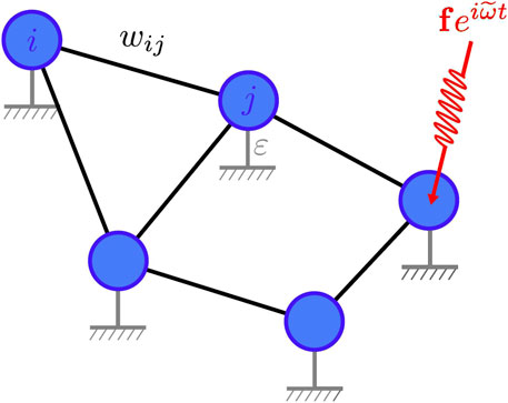
Figure 1. Illustration of a network being attacked by an adversarial agent trying to cause resonance.

The solution to (1), when there is no external forcing (i.e., $\mathbf{f}=\mathbf{0}$), exhibits oscillatory nature when the damping matrix is positive definite and the damping is small Meirovitch (2010). In line with the dynamics of a signal at a vertex being the signed sum of influx and outflux of signals weighed by edge weights, we choose the stiffness matrix to be $K=L+\epsilon I$. The role of the $\epsilon I$ term, for a small $\epsilon >0$, is to ensure that $K$ is positive definite (all eigenvalue of $K$ are strictly greater than zero), which in turn prevents drift in the dynamics, since it is well-known that the weighted graph Laplacian, $L$, has a non-trivial nullspace Godsil et al. (2001). For notational convenience, we also define the matrix $\mathrm{\Omega }$ such that ${\mathrm{\Omega }}^2=K=L+\epsilon I$. We choose the damping matrix as $\mathrm{\Gamma }=2\gamma {\mathrm{\Omega }}^2$ for some small real $\gamma >0$, which corresponds to the fact that the damping over an edge is proportional to the edge weight (scaled by a factor of $2\gamma$). This makes both $K$ and $\mathrm{\Gamma }$ consistent with the network topology. In the later sections, we will assume the damping multiplier $\gamma$ to be small. Using these new notations, we can write the dynamics (1) as $\ddot{\mathbf{x}}+2\gamma {\mathrm{\Omega }}^2\dot{\mathbf{x}}+{\mathrm{\Omega }}^2\mathbf{x}=\mathbf{f}{e}^{i\nu t}$, to which the steady-state solution is given by Meirovitch (2010):

${\mathbf{x}}_s={\left(-{\nu }^{2}I+2i\nu \gamma {\mathrm{\Omega }}^2+{\mathrm{\Omega }}^2\right)}^{-1}\mathbf{f}{e}^{i\nu t}(1)$

It is a well-known fact that if the forcing frequency $\nu$ matches one of the natural frequencies of the network (one of the eigenvalues of $\mathrm{\Omega }$), that leads to resonance, where, with a small damping, the steady-state amplitude of the forced oscillations can get arbitrarily large. The objective of this paper is to minimize the expected steady-state amplitude under a probabilistic model for the distribution of the forcing frequency $\nu$.

We assume that the adversarial agent tries to match its forcing frequency, $\nu$, with one of the natural frequencies of the system (one of the eigenvalues of $\mathrm{\Omega }$), but, is subject to uncertainties, either due to an inability to precisely select the forcing frequency, or because of an imprecise knowledge of the natural frequencies of the system. In particular, we assume that $\nu$ is a stochastic variable with a probability density function dependent upon the natural frequencies of the system.

Definition 1. (Network Vulnerability to Adversarial Resonance Attack). We define the network vulnerability to adversarial resonance attack to be the expected value of the squared 2-norm of the steady-state response, denoted as ${\mathbb{E}}_{\nu ,\mathbf{f}}\left(\Vert {\mathbf{x}}_s{\Vert }_2^2\right)$

The main objective of this work is to develop approaches for optimization of the spectrum of the network graph (i.e., the spectrum of the Laplacian matrix, or equivalently, the spectrum of ${\mathrm{\Omega }}^2$) to reduce the vulnerability of the network against adversarial resonance attacks with a known stochastic model. We approach this problem in two different ways.

(1) A direct optimization of the weights on the edges of the network that minimizes ${\mathbb{E}}_{\nu ,\mathbf{f}}\left(\Vert {\mathbf{x}}_s{\Vert }_2^2\right)$. We refer to this approach as Network Graph Optimization (Section 4).

(2) When it is not possible to alter the weights on the edges directly, we propose to attach an auxiliary network to the main network, and tune/optimize it such that this auxiliary network can effectively absorb and dissipate the excess energy from the resonance in the main network while minimizing the expected steady-state amplitude on the main network. We refer to this approach as Auxiliary Graph Optimization (Section 5).

In this work we only focus on optimizing the weights on the edges of a network graph with fixed topology. However it can be noted that in a weighted graph, a weight of zero on an edge is equivalent to the edge being removed from the graph as far as signal dynamics is concerned. Although it is possible to remove edges with low weight from the graph to sever the signal flow to reduce any potential resonance, this approach would undermine the transmission of the desired signals along the network. We thus use non-zero lower bounds on edge weights when formulating the optimization problems. While addition of edges to the graph is also not addressed within the framework of our optimization problems, starting with a complete graph topology can ensure that all possible edges are present to begin with.

4 Network graph optimization

Given an initial configuration of the main network specified via the graph $G$, the Network Graph Optimization, refers to the procedure of optimizing the main network graph’s weights and/or topology in such a way that the vulnerability of the network is minimized against the adversarial agent’s forcing behavior (forcing vector and frequency) obeying the stochastic model that will be explained in Section 4.1.

In this section, we formulate the spectrum optimization problem to minimize the vulnerability of the network (i.e., the expected value of the squared 2-norm of the steady state response).

4.1 Stochastic model of the adversarial forcing

We assume that the forcing vector $\mathbf{f}$ is sampled from a uniform distribution over a $(n-1)$-unit sphere.

We assume that the adversarial agent has uncertain knowledge of the network (or equivalently precise knowledge of the network, but uncertainty/error in choosing a forcing frequency). This uncertainty/error manifests itself when the adversarial agent tries to pick a forcing frequency that matches one of the natural frequencies of the network. We model this uncertainty by considering $\nu$ to be a random variable whose probability density function, $\rho$, is a uniformly weighted sum of multiple Cauchy distributions Riley et al. (2006), each of which are centered at the natural frequencies, ${\{{\omega }_j\}}_{j=1,\dots ,n}$, with a constant spread of $h$:

$\rho \left(\nu \right)=\frac{1}{n}{\displaystyle \sum _{j=1}^n}{\rho }_{{\omega }_j}\left(\nu \right)=\frac{1}{n}{\displaystyle \sum _{j=1}^n}\frac{h/\pi }{{\left({\omega }_j-\nu \right)}^2+h^2}(2)$

The Cauchy distribution, as opposed to other probability distributions, allows the integral representing the expected value of $\Vert {\mathbf{x}}_s{\Vert }_2^2$ to be efficiently computed. Figure 2 illustrates an example where three individual Cauchy distributions are summed up with uniform weights to obtain a composite probability distribution $\rho (\nu )$.

Figure 2

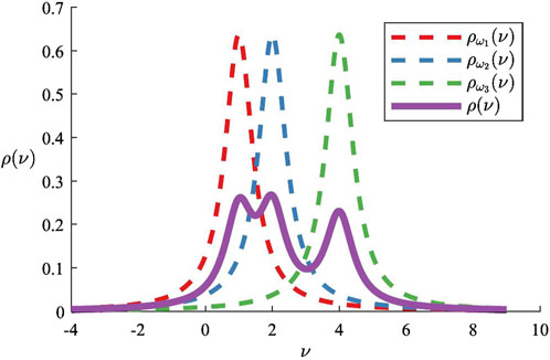
Figure 2. Cauchy distributions centered at the natural frequencies ${\omega }_1=1$, ${\omega }_2=2$, and ${\omega }_3=4$ with a spread of $h=0.5$. The probability density function $\rho (\nu )=\frac{1}{3}{\displaystyle \sum _{i=1}^3}{\rho }_{{\omega }_i}(\nu )$ for the adversarial agent’s choice of forcing frequency is obtained as the uniformly weighted sum of the Cauchy distributions each of which are centered at the natural frequencies of the network.

4.2 Network vulnerability

Following proposition computes the network vulnerability in terms of the spectrum of the network.

Proposition 1. (Network vulnerability). If $\gamma \ll h$, then the network vulnerability is given by ${\mathbb{E}}_{\mathbf{f},\nu }\left(\Vert {\mathbf{x}}_s{\Vert }_2^2\right)=\frac{h}{2\gamma n^2}{\displaystyle \sum _{k,j}}\frac{h^2+{\omega }_k^2+{\omega }_j^2}{{\omega }_k^4\left(h^4+2h^2({\omega }_k^2+{\omega }_j^2)+{({\omega }_k^2-{\omega }_j^2)}^2\right)}$, where ${\omega }_k$ and ${\omega }_j$ are the eigenvalues of $\mathrm{\Omega }$.

In order to prove this result we need the following lemmas.

Lemma 1. If $\mathbf{f}\in {\mathbb{R}}^n$ is sampled from an uniform distribution over a $(n-1)$-unit sphere and $M$ is a symmetric matrix, then ${\mathbb{E}}_{\mathbf{f}}(\Vert M\mathbf{f}{\Vert }_2^2)=\frac{1}{n}\Vert M{\Vert }_F^2$ where $\Vert \cdot {\Vert }_F$ is the Frobenius norm.

The proof of the above lemma is deferred to Appendix 7.1 for better readability.

Lemma 2. If $M_1$ and $M_2$ are real symmetric matrices that commute and $(M_1+i{M}_2)$ is invertible, then $\Vert {(M_1+i{M}_2)}^{-1}{\Vert }_F^2={\sum }_{j=1}^n\frac{1}{{\lambda }_j{(M_1)}^2+{\lambda }_j{(M_2)}^2}$, where ${\lambda }_j(M_1)$ and ${\lambda }_j(M_2)$ denotes the eigenvalues of $M_1$ and $M_2$ corresponding to the $j$-th eigenvector.

The above lemma follows from the definition of the Frobenius norm, $\Vert M{\Vert }_F=\sqrt{Tr(M^{*}M)}$ (where $M^{*}$ denotes the conjugate transpose of $M$).

Proof of Proposition 1. The expected value of $\Vert {\mathbf{x}}_s{\Vert }_2^2$ with respect to the random variables $\mathbf{f}$ and $\nu$ is calculated as follows:

${\mathbb{E}}_{\mathbf{f},\nu }\left(\Vert {\mathbf{x}}_s{\Vert }_2^2\right)=\underset{-\infty }{\overset{\infty }{\int }}{\mathbb{E}}_{\mathbf{f}}\left(\Vert {\mathbf{x}}_s{\Vert }_2^2\right)\rho \left(\nu \right)d\nu (3)$

From Lemma 1 and 2, we have:

${\mathbb{E}}_{\mathbf{f}}\left(\Vert {\mathbf{x}}_s{\Vert }_2^2\right)=\frac{1}{n}\Vert {\left(-{\nu }^{2}I+i2\nu \gamma {\mathrm{\Omega }}^2+{\mathrm{\Omega }}^2\right)}^{-1}{\Vert }_F^2=\frac{1}{n}{\displaystyle \sum _k}\frac{1}{{\left({\omega }_k^2-{\nu }^2\right)}^2+{\left(2\gamma \nu {\omega }_k^2\right)}^2}(4)$

where $(-{\nu }^{2}I+i2\nu \gamma {\mathrm{\Omega }}^2+{\mathrm{\Omega }}^2)$ is always invertible since ${\mathrm{\Omega }}^2=L+\epsilon I$ is positive definite. Substituting Equation 4 into Equation 3, we obtain ${\mathbb{E}}_{\mathbf{f},\nu }\left(\Vert {\mathbf{x}}_s{\Vert }_2^2\right)=\frac{h}{\pi n^2}{\displaystyle \sum _{k,j}}g({\omega }_k^2,{\omega }_j^2)$, where

$g\left({\omega }_k^2,{\omega }_j^2\right)=\underset{-\infty }{\overset{\infty }{\int }}\frac{d\nu }{\left({\left({\omega }_k^2-{\nu }^2\right)}^2+{\left(2\gamma \nu {\omega }_k^2\right)}^2\right)\left({\left({\omega }_j-\nu \right)}^2+h^2\right)}(5)$

Since $\gamma$ is non-zero, the poles of the integrand above lie away from the real line on the complex plane, and hence a closed-form expression for the integral $g({\omega }_k^2,{\omega }_j^2)$ can be obtained using the Residue theorem Saff (2013) by performing a contour integration over the real line and a semi-circular arc of radius $R\to \infty$ on the upper half of the complex plane (Figure 3).

Assuming $\gamma \ll h$, we can compute the roots of the quartic polynomial in $\nu$ in the denominator of the integrand in (6) using a symbolic algebra toolbox, and then apply the Residue theorem to obtain $g({\omega }_k^2,{\omega }_j^2)=\frac{\pi }{2\gamma }\frac{h^2+{\omega }_k^2+{\omega }_j^2}{{\omega }_k^4\left(h^4+2h^2({\omega }_k^2+{\omega }_j^2)+{({\omega }_k^2-{\omega }_j^2)}^2\right)}$. This proves the proposition.

The objective is to minimize this expected value of the 2-norm of the steady-state amplitude, so as to mitigate the effects of resonance attacks on the network. We note that ${\omega }_k$ and ${\omega }_j$ are the eigenvalues of $\mathrm{\Omega }=\sqrt{L+\epsilon I}$, where the Laplacian matrix, $L=D-A$, depends on the weights on the edges of the graph. Thus ${\mathbb{E}}_{\mathbf{f},\nu }\left(\Vert {\mathbf{x}}_s{\Vert }_2^2\right)$, as described in Proposition 1, is a function of the edge weights of the graph. We thus define the objective function, $J(\mathbf{w})={\mathbb{E}}_{\mathbf{f},\nu }\left(\Vert {\mathbf{x}}_s{\Vert }_2^2\right)$ to be a function of the edge weight vector, $\mathbf{w}\in {\mathbb{R}}^m$ (where $m$ is the number of edges in the graph). It can be checked that $J$ is in general a non-convex function. However, if $h$ is large, it can be indeed shown that $J$ is convex in the edge weights.

Figure 3

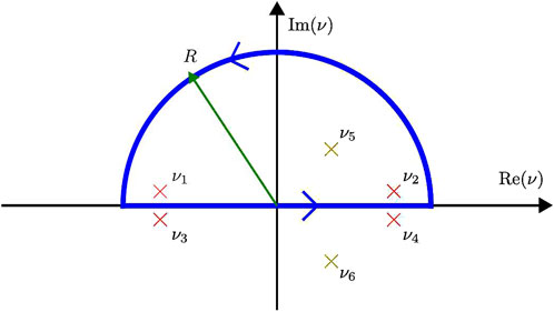
Figure 3. Integration contour for Equation 5. Poles ${\nu }_1$ to ${\nu }_4$ correspond to the forcing vector component ${\mathbb{E}}_{\mathbf{f}}\left(\Vert {\mathbf{x}}_s{\Vert }_2^2\right)$ and they collapse on to the real line as $\gamma$ goes to zero. Poles ${\nu }_5$ and ${\nu }_6$ correspond to the forcing frequency component $\rho (\nu )$.

Proposition 2. For a sufficiently large value of $h$, $J(\mathbf{w})$ is convex.

Proof Sketch. Define the symmetrized function $\tilde{g}({\omega }_k^2,{\omega }_j^2)=\frac{1}{2}\left(g({\omega }_k^2,{\omega }_j^2)+g({\omega }_j^2,{\omega }_k^2)\right)$ so that $J(\mathbf{w})=\frac{h}{\pi n^2}{\sum }_{k,j}\tilde{g}({\omega }_k^2,{\omega }_j^2)$. Since ${\{{\omega }_j^2\}}_{j=\mathrm{1,2},\dots ,n}$ are eigenvalues of ${\mathrm{\Omega }}^2=L+\epsilon I$, we can write $J(\mathbf{w})=\frac{h}{\pi n^2}\mathrm{Tr}(\tilde{g}(L+\epsilon I,L+\epsilon I))$ (where $\tilde{g}(M,N)$ refers to the matrix extension of the scalar function, $\tilde{g}$ Bhattacharya (2025), Bhatia (2013)). It is known that the trace of the matrix extension of a scalar function inherits the convexity properties of the scalar function (see our technical report Bhattacharya (2025) for a detailed proof for the case of multi-variable scalar functions), and as a consequence of that, it is sufficient to show that the function $\tilde{g}$ is convex.

When $h$ is sufficiently large (compared to the eigenvalues of $L$), the function $\tilde{g}$ becomes $\tilde{g}(x,y)=\frac{\pi }{4\gamma }\frac{h^2+x+y}{h^4+2h^2(x+y)+{(x-y)}^2}\left(\frac{1}{x^2}+\frac{1}{y^2}\right)\simeq \frac{\pi }{4\gamma h^2}\left(\frac{1}{x^2}+\frac{1}{y^2}\right)$. It is easy to show that this function is convex in ${\mathbb{R}}_{+}^2$ (a direct computation of the Hessian shows that its eigenvalues are positive). This proves the proposition.

As a consequence of the above proposition, while $J(\mathbf{w})$ may not be strictly convex for all values of $h$, when $h$ is large (corresponding to high uncertainty in the adversarial agent’s ability to choose/apply a forcing that matches a natural frequency of the graph), the objective is indeed convex.

4.3 Spectrum optimization of the main network graph

We define the spectrum optimization problem of the main network graph as the problem of minimizing the expected steady-state amplitude of signal on the network under the described stochastic forcing:

$\begin{array}{cc}\hfill & \underset{\mathbf{w}}{\mathrm{m}\mathrm{i}\mathrm{n}\mathrm{i}\mathrm{m}\mathrm{i}\mathrm{z}\mathrm{e}}J(\mathbf{w})\hfill \\ \hfill & \mathrm{s}\mathrm{u}\mathrm{b}\mathrm{j}\mathrm{e}\mathrm{c}\mathrm{t}\mathrm{t}\mathrm{o}{\mathbf{1}}^T\mathbf{w}=w^{\mathit{tot}},\hfill \\ \hfill & \mathbf{w}⪰w^{\mathit{min}}\mathbf{1}\hfill \end{array}$

where $\mathbf{w}\in {\mathbb{R}}^m$ is the vector of weights on the network graph edges. Here we treat the total sum of weights, ${\sum }_{j=1}^m{w}_j=w^{\mathit{tot}}\ge m{w}^{\mathit{min}}\ge 0$, as a resource to be re-distributed among all edges, hence their sum is constrained to be equal to $w^{\mathit{tot}}$. $w^{\mathit{tot}}$ is assumed to be specified by the initial weight distribution on the network graph $G$.

We consider non-negative edge weights throughout the paper, which further imply $w^{\mathit{min}}>0$ to preserve the connectivity and network topology. Note that $\mathbf{w}$ only contains the weights of the existing edges on the graph, thus it is not possible to remove existing edges or add non-existent edges during the optimization.

The optimal edge weights are denoted by ${\mathbf{w}}^{*}$ and the corresponding optimal weighted graph is $G^{*}=(V,E,{\mathbf{w}}^{*})$. In Figure 4, we provide a histogram of eigenvalues of the graph Laplacian matrix (henceforth referred to as the eigenvalue spectrum) for both the initial network graph $G$ and the optimized network graph $G^{*}$, where both graphs are complete (i.e., there exists an edge between every pair of vertices in $V$). As can be seen, the optimization has the effect of flattening the eigenvalue spectrum, resulting in a more uniform distribution of the eigenvalues, compared to the initial peaky spectrum where the eigenvalues are accumulated around a specific value.

Figure 4

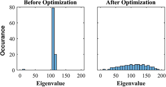
Figure 4. Histograms of the Laplacian matrix eigenvalues for the initial network graph $G$ and optimized network graph $G^{*}$. The initial network is modeled by a complete graph, whose edge weights are perturbed away from a uniform distribution by a small amount. The corresponding spectrum (on the left) is peaky, whereas as a result of the spectrum optimization, the spectrum (on the right) has become flatter.

Observing that the eigenvalues of the graph Laplacian, ${\{{\lambda }_k\}}_{k=\mathrm{1,2},\dots ,n}$, and the eigenvalues of $\mathrm{\Omega }$, ${\{{\omega }_k\}}_{k=\mathrm{1,2},\dots ,n}$, are related monotonically as ${\omega }_k=\sqrt{{\lambda }_k+\epsilon }$, the interpretation of this change in the eigenvalue spectrum is as follows: If a graph has a peaky spectrum, an adversarial agent will have a higher chance of success in causing resonance (high-amplitude oscillations) in the graph by choosing the frequency near the peak to pump its forcing signal into the graph. Whereas, with a flattened spectrum, it has less obvious peak to choose from, and hence the overall expected steady-state amplitude is lower.

In this paper the optimization problem is solved in a centralized manner. A reformulation of $J(\mathbf{w})$ that is amenable to decentralized computation is a significant theoretical endeavor and is outside the scope of this paper.

5 Auxiliary graph optimization

We consider the scenario where the main network cannot be manipulated directly and the edge weights of the main graph $G$ cannot be modified. An alternative to changing the network itself at the level of individual edges of the network is to connect the network with an auxiliary network that is tuned/optimized in a way that minimizes the vulnerability of the main network. This idea of using auxiliary systems to dampen certain frequencies of oscillation appear extensively in the study and design of mechanical and structural systems (such as the use of tuned mass dampers in prevention of mechanical vibrations in buildings Aly (2014)). We, however, develop the mathematical foundations and methods for designing analogous tuned auxiliary networks for mitigating resonance attacks on the network by an adversarial agent.

In this section, we first reformulate the dynamics equations and the definition of vulnerability based on the combined network (main network $+$ auxiliary network). Then, we derive the corresponding objective function and formulate the spectrum optimization problem to minimize the vulnerability of the main network.

5.1 Formulation of combined dynamics

We denote the graph representation of the auxiliary network by $\tilde{G}$, and the combined network is denoted by $G\cup \tilde{G}$ (see Figure 5). A second-order unforced signal dynamics on the stand-alone auxiliary network is given by $\ddot{\stackrel{̃}{\mathbf{x}}}+\tilde{\mathrm{\Gamma }}\dot{\stackrel{̃}{\mathbf{x}}}+\tilde{K}\tilde{\mathbf{x}}=0$, where $\tilde{\mathbf{x}}\in {\mathbb{C}}^{\tilde{n}}$ is the signal vector on the vertices of the auxiliary-network, and $\tilde{\mathrm{\Gamma }}$ and $\tilde{K}$ are the damping and stiffness matrices respectively that are consistent with the topology of the auxiliary network (in particular, $\tilde{K}={\tilde{\mathrm{\Omega }}}^2=\tilde{L}+\epsilon I$ and $\tilde{\mathrm{\Gamma }}=2\tilde{\gamma }{\tilde{\mathrm{\Omega }}}^2$ (where $\tilde{L}$ is the weighted Laplacian matrix of the auxiliary network and $\tilde{\gamma }$ is the damping multiplier on the auxiliary network).

Figure 5

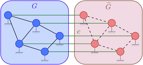
Figure 5. Illustration of an auxiliary graph $\tilde{G}$ attached to the original graph $G$ with an aim to decrease vulnerability against adversarial attacks. The auxiliary graph is of type mirrored (has the same connectivity as the main graph). Green lines indicate the inter-graph connections with weights $c$.

We make the following simplifying assumptions about the auxiliary network and its inter-connection with the main network.

i. We assume the auxiliary network has the same number of vertices as the main network (i.e., $\tilde{n}=n$).

ii. The above assumption allows a one-to-one connection between the vertices of $G$ and $\tilde{G}$. The indexing of the vertices of $\tilde{G}$ is done in a way that the $k$-th vertex of $G$ is assumed to be connected with (and only with) the $k$-th vertex of $\tilde{G}$.

iii. The inter-connecting edges between $G$ and $\tilde{G}$ are assumed to have stiffness (corresponding to a weight of $c$ on those edges), but no damping, allowing the second derivative of the signal on a vertex in $G$ to be coupled with the signal on the neighbor in $\tilde{G}$, but not its first derivative.

iv. It is assumed that the adversarial agent can attack the main network, but not the auxiliary network.

v. The connectivity of the auxiliary graph is specified via one of the two types: (1) a mirrored auxiliary graph, which exactly mirrors the connectivity of the main graph, and (2) a complete auxiliary graph, which is a complete graph. Note that when the main graph is complete, both types correspond to the same auxiliary graph.

Since the auxiliary network is connected to the main network, with the purpose of mitigating the resonance on the main network under adversarial forcing, based on the above assumptions, the signal dynamics over $G$ and $\tilde{G}$ are coupled to give the following signal dynamics on $G\cup \tilde{G}$:

$\left[\begin{array}{c}\hfill \ddot{\mathbf{x}}\hfill \\ \hfill \ddot{\stackrel{̃}{\mathbf{x}}}\hfill \end{array}\right]+\left[\begin{array}{cc}\hfill \mathrm{\Gamma }\hfill & \hfill 0\hfill \\ \hfill 0\hfill & \hfill \tilde{\mathrm{\Gamma }}\hfill \end{array}\right]\left[\begin{array}{c}\hfill \dot{\mathbf{x}}\hfill \\ \hfill \dot{\stackrel{̃}{\mathbf{x}}}\hfill \end{array}\right]+\left[\begin{array}{cc}\hfill K+cI\hfill & \hfill -cI\hfill \\ \hfill -cI\hfill & \hfill \tilde{K}+cI\hfill \end{array}\right]\left[\begin{array}{c}\hfill \mathbf{x}\hfill \\ \hfill \tilde{\mathbf{x}}\hfill \end{array}\right]=\left[\begin{array}{c}\hfill \mathbf{f}\hfill \\ \hfill 0\hfill \end{array}\right]e^{i\nu t}$

where the terms $cI$ represent coupling between the dynamics of the two networks due to the one-to-one connection between the vertices of $G$ and $\tilde{G}$, and affects the stiffness matrix of the combined network, but not the damping matrix. An illustration of a combined network is provided in Figure 5.

5.2 Network vulnerability with attached auxiliary network

Following proposition gives the vulnerability of a network to which we attach the auxiliary network.

Proposition 3. (Network vulnerability with attached auxiliary network). The vulnerability of a network to which an auxiliary network is attached is given by

${\mathbb{E}}_{\mathbf{f},\nu }\left(\Vert {\mathbf{x}}_s{\Vert }_2^2\right)=\frac{1}{n^2}{\displaystyle \sum _j}{\int }_{\infty }^{\infty }{‖{\left(\left(i\nu 2\gamma {\mathrm{\Omega }}^2+{\mathrm{\Omega }}^2+\left(c-{\nu }^2\right)I\right)+c^2{\left(i\nu 2\tilde{\gamma }{\tilde{\mathrm{\Omega }}}^2+{\tilde{\mathrm{\Omega }}}^2+\left(c-{\nu }^2\right)I\right)}^{-1}\right)}^{-1}‖}_F^2{\rho }_{{\omega }_j}\left(\nu \right)d\nu$

where ${\rho }_{{\omega }_j}(\nu )=\frac{h/\pi }{{({\omega }_j-\nu )}^2+h^2}$.

When $\mathrm{\Omega }$ and $\tilde{\mathrm{\Omega }}$ are simultaneously diagonalizable, this can be further simplified to

${\mathbb{E}}_{\mathbf{f},\nu }\left(\Vert {\mathbf{x}}_s{\Vert }_2^2\right)=\frac{1}{n^2}{\displaystyle \sum _{k,j}}\underset{-\infty }{\overset{\infty }{\int }}{s}_k\left(\nu \right){\bar{s}}_k\left(\nu \right){\rho }_{{\omega }_j}\left(\nu \right)d\nu$

where $s_k(\nu )=\frac{1}{-{\nu }^2+i\nu 2\gamma {\omega }_k^2+{\omega }_k^2+c-\frac{c^2}{-{\nu }^2+i\nu 2\tilde{\gamma }{\tilde{\omega }}_k^2+{\tilde{\omega }}_k^2+c}}$ with ${\tilde{\omega }}_k$ denoting the $k$-th eigenvalue of $\tilde{\mathrm{\Omega }}$ and ${\bar{s}}_k$ denoting the complex conjugate of $s_k$.

Note that in either of the expressions for ${\mathbb{E}}_{\mathbf{f},\nu }\left(\Vert {\mathbf{x}}_s{\Vert }_2^2\right)$ above, the network vulnerability is expressed as a function of the weights on the edges of the main and auxiliary networks–first one in terms of Frobenius norm of a matrix involving $\mathrm{\Omega }$ and $\tilde{\mathrm{\Omega }}$, and the second one more explicitly in terms of their eigenvalues.

Proof. The steady-state solution to (8) is

$\left[\begin{array}{c}\hfill {\mathbf{x}}_s\hfill \\ \hfill {\tilde{\mathbf{x}}}_s\hfill \end{array}\right]=S^{-1}\left[\begin{array}{c}\hfill \mathbf{f}\hfill \\ \hfill 0\hfill \end{array}\right]e^{i\nu t}\text{,\hspace{0.17em}where,}(6)$

$S=\left[\begin{array}{cc}\hfill i\nu 2\gamma {\mathrm{\Omega }}^2+{\mathrm{\Omega }}^2+\left(c-{\nu }^2\right)I\hfill & \hfill -cI\hfill \\ \hfill -cI\hfill & \hfill i\nu 2\tilde{\gamma }{\tilde{\mathrm{\Omega }}}^2+{\tilde{\mathrm{\Omega }}}^2+\left(c-{\nu }^2\right)I\hfill \end{array}\right](7)$

However, we note that we are only interested in the response of the main network to the adversarial attacks, which from (Equations 6, 7) is:

${\mathbf{x}}_s={\left[S^{-1}\right]}_{11}\mathbf{f}{e}^{i\nu t}(8)$

where ${[S^{-1}]}_{11}$ is the top left $n\times n$ block of the inverse of the matrix $S$, which can be computed using Schur complement of a block matrix Boyd and Vandenberghe (2004) as:

$\begin{array}{cc}\hfill {\left[S^{-1}\right]}_{11}& ={\left({\left[S\right]}_{11}-{\left[S\right]}_{12}{\left[S\right]}_{22}^{-1}{\left[S\right]}_{21}\right)}^{-1}\hfill \\ \hfill & ={\left(\left(i\nu 2\gamma {\mathrm{\Omega }}^2+{\mathrm{\Omega }}^2+\left(c-{\nu }^2\right)I\right)+c^2{\left(i\nu 2\tilde{\gamma }{\tilde{\mathrm{\Omega }}}^2+{\tilde{\mathrm{\Omega }}}^2+\left(c-{\nu }^2\right)I\right)}^{-1}\right)}^{-1}\hfill \end{array}(9)$

(As a quick sanity check, note that when $c=0$, which means that the main and the auxiliary networks are not connected, we have

${\left[S^{-1}\right]}_{11}={\left(i\nu 2\gamma {\mathrm{\Omega }}^2+{\mathrm{\Omega }}^2-{\nu }^{2}I\right)}^{-1}(10)$

indicating that the steady-state response on the main network is equivalent to the one derived in Equation 1, as expected. In Section 6 we use this theoretical result to perform further numerical sanity check on the Auxiliary Graph Optimization objective function.)

If $\mathrm{\Omega }$ and $\tilde{\mathrm{\Omega }}$ are simultaneously diagonalizable, using (Equation 9), allows us to compute the eigenvalues of ${[S^{-1}]}_{11}$ as:

$s_k\left(\nu \right)=\frac{1}{-{\nu }^2+i\nu 2\gamma {\omega }_k^2+{\omega }_k^2+c-\frac{c^2}{-{\nu }^2+i\nu 2\tilde{\gamma }{\tilde{\omega }}_k^2+{\tilde{\omega }}_k^2+c}}(11)$

According to the stochastic model explained in Section 4.1, $\mathbf{f}$ is being uniformly sampled from $(n-1)$-unit sphere and the adversarial agent only has imprecise information about the main graph (i.e., it has no information about the auxiliary graph and hence the combined network) leading to the probability density function (3) for the forcing frequency $\nu$.

Rest of the proof is similar to the proof of Proposition 1. We use Lemma 1 and Lemma 2, and Equation 11 to compute the expected value with respect to $\mathbf{f}$ the result of the proposition then follows from the substitution of this expected value together with the p. d.f. (Equation 2) into Equation 3.

Later on, we will show that there will be an approximation error between the computed expected value and the average squared 2-norm of the steady-state response when $\mathrm{\Omega }$ and $\tilde{\mathrm{\Omega }}$ are not simultaneously diagonalizable.

A closed form expression for the integral in Proposition 3 is obtained using the Residue theorem with the same contour as before as described in Section 4.2. In order to use the Residue theorem as described, however, one needs to compute the roots of the quartic polynomial in $\nu$ in the denominator of the integrand and determine whether those roots have positive or negative imaginary parts. In this case a direct computation of that, even using a symbolic algebra toolbox, was not feasible because of the complexity of the problem. In order to simplify computation of the roots, we use linearization with respect to $\gamma$. The details of the computation are provided in Appendix 7.2. Corresponding calculations are performed using a symbolic mathematics toolbox. We omit the resulting expression for brevity.

Assuming that the main graph $G$ and the parameters $n$, $h$, $\gamma$ remain constant, the objective is to minimize ${\mathbb{E}}_{\mathbf{f},\nu }\left(\Vert {\mathbf{x}}_s{\Vert }_2^2\right)$, which is a function of the eigenvalues of the auxiliary stiffness matrix $\tilde{\mathrm{\Omega }}$ (which, in turn, are functions of the weights on the auxiliary graph edges, $\tilde{\mathbf{w}}$), the uniform inter-graph edge weight $c$ and the auxiliary damping factor $\tilde{\gamma }$. For the purposes of this paper, we assume $\tilde{\gamma }$ to be a small constant, in order to allow signals transmitted over the network (non-adversarial) to persist and not get dissipated too quickly. The resulting objective function is thus defined as $\tilde{J}(\tilde{\mathbf{w}},c)={\mathbb{E}}_{\mathbf{f},\nu }\left(\Vert {\mathbf{x}}_s{\Vert }_2^2\right)$.

5.3 Spectrum optimization of the auxiliary network graph

We define the spectrum optimization problem of the auxiliary network graph as follows:

$\begin{array}{cc}\hfill & \underset{\tilde{\mathbf{w}},c}{\mathrm{m}\mathrm{i}\mathrm{n}\mathrm{i}\mathrm{m}\mathrm{i}\mathrm{z}\mathrm{e}}\tilde{J}(\tilde{\mathbf{w}},c)\hfill \\ \hfill & \mathrm{s}\mathrm{u}\mathrm{b}\mathrm{j}\mathrm{e}\mathrm{c}\mathrm{t}\mathrm{t}\mathrm{o}\mathbf{0}⪯\tilde{\mathbf{w}},\hfill \\ \hfill & 0\le c,\hfill \\ \hfill & {\mathbf{1}}^T\tilde{\mathbf{w}}+nc\le r_m{w}^{\mathit{tot}}\hfill \end{array}$

Here, we assume that the weight resource is specified as a multiple of the total weights on the main graph (denoted by $r_m{w}^{\mathit{tot}}$) which is to be distributed among the auxiliary graph and inter-graph edges. We consider non-negative edge weights throughout, without any additional lower bound.

The optimal auxiliary graph edge weights are denoted by ${\tilde{\mathbf{w}}}^{*}$, the optimal inter-graph edge weight is $c^{*}$ and the corresponding optimal auxiliary graph weight configuration is ${\tilde{G}}^{*}$.

Note that it is also possible to consider the case where the auxiliary damping multiplier $\tilde{\gamma }$ is a decision variable. We include further discussion on the effects of the auxiliary damping and experimental results in Section 6.3.4.

6 Results

In this section, we present experiments conducted to accomplish the following.

• Validate the accuracy of the objective functions, $J$ and $\tilde{J}$, in representing the network vulnerability measured by $\mathbb{E}(\Vert {\mathbf{x}}_s{\Vert }_2^2)$ for ${\mathbf{x}}_s$ defined on $G$ and $\tilde{G}$, as described in Proposition 1 and 3 respectively.

• Analyze the effects of the problem parameters associated with the network dynamics and constraints on the relative vulnerability decrease that can be achieved via the proposed methods.

• Demonstrate the effectiveness of the proposed methods in decreasing the network vulnerability across a variety of problem instances.

• Perform numerical simulation of dynamics over a network to further validate the results achieved by the Network Graph Optimization.

• Apply the network graph optimization to the communication network among a team of mobile robots between which the signal strength decays with increasing distance.

6.1 Implementation details and setup

We solve the network graph and auxiliary graph spectrum optimizations using the interior-point algorithm The MathWorks (2023).

6.1.1 Network graph construction

All algorithms are implemented and tested on three classes of network graphs.

i. Random Complete Graphs (“RCG”): Given the number of vertices, $n$, we establish an edge between every pair of vertices, thus resulting in a graph with $n_e=\dim \mathbf{w}=\left(\genfrac{}{}{0ex}{}{n}{2}\right)$edges. We then sample the weight for each edge from an uniform distribution on the interval $[1-w_p,1+w_p]$, where $w_p$ is a given weight perturbation.

ii Random Incomplete Graphs (“RIG”): Given the number of vertices, $n$, and the number of edges, $n_e=\dim \mathbf{w}<\left(\genfrac{}{}{0ex}{}{n}{2}\right)$, we randomly chose $n_e$ distinct pair of vertices to establish the edges between. Weights for the edges are sampled from an uniform distribution on the interval $[1-w_p,1+w_p]$.

iii. Social Network Graphs (“Social”): As a representative of real-world networks, we extracted subgraphs from the “Government” graph category of the Gemsec Facebook Dataset Rozemberczki et al. (2019) which encompasses various graphs representing blue verified Facebook page networks. To generate the subgraphs, ego graphs with a radius of two were created. Nodes were randomly selected without replacement to serve as the center of each ego graph. Only the first 100 subgraphs containing between 25 and 200 vertices that were generated were selected, resulting in a set of 100 subgraphs with an average 109.82 vertices and 867.69 edges per subgraph.

6.1.2 Adversarial force sampling

For computing steady-state amplitudes for specific instances of simulation for a given graph, we need to sample the adversarial forcing vector, $\mathbf{f}$, and the adversarial forcing frequency, $\nu$.

As described in Section 4.1, we assume that the forcing vector $\mathbf{f}$ is sampled from an $(n-1)$-dimensional unit sphere. This is achieved by sampling each element of the vector from the standard normal distribution, and then normalizing the vector Muller (1959). Here we highlight that the necessary number of forcing vector samples to cover the sphere surface increases exponentially as the size of the network, $n$, (the dimension of the forcing vector/unit sphere) increases, if the sample dispersion is to be maintained. This comes from the fact that the dispersion is inversely proportional to the sample size and the dimension Sukharev (1971); Deheuvels (1983).

As described in Section 4.1, the forcing frequency needs to be sampled using a probability density function that is a uniformly weighted sum of multiple Cauchy distributions each of which are centered at the natural frequencies, ${\{{\omega }_j\}}_{j=1,\dots ,n}$, with a constant spread of $h$. However, in order to perform this sampling, one needs to compute the inverse of the cumulative distribution function (c.d.f.) of the $\rho$ described in Equation 2, which is computationally difficult. We thus adopt a practical method that is used to generate samples from mixture models as explained in Moitra (2018): Using an uniform probability of $1/n$ on all the natural frequencies, ${\{{\omega }_j\}}_{j=1,\dots ,n}$, we first sample one of the natural frequencies, say ${\omega }_s$. Then the forcing frequency is sampled from a Cauchy distribution centred at ${\omega }_s$ and with a spread of $h$ using the inverse c. d.f. of Cauchy distribution, $\nu ={\omega }_s+h\tan \left(\pi (p-0.5)\right.$, where $p$ is sampled from an uniform distribution over the unit interval [0,1].

6.2 Network graph optimization

First we present the results from Network Graph Optimization.

6.2.1 Validation of the objective function

The objective function, $J$ (Proposition 1), for the network graph spectrum optimization problem is the expected value of the squared 2-norm of the steady-state response of the dynamic network subject to adversarial forcing with the stochastic model explained in Section 4.1.

To validate the accuracy of the objective function in representing the expected value, we generate 400M adversarial forcing samples (using the procedure explained in Section 6.1), evaluate the closed-form steady state response, ${\mathbf{x}}_s$, for each sample using Equation 1 and compute the average squared 2-norm of the responses $\overline{\Vert {\mathbf{x}}_s{\Vert }_2^2}$. For the validation study, we use a RCG with $n=10$ and $w_p=0.3$. The running average over the number of samples divided in multiple batches are provided in Figure 6.

Figure 6

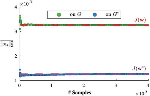
Figure 6. Squared 2-norm of the steady state response ${\mathbf{x}}_s$ is evaluated in closed-form using sampled external forcing. This plot shows the running average of $\Vert {\mathbf{x}}_s{\Vert }_2^2$ against the number of forcing samples. The running averages are computed using batches of 100K samples. Over large enough samples, the average $\overline{\Vert {\mathbf{x}}_s{\Vert }_2^2}$ evaluated on the initial graph $G$ and the optimized graph $G^{*}$ converge to the values of the objective function evaluated at $\mathbf{w}$ and ${\mathbf{w}}^{*}$ respectively.

It can be observed that over a large number of forcing samples, the average of the squared 2-norm of the steady-state responses is well approximated by the objective values for both initial and optimized graphs. Hence, ${\mathbb{E}}_{\mathbf{f},\nu }\left(\Vert {\mathbf{x}}_s{\Vert }_2^2\right)$ is accurately represented by $J$. Consequently, it can be seen that on the optimized graph, the steady state responses have smaller amplitudes on average. Following this validation, we can use the objective value as a measure of a graph’s vulnerability to adversarial attacks, where a lower objective function indicates less vulnerability.

6.2.2 Parameter analysis

Each spectrum optimization problem on a network graph can be specified via a set of parameters regarding the second order dynamics of the network, the external forcing and the constraints. These parameters are the number of vertices on the graph $(n)$, the number of edges on the graph $(n_e)$, the minimum weight constraint $(w^{\mathit{min}})$, the stiffness constant $(\epsilon )$, the damping factor $(\gamma )$, and the spread of the external agent’s frequency distribution $(h)$.

We analyze the effects of these parameters on the percentage reduction of objective value that can be achieved via the spectrum optimization, hence the reduction in the vulnerability of the main network graph using the Network Graph Optimization method. For this purpose, we start with set of parameter values, $n=30$, $n_e=225$, $w^{\mathit{min}}=10^{-3}$, $\epsilon =10$, $\gamma =10^{-6}$, $h=0.1$, and generate problem instances featuring both RCGs and RIGs where we vary one parameter and keep the rest constant. We solve for each problem instance and compute the percentage reductions in objective as $\%d_J=\frac{|J^0-J^{*}|}{J^0}\times 100$ (where superscripts 0 and $\ast$ denote initial and optimal objective values), which are plotted against the varying parameter values in Figure 7. Note that by comparing the percentage decrease in the objectives instead of the final objective values achieved, we are trying to isolate the effect of the parameters on the effectiveness of Network Graph Optimization method in reducing the vulnerability of a graph instead of trying to find the set of problem parameters that make the network the least vulnerable.

Figure 7

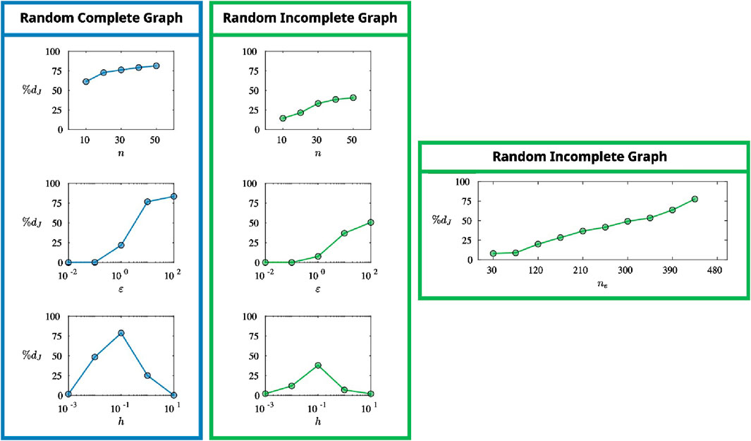
Figure 7. A RCG and a RIG are generated for the problem instances specified by each set of parameters (only a RIG is generated for the case where the variable parameter is the number of edges). The optimization problem is solved for each instance, and the percentage decrease in objective values are plotted against the varying parameter.

It can be observed from Figure 7 that a larger decrease in the objective value can be achieved as the number of vertices or the number of edges increase. Intuitively, more vertices and more edges correspond to more flexibility in distributing the weight resources, thus resulting in larger improvements to the vulnerability of the graph. As expected, larger stiffness yields better results, where the effect gets more significant with increased orders of magnitude. The spread of the external agent’s frequency distribution has a non-monotonic effect. As the spread gets smaller, the agent is able to pick the resonance frequencies more accurately, leaving the graph helpless against the attack, whereas a larger frequency spread corresponds to an agent that almost arbitrarily picks its frequencies, against which any modification of the graph based on reasoning would be less effective. Since the minimum weight constraint and the damping factor did not demonstrate a significant effect on the percentage decrease of the objective, corresponding plots are excluded. By observing the plots overall and the analysis on the number of edges, it is clear that the spectrum optimization on a main network graph is more effective when the graph is complete. This behavior will become more apparent in the next section.

6.2.3 Demonstration of the effectiveness of network graph optimization

To demonstrate the overall effectiveness of spectrum optimization on the main network graph in reducing the network vulnerability, we solve the optimization problem for RCGs, RIGs and Social graphs, and show that significant decrease in objective values can be achieved. We generate 100 RCGs and RIGs with $n$ sampled uniformly from the interval [10, 30] and $w_p$ sampled uniformly from the interval [0.1,0.5]. For the RIGs, we sampled $n_e$ from the interval $[n,n^2/4]$. While in a real-world problem, the parameters would be provided based on the properties of the network and the adversarial agent, for the purpose of demonstration of the effectiveness of the Network Graph Optimization, based on the parameter analysis in the previous section we choose a set of values for which the effects our approach are more apparent. The parameters associated with the network dynamics are the minimum weight, $w^{\mathit{min}}=0.001$, the stiffness constant, $\epsilon =10$, the damping coefficient, $\gamma =10^{-6}$, and the adversarial agent’s frequency spread, $h=0.1$. The average percentage decrease in the objective value and the standard deviation across the problem instances featuring RCGs, RIGs and Social graphs are provided in Figure 8. Qualitatively, on the spectrum of the graph, the optimization is manifested as a flattening of the spectrum, as can be seen for the complete graph in Figure 9A and the Social graph in Figure 9B.

Figure 8

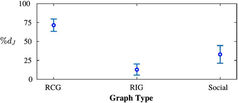
Figure 8. The network graph spectrum optimization problem is solved for instances featuring 100 RCGs, 100 RIGs and 100 social network graphs. On problems instances where the main network graphs are complete, the optimization consistently yielded larger relative decrease in the objective values.

Figure 9

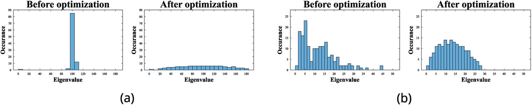
Figure 9. Left (a): Example of eigenvalue spectrum of a complete graph before and after optimization represented as histograms of the eigenvalues of the networks stiffness matrix, $L+\epsilon I$. The objective value significantly decreased from 1.378 to 0.3778, yielding a 72.58% decrease as a result of the network graph optimization on a 100-node RCG. Qualitatively, as a result of the network graph optimization, the eigenvalue spectrum has become flatter. Right (b): Example of eigenvalue spectrum of a representative Facebook Social subgraph before and after optimization represented as histograms of the eigenvalues of the networks stiffness matrix, $L+\epsilon I$. The objective value significantly decreased from 6.868 to 2.467 as a result of the network graph optimization on the 173-node Facebook social subgraph, corresponding to a 64.089% decrease in the objective value. As a result of the optimization, the eigenvalue spectrum has become smoother and flatter.

As mentioned before, network graph spectrum optimization is more successful at reducing the objective value relative to the initial value of the objective when it is performed on complete graphs. A reason for this behavior is the greater vulnerability of the complete graphs to the resonance attacks, due to the fact that the natural frequencies of a complete graph are heavily accumulated around a value resulting in a peaky spectrum, compared to a relatively flatter/uniform distribution of the natural frequencies on an incomplete graph. A fewer number of optimization variables impose greater rigidity on incomplete graphs due to their fewer edges, whereas complete graphs, with their maximum possible number of edges, offer a greater flexibility in edge weight manipulations. Qualitatively, this is manifested by a lower relative flattening of the spectrum in case of the incomplete Social graph (Figure 9B) as compared to the complete graph (Figure 9A).

6.2.4 Numerical second-order dynamics simulation of the main network

We considered an unoptimized complete graph with uniform edge weights with an added perturbation as detailed in Section 6.1, as well as the corresponding optimized graph obtained using the network graph optimization method detailed in Section 4, and performed 100 numerical simulations (via numerical integration) of the second-order dynamics on each of these graphs with varying forcing vectors and sampled forcing frequencies. The simulations were run until a steady state was achieved. The squared amplitude of $\mathbf{x}$ as a function of time for each of the 100 simulations, each normalized by the closed-form steady-state squared amplitude $\Vert {\mathbf{x}}_s{\Vert }^2$, is shown in Figure 10. Besides observing that the steady-state amplitudes of the numerical simulations match the computed closed-form values, we note that the unsteady amplitude in relation to the steady-state amplitude has less variation in the optimized graph.

Figure 10

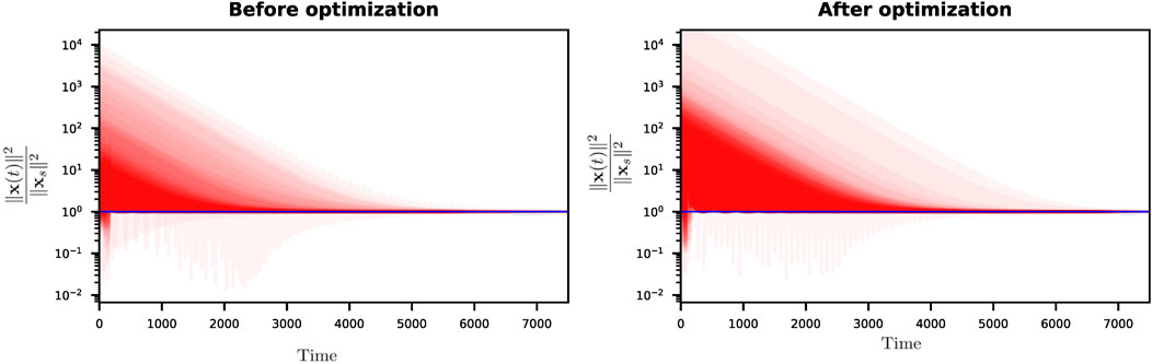
Figure 10. Normalized amplitude plot of 100 different numerical simulations of the second-order dynamics for both the initial and optimized complete graph, displaying their corresponding two-norm squared amplitude values divided by the steady-state squared amplitude value calculated by the closed-form evaluation for the respective forcing vector and forcing frequency (i.e., $\frac{\Vert \mathbf{x}(t){\Vert }^2}{\Vert {\mathbf{x}}_s{\Vert }^2}$). Since the two-norm squared amplitude value from the simulation of the second-order dynamics should converge to the same closed-form steady-state evaluation for the two-norm squared amplitude given the same corresponding forcing vector and forcing frequency, the values in the plot are expected to approach 1, as indicated by the blue line, which they indeed do. In these 100 simulations, the initial graph’s mean steady-state squared amplitude value is 0.0899, while the optimized graph’s mean steady-state squared amplitude value is 0.0145.

6.2.5 Network Vulnerability Reduction in a Mobile Robot Network

We consider a team of $n$ mobile robots and their communication network desc-ribed by a complete graph. The signal strength between robot $i$ and $j$ (represented by the edge weight $w_{ij}$) is computed as: $w_{ij}=\frac{A_{\mathit{dist}}}{\Vert r_i-r_j\Vert +{\epsilon }_{\mathit{dist}}}$, where $A_{\mathit{dist}}$ and ${\epsilon }_{\mathit{dist}}$ are constant parameters, and $r_i$ refers to the positions the $i$-th robot.

Considering the weights to be functions of robot positions, $J(\mathbf{w}(\mathbf{r}))$, we solve the optimization problem defined in Section 4.3 with respect to the robot positions, with an additional constraint, $\Vert r_i-r_j\Vert \ge d_{\mathit{min}}$, on the separation between the robots in order to prevent robot collisions.

We consider three types of initial configurations for the robots: arbitrary placement within some bounding box, on a uniform grid, on a line. We generate 10 instances for each initial condition where some small random perturbation is applied to the robot locations. Following parameters are used for the experiments: $n=30$, $w^{\mathit{min}}=0.001$, $\epsilon =1$, $\gamma =10^{-6}$, $h=0.1$, $A_{\mathit{dist}}=1$, ${\epsilon }_{\mathit{dist}}=0.1$, $d_{\mathit{min}}=1$.

The mean and the standard deviation of the objective reduction achieved from each type of initial configuration is reported in the table in Figure 11. The initial and optimal robot locations for a problem instance with 64 robots is provided in Figure 11. Our observation suggests that optimization of the network vulnarability results in a reorganization of the robots in an approximate multi-layer formation.

Figure 11

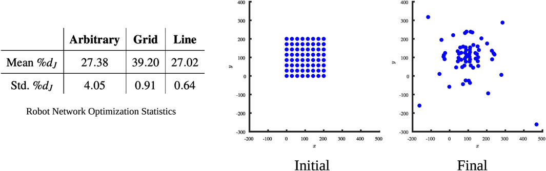
Figure 11. Vulnerability reduction in a mobile robot network. Left: Mean and the standard deviation of the objective reduction achieved. Right: an example initial and final (after network vulnerability minimization) arrangement of a group of 64 robots.

6.3 Auxiliary graph optimization

For the Auxiliary Graph Optimization approach, we conduct similar experiments and provide additional analysis on the effects of auxiliary damping.

6.3.1 Validation of the objective function

The objective function $\tilde{J}$ for the auxiliary graph spectrum optimization problem is the expected value of the squared 2-norm of the steady-state response corresponding to the main network vertices when the dynamic network is subject to stochastic adversarial forcing.

To validate the accuracy of the objective function in representing the expected value, we generate 800M adversarial forcing samples, evaluate the closed-form steady state responses for each sample using Equation 8 and compute the average squared 2-norm of the responses. For the validation study, we generate a RCG with $n=10$, with $w_p=0.3$ and use it as the main network graph. The running average over the number of samples divided in multiple batches are provided in Figure 12A.

Figure 12

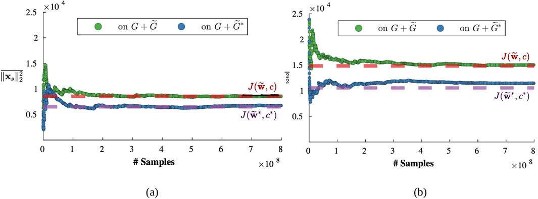
Figure 12. Squared 2-norm of the steady state response corresponding to the main graph ${\mathbf{x}}_s$ is evaluated in closed-form using sampled external forcing. This plot shows the running average of $\Vert {\mathbf{x}}_s{\Vert }_2^2$ against the number of forcing samples. The running averages are computed using batches of 100K samples. Left (a): Over large enough samples, the average $\overline{\Vert {\mathbf{x}}_s{\Vert }_2^2}$ evaluated on the unoptimized combined network system $G+\tilde{G}$ and the optimized system $G+{\tilde{G}}^{*}$ converge to the values of the objective function evaluated at $(\tilde{\mathbf{w}},c)$ and $({\tilde{\mathbf{w}}}^{*},c^{*})$ respectively. Right (b): Over large enough samples, the average $\overline{\Vert {\mathbf{x}}_s{\Vert }_2^2}$ evaluated on the unoptimized combined network system $G+\tilde{G}$ converges to the values of the objective function evaluated at $(\tilde{\mathbf{w}},c)$. However, when evaluated on the optimized system $G+{\tilde{G}}^{*}$ the average $\overline{\Vert {\mathbf{x}}_s{\Vert }_2^2}$ does not converge to the value of the objective function evaluated at $({\tilde{\mathbf{w}}}^{*},c^{*})$, resulting in an approximation error.

The problem instance generated for the validation study resulted in an optimized auxiliary graph for which $\mathrm{\Omega }$ and ${\tilde{\mathrm{\Omega }}}^{*}$ are simultaneously diagonalizable. As a consequence, we observe that $\overline{\Vert {\mathbf{x}}_s{\Vert }_2^2}$ converge to the objective values for both the optimized and unoptimized combined networks. To demonstrate the fact that there will be an approximation error between $\overline{\Vert {\mathbf{x}}_s{\Vert }_2^2}$ and $\tilde{J}$, when $\mathrm{\Omega }$ and ${\tilde{\mathrm{\Omega }}}^{*}$ are not simultaneously diagonalizable, we perform another auxiliary graph spectrum optimization based on a RIG with $n=10$, $n_e=25$ and $w_p=0.3$. The running average over the number of samples divided in multiple batches are provided in Figure 12B.

From Figures 12A, B, it can be observed that over a large number of forcing samples, the average of the squared 2-norm of the steady-state responses is well approximated by the objective values when $\mathrm{\Omega }$ and $\tilde{\mathrm{\Omega }}$ are simultaneously diagonalizable, whereas there exist an approximation error when these matrices are not simultaneously diagonalizable. Also, it can be seen that on the optimized graphs, the steady state responses have smaller amplitudes on average.

As a sanity check, we leverage the theoretical result provided in Equation 10 and confirm that $J$ and $\tilde{J}$ match when evaluated numerically for arbitrary choices of $\mathrm{\Omega }$ and $\tilde{\mathrm{\Omega }}$ when $c=0$.

Following the validation of the objective function $\tilde{J}$, we can use the objective value as a measure of a graph’s vulnerability to adversarial attacks, where a lower objective function indicates less vulnerability.

6.3.2 Parameter analysis

Parameters that specify an spectrum optimization problem on an auxiliary graph is similar to those of network graph optimization. Since the auxiliary graph edges and inter-graph edges are assumed to have non-negative weights, we do not consider the minimum weight constraint $(w^{\mathit{min}})$ parameter in this case. However, in addition to the network graph optimization parameters, we must consider the effects of the following parameters associated with auxiliary graphs: the auxiliary connectivity type (mirrored or complete), the weights resource multiplier $r_m$, and the auxiliary damping factor $\tilde{\gamma }$. We defer the analysis of the auxiliary damping factor to Section 6.3.4 and use a constant auxiliary damping factor of $\tilde{\gamma }=10^{-6}$ throughout the parameter analysis.

We analyze the effects of these parameters on the percentage reduction of objective value that can be achieved via the auxiliary graph optimization, hence the relative decrease in the vulnerability of the graph using the Auxiliary Graph Optimization method. We start with the same set of parameter values with the addition of $r_m=5$, and generate problem instances where we vary one parameter and keep the rest constant. We solve for each problem instance and compute the percentage reductions in objective as $\%d_{\tilde{J}}=\frac{|J^0-{\tilde{J}}^{*}|}{J^0}\times 100$, which are plotted against the varying parameter values in Figure 13. Note that for the problem instances where the main network graph is a RIG, we provide two sets of results achieved with a mirrored auxiliary graph and a complete auxiliary graph.

Figure 13

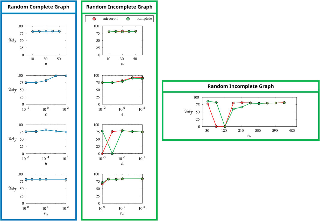
Figure 13. A RCG and a RIG is generated for the problems specified by each set of parameters (only a RIG is generated for variable $n_e$). The optimization problem is solved for each instance (using both mirrored and complete auxiliary graphs for instances where the network graph is incomplete), and the percentage decrease in objective values $(\%d_{\tilde{J}})$ are plotted against the varying parameter. Data points where the percentage decrease is at 0 indicate the instances where the optimization failed to converge within the maximum number of iterations.

Here we highlight that the percentage reduction of the objective value is computed based on the value of the objective before the auxiliary graph is attached, that is $J^0$, instead of the objective value evaluated using an unoptimized auxiliary graph, that is ${\tilde{J}}^0=\tilde{J}(\tilde{\mathbf{w}},c)$. The individual effects of attaching an arbitrary auxiliary graph, and the optimization of the auxiliary graph will be presented in the next section.

For all parameters, effects are similar to those on the network graph optimization. However, even for the parameter values for which the network graph optimization was less effective, the Auxiliary Graph Optimization method can achieve larger decreases in the objective, which makes the approach less sensitive to the choice of the parameters. The same insensitivity is observed to the weight resource multiplier parameter. For the instances where the network graph was incomplete, some of the optimizations of the mirrored auxiliary graph failed to converge in the maximum number of iterations considered, which is indicated by a $0\%$ decrease in the plots.

6.3.3 Demonstration of the effectiveness of auxiliary graph optimization

To demonstrate the overall effectiveness of spectrum optimization on the auxiliary graph in reducing the network vulnerability, we solve the optimization problem for RCGs and RIGs and show that significant decrease in objective values can be achieved. We use the same problem instances generated for the network graph optimization, with $r_m=5$ and $\tilde{\gamma }=10^{-6}$ and using complete auxiliary graphs. To demonstrate the effects of attaching an arbitrary auxiliary graph and the optimization of this auxiliary graph separately, we provide the average and the standard deviation of the percentage decrease in the objective calculated as (1) $\%d_{\tilde{J}}=\frac{|J^0-{\tilde{J}}^0|}{J^0}\times 100$ (decrease achieved by going from network configuration $G$ to $G+\tilde{G}$), and (2) $\%d_{\tilde{J}}=\frac{|J^0-{\tilde{J}}^{*}|}{J^0}\times 100$ (decrease achieved by going from network configuration $G$ to $G+{\tilde{G}}^{*}$) across the problem instances featuring complete and incomplete main network graphs are provided in Figure 14.

Figure 14

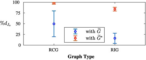
Figure 14. The auxiliary graph spectrum optimization problem is solved for instances featuring 100 RCGs and 100 RIGs. We report the average and standard deviation of the percentage decrease in the objective achieved by both going from the network configuration $G$ to $G+\tilde{G}$ and from the network configuration $G$ to $G+{\tilde{G}}^{*}$. Success rates for running Auxiliary Graph Optimization on RCGs and RIGs were $\%100$ and $\%97$ respectively.

It can be seen that attaching even an arbitrary auxiliary graph decreases the vulnerability of the network significantly. However, performing the optimization over the auxiliary edge weights and inter-graph edges results in a further decrease of the vulnerability and provides more consistent behavior.

6.3.4 Effect of the auxiliary damping and auxiliary damping optimization

Assuming that the auxiliary graph weights and the inter-graph edge weights are constant, the auxiliary objective function $\tilde{J}$ becomes a function of the auxiliary damping factor $\tilde{\gamma }$ only. Furthermore, if the auxiliary damping is uniform across all auxiliary vertices, $\tilde{J}$ is a single-variable function. To visualize the effect of the auxiliary damping, we evaluate $\tilde{J}$ on an optimized combined network (specified by $G,{\tilde{G}}^{*},c^{*}$) with $\tilde{\gamma }$ varying logarithmically on the interval $[10^{-6},10^5]$. The objective values are plotted against the auxiliary damping factor in Figure 15.

Figure 15

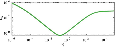
Figure 15. Value of the auxiliary objective function $\tilde{J}$ evaluated on an optimized combined network (specified by $G,{\tilde{G}}^{*},c^{*}$) with auxiliary damping factor $\tilde{\gamma }$ on the interval $[10^{-6},10^5]$.

We observe that the objective function $\tilde{J}$ is highly sensitive to the value of the auxiliary damping $\tilde{\gamma }$ and that one can significantly decrease the objective value by setting the auxiliary damping to be larger than the damping on the main network. However, simply setting the auxiliary damping to the maximum allowed value does not yield the smallest objective value as observed from Figure 15. To the best of our understanding, as the auxiliary damping gets larger than the optimal value, the auxiliary network loses the ability to dissipate the signal that is being transmitted from the main network and the signal tends to bounce back causing a resonance. For this reason, optimizing over the variable $\tilde{\gamma }$ could provide further improvements if the goal is to achieve the least possible vulnerability in the network.

7 Conclusion and discussions

In this paper, we developed the notion of vulnerability of a network with second order signal dynamics under adversarial forcing that obeys a known stochastic model. To minimize the network vulnerability, we proposed two methods that optimize the network structure: i. The Network Graph Optimization method provides an optimal set of network edge weights under the condition that the edge weights can be directly manipulated, and, ii. The Auxiliary Graph Optimization method allows us to design an auxiliary network that can be attached to the main network with the purpose of minimizing the vulnerability, when the main network edge weights cannot be adjusted directly. We conducted numerical experiments to analyze the two methods in detail.

Currently, the notion of vulnerability and the optimization problems posed in this work depend on a linear model of the signal dynamics and a specific stochastic model of adversarial forcing. While the adaptation of some aspects of the model to other setting (e.g., a different stochastic model of adversarial forcing) can be straight-forward re-derivation of the objective functions, a more general formulation that encompasses more complicated signal models, forcing models, and potentially nonlinear signal dynamics, is within the scope of future work. The optimization formulations presented in this paper lead to generally non-convex problems which are in turn solved by gradient based solvers. While we do show convexity (Proposition 2) of the objective function of the Network Graph Optimization problem under the assumption that the parameter $h$ is large, a more general analysis of the optimization landscape for finite values of $h$ would be necessary to provide guarantees on the quality of the solution being returned, both for the Network Graph Optimization as well as the Auxiliary Graph Optimization problems. Such analyses are within the scope of future work.

The current optimization problem is formulated as a centralized one that assumes complete knowledge of the network graph edge weights. This limits the scalability of the optimization problem to larger networks. A potential future work involves the development of a distributed optimization scheme in which each vertex would use information about its local subgraph and would only adjusts weights on its incident edges in order to optimize the network. A distributed method would allow the approach to scale to larger networks and generalize to settings where global information regarding the network may not be available due to privacy restrictions. In future we will work towards implementing the proposed methods on real-world, physical networks such as electrical grids, robot networks and social networks.

Data availability statement

The original contributions presented in the study are included in the article/supplementary material, further inquiries can be directed to the corresponding author.

Author contributions

AS: Data curation, Software, Visualization, Writing – original draft, Writing – review and editing, Formal Analysis, Validation. NK: Data curation, Software, Writing – original draft, Writing – review and editing. RB: Conceptualization, Investigation, Supervision, Writing – original draft, Writing – review and editing. SB: Conceptualization, Formal Analysis, Investigation, Methodology, Project administration, Software, Supervision, Writing – original draft, Writing – review and editing.

Funding

The author(s) declare that financial support was received for the research and/or publication of this article. This work was supported by AFOSR award number FA9550-23-1-0046.

Acknowledgments

We gratefully acknowledge the support of AFOSR award number FA9550-23-1-0046. We would like to thank Brian M. Sadler, Senior Research Fellow, University of Texas at Austin, for his valuable insights and discussions on the motivation and potential applications of this work during the course of writing this paper.

Conflict of interest

The authors declare that the research was conducted in the absence of any commercial or financial relationships that could be construed as a potential conflict of interest.

Generative AI statement

The author(s) declare that no Generative AI was used in the creation of this manuscript.

Publisher’s note

All claims expressed in this article are solely those of the authors and do not necessarily represent those of their affiliated organizations, or those of the publisher, the editors and the reviewers. Any product that may be evaluated in this article, or claim that may be made by its manufacturer, is not guaranteed or endorsed by the publisher.

References

Aly, A. M. (2014). Proposed robust tuned mass damper for response mitigation in buildings exposed to multidirectional wind. Struct. Des. Tall Special Build. 23, 664–691. doi:10.1002/tal.1068

CrossRef Full Text | Google Scholar

Bhatia, R. (2013). Matrix analysis, 169. Springer Science and Business Media.

Google Scholar

Bhattacharya, S. (2025). Trace of multi-variable matrix functions and its application to function of graph spectrum. arXiv e-prints. arXiv:2501.14515. doi:10.48550/arXiv.2501.14515

CrossRef Full Text | Google Scholar

Boyd, S., and Vandenberghe, L. (2004). Convex optimization. Cambridge University Press.

Google Scholar

Chan, H., and Akoglu, L. (2016). Optimizing network robustness by edge rewiring: a general framework. Data Min. Knowl. Discov. 30, 1395–1425. doi:10.1007/s10618-015-0447-5

CrossRef Full Text | Google Scholar

Chen, Y., Ye, H., Vedula, S., Bronstein, A., Dreslinski, R., Mudge, T., et al. (2023). Demystifying graph sparsification algorithms in graph properties preservation. Proc. VLDB Endow. 17, 427–440. doi:10.14778/3632093.3632106

CrossRef Full Text | Google Scholar

Cheng, X., Kawano, Y., and Scherpen, J. M. A. (2017). Reduction of second-order network systems with structure preservation. IEEE Trans. Automatic Control 62, 5026–5038. doi:10.1109/TAC.2017.2679479

CrossRef Full Text | Google Scholar

Chow, J., and Kokotovic, P. (1985). Time scale modeling of sparse dynamic networks. IEEE Trans. Automatic Control 30, 714–722. doi:10.1109/TAC.1985.1104055

CrossRef Full Text | Google Scholar

De Gennaro, M. C., and Jadbabaie, A. (2006). “Decentralized control of connectivity for multi-agent systems,” in Proceedings of the 45th IEEE conference on decision and control, 3628–3633. doi:10.1109/CDC.2006.377041

CrossRef Full Text | Google Scholar

Deheuvels, P. (1983). Strong bounds for multidimensional spacings. Z. für Wahrscheinlichkeitstheorie Verwandte Geb. 64, 411–424. doi:10.1007/BF00534948

CrossRef Full Text | Google Scholar

Dorfler, F., Simpson-Porco, J. W., and Bullo, F. (2018). Electrical networks and algebraic graph theory: models, properties, and applications. Proc. IEEE 106, 977–1005. doi:10.1109/JPROC.2018.2821924

CrossRef Full Text | Google Scholar

Freitas, S., Yang, D., Kumar, S., Tong, H., and Chau, D. H. (2022). Graph vulnerability and robustness: a survey. IEEE Trans. Knowl. Data Eng. 35, 1–5934. doi:10.1109/TKDE.2022.3163672

CrossRef Full Text | Google Scholar

Godsil, C., Royle, C., and Royle, G. (2001). “Algebraic graph theory,” in Graduate texts in mathematics (Springer).

Google Scholar

Griparic, K., Polic, M., Krizmancic, M., and Bogdan, S. (2022). Consensus-based distributed connectivity control in multi-agent systems. IEEE Trans. Netw. Sci. Eng. 9, 1264–1281. doi:10.1109/TNSE.2021.3139045

CrossRef Full Text | Google Scholar

Hashemi, M., Gong, S., Ni, J., Fan, W., Prakash, B. A., and Jin, W. (2024). A comprehensive survey on graph reduction: sparsification, coarsening, and condensation. Proc. Thirty-ThirdInternational Jt. Conf. Artif. Intell., 8058–8066. doi:10.24963/ijcai.2024/891

CrossRef Full Text | Google Scholar

Meirovitch, L. (2010). Fundamentals of vibrations. Waveland Press.

Google Scholar

Mirzaev, I., and Gunawardena, J. (2013). Laplacian dynamics on general graphs. Bull. Math. Biol. 75, 2118–2149. doi:10.1007/s11538-013-9884-8

PubMed Abstract | CrossRef Full Text | Google Scholar

Moitra, A. (2018). Gaussian mixture models. Cambridge University Press.

Google Scholar

Mox, D., Kumar, V., and Ribeiro, A. (2022). Learning connectivity-maximizing network configurations. IEEE Robotics Automation Lett. 7, 5552–5559. doi:10.1109/LRA.2022.3146524

CrossRef Full Text | Google Scholar

Muller, M. E. (1959). A note on a method for generating points uniformly on n-dimensional spheres. Commun. ACM 2, 19–20. doi:10.1145/377939.377946

CrossRef Full Text | Google Scholar

Nagpal, S. V., Nair, G. G., Parise, F., and Anderson, C. L. (2023). Designing robust networks of coupled phase oscillators with applications to the high voltage electric grid. IEEE Trans. Control Netw. Syst. 10, 1046–1057. doi:10.1109/tcns.2022.3214778

CrossRef Full Text | Google Scholar

Olfati-Saber, R. (2006). Flocking for multi-agent dynamic systems: algorithms and theory. IEEE Trans. Automatic Control 51, 401–420. doi:10.1109/TAC.2005.864190

CrossRef Full Text | Google Scholar

Olfati-Saber, R., and Murray, R. (2004). Consensus problems in networks of agents with switching topology and time-delays. IEEE Trans. Automatic Control 49, 1520–1533. doi:10.1109/TAC.2004.834113

CrossRef Full Text | Google Scholar

Pan, L., Shao, H., and Mesbahi, M. (2016). “Laplacian dynamics on signed networks,” in 2016 IEEE 55th conference on decision and control (CDC), 891–896. doi:10.1109/CDC.2016.7798380

CrossRef Full Text | Google Scholar

Ren, W., Beard, R., and Atkins, E. (2005). A survey of consensus problems in multi-agent coordination. Proc. 2005, Am. Control Conf. 2005, 1859–1864. doi:10.1109/ACC.2005.1470239

CrossRef Full Text | Google Scholar

Riley, K. F., Hobson, M. P., and Bence, S. J. (2006). Mathematical methods for physics and engineering: a comprehensive guide. Cambridge University Press.

Google Scholar

Romeres, D., Dã¶rfler, F., and Bullo, F. (2013). “Novel results on slow coherency in consensus and power networks,” in 2013 European control conference (ECC), 742–747. doi:10.23919/ECC.2013.6669400

CrossRef Full Text | Google Scholar

Rozemberczki, B., Davies, R., Sarkar, R., and Sutton, C. (2019). “Gemsec: graph embedding with self clustering,” in Proceedings of the 2019 IEEE/ACM international Conference on Advances in social networks Analysis and mining 2019 (ACM), 65–72.

Google Scholar

Saff, E. B. (2013). Fundamentals of complex analysis with applications to engineering. Pearson.

Google Scholar

Saif, M., Javad-Kalbasi, M., and Valaee, S. (2024). Effectiveness of reconfigurable intelligent surfaces to enhance connectivity in uav networks. IEEE Trans. Wirel. Commun. 23, 18757–18773. doi:10.1109/TWC.2024.3476422

CrossRef Full Text | Google Scholar

Sheng, L., Lou, G., Gu, W., Lu, S., Ding, S., and Ye, Z. (2022). Optimal communication network design of microgrids considering cyber-attacks and time-delays. IEEE Trans. Smart Grid 13, 3774–3785. doi:10.1109/TSG.2022.3169343

CrossRef Full Text | Google Scholar

Spielman, D. A., and Srivastava, N. (2008). “Graph sparsification by effective resistances,” in Proceedings of the fortieth annual ACM symposium on theory of computing (New York, NY, USA: Association for Computing Machinery), STOC ’08), 563â€, 568. doi:10.1145/1374376.1374456

CrossRef Full Text | Google Scholar

Sukharev, A. (1971). Optimal strategies of the search for an extremum. USSR Comput. Math. Math. Phys. 11, 119–137. doi:10.1016/0041-5553(71)90008-5

CrossRef Full Text | Google Scholar

Sun, C., Dai, R., and Mesbahi, M. (2018). Weighted network design with cardinality constraints via alternating direction method of multipliers. IEEE Trans. Control Netw. Syst. 5, 2073–2084. doi:10.1109/tcns.2018.2789726

CrossRef Full Text | Google Scholar

The MathWorks (2023). Optimization toolbox user’s guide. r2023b edn. Natick, MA, USA: The MathWorks, Inc.

Google Scholar

van der Schaft, A. J., and Maschke, B. M. (2013). Port-Hamiltonian systems on graphs. SIAM J. Control Optim. 51, 906–937. doi:10.1137/110840091

CrossRef Full Text | Google Scholar

Zhang, L., Sadler, B. M., Blum, R. S., and Bhattacharya, S. (2021). Inter-cluster transmission control using graph modal barriers. IEEE Trans. Signal Inf. Process. over Netw. 7, 275–293. doi:10.1109/TSIPN.2021.3071219

CrossRef Full Text | Google Scholar

Appendix

7.1 Proof of lemma one

Statement of the Lemma If $\mathbf{f}\in {\mathbb{R}}^n$ is sampled from an uniform distribution over a $(n-1)$-unit sphere and $M$ is a symmetric matrix, then

${\mathbb{E}}_{\mathbf{f}}\left(\Vert M\mathbf{f}{\Vert }_2^2\right)=\frac{1}{n}\Vert M{\Vert }_F^2$

where $\Vert \cdot {\Vert }_F$ is the Frobenius norm.

Proof. Suppose $M$ is diagonalized by the orthogonal matrix $U$, so that $M=UD{U}^T$, where $D=\mathrm{d}\mathrm{i}\mathrm{a}\mathrm{g}(d_1,d_2,\dots ,d_n)$ is the diagonal matrix of the eigenvalues of $M$.

Because of rotational symmetry of the distribution of $\mathbf{f}$ (uniform distribution over a sphere), the expected value of $\Vert M\mathbf{f}{\Vert }_2^2$ is independent of the choice of (an orthonormal) basis, and in particular, is the same in the basis of the eigenvectors of $M$. Thus,

${\mathbb{E}}_{\mathbf{f}}\left(\Vert M\mathbf{f}{\Vert }_2^2\right)={\mathbb{E}}_{\mathbf{f}}\left(\Vert D\mathbf{f}{\Vert }_2^2\right)={\mathbb{E}}_{\mathbf{f}}\left({\displaystyle \sum _{j=1}^n}{d}_j^2{f}_j^2\right)={\displaystyle \sum _{j=1}^n}{d}_j^2\mathbb{E}\left(f_j^2\right)(12)$

where $\mathbb{E}(f_j^2)$ is the expected value of the square of the $j$-th component of $\mathbf{f}$.

However, we note that because of the spherical symmetry of the distribution of $\mathbf{f}$, we must have $\mathbb{E}(f_1^2)=\mathbb{E}(f_2^2)=\cdots =\mathbb{E}(f_n^2)≕\xi$. Thus,

$\begin{array}{ll}\hfill & {\mathbb{E}}_{\mathbf{f}}\left(\Vert \mathbf{f}{\Vert }_2^2\right)=1={\displaystyle \sum _{j=1}^n}\mathbb{E}\left(f_j^2\right)=n\xi \hfill \\ \hfill & \Rightarrow \xi =1/n\hfill \end{array}$

Hence from (Equation 12) we have, ${\mathbb{E}}_{\mathbf{f}}(\Vert M\mathbf{f}{\Vert }_2^2)={\sum }_{j=1}^n{d}_j^2/n=\frac{1}{n}\Vert M{\Vert }_F^2$.

7.2 Approximate root computation using linearization

Consider a polynomial in the variable $x\in \mathbb{C}$, given by $Q(x,\gamma )$, where $\gamma \in \mathbb{R}$ is a parameter involved in the coefficients of the polynomial. We are interested in approximately computing the roots of the polynomial for a general small, positive parameter value, $\gamma$, given the roots of the polynomial when $\gamma =0$ (which is presumed to be easier to compute).

If ${\{r_k(\gamma )\}}_{k=\mathrm{1,2},\dots ,n}$ are the roots of the polynomial $Q(x,\gamma )$ (possibly with multiplicity), we have

$\begin{array}{ll}\hfill & Q\left(x,\gamma \right)=\prod _{k=1}^n\left(x-r_k\left(\gamma \right)\right)\hfill \\ \hfill & \Rightarrow \frac{\partial Q}{\partial \gamma }\left(x,\gamma \right)=-{\displaystyle \sum _{l=1}^n}{r}_l^{\prime }\left(\gamma \right)\prod _{k\ne l}\left(x-r_k\left(\gamma \right)\right)\hfill \end{array}$

Evaluating the above at $x=r_j(\gamma )$,

$\begin{array}{ll}\hfill & \frac{\partial Q}{\partial \gamma }\left(r_j\left(\gamma \right),\gamma \right)=-r_j^{\prime }\left(\gamma \right)\prod _{k\ne j}\left(r_j\left(\gamma \right)-r_k\left(\gamma \right)\right)\hfill \\ \hfill & \Rightarrow r_j^{\prime }\left(\gamma \right)=-\frac{\frac{\partial Q}{\partial \gamma }\left(r_j\left(\gamma \right),\gamma \right)}{{\prod }_{k\ne j}\left(r_j\left(\gamma \right)-r_k\left(\gamma \right)\right)}\hfill \end{array}$

This gives first order approximations for $r_j(\gamma )$ in the neighborhood of $\gamma =0$

$\begin{array}{ll}\hfill r_j\left(\gamma \right)& \approx r_j\left(0\right)+r_j^{\prime }\left(0\right)\gamma \hfill \\ \hfill & =r_j\left(0\right)-\frac{\frac{\partial Q}{\partial \gamma }\left(r_j\left(0\right),0\right)}{{\prod }_{k\ne j}\left(r_j\left(0\right)-r_k\left(0\right)\right)}\gamma \hfill \end{array}$