Planar Formation Control of a School of Robotic Fish: Theory and Experiments

This paper presents a nonlinear control design for the stabilization of parallel and circular motion in a school of robotic fish actuated with internal reaction wheels. The closed-loop swimming dynamics of the fish robots are represented by the canonical Chaplygin sleigh. They exchange relative state information according to a connected, undirected communication graph to form a system of coupled, nonlinear, second-order oscillators. Prior work on collective motion of constant-speed, self-propelled particles serves as the foundation of our approach. However, unlike a self-propelled particle, the fish robots follow limit-cycle dynamics to sustain periodic flapping for forward motion with time-varying speed. Parallel and circular motions are achieved in an average sense without feedback linearization of the agents’ dynamics. Implementation of the proposed parallel formation control law on an actual school of soft robotic fish is described, including system identification experiments to identify motor dynamics and the design of a motor torque-tracking controller to follow the formation torque control. Experimental results demonstrate a school of four robotic fish achieving parallel formations starting from random initial conditions.

1 Introduction

Collective behavior of mobile agents has received significant interest recently in fields such as biology, physics, computer science, and control engineering (Reynolds, 1987; Vicsek et al., 1995; Ren et al., 2007). Research in this area is allowing scientists to better understand swarming behavior in nature and benefits control engineers in numerous applications by mimicking nature’s behavior in engineered mobile systems such as unmanned ground, air, and underwater vehicles.

Previous investigations of bioinspired underwater vehicles include the design, sensing, and control of a single fish-inspired robot that is driven by an internal reaction wheel (Zhang et al., 2016; Free et al., 2017; Lee et al., 2019). Here, we present control laws that stabilize planar formations of a school of such robotic fish (Figure 1). Related work involving formation experiments of fish robots propelled by tail flapping was presented in (Berlinger et al., 2021; Zhang et al., 2021). In (Berlinger et al., 2021), a school of fish robots achieves circular formations and other collective behaviors using vision-based behaviors based on relative position. Similarily, in (Zhang et al., 2021), parallel and circular formations are achieved using an overhead camera to provide absolute positions of all the agents. Our work differs in that we investigate synchronized motion of multiple fish robots driven by an internal reaction wheel. We utilize consensus control to achieve collective motion by communicating only relative position and/or orientation with nearby agents. This approach is particularly well suited to challenging underwater environments where small, low-power robots have limited communication or sensing range.

FIGURE 1

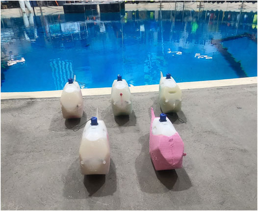
FIGURE 1. A school of soft robotic fish serves as a testbed for formation control experiments at the University of Maryland’s Neutral Buoyancy Research Facility.

Consensus control in Euclidean space, which assumes that the states of the system live on ${\mathbb{R}}^N$, is a well-studied topic (Cao et al., 2013). The goal of consensus control is to steer N agents into identical states. Similarly, average-consensus control laws steer agents towards the average value of the initial conditions of the agents (Olshevsky, 2015). Consensus and average consensus are typically studied for single-integrator dynamics (Ren and Beard, 2005), which may contain linear or nonlinear drift vector fields (Cao and Ren, 2012). Interactions between agents can be static (Chopra, 2012), time-varying (Moreau, 2005), all-to-all (Chopra, 2012), or limited (Li et al., 2011). These interactions are typically described using the Laplacian matrix from algebraic graph theory (Horn and Johnson, 1990) to compute relative state information, such as relative position. Consensus and average consensus in Euclidean space have also been studied for double-integrator dynamics (Zhang and Tian, 2009) and second-order systems with a nonlinear drift vector field that represents the vehicle dynamics (Yu et al., 2010). Furthermore, consensus control on a nonlinear manifold has been investigated (Scardovi et al., 2007; Paley, 2009). For example, consensus on the N-torus—also called synchronization—arises in the control of planar formations, where the heading orientation is a phase angle on the unit circle (Sepulchre et al., 2007). Orientation and translation control of agents in the plane utilizes the special Euclidean group (Justh and Krishnaprasad, 2004). Many synchronization approaches are based on the theory of coupled oscillators, such as the celebrated Kuramoto model (Sepulchre et al., 2007), and invoke the graph Laplacian for cooperative control of first-order dynamics on the N-torus (Sepulchre et al., 2008). Second-order consensus of coupled oscillators with double-integrator dynamics (Napora and Paley, 2013) uses the gradient of a phase potential.

Another class of collective behaviors of multi-agent systems are circular formations. Previous work in this area studied circular formations of first-order, self-propelled particles with unit velocity. Feedback control laws designed in (Sepulchre et al., 2007) stabilize a circular formation having a fixed center and a constant radius. Some extensions to this work consider a circular formation in a flow field (Paley, 2008) and constant non-unitary velocity, or with a constraint bounding the circular formation to a region of interest (Jain and Ghose, 2019). Other extensions include time-varying centers, so that the circular formation position is not fixed (Brinón-Arranz et al., 2014; Yu and Liu, 2017). Some authors assume agents use relative-position sensing to achieve circular formations around a given center and radius that is known only to a subset of agents (Yu et al., 2018). Circular formation control on the tangent bundle of the N-torus has also been investigated where agents are second-order self-propelled particles (Sepulchre et al., 2007; Napora and Paley, 2013).

This work investigates planar formations in a novel setting: a system of second-order oscillators with nonlinear dynamics and nonholonomic constraints on the tangent bundle of the N-torus. The closed-loop swimming dynamics of the fish robots are represented by the Chaplygin sleigh (Kelly et al., 2012), (Lee et al., 2019), a nonholonomic mechanical system driven by an internal reaction wheel. Our control design is inspired by prior work on collective motion of self-propelled particles (Paley, 2007; Sepulchre et al., 2007; Paley, 2008; Napora and Paley, 2013); however, a key distinction is that agents have second-order limit-cycle dynamics with time-varying speed. Thus, novel parallel and circular formations are achieved in an average sense.

The contributions of this paper are 1) a control design that achieves parallel motion for a school of robotic fish, represented by a system of coupled, nonlinear, second-order oscillators with Chaplygin sleigh dynamics using only relative state information; 2) a control design that achieves circular motion for the same system; 3) system identification of the reaction-wheel motor dynamics and the design of an optimal estimation and tracking controller that follows the torque commands of the formation control; and 4) experimental validation of the parallel formation control law on a school of bio-inspired robotic fish (Figure 1). The proposed control algorithms are illustrated through both numerical simulations and experiments in the University of Maryland’s Neutral Buoyancy Research Facility.

The remainder of the paper is organized as follows. Section 2 provides preliminaries on graph theory, the self-propelled particle model, and Chaplygin sleigh dynamics. Section 3 present control designs to achieve parallel and circular formations for a robotic fish school. Section 4 presents the experimental implementation and results for the parallel formation control for a school of robotic fish. Lastly, Section 5 summarizes the paper and discusses ongoing and future work.

2 Background

This section reviews concepts from graph theory, presents the self-propelled particle model, and summarizes the dynamics of a Chaplygin sleigh, used to model our robotic fish.

2.1 Graph Theory

A graph is used to represent the communication topology of an interacting system of agents. The communication graph is built upon a set of nodes $\mathcal{V}=\{1,\dots ,N\}$ that represent agents. An edge denoted by the pair (k, j) exists between agent $k\in \mathcal{V}$ and $j\in \mathcal{V}$ if information flows from j to k. The set of all edges is denoted $\mathcal{E}\subseteq {\mathcal{V}}^2$. The set of nodes $\mathcal{V}$ and the edges $\mathcal{E}$ define a graph $G=(\mathcal{V},\mathcal{E})$ (Diestel, 2000). A sequence of edges {(k, k₁), (k₁, k₂), …, (k_ξ, j)} with distinct nodes $k_l\in \mathcal{V}$, k_l ≠ k, k_l ≠ j, for l = 1, 2, …, ξ is called a path from node k to node j. A graph G is called undirected if $(k,j)\in \mathcal{E}$ implies $(j,k)\in \mathcal{E}$. For a undirected graph, the set of neighbors to node k is denoted ${\mathcal{N}}_k=\{v\in \mathcal{V}:(k,v)\in \mathcal{E}\}$. If there exists a path between any pair of distinct nodes $k,j\in \mathcal{V}$, then an undirected graph G is called connected. Edges are expressed using the adjacency matrix $A\in {\mathbb{R}}^{N\times N}$, where the entry on the kth row and jth column is

$A_{kj}=\left\{\begin{array}{cc}1\hfill & \text{if}\left(k,j\right)\in \mathcal{E}\hfill \\ 0\hfill & \text{otherwise}.\hfill \end{array}\right.$

The degree matrix $D\in {\mathbb{R}}^{N\times N}$ encodes how many unique edges are connected to each node and has nonzero elements on the diagonal, i.e.,

$D_{kj}=\left\{\begin{array}{cc}{\sum }_{n=1}^N{A}_{kn}\hfill & \text{if}k=j\hfill \\ 0\hfill & \text{otherwise}.\hfill \end{array}\right.$

The symmetric and positive semi-definite Laplacian matrix $L\in {\mathbb{R}}^{N\times N}$ associated with the undirected graph G is L = D − A. The Laplacian is used to compute relative state information communicated between agents. The quadratic form z^TLz ≥ 0, where $\mathit{z}\in {\mathbb{R}}^N$, is equal to zero if and only if z_k = z_j, for all $k,j\in \mathcal{V}$.

2.2 Self-Propelled Particle Model

The self-propelled particle model (Justh and Krishnaprasad, 2004) has often been used to describe the collective motion of N planar vehicles that move at a constant speed with steering controls inputs. The planar position of the kth particle with respect to the origin of the inertial frame is expressed using complex coordinates as $r_k=x_k+i{y}_k\in \mathbb{C}$, where $k\in \mathcal{V}$. The dynamics of the kth particle are

$\begin{array}{cc}\hfill {\dot{r}}_k& =v_k{e}^{i{\theta }_k}\hfill \\ \hfill {\dot{\theta }}_k& =u_k,\hfill \end{array}(1)$

where, for the kth particle, $v_k\triangleq \sqrt{{\dot{x}}_k^2+{\dot{y}}_k^2}\in \mathbb{R}$ is a constant speed, ${\theta }_k\triangleq \mathrm{a}\mathrm{t}\mathrm{a}\mathrm{n}({\dot{y}}_k/{\dot{x}}_k)\in \mathbb{T}$ is the orientation of the velocity (also called the phase of the particle), $\mathbb{T}\triangleq \mathbb{S}$ is the torus, and $u_k\in \mathbb{R}$ is the steering control. The unit vector $e^{i{\theta }_k}$ is called the phasor of particle k and is aligned with its heading, whereas $i{e}^{i{\theta }_k}$ is perpendicular to the heading (Figure 2A). For a constant speed, v_k = v₀, and a constant turn-rate, ${\dot{\theta }}_k={\omega }_0$, the particle moves on a circle with radius $|v_0{\omega }_0^{-1}|$ and center $c_k=r_k+i{v}_0{\omega }_0^{-1}{e}^{i{\theta }_k}$. This fixed-radius circle will later serve as a reference for stabilizing circular formations.

FIGURE 2

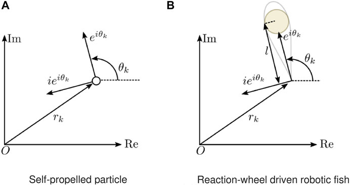
FIGURE 2. Coordinates and unit vectors: (A) the self-propelled particle; (B) the Chaplygin-sleigh model of a robotic fish. In (B), the hydrofoil shape represents the fish robot body and a bronze-colored reaction wheel is shown at the center of mass.

When referring to the positions, phase arrangement, reference circle centers, and control inputs of the collective of N particles, we use bold letters, i.e., $\mathit{r}\triangleq {[r_1,\dots ,r_k]}^{\mathrm{T}}\in {\mathbb{C}}^N$, $\mathit{\theta }\triangleq {[{\theta }_1,\dots ,{\theta }_k]}^{\mathrm{T}}\in {\mathbb{T}}^N$, $\mathit{c}\triangleq {[c_1,\dots ,c_k]}^{\mathrm{T}}\in {\mathbb{C}}^N$, and $\mathit{u}={[u_1,\dots ,u_k]}^{\mathrm{T}}\in {\mathbb{R}}^N$, respectively. Similarly, $e^{i\mathit{\theta }}\triangleq {[e^{i{\theta }_1},\dots ,e^{i{\theta }_k}]}^{\mathrm{T}}\in {\mathbb{C}}^N$. For complex numbers, $z_1,z_2\in \mathbb{C}$, the inner product is defined as $⟨z_1,z_2⟩=\mathrm{R}\mathrm{e}\{\overline{z_1}{z}_2\}$, where $\overline{z_1}$ is the complex conjugate of z₁. This inner product is equivalent to the standard inner product on ${\mathbb{R}}^2$. For complex vectors, $\mathit{z},\mathit{y}\in {\mathbb{C}}^N$, the inner product is similarly defined as $⟨\mathit{z},\mathit{y}⟩={\sum }_{i=1}^N\mathrm{R}\mathrm{e}\{\overline{z_i}{y}_i\}$. The modulus of a complex number is denoted $|\cdot |=\sqrt{⟨\cdot ,\cdot ⟩}$.

Cooperative control laws for stabilizing the collective motion of identical, unit-speed, self-propelled particles in parallel or circular formations have been extended to include an external flow field (Paley, 2008), motion on spherical surfaces (Paley, 2009), and various communication topologies (Sepulchre et al., 2007; Sepulchre et al., 2008). For parallel formations, all particles are synchronized when they have equal and constant phase, θ = θ₀1, where 1 = [1,…,1]^T is the N-by-1 vector of ones, for some constant ${\theta }_0\in \mathbb{T}$. For synchronization, the relative positions of particles are arbitrary. For circular formations, all particles move in the same direction along the same circle, that is, $\dot{\theta }={\omega }_0\mathit{1}$ for some constant ω₀ and c = c₀1 for some constant $c_0\in \mathbb{C}$. In a circular formation, the relative phases of the particles are arbitrary.

Parallel and circular formations may be achieved using Lyapunov-based control design to minimize a potential function for a desired formation. Consider the Laplacian parallel formation potential (Paley, 2007)

$U_p\left(\mathit{\theta }\right)\triangleq \frac{1}{2}⟨e^{i\mathit{\theta }},L{e}^{i\mathit{\theta }}⟩,(2)$

which is minimized when the agents are synchronized. Assume the Laplacian matrix L corresponds to a time-invariant, connected, and undirected graph G representing the communication topology of the agents. The time-derivative of U_p(θ) along trajectories of Eq. 1 is (Paley, 2007)

${\dot{U}}_p\left(\mathit{\theta }\right)=\sum _{k=1}^N\frac{\partial U_p\left(\mathit{\theta }\right)}{\partial {\theta }_k}\frac{\partial {\theta }_k}{\partial t}=\sum _{k=1}^N⟨i{e}^{i{\theta }_k},L_k{e}^{i\mathit{\theta }}⟩u_k,(3)$

where L_k is the kth row of the Laplacian matrix. The term L_ke^iθ is the sum of the phasor of the kth agent relative to the phasors of all connected agents, i.e., $L_k{e}^{i\mathit{\theta }}=|{\mathcal{N}}_k|e^{i{\theta }_k}-{\sum }_{j\in {\mathcal{N}}_k}{e}^{i{\theta }_j}$. Choosing the gradient control (Paley, 2007)

$u_k=-K⟨i{e}^{i\mathit{\theta }},L_k{e}^{i\mathit{\theta }}⟩,(4)$

for K > 0, makes Eq. 3 negative semi-definite and drives U_p(θ) to zero so that agents converge to the set of synchronized parallel formations.

Similarly, to achieve a circular formation, the Laplacian circular formation potential (Paley, 2007)

$U_c\left(\mathit{r},\mathit{\theta }\right)\triangleq \frac{1}{2}⟨\mathit{c},L\mathit{c}⟩(5)$

may be used. The potential U_c(r, θ) has a minimum value when the agents are in a circular formation. The time-derivative of U_c(r, θ) along trajectories of the self-propelled particle Eq. 1 is (Paley, 2007)

${\dot{U}}_c\left(\mathit{r},\mathit{\theta }\right)=v_0{\omega }_0^{-1}\sum _{k=1}^N\left(v_0^{-1}{\omega }_0{v}_k-u_k\right)⟨e^{i{\theta }_j},L_j\mathit{c}⟩.(6)$

Choosing the circular formation control (Paley, 2007)

$u_k=v_0^{-1}{\omega }_0\left(v_k+K_0⟨e^{i{\theta }_k},L_k\mathit{c}⟩\right)(7)$

makes Eq. 6 negative semi-definite and drives U_c(r, θ) towards zero so that the agents’ time-averaged circle centers coincide to a common point.

2.3 Chaplygin Sleigh Dynamics

The Chaplygin sleigh is a canonical nonholonomic mechanical system consisting of a rigid body moving in the plane that is supported by two frictionless sliding points and a single knife edge that allows no motion perpendicular to its edge (Bloch, 2003). Previous studies have demonstrated that a fish robot driven by an internal reaction wheel can be modeled as a Chaplygin sleigh due to the nonholonomic constraint imposed by the Kutta condition (Kelly et al., 2012), (Lee et al., 2019), which constrains the fluid flow at the trailing edge. As the reaction wheel spins back and forth, it flaps the robot’s body, which interacts with the surrounding fluid to generate thrust.

Consider a system of N fish robots each modeled as a Chaplygin sleigh with the following dynamics in state-space form (Lee et al., 2019):

$\begin{array}{cc}\hfill {\dot{r}}_k& =v_k{e}^{i{\theta }_k}\hfill \\ \hfill {\dot{\theta }}_k& ={\omega }_k\hfill \\ \hfill {\dot{v}}_k& =l{\omega }_k^2-d{v}_k\hfill \\ \hfill {\dot{\omega }}_k& =-\frac{ml{v}_k}{b}{\omega }_k-\frac{u_k}{b},\hfill \end{array}(8)$

where $r_k\in \mathbb{C}$ is the position of the trailing edge of the fish robot (Figure 2B), $v_k\in \mathbb{R}$ is the swimming speed, ${\theta }_k\in \mathbb{T}$ is the velocity orientation, ${\omega }_k\in \mathbb{R}$ is the angular rate of the kth fish, and $u_k\in \mathbb{R}$ is the applied torque, where k = 1, …, N. Furthermore, d ≥ 0 is the drag coefficient, and m > 0, l > 0, and b > 0 are the mass, length, and moment of inertia, respectively. Unlike the self-propelled particle Eq. 1, the speed of the Chaplygin sleigh Eq. 8 is not constant and the control input is a torque rather than an angular rate.

Prior work has established that the Chaplygin-sleigh model exhibits limit-cycle dynamics under open-loop periodic control inputs (Pollard et al., 2019), as well as feedback control (Lee et al., 2019) (Free et al., 2020). Consider the feedback control (Lee et al., 2019)

$u_k=b\left(-K_1{\omega }_k-K_2\sin \left({\bar{\theta }}_k-{\theta }_k\right)\right),(9)$

where ${\bar{\theta }}_k$ is the desired heading angle of the kth fish, and K₁, K₂ > 0 are feedback gains. Substituting Eq. 9 into Eq. 8 yields the closed-loop system (Lee et al., 2019)

$\begin{array}{cc}\hfill {\dot{r}}_k& =v_k{e}^{i{\theta }_k}\hfill \\ \hfill {\dot{\theta }}_k& ={\omega }_k\hfill \\ \hfill {\dot{v}}_k& =l{\omega }_k^2-d{v}_k\hfill \\ \hfill {\dot{\omega }}_k& =-\frac{ml}{b}{v}_k{\omega }_k+K_1{\omega }_k+K_2\sin \left({\bar{\theta }}_k-{\theta }_k\right).\hfill \end{array}(10)$

The system Eq. 10 can be divided into a slow and fast subsystem (Lee et al., 2019), where the fast v_k-subsystem (Lee et al., 2019), ${\dot{v}}_k=d\left(\frac{l}{d}{\omega }_k^2-v_k\right)$,

converges to $v_k\to l/d{\omega }_k^2$ for a sufficiently large drag coefficient d. Let a = ml²/bd > 0. The slow (θ_k, ω_k)-subsystem becomes (Lee et al., 2019)

$\begin{array}{cc}\hfill {\dot{\theta }}_k& ={\omega }_k\hfill \\ \hfill {\dot{\omega }}_k& =-a{\omega }_k^3+K_1{\omega }_k+K_2\sin \left({\bar{\theta }}_k-{\theta }_k\right).\hfill \end{array}(11)$

Observe that Eq. 11 gives the equations of motion of a pendulum with nonlinear damping and natural frequency $\sqrt{K_2}$ (Lee et al., 2019). The system Eq. 11 has two equilibrium points corresponding to a fish robot heading that is parallel $({\theta }_k,{\omega }_k)=({\bar{\theta }}_k,0)$ and anti-parallel $({\theta }_k,{\omega }_k)=({\bar{\theta }}_k-\pi \mathrm{mod}2\pi ,0)$ to the desired heading. Both equilibria are unstable and the system exhibits a stable limit cycle centered on $({\bar{\theta }}_k,0)$ in the (θ_k, ω_k) plane (Lee et al., 2019). The corresponding limit cycle of Eq. 10 is evident in the (v_k, ω_k) plane as well. The limit cycle propels the robot in the desired direction by flapping; however, the limit cycle is achieved only for certain values of the control gains K₁ and K₂ (Lee et al., 2019). The average swimming velocity is proportional to K₁, but if K₁ is too large, then the angular rate in the resulting limit cycle does not switch signs and the robot spins in a circle (Lee et al., 2019). The control law Eq. 9 that enables each fish robot to swim in a desired direction can be modified, with interactions from neighboring fish, to achieve collective motion of the school, as described next.

3 Planar Formation Control

We propose a nonlinear control design for the stabilization of parallel and circular formations in a model of a school of robotic fish. Our approach bridges collective motion of self-propelled particles (Paley, 2007) and feedback control of a fish robot modeled by Chaplygin sleigh dynamics (Lee et al., 2019). Since (Paley, 2007) assumes a constant-speed particle, it cannot be applied directly to control fish robots that follow limit-cycle dynamics with a varying speed. Furthermore, since the fish robots oscillate, parallel and circular motions are achieved in an average sense. Novel formation potential functions are required for Lyapunov-based control design.

3.1 Parallel Formations

Consider a collection of N identical fish robots modeled by the Chaplygin sleigh system Eq. 8. Assume a sufficiently large drag coefficient so that $v_k\to (l/d){\omega }_k^2$ and the (θ_k, ω_k) dynamics follow Eq. 11. For the purposes of control design, the simplified Chaplygin sleigh system Eq. 8 becomes

$\begin{array}{cc}\hfill {\dot{r}}_k& =\left(l/d\right){\omega }_k^2{e}^{i{\theta }_k}\hfill \\ \hfill {\dot{\theta }}_k& ={\omega }_k\hfill \\ \hfill {\dot{\omega }}_k& =-a{\omega }_k^3-\frac{u_k}{b}.\hfill \end{array}(12)$

Inspired by the Laplacian parallel formation potential Eq. 2 for the self-propelled particle, consider the potential

$V_p\left(\mathit{\theta },\mathit{\omega }\right)=\frac{1}{2}{\mathit{\omega }}^T\mathit{\omega }+\frac{1}{2N}{K}_2⟨e^{i\mathit{\theta }},L{e}^{i\mathit{\theta }}⟩.(13)$

The time-derivative of V_p(θ) is

${\dot{V}}_p\left(\mathit{\theta },\mathit{\omega }\right)={\dot{\mathit{\omega }}}^{\mathrm{T}}\mathit{\omega }+\frac{1}{N}{K}_2⟨\frac{d}{dt}{e}^{i\mathit{\theta }},L{e}^{i\mathit{\theta }}⟩,(14)$

where, along trajectories of Eq. 12,

${\dot{\mathit{\omega }}}^{\mathrm{T}}\mathit{\omega }=\sum _{k=1}^N\left(-a{\omega }_k^3-b^{-1}{u}_k\right){\omega }_k,(15)$

and

$\langle \frac{d}{dt}{e}^{i\mathit{\theta }},L{e}^{i\mathit{\theta }}\rangle =\sum _{k=1}^N\langle i{e}^{i{\theta }_k},L_k{e}^{i\mathit{\theta }}\rangle {\omega }_k.(16)$

By choosing the control

$\begin{array}{cc}\hfill u_k& =b\left(-K_1{\omega }_k+\frac{K_2}{N}⟨i{e}^{i{\theta }_k},L_k{e}^{i\mathit{\theta }}⟩\right)\hfill \\ \hfill & =b\left(-K_1{\omega }_k+\frac{K_2}{N}\sum _{j\in {\mathcal{N}}_k}\sin \left({\theta }_j-{\theta }_k\right)\right),\hfill \end{array}(17)$

and substituting Eqs 15–17 into Eq. 14, ${\dot{V}}_p(\mathit{\theta },\mathit{\omega })$ becomes

${\dot{V}}_p\left(\mathit{\theta },\mathit{\omega }\right)=\sum _{k=1}^N\left(-a{\omega }_k^2+K_1\right){\omega }_k^2.(18)$

The feedback control law Eq. 17 relies only on relative-state measurements between agents and does not include feedback linearization of the agents’ dynamics. Recall K₁, K₂ > 0 are control gains. Since Eq. 18 is a summation of quartic functions with roots at ω_k = 0 and $|{\omega }_k|=\sqrt{K_1/a}$, then $\dot{V}<0$ outside ${\mathrm{\Omega }}_p=\{(\mathit{\theta },\mathit{\omega })\in {\mathbb{T}}^N\times {\mathbb{R}}^N:|{\omega }_k|\le \sqrt{K_1/a}\forall k\in \mathcal{V}\}$. Therefore, all trajectories are trapped in Ω_p. The gain K₂ in Eq. 17 is chosen to ensure forward flapping motion for Eq. 8, as discussed in Section 2.3.

The control law Eq. 17 is illustrated by numerical simulation using control Eq. 17 and the full dynamics Eq. 8. The simulation was conducted for 150 s with N = 8 robots using the parameters listed in Table 1. The robots were initialized with random headings and zero linear and angular velocities. A communication range of 3 m determined the communication topology, which remained invariant during the simulation based on the agent’s random initial positions. Figures 3A,B show all N robots converging to the same limit cycle in the (θ_k, ω_k) and (v_k, ω_k) planes. As a result, all robots move in the same direction (on average), as shown in Figure 3C. The parallel potential, V_p(t), initially decreases (Figure 3D), but instead of converging to zero, it oscillates around a fixed value as the robots converge to different phases on the same limit cycle.

TABLE 1

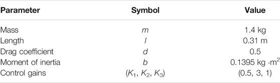
TABLE 1. Parameters used to simulate the fish robot system, based on the experimental testbed.

FIGURE 3

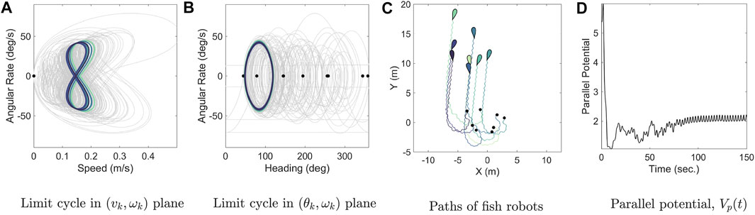
FIGURE 3. Simulation of Eq. 8 with parallel formation control Eq. 17 and N =8 identical fish. The black circular markers in (A–C) indicate the simulation states. The last 10 s of the limit cycle in (A) and (B) are shown with colored lines. The parallel potential Eq. 13 in (D) shown for 150 s.

3.2 Circular Formations

The parallel formation control Eq. 17 is based on the forward swimming control Eq. 9; however, a desired heading was not prescribed, but rather the average heading emerged through interactions among agents depending on their initial conditions. Similarly, a circular formation control is proposed here that drives the fish robots to continuously adjust their heading at a known average rate, while aligning the center position of the nominal circles to an (average) consensus value. Virtual fish can be introduced to achieve a reference heading or position (Sepulchre et al., 2007, 2008). Consider the following circular formation potential inspired by Eq. 5:

$V_c\left(t,\mathit{r},\mathit{\theta },\mathit{\omega }\right)=\frac{1}{2}{\mathit{\omega }}^{\mathrm{T}}\mathit{\omega }-K_2{\mathit{\gamma }}^{\mathrm{T}}\mathbf{1}+\frac{1}{2}{K}_3⟨\mathit{c},L\mathit{c}⟩,(19)$

where $\mathit{\gamma }={[{\gamma }_1,\dots ,{\gamma }_k]}^{\mathrm{T}}$ with γ_k(t) = cos(θ_k − ω₀t) and K₂, K₃ > 0. The time-derivative of V_c along trajectories of Eq. 12 is

${\dot{V}}_c\left(t,\mathit{r},\mathit{\theta },\mathit{\omega }\right)={\dot{\mathit{\omega }}}^{\mathrm{T}}\mathit{\omega }-K_2{\dot{\mathit{\gamma }}}^{\mathrm{T}}\mathbf{1}+K_3⟨\dot{\mathit{c}},L\mathit{c}⟩,(20)$

where ${\dot{\mathit{\gamma }}}^{\mathrm{T}}\mathbf{1}=-{\sum }_{k=1}^N\sin ({\theta }_k-{\omega }_{0}t)({\omega }_k-{\omega }_0),$ and ${\dot{\mathit{\omega }}}^{\mathrm{T}}\mathit{\omega }$ is given in Eq. 15.

When averaged over time, the motion of a fish robot resembles that of a self-propelled particle. Recall that the reference circle center for a self-propelled particle is $c_k=r_k+v_0{\omega }_0^{-1}i{e}^{i{\theta }_k}$. Since the average swimming speed of the robots is bK₁/ml (Lee et al., 2019), then by setting v₀ = bK₁/ml, the parameter ω₀ may be chosen to yield an average turn rate and reference circle with radius $|v_0{\omega }_0^{-1}|$. However, ω₀ should be sufficiently small to ensure that ω_k switches signs along the limit-cycle so that the robots flap. The third term in Eq. 20, evaluated along trajectories of Eq. 12, is

$\langle \dot{\mathit{c}},L\mathit{c}\rangle =\sum _{k=1}^N\left[\frac{l}{d}{\omega }_k-\frac{v_0}{{\omega }_0}\right]{\omega }_k\langle e^{i{\theta }_k},L_k\mathit{c}\rangle .(21)$

Therefore Eq. 20 may be rewritten as

$\begin{array}{cc}\hfill {\dot{V}}_c\left(t,\mathit{r},\mathit{\theta },\mathit{\omega }\right)& =\sum _{k=1}^N\left[\left(-a{\omega }_k^3-b^{-1}{u}_k\right){\omega }_k\right.\hfill \\ \hfill & +K_2\sin \left({\theta }_k-{\omega }_{0}t\right)\left({\omega }_k-{\omega }_0\right)\hfill \\ \hfill & +K_3\left.\left[\frac{l}{d}{\omega }_k-\frac{v_0}{{\omega }_0}\right]{\omega }_k⟨e^{i{\theta }_k},L_k\mathit{c}⟩\right].\hfill \end{array}(22)$

Choosing the control

$\begin{array}{cc}\hfill u_k=& b\left(-K_1{\omega }_k+K_2\sin \left({\theta }_k-{\omega }_{0}t\right)\right.\hfill \\ \hfill & +K_3\left[\frac{l}{d}{\omega }_k-\frac{v_0}{{\omega }_0}\right]⟨e^{i{\theta }_k},L_k\mathit{c}⟩),\hfill \end{array}(23)$

the derivative Eq. 22 becomes

$\begin{array}{cc}\hfill {\dot{V}}_c=& \sum _{k=1}^N\left[\left(-a{\omega }_k^2+K_1\right){\omega }_k^2-K_2{\omega }_0\sin \left({\theta }_k-{\omega }_{0}t\right)\right]\hfill \\ \hfill \le & \sum _{k=1}^N\left[\left(-a{\omega }_k^2+K_1\right){\omega }_k^2\right.\left.+K_2|{\omega }_0|\right].\hfill \end{array}(24)$

Thus, ${\dot{V}}_c<0$ outside ${\mathrm{\Omega }}_c=\{(\mathit{\theta },\mathit{\omega })\in {\mathbb{T}}^N\times {\mathbb{R}}^N:{\omega }_k^2\le (K_1+\sqrt{K_1^2+4a{K}_2|{\omega }_0|})/2a\forall k\in \mathcal{V}\}$, which implies the system is driven to a bounded set containing the desired limit cycle. The K₃ term in Eq. 23 biases the torque to align the reference circles, whereas the remaining terms produce a flapping motion with a given average turn rate. Although Eq. 24 remains negative for any positive K₃, this gain must be chosen sufficiently small to ensure flapping. As with Eq. 17, the feedback control Eq. 23 relies only on relative-state measurements between agents and does not include feedback linearization of the agents’ dynamics.

The circular formation feedback control Eq. 17 is numerically illustrated by simulating Eq. 8 with parameters from Table 1 and using ω₀ = 0.05 rad/s. The simulation was conducted for ten minutes to demonstrate circular motion. Figure 4A shows all N robots converge to the same limit cycle in the (v_k, ω_k) plane. The orbits in Figure 4B resemble the limit cycle in Figure 3B; however, due to the time-varying term in Eq. 19, they translate along the perimeter of the phase cylinder. The net result is motion along a circle whose center position is determined by the initial conditions of the agents (Figure 4C). Since the oscillating centers are aligned when all robots have identical position and phase, the controller drives all the robots to one side of the circle. In ongoing work, we seek to stabilize symmetric circular formations (Sepulchre et al., 2007; Sepulchre et al., 2008), which evenly distribute the agents around the formation. The circular potential exhibits low and high frequency oscillations (Figure 4D), which correspond to motion around the reference circle and flapping, respectively.

FIGURE 4

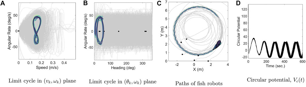
FIGURE 4. Simulation of Eq. 8 with circular formation control Eq. 23 and N = 8 identical fish. Black circular markers in (A–D) indicate initial simulation states. The last 5 s of the simulation are shown with colored lines in (A) and (B), and the last 90 s in (C).

4 Experimental Results

This section describes the implementation of the parallel formation control law Eq. 17 on a school of robotic fish and experimental results. First, the experimental testbed used in this work is briefly described. Next, results from system identification experiments are presented that provide parameters for a model of the reaction wheel dynamics. Based on this model, an inner-loop linear-quadratic-Gaussian (LQG) controller is implemented to track a desired reference torque generated from the formation control law using the onboard motor’s angular velocity measurements. Lastly, results from a series of in-water experiments demonstrating the parallel formation control are presented.

4.1 Experimental Testbed

The fish-inspired soft robots used in the experiments (Figure 1) are each driven by a Pololu 12 V DC motor (with a 4.4 to 1 gear ratio) that oscillates a reaction wheel located at each robot’s center of mass. Each fish robot measures its orientation with an onboard BNO055 inertial measurement unit (IMU) sensor that features a built-in extended Kalman filter. A micro-SD card is used to store sensor data and a 900 MHz xBee radio enables each fish robot to communicate with a ground station and other fish robots on the water’s surface. Each fish robot performs onboard sensor processing and control with a Teensy 3.2 microcontroller. For a more detailed discussion of the fish robots’ design, refer to (Lee et al., 2019).

The experiments were conducted in a 367,000 gallon water tank at the Neutral Buoyancy Research Facility at the University of Maryland, College Park. An overhead camera is mounted above the experimental area to record the true position of each robotic fish; however, the position data is not used in real time by the fish for formation control. Instead, during formation control experiments, each robot exchanges orientation data from their onboard IMU with other fish in the school using the xBee radios. Since the position of each robotic fish is not computed in real-time, an invariant complete communication graph was used in the experiments; whereas, a proximity-based communication graph was used in simulation.^AT The overhead camera images are post-processed after each experiment to visualize the trajectory of each robotic fish. The image processing uses MATLAB’s built-in corner/object detection based on a minimum eigenvalue algorithm (The MathWorks, 2019) and a built-in constant velocity Kalman filter for object tracking. Since all of the sensing and control law computations occur onboard, the school of robotic fish are a self-contained system when performing formation control experiments. The block diagram in Figure 5 gives an overview of the experimental testbed.

FIGURE 5

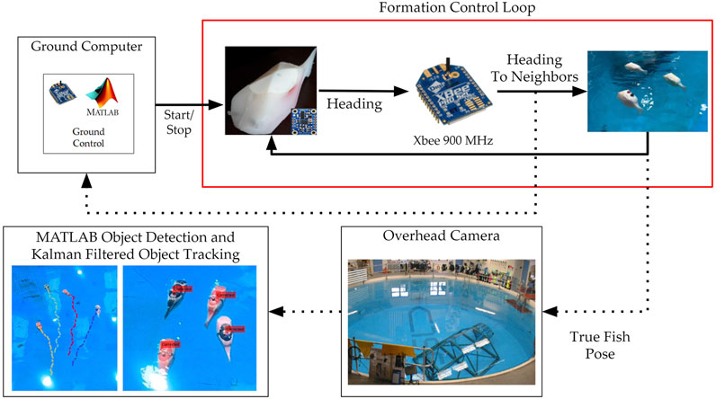
FIGURE 5. Block diagram of the experimental testbed. Since all of the sensing and control law computations occur onboard, the school of robotic fish are a closed self-contained system when performing parallel formation control experiments.

The nonlinear control laws Eq. 17 or Eq. 23 generate a reference torque command that steers the fish robots to their respective formations. However, this torque cannot be commanded directly since the control input into the reaction wheel system is the voltage applied to the DC motor generated by the motor driver and Teensy micro-controller. Furthermore, the only available measurement is the angular velocity of the motor’s shaft measured by an encoder. Thus, to track the reference torque a linear-quadratic-Gaussian (LQG) controller and estimator was implemented. The LQG controller assumes the following motor dynamics (Kim, 2017):

$\begin{array}{ccc}\hfill \mathrm{\Lambda }& =\hfill & \mu \frac{di}{dt}+Ri+e\hfill \end{array}(25)$

$\begin{array}{ccc}\hfill e& =\hfill & K_e\dot{\psi }\hfill \end{array}(26)$

$\begin{array}{ccc}\hfill \tau & =\hfill & K_{\tau }i\hfill \end{array}(27)$

$\begin{array}{ccc}\hfill J\ddot{\psi }& =\hfill & \tau -{\zeta }_m\dot{\psi },\hfill \end{array}(28)$

where Λ is the voltage input, R is the motor’s electrical resistance, μ is the inductance, i is the current, e is the motor’s back electromotive force (EMF), $\dot{\psi }$ is the angular rate of the output shaft, J is the sum of inertias between the reaction wheel and motor’s output shaft, τ is the torque applied by the motor, ζ_m is the internal damping friction applied to output shaft, and K_e and K_τ are the motor’s generator and torque constants, respectively. To identify the values of the DC motor and reaction wheel parameters, a series of system identification experiments were conducted, as described next.

The resistance of the motor R was measured directly with an ohm meter, and the sum of the motor and reaction wheel inertias J was approximated using analytical expressions for the moment of inertia of a cylinder about its axis of symmetry with a known mass and diameter. To determine the motor generator constant K_e, substitute Eq. 26 into Eq. 25 and examine the system at steady current state, i.e., di/dt = 0. Solving for $\dot{\psi }$ yields

$\dot{\psi }=\frac{1}{K_e}\left(\mathrm{\Lambda }-Ri\right).(29)$

Using a Rigol DP711 power supply and quadrature encoder attached to the motor’s output shaft, a series of constant voltages were applied to the motor. For each voltage, the current through the motor and the angular velocity of the output shaft at steady state were recorded. A linear regression was used to determine the quantity 1/K_e, which is the slope of the line in Eq. 29 and Figure 6A.

FIGURE 6

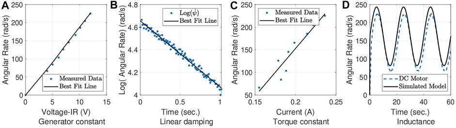
FIGURE 6. Experimental data used to identify motor-reaction wheel dynamics: Panels (A–C) are used to infer the values of the generator constant, linear damping, and torque constant through linear regression. Panel (D) compares the motor’s simulated and actuated response with a best guessed value of the inductance.

The internal frinction coefficient ζ_m was found by setting the torque to zero, i.e., τ = 0 in Eq. 28, and solving the resulting differential equation to obtain

$\ln \left(\dot{\psi }\left(t\right)\right)=-\frac{{\zeta }_m}{J}t+\ln \left(\dot{\psi }\left(0\right)\right),(30)$

where $\dot{\psi }(0)$ is the initial shaft angular velocity. Notice that Eq. 30 is a linear equation that describes $\ln (\dot{\psi })$ as a function of time. A similar technique as described previously can be used to find − ζ_m/J from a time-history of torque-free motor data. To identify the damping parameter, the motor was initialized with a constant nonzero angular velocity and the input voltage was removed. The motor’s angular velocity was recorded as it decays under internal friction. As before, a linear regression was used to determine the slope − ζ_m/J in Eq. 30 from Figure 6B and, hence, ζ_m can be inferred since J is known.

To determine the torque constant K_τ, substitute Eq. 27 into Eq. 28 at steady state ($\dot{\psi }$ constant) and solve for $\dot{\psi }$ to obtain

$\dot{\psi }=\frac{K_{\tau }}{{\zeta }_m}i.(31)$

By repeating the procedure used to determine K_e, using the value of ζ_m, the value of K_τ is found from the slope K_τ/ζ_m in Eq. 31 and Figure 6C.

Since the inductance μ only plays a role in the transient response of the motor, which are sufficiently fast, we estimate this parameter heuristically. The simulated response of the motor to a sinusoidal voltage input is visually compared to the actual response of the motor under the same input. The process is repeated while adjusting the value of μ to obtain a similar response, as shown in Figure 6D.

Lastly, the motor was found to exhibit a range of deadband voltages near zero that resulted in the motor being unresponsive. To determine the range of this deadband, a series of incrementally increasing voltages were applied to the motor, giving an approximate deadband range of ± 4V. The parameter values determined through this system identification process are summarized in Table 2.

TABLE 2

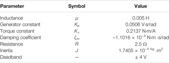
TABLE 2. Motor parameters identified through system identification for the Pololu 12 V DC Motor (with 4.4 to 1 gear ration) and reaction wheel.

4.2 DC Motor Torque Tracking Controller

To implement the LQG torque controller and state estimator for the DC motor, convert Eqs 25–28 into state space form where $\mathit{q}={\left[\tau ,\dot{\psi }\right]}^T$ denotes the states of the motor and the output is $\mathrm{\Upsilon }=\dot{\psi }$. The continuous-time state space equations take the form

$\dot{\mathit{q}}=\mathit{A}\mathit{q}+\mathit{B}\mathrm{\Lambda }(32)$

$\mathrm{\Upsilon }=\mathit{C}\mathit{q}(33)$

where

$\mathit{A}=\left[\begin{array}{cc}\hfill -\frac{R}{\mu }\hfill & \hfill -\frac{K_e{K}_{\tau }}{\mu }\hfill \\ \hfill \frac{1}{J}\hfill & \hfill -\frac{{\zeta }_m}{J}\hfill \end{array}\right],\mathit{B}=\left[\begin{array}{c}\hfill \frac{K_{\tau }}{\mu }\hfill \\ \hfill 0\hfill \end{array}\right],\text{and}\mathit{C}=\left[\begin{array}{cc}\hfill 0\hfill & \hfill 1\hfill \end{array}\right].(34)$

For implementation onboard the micro-controller, the continuous system Eqs 32, 33 is converted into a discrete-time system (with an addition of torque process noise and heading measurement noise):

${\mathit{q}}_{k+1}=\mathbf{\Phi }{\mathit{q}}_k+\mathbf{\Gamma }{\mathrm{\Lambda }}_k+\mathit{\xi }{w}_k(35)$

${\mathrm{\Upsilon }}_k=\mathit{C}{\mathit{q}}_k+{\eta }_k,(36)$

where (Crassidis and Junkins, 2011)

$\mathbf{\Phi }=e^{\mathit{A}\mathrm{\Delta }t},\mathbf{\Gamma }=\left({\int }_0^{\mathrm{\Delta }t}{e}^{\mathit{A}\tau }d\tau \right)\mathit{B},\mathit{\xi }=\left[\begin{array}{c}\hfill 1\hfill \\ \hfill 0\hfill \end{array}\right],(37)$

k is an integer indexing the discrete state, Δt = 100Hz is the time-step of the microcontroller, w_k is zero-mean, Gaussian, additive process noise with variance ${\sigma }_w^2$, and η_k is zero-mean, Gaussian, additive measurement noise with variance ${\sigma }_{\eta }^2$. We adopt the standard approach outlined in (Crassidis and Junkins, 2011) and (Brown and Hwang, 1997) to implement a discrete-time Kalman filter for the system Eqs 35, 36. The estimated state ${\widehat{\mathit{q}}}_k$ is used in a linear-quadratic-regulator (LQR) feedback control law of the form ${\mathrm{\Lambda }}_k={\mathit{\kappa }}^T({\mathit{q}}_d-{\widehat{\mathit{q}}}_k)$, where the κ is a gain matrix found by solving the discrete-time algebraic Riccati equation and q_d are the desired state values. Numerical values used in the LQG controller and estimator design are given in Table 3.

TABLE 3

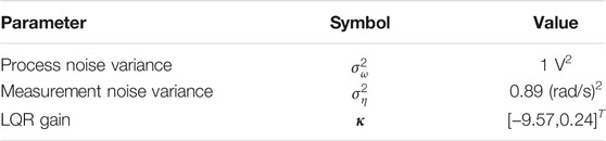
TABLE 3. Parameters used in a LQG controller and estimator.

To evaluate the LQG torque controller/estimator, the control law Eq. 9 was used to generate a reference torque for a step input change in desired heading. The performance of the torque tracking controller is shown in Figure 7A, and the heading trajectory of the fish robot during this experiment is examined in the next section.

FIGURE 7

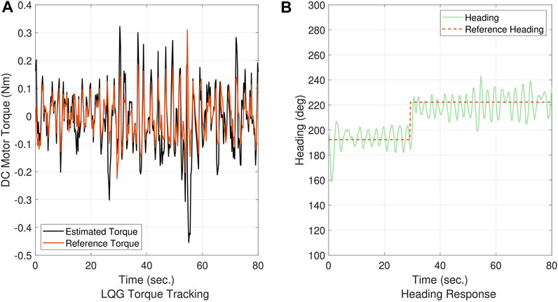
FIGURE 7. Experimental data from a closed loop heading controller Eq. 9: (A) the reference torque produced by Eq. 9 and the estimated torque from the LQG controller. (B) fish robot’s closed loop heading response to a step input reference heading.

4.3 Heading Control Experimental Results

We first examine the accuracy of the closed-loop directional controller Eq. 9, where θ_d is a desired heading. After testing Eq. 9 on a single robotic fish, we found that the DC motor’s deadband does not allow the average heading to completely converge to θ_d. When the fish robot’s heading is close to the desired heading, the voltage required to close the gap is too small and falls within the dead zone making the motor unresponsive. The accuracy of Eq. 9 is limited on our testbed due to this voltage deadband, but can also be mitigated by choice of the values of the nonlinear control gains K₁ and K₂. In both Eq. 9 and Eq. 17, increasing the value of K₂ makes the control laws more sensitive to relative heading errors and increases the torque required to minimize the error. Similarly K₁ amplifies the torque and, therefore the voltage input required to keep the fish swimming. Tuning these control gains increases the accuracy of the aforementioned control laws. The experimental results of this test with a step input for θ_d is shown in Figure 7B. The fish robot’s heading oscillates about a desired heading with a small persistent error between the average and desired headings. The control gains used in this experiment are K₁ = 0.5 and K₂ = 7.

4.4 Parallel Formation Experimental Results

To validate the theoretical results of the parallel formation control law Eq. 17, the results from six experiments are presented. The fish robots’ micro-controller uses IMU measurements for the heading and xBee radios for communication within the school. An overhead camera observes the positions of each fish robot; these were not used by the school during the experiments.

Four fish robots were initialized with random initial positions and orientations at the beginning of each parallel formation control experiment (implemented with gains K₁ = 3 and K₂ = 5). Consensus was achieved by the four fish with a small phase shift (up to 20 degrees) of the mean heading for each fish. This offset may be attributed to excess noise in angular velocity measurements and the aforementioned voltage dead zone. An example heading time-history from one of the experiments is shown in Figure 8A.

FIGURE 8

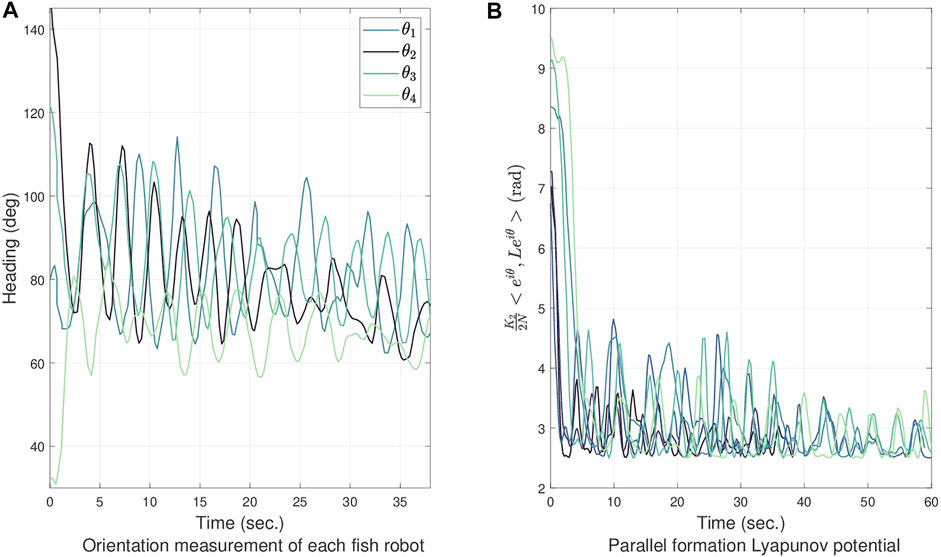
FIGURE 8. Parallel formation control onboard sensor data: (A) orientation measurements from onboard IMU for each fish robot while achieving a parallel formation. (B) experimental parallel formation misalignment potential computed for six independent experiments.

The excess noise in the angular velocity measurements caused large spikes to appear when computing the Lyapunov potential Eq. 13 from experimental data. Thus, to illustrate the convergence of this potential, the $\frac{1}{2}{\mathit{\omega }}^T\mathit{\omega }$ term was removed, leaving only the heading alignment term $\frac{K_2}{2N}<e^{i\theta },L{e}^{i\theta }>$ plotted in Figure 8B for each of the six experiments. As mentioned in Section 3, the potential function does not decrease completely to zero when consensus is achieved because each robot converges to a different phase on the limit cycle.

An example trajectory of the fish robots in Figure 9A and the Supplementary Material S1 shows the fish robots achieving consensus and swimming in a parallel formation. However, since the ground truth orientations of the fish robots are not used, errors in the IMU measurements sometimes cause a subset of the school to swim in a different direction than the rest of the school, as shown in Figure 9B. The error in IMU measurements may be caused by an erroneous calibration or magnetic anomalies in the water tank interfering with the onboard magnetometer.

FIGURE 9

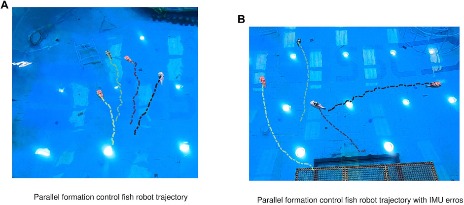
FIGURE 9. Parallel formation control of fish robot ground truth trajectory: (A) school of robotic fish swimming in a parallel formation. (B) errors affect the IMU of one fish causing to swim in a different direction than the rest of the school.

5 Conclusion

Nonlinear control laws are proposed that stabilize parallel and circular formations in a model of N planar fish robots. The control design approach extends prior work on collective motion of self-propelled particles to a school of robotic fish with Chaplygin sleigh dynamics. The feedback control laws rely only on relative-state measurements between agents that interact according to a connected, undirected, communication graph and do not include feedback linearization of the agents’ dynamics. Implementing the parallel control law on a testbed of fish robots required conducting system identification experiments to characterize the motor dynamics and designing a torque tracking motor controller and estimator. Numerical simulations and experiments on a school of robotic fish demonstrate the proposed approach. In ongoing work, we seek to model the fluid interactions between fish robots and instrument the robotic fish with pressure sensors to exploit the hydrodynamic benefits of close-proximity swimming.

Data Availability Statement

The raw data supporting the conclusion of this article will be made available by the authors, without undue reservation.

Author Contributions

DP, AW, and PG contributed to conception and design of the study. AT performed the experiments and analyzed the experimental data. AT and AW wrote the experimental sections of the manuscript. All authors contributed to manuscript revision, read, and approved the submitted version.

Funding

ONR Grant No. 115239289 and NSF Grant No. 1756179.

Conflict of Interest

The authors declare that the research was conducted in the absence of any commercial or financial relationships that could be construed as a potential conflict of interest.

Publisher’s Note

All claims expressed in this article are solely those of the authors and do not necessarily represent those of their affiliated organizations, or those of the publisher, the editors and the reviewers. Any product that may be evaluated in this article, or claim that may be made by its manufacturer, is not guaranteed or endorsed by the publisher.

Supplementary Material

The Supplementary Material for this article can be found online at: https://www.frontiersin.org/articles/10.3389/fcteg.2021.782121/full#supplementary-material

References

Berlinger, F., Gauci, M., and Nagpal, R. (2021). Implicit Coordination for 3D Underwater Collective Behaviors in a Fish-Inspired Robot Swarm. Sci. Robot 6 (50), eabd8668. doi:10.1126/scirobotics.abd8668

PubMed Abstract | CrossRef Full Text | Google Scholar

Bloch, A. M. (2003). “The Chaplygin Sleigh,” in Nonholonomic Mechanics and Control (New York, NY: Springer), 25–29.

Google Scholar

Brinón-Arranz, L., Seuret, A., and Canudas-de Wit, C. (2014). Cooperative Control Design for Time-Varying Formations of Multi-Agent Systems. IEEE Trans. Automatic Control. 59 (8), 2283–2288. doi:10.1109/TAC.2014.2303213

CrossRef Full Text | Google Scholar

Brown, R. G., and Hwang, P. Y. (1997). Introduction to Random Signals and Applied Kalman Filtering: With MATLAB Exercises and Solutions. New York, NY: Wiley, 214–220.

Google Scholar

Cao, Y., and Ren, W. (2012). “Finite-Time Consensus for Single-Integrator Kinematics with Unknown Inherent Nonlinear Dynamics under a Directed Interaction Graph,” in American Control Conf, 1603–1608. doi:10.1109/acc.2012.6315428

CrossRef Full Text | Google Scholar

Cao, Y., Yu, W., Ren, W., and Chen, G. (2013). An Overview of Recent Progress in the Study of Distributed Multi-Agent Coordination. IEEE Trans. Ind. Inf. 9 (1), 427–438. doi:10.1109/tii.2012.2219061

CrossRef Full Text | Google Scholar

Chopra, N. (2012). Output Synchronization on Strongly Connected Graphs. IEEE Trans. Automat. Contr. 57 (11), 2896–2901. doi:10.1109/tac.2012.2193704

CrossRef Full Text | Google Scholar

Crassidis, J. L., and Junkins, J. L. (2011). Optimal Estimation of Dynamic Systems. New York, NY: CRC Press.

Google Scholar

Diestel, R. (2000). “The Basics,” in Graph Theory (New York, NY: Springer), 1–28.

Google Scholar

Free, B., Patnaik, M. K., and Paley, D. A. (2017). “Observability-Based Path-Planning and Flow-Relative Control of a Bioinspired Sensor Array in a Karman Vortex Street,” in American Control Conf, Seattle, WA, May 24–26, 2017, 548–554. doi:10.23919/acc.2017.7963010

CrossRef Full Text | Google Scholar

Free, B. A., Lee, J., and Paley, D. A. (2020). Bioinspired Pursuit with a Swimming Robot Using Feedback Control of an Internal Rotor. Bioinspir. Biomim. 15 (3), 035005. doi:10.1088/1748-3190/ab745e

PubMed Abstract | CrossRef Full Text | Google Scholar

Horn, R. A., and Johnson, C. R. (1990). Matrix Analysis. New York, NY: Cambridge University Press.

Google Scholar

Jain, A., and Ghose, D. (2019). Trajectory-Constrained Collective Circular Motion with Different Phase Arrangements. IEEE Trans. Automatic Control. 65 (5), 2237–2244. doi:10.1109/TAC.2019.2940233

CrossRef Full Text | Google Scholar

Justh, E. W., and Krishnaprasad, P. S. (2004). Equilibria and Steering Laws for Planar Formations. Syst. Control. Lett. 52 (1), 25–38. doi:10.1016/j.sysconle.2003.10.004

CrossRef Full Text | Google Scholar

Kelly, S. D., Fairchild, M. J., Hassing, P. M., and Tallapragada, P. (2012). “Proportional Heading Control for Planar Navigation: The Chaplygin Beanie and Fishlike Robotic Swimming,” in American Control Conf, Montreal, QC, June 27–29, 2012, 4885–4890. doi:10.1109/acc.2012.6315688

CrossRef Full Text | Google Scholar

Kim, S.-H. (2017). Electric Motor Control: DC, AC, and BLDC Motors. Amsterdam, Netherlands: Elsevier.

Google Scholar

Lee, J., Free, B., Santana, S., and Paley, D. A. (2019). “State-Feedback Control of an Internal Rotor for Propelling and Steering a Flexible Fish-Inspired Underwater Vehicle,” in American Control Conf, Philadelphia, PA, July 10–12, 2019, 2011–2016. doi:10.23919/acc.2019.8814908

CrossRef Full Text | Google Scholar

Li, T., Fu, M., Xie, L., and Zhang, J.-F. (2011). Distributed Consensus with Limited Communication Data Rate. IEEE Trans. Automat. Contr. 56 (2), 279–292. doi:10.1109/tac.2010.2052384

CrossRef Full Text | Google Scholar

Moreau, L. (2005). Stability of Multiagent Systems with Time-Dependent Communication Links. IEEE Trans. Automat. Contr. 50 (2), 169–182. doi:10.1109/tac.2004.841888

CrossRef Full Text | Google Scholar

Napora, S., and Paley, D. A. (2013). Observer-Based Feedback Control for Stabilization of Collective Motion. IEEE Trans. Contr. Syst. Technol. 21 (5), 1846–1857. doi:10.1109/tcst.2012.2205252

CrossRef Full Text | Google Scholar

Olshevsky, A. (2015). Linear Time Average Consensus on Fixed Graphs∗∗This Work Was Supported by NSF Award CMMI-1463262. IFAC-PapersOnLine 48 (22), 94–99. doi:10.1016/j.ifacol.2015.10.313

CrossRef Full Text | Google Scholar

Paley, D. A. (2007). Cooperative Control of Collective Motion for Ocean Sampling with Autonomous Vehicles. Ph.D. thesis. Princeton, NJ: Princeton University.

Google Scholar

Paley, D. A. (2008). “Cooperative Control of an Autonomous Sampling Network in an External Flow Field,” in IEEE Conf. Decision and Control, Cancun, Mexico, December 9–11, 2008 (IEEE), 3095–3100. doi:10.1109/cdc.2008.4739077

CrossRef Full Text | Google Scholar

Paley, D. A. (2009). Stabilization of Collective Motion on a Sphere. Automatica 45 (1), 212–216. doi:10.1016/j.automatica.2008.06.012

CrossRef Full Text | Google Scholar

Pollard, B., Fedonyuk, V., and Tallapragada, P. (2019). Swimming on Limit Cycles with Nonholonomic Constraints. Nonlinear Dyn. 97 (4), 2453–2468. doi:10.1007/s11071-019-05141-z

CrossRef Full Text | Google Scholar

Ren, W., and Beard, R. W. (2005). Consensus Seeking in Multiagent Systems under Dynamically Changing Interaction Topologies. IEEE Trans. Automat. Contr. 50 (5), 655–661. doi:10.1109/tac.2005.846556

CrossRef Full Text | Google Scholar

Ren, W., Beard, R. W., and Atkins, E. M. (2007). Information Consensus in Multivehicle Cooperative Control. IEEE Control. Syst. Mag. 27 (2), 71–82. doi:10.1109/MCS.2007.338264

CrossRef Full Text | Google Scholar

Reynolds, C. W. (1987). Flocks, Herds and Schools: A Distributed Behavioral Model. SIGGRAPH Comput. Graph. 21 (4), 25–34. doi:10.1145/37402.37406

CrossRef Full Text | Google Scholar

Scardovi, L., Sarlette, A., and Sepulchre, R. (2007). Synchronization and Balancing on the N-Torus. Syst. Control. Lett. 56 (5), 335–341. doi:10.1016/j.sysconle.2006.10.020

CrossRef Full Text | Google Scholar

Sepulchre, R., Paley, D. A., and Leonard, N. E. (2007). Stabilization of Planar Collective Motion: All-To-All Communication. IEEE Trans. Automat. Contr. 52 (5), 811–824. doi:10.1109/tac.2007.898077

CrossRef Full Text | Google Scholar

Sepulchre, R., Paley, D. A., and Leonard, N. E. (2008). Stabilization of Planar Collective Motion with Limited Communication. IEEE Trans. Automat. Contr. 53 (3), 706–719. doi:10.1109/tac.2008.919857

CrossRef Full Text | Google Scholar

[Dataset] The MathWorks (2019). Track a Face in Scene.

Google Scholar

Vicsek, T., Czirók, A., Ben-Jacob, E., Cohen, I., and Shochet, O. (1995). Novel Type of Phase Transition in a System of Self-Driven Particles. Phys. Rev. Lett. 75, 1226–1229. doi:10.1103/physrevlett.75.1226

PubMed Abstract | CrossRef Full Text | Google Scholar

Yu, X., and Liu, L. (2017). Cooperative Control for Moving-Target Circular Formation of Nonholonomic Vehicles. IEEE Trans. Automat. Contr. 62 (7), 3448–3454. doi:10.1109/tac.2016.2614348

CrossRef Full Text | Google Scholar

Wenwu Yu, W., Guanrong Chen, G., Ming Cao, M., and Kurths, J. (2010). Second-order Consensus for Multiagent Systems with Directed Topologies and Nonlinear Dynamics. IEEE Trans. Syst. Man. Cybern. B 40 (3), 881–891. doi:10.1109/tsmcb.2009.2031624

CrossRef Full Text | Google Scholar

Yu, X., Liu, L., and Feng, G. (2018). Distributed Circular Formation Control of Nonholonomic Vehicles without Direct Distance Measurements. IEEE Trans. Automat. Contr. 63 (8), 2730–2737. doi:10.1109/tac.2018.2790259

CrossRef Full Text | Google Scholar

Zhang, Y., and Tian, Y.-P. (2009). Consentability and Protocol Design of Multi-Agent Systems with Stochastic Switching Topology. Automatica 45 (5), 1195–1201. doi:10.1016/j.automatica.2008.11.005

CrossRef Full Text | Google Scholar

Zhang, F., Washington, P., and Paley, D. A. (2016). “A Flexible, Reaction-Wheel-Driven Fish Robot: Flow Sensing and Flow-Relative Control,” in American Control Conf, Boston, MA, July 6–8, 2016, 1221–1226. doi:10.1109/acc.2016.7525084

CrossRef Full Text | Google Scholar

Zhang, Z., Yang, T., Zhang, T., Zhou, F., Cen, N., Li, T., et al. (2021). Global Vision-Based Formation Control of Soft Robotic Fish Swarm. Soft Robotics 8 (3), 310–318. doi:10.1089/soro.2019.0174

PubMed Abstract | CrossRef Full Text | Google Scholar