A high-precision fault diagnosis method for photovoltaic arrays considering the effect of missing data

With the increasing penetration of photovoltaic (PV) systems into power grids, the accurate diagnosis of PV array health has become critical for ensuring the stable operation of power systems. To address the problem of missing data collected from PV arrays and reduced diagnostic accuracy when compound faults occur, we propose a high-precision fault diagnosis model for PV arrays based on Tucker decomposition-sparrow search algorithm (SSA)-Informer-MSCNet. First, a tensor Tucker decomposition-based method is proposed to complete the missing data. Then, an informer network is employed to fully extract the global features. Next, an MSCNet model is proposed to extract multi-scale key features. The SSA is then used to optimize the model’s global parameters. We use the fault dataset to realize the missing data completion and fault diagnosis tests of PV arrays. The results show that the complementary algorithm thus designed has some accuracy. The proposed fault diagnostic model is able to achieve 98.73% and 97.46% accuracy in case of single and compound faults in PV arrays, respectively, and maintains 96.12% accuracy at 30 dB noise.

1 Introduction

With the acceleration of global energy transition, photovoltaic (PV) power generation is a core component of clean renewable energy. Its installed capacity has shown explosive growth (Agoua et al., 2018; Parenti et al., 2024). However, PV systems are exposed long-term to complex outdoor environments (e.g., high temperature, sand, dust, and rain). The frequent occurrence of problems such as aging of PV equipment, module failure, and inverter failure can lead to large losses in system power generation (Ahadi et al., 2016a; Ahadi et al., 2016b; Peng et al., 2024). This seriously affects the reliability and economy of energy supply.

With the rapid development of artificial intelligence technology, deep learning is widely being used in PV fault diagnosis (Emanuele et al., 2021; Ren et al., 2025). In response to the above problems, a series of studies have been launched into PV fault diagnosis. Saravanan et al. (2025) proposed the Binary Greylag Goose Optimization (BGGO) methodology for diagnosing six shadows and other single faults in 9 × 9 panel PV arrays. Wang et al. (2019) proposed a fault diagnosis algorithm based on support vector machine (SVM) to achieve short circuit, open circuit, and shadowing fault detection in PV arrays by researching the I-V characteristic curves of faulty PV arrays. Guo et al. (2025) proposed a neural network model incorporating multi-channel one-dimensional convolution to capture multi-scale information to improve feature representation; they then used LSTM, AdaBoost, and logistic regression methods to construct a stacked model to categorize a single fault type of PV arrays. Gong et al. (2024) proposed a multi-source information fusion network (MSIFN) and then used the multi-strategy fusion whale optimization algorithm (MSFWOA) to optimize the global parameters with good diagnostic results in three types of noise experiments at 15 dB, 25 dB, and 30 dB. Lu et al. (2019) transformed the time series currents and voltages of PV arrays into two-dimensional electrical time series diagrams to visualize the characteristics of the time series data; they then proposed a convolutional neural network structure incorporating multiple convolutional layers and multiple pooling layers for PV array fault diagnosis. Xi et al. (2021) proposed a sparse representation of the Fisher discriminant dictionary learning (FDDL) method to diagnose PV array faults, interline faults, open-circuit faults, and partially shaded faults. Liu et al. (2019) proposed a primitive clustering method based on expansion and erosion theory to diagnose PV array faults by using an unsupervised learning method which does not need to pre-determine the number of clusters and has high adaptability and effectiveness under multi-dimensional meteorological data input. Lu et al. (2021) proposed a dual-channel convolutional neural network and designed a novel feature selection structure to improve the accuracy of PV fault diagnosis.

However, PV equipment operation can result in missing data due to factors such as blocked communication, environmental factors, and poor inverter quality. Existing fault diagnosis methods based on PV operation data do not account for the above problem of missing data in actual working conditions. The long-term operation of PV equipment can lead to wear and tear in multiple areas. Multiple damages from extreme weather (strong winds/rainstorms/lightning strikes) can also cause PV failures. In addition, when multiple small faults are not dealt with in time, they can easily develop into compound faults.

All of the above studies diagnose for a single fault type of PV. However, there has been no research into fault detection for PV equipment composite faults. Therefore, a PV equipment fault diagnosis method based on the Tucker decomposition-SSA-Informer-MSCNet model is proposed to accurately identify multiple composite faults in PV arrays. This will promote the development of smart grids and the construction of digital grids.

2 PV array failure analysis and causes of missing data

2.1 Causes of missing data collected from PV equipment

Typically, PV power plants monitor real-time voltage, current, and power along with environmental data such as temperature and irradiance. For fault detection, performance evaluation, or maintenance, this study establishes a practical PV simulation platform to collect operational data. The hardware components include PV panels, resistance boxes, temperature sensors, and electricity meters.

The PV data acquisition platform established here operates as a remote data collection system. During PV system testing and analysis, simulated datasets that are collected may experience data gaps due to a number of reasons. (1) Equipment failure or configuration errors: malfunctions in electricity meters or sensors may prevent data collection during specific periods. (2) Trigger desynchronization: asynchronous triggering signals between multiple devices (e.g., light sources and acquisition systems) may cause data misalignment or loss. (3) Irradiation instability: fluctuations in natural sunlight or unstable output from artificial light sources may interrupt measurements or trigger anomalies. (4) Temperature drift: significant component temperature changes during prolonged measurements can distort data. Without real-time temperature compensation, data within specific ranges may become invalid or distorted. (5) Component defects: hidden cracks, poor soldering, or cell failures may cause open circuits or short circuits within specific voltage/current ranges, interrupting data collection. (6) Data transmission errors: signal interference, communication blockages, or poor connections in wired/wireless transmission systems may cause data loss. (7) Operational errors: incorrect device calibration (leading to distorted low-current data), loose wiring, or poor probe contact may cause measurement interruptions.

When missing data occurs due to the above factors, repeating the measurement or repairing the equipment will waste time and resources Therefore, it is necessary to fill in the missing data of PV arrays.

2.2 PV array fault cause analysis and simulation

Long-term PV operation induces array failures such as short circuits, aging, shading, and cell degradation due to equipment wear and environmental stressors. Undetected minor faults propagate into multiple simultaneous failures through insufficient detection sensitivity and delayed intervention. These compound faults critically compromise power system stability. We simulated PV array failures using actual equipment. Figure 1 shows a schematic diagram of the measurement principle.

Figure 1

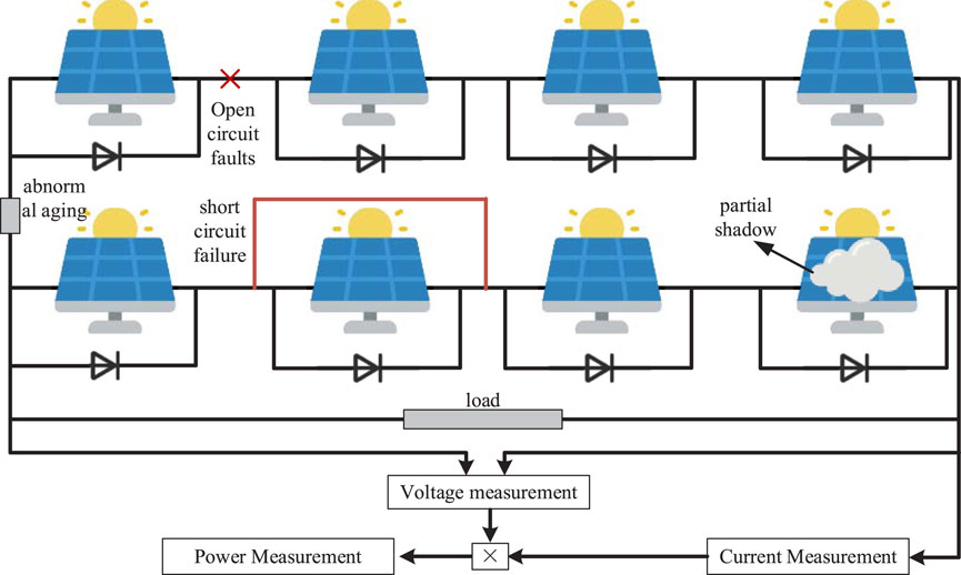
Figure 1. PV fault simulation structure.

Currently, the characteristics and causes of PV faults are widely agreed (Liu and Wu, 2025). (1) Aging faults are mainly due to the wear and tear of PV arrays caused by long operation time, which can be realized here by changing the resistance value. (2) Short circuit is the phenomenon of shorting at different points in the PV string, which can be realized by controlling the shunt resistance. (3) Localized shading refers to the fact that some modules are not able to receive sunlight due to shading by external objects, which leads to uneven output current of PV modules and reduces the overall power generation efficiency. This can be studied by controlling the input irradiance. (4) Open-circuit faults are caused by false soldering, desoldering, or breakage, which can be realized by controlling the respective branching structure. When two or more faults occur, they evolve into compound faults.

The data collected on PV operating voltage, current, power, and irradiance and temperature were obtained from an actual simulation platform consisting of eight PV modules connected in series and parallel. The model includes two series units, each comprising four PV modules connected in series. Thus, the total array configuration is 4 series × 2 parallel. Through fault simulation, operational data for various typical faults in the PV array were obtained and annotated under standard operating conditions.

3 Diagnosis of PV faulty arrays based on Tucker decomposition-SSA-informer-MSCNET models

3.1 Tucker decomposition and structure tensor based missing data recovery method for PV array acquisitions

PV data such as power (P), voltage (V), current (I), irradiance intensity, and timestamps represent typical high-dimensional data. Tensors, as computational tools capable of handling high-dimensional data, possess an inherent spatial structure. We use a Hankel tensor that can effectively improve data recovery accuracy (Yang et al., 2025). Taking the PV power data as an example, the MDT technique is used to construct the Hankel tensor.

We first designed a folding transformation operator as shown in Equation 1:

$fol{d}_{\left(\tau ,L-\tau +1\right)}:R^{\tau \left(L-\tau +1\right)}\to R^{\tau \times \left(L-\tau +1\right)}(1)$

—where $\tau$ is the delay window size, L is the vector length of PV data collection, and fold represents the fold operator.

Photovoltaic data acquisition requires standard delay transformation (also known as “Hankification”) to obtain the Hank form matrix, as shown in Equation 2:

$H_{\tau }\left(v\right)=fol{d}_{\left(\tau ,L-\tau +1\right)}\left(\delta x\right)=\left(\begin{array}{cccc}{x}_1& x_2& \cdots & x_{L-\tau +1}\\ x_2& x_3& \cdots & x_{L-\tau +2}\\ ⋮& ⋮& \ddots & ⋮\\ x_{\tau }& x_{\tau +1}& \cdots & x_L\end{array}\right)\in R^{\tau \times \left(L-\tau +1\right)}(2)$

—where x is the input PV data sequence, and $\delta \in {\left\{0,1\right\}}^{\tau \left(L-\tau +1\right)\times L}$ is a repetition matrix that satisfies (Equation 3)

$vec\left(H_{\tau }\left(v\right)\right)=\delta x(3)$

Then, the matrices are subjected to stacking operation to change into Hankel tensors.

The Hankel tensor filling model based on Tucker decomposition is established as shown in Equation 4:

$\underset{\mathcal{G},\mathcal{U},\mathcal{V},\mathcal{Y}}{\min }\frac{1}{2}{‖{\mathcal{P}}_{\mathrm{\Omega }}\times \left({\mathcal{H}}_{\mathcal{T}}\left(\mathcal{X}\right)-{\mathcal{H}}_{\mathcal{T}}\left(\mathcal{G}{\times }_1\mathcal{U}{\times }_2\mathcal{V}{\times }_3\mathcal{Y}\right)\right)‖}_F^2+\frac{\lambda }{2}\left({‖\mathcal{G}‖}_F^2+{‖\mathcal{U}‖}_F^2+{‖\mathcal{V}‖}_F^2+{‖\mathcal{Y}‖}_F^2\right)(4)$

—where ${\mathcal{P}}_{\mathrm{\Omega }}$ is the index of the non-missing data consisting of 0 and 1, ${\mathcal{H}}_{\mathcal{T}}\left(\mathcal{X}\right)$ is the original tensor, ${\mathcal{H}}_{\mathcal{T}}\left(\mathcal{G}{\times }_1\mathcal{U}{\times }_2\mathcal{V}{\times }_3\mathcal{Y}\right)$ is the reconstruction tensor, $\lambda$ is the regularization coefficient, $\mathcal{G}$ is the core tensor, and $\mathcal{U}$、$\mathcal{V}$、 $\mathcal{Y}$ are the factor matrices.

The alternating least squares method is used to solve the problem. Denoting the objective function as f, the partial derivatives for the core tensor $\mathcal{G}$ are given as Equation 5:

$\frac{\partial f}{\partial \mathcal{G}}=-P_{\mathrm{\Omega }}\left({\mathcal{H}}_{\mathcal{T}}\left(\mathcal{X}\right)-{\mathcal{H}}_{\mathcal{T}}\left(\mathcal{G}{\times }_1\mathcal{U}{\times }_2\mathcal{V}{\times }_3\mathcal{Y}\right)\right){\times }_1{\mathcal{U}}^T{\times }_2{\mathcal{V}}^T{\times }_3{\mathcal{Y}}^T+\lambda \mathcal{G}(5)$

The partial derivation of the factor matrix $\mathcal{U}$ is given as Equation 6:

$\frac{\partial f}{\partial \mathcal{U}}=-P_{\mathrm{\Omega }}({\mathcal{H}}_{\mathcal{T}}\left(\mathcal{X}\right)-{\mathcal{H}}_{\mathcal{T}}\left({\mathcal{U}\mathcal{G}\left(\mathcal{Y}\otimes \mathcal{V}\right)}^T\right)\left(\mathcal{Y}\otimes \mathcal{V}\right){\mathcal{G}}^T+\lambda \mathcal{U}(6)$

Similarly, the factor matrices $\mathcal{V}$ and $\mathcal{Y}$ have the same form. Alternate solving is performed.

After obtaining the final solved Hankel, the complete data are output after passing through the delayed inverse transformation, as shown in Equation 7:

$H_{\tau }^{†}\left({\mathcal{X}}^{\prime }\right)=unfol{d}_{\left(\tau ,L-\tau +1\right)}\left(\mathcal{X}\right)\times \left\{S^{†}\right\}(7)$

—where $S^{†}={\left(S^{T}S\right)}^{-1}{S}^T$ is the Moore–Penrose pseudo-inverse transformation, and $unfol{d}_{\left(\tau ,L-\tau +1\right)}$ is the inverse operation.

3.2 Feature extraction method based on Informer-MSCNET

The Informer network outperforms the Transformer network in long time-series feature extraction. The model also uses an encoder–decoder architecture, where the encoder converts the input information into dense vectors of fixed dimensions and extracts features from the elements in order to generate a mapping of the features (Zhou et al., 2021). The Informer model mainly consists of an input representation, an encoder, and a decoder, the structure of which is shown in Figure 2.

Figure 2

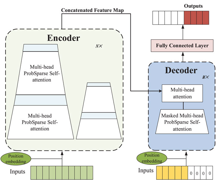
Figure 2. Informer structure diagram.

The core of the Informer model consists of a probabilistic sparse self-attention mechanism and distillation.

The main effect of the probabilistic sparse self-attention mechanism is to make key focus only on the first n queries with high relevance, as shown in Equation 8:

$\mathrm{Pr}ob=soft\max \left(\frac{\stackrel{-}{Q}{K}^T}{\sqrt{d}}\right)V(8)$

—where softmax (·) stands for the normalization operation, V stands for the value matrix, K^T stands for the transpose of the key matrix, and d is the input dimension. $\stackrel{-}{Q}$ is a sparse matrix containing only the first n queries.

The use of the Informer network can better capture the global information in the long-term operation data of PV equipment. This will enable the extraction of global features.

Current PV fault diagnosis methods exhibit limited noise robustness due to inadequate multi-scale feature extraction capabilities. This study proposes MSCNet to simultaneously achieve granular local channel feature extraction and adaptive multiscale feature fusion.

First, based on the given input feature F, global max pooling and global average pooling operations are performed, as shown in Equation 9:

$\begin{array}{l}{F}_{avg}=AvgPool\left(F\right)\\ F_{\max }=MaxPool\left(F\right)\end{array}(9)$

In the formula, AvgPool (·) represents average pooling calculation, and MaxPool (·) represents maximum pooling calculation.

Then, after nonlinear mapping through the fully connected layer, the final output is obtained through a gating mechanism, as shown in Equation 10:

$F^{\prime }=sigmoid\left(MLP\left(F_{Avg}\right)+MLP\left(F_{\mathit{Max}}\right)\right)(10)$

In the formula, sigmoid (·) represents the activation function, and MLP (·) represents multilayer linear layer computation.

Meanwhile, another branch first expands the number of channels and solves the gradient vanishing problem through the convolution layer, normalization layer, and ReLU activation function, as shown in Equation 11:

$F_u=\text{Re}LU\left(BN\left(Conv\left(F\right)\right)\right)(11)$

In the formula, ReLU(·) represents the activation function, BN(·)the normalization layer, and Conv (·) the convolution operation.

Then, we used the MSDC module to extract multiscale features, as shown in Equation 12:

$\begin{array}{l}{F}_{u1}=\text{Re}LU\left(BN\left(DW{C}_{1\times 1}\left(F_u\right)\right)\right)\\ F_{u2}=\text{Re}LU\left(BN\left(DW{C}_{3\times 3}\left(F_u\right)\right)\right)\\ F_{u3}=\text{Re}LU\left(BN\left(DW{C}_{5\times 5}\left(F_u\right)\right)\right)\end{array}(12)$

In the formula, DWC(·) stands for depthwise separable convolution.

Since depthwise separable convolutions ignore the relationships between channels, a channel shuffling operation is performed, as shown in Equation 13:

$F_o=ChannelShuffle\left(F_{u1}+F_{u2}+F_{u3}\right)(13)$

In the formula, channelshuffle (·) refers to channel recombination operation, and F_u1, F_u2, and F_u3 are the outputs after deep separable convolution.

Finally, we merged the two branches and obtained the final result through the fully connected layer, as shown in Equation 14:

$Out=MLP\left(F^{\prime }+F^{″}\right)(14)$

In the formula, Out is the final output.

MSCNet can capture the relationships between features in different channels of PV data. By recalibrating the weights of feature channels, the model can more effectively fuse multichannel information and improve overall feature representation capabilities. In our study, MSCNet is embedded after the convolutional pooling layer of the Informer encoder for feature enhancement. The MSCNet module enhances important features and suppresses irrelevant or redundant features by adaptively adjusting the weights of each channel feature in the PV data. This mechanism enhances the model’s sensitivity to key features of PV array fault signals, thereby improving the accuracy of PV fault diagnosis in noisy environments.

The final global model of the Informer-MSCNet network is shown in Figure 3.

Figure 3

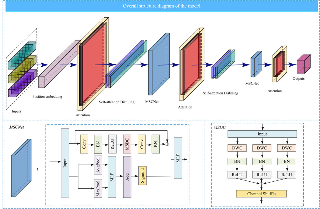
Figure 3. General model architecture diagram.

3.3 Global parameter optimization based on the sparrow optimization algorithm

The SSA algorithm is a mathematical model built by simulating the foraging and anti-predatory behavior of sparrows (Xue and Shen, 2020). Its core idea is that sparrows are divided into two groups: discoverers and joiners. The discoverers mainly find food and lead other sparrows. The joiners follow the discoverers to get food. In addition, the algorithm is designed with vigilantes, which are mainly responsible for monitoring the surroundings and alerting when danger is detected.

The steps of the algorithm are as follows:

1. initialize the population and related parameters and calculate the fitness value of the initial population;

2. update the finder position, as shown in Equation 15:

$X_{i,j}^{t+1}=\left\{\begin{array}{l}{X}_{i,j}^t·\exp \left(\frac{-i}{\alpha ·ite{r}_{\max }}\right)\text{\hspace{0.5em}if }{R}_2<ST\\ X_{i,j}^t+Q·L\text{\hspace{1em}if }{R}_2>ST\end{array}\right.(15)$

—where R₂ is the warning value, and ST is the safety value. When R₂<ST, it means it is safe. When R₂>=ST, it indicates that there is some safety risk and it is necessary to move to a safe area.

3. Updating of accessionist positions, as shown in Equation 16:

$X_{i,j}^{t+1}=\left\{\begin{array}{l}Q·\exp \left(\frac{X_{worst}^t-X_{i,j}^t}{i^2}\right)\text{\hspace{0.5em}if }i>\raisebox{1ex}{$n$}\!\left/ \!\raisebox{-1ex}{$2$}\right.\\ X_p^{t+1}+\left|X_{i,j}^t-X_p^{t+1}\right|·A^{+}·L\text{\hspace{1em}otherwise}\end{array}\right.(16)$

—where X_p is the position of the optimal explorer in the sparrow population, X_worst is the current global worst position, and n is the population size. A is a 1×d matrix with random amplitude 1 or −1 for each element, where A⁺ is defined as Equation 17:

$A^{+}=A^T{\left(A{A}^T\right)}^{-1}(17)$

4. In case of danger, there is a need to update the location, in a timely manner, of the sparrows that are aware of the danger, as shown in Equation 18:

$X_{i,j}^{t+1}=\left\{\begin{array}{l}{X}_{best}^t+\beta ·\left|X_{i,j}^t-X_{best}^t\right|\mathrm{i}f{f}_i>f_g\\ X_{i,j}^t+K·\left(\frac{\left|X_{i,j}^t-X_{worst}^t\right|}{\left(f_i-f_w\right)+\epsilon }\right)\mathrm{i}f{f}_i=f_g\end{array}\right.(18)$

—where X_best is the current global optimal position, β is a parameter whose main function is to control the step size and obeys a normal distribution with mean 0 and variance 1, K is a random number in [−1,1], f is the fitness value, f_g and f_w are the current optimal and worst fitness values, respectively, and ε is a constant to avoid the denominator being 0.

5. Determine whether the stop condition is satisfied; if so, output the optimal sparrow position; otherwise, continue to update the finder position.

4 Experimental analysis

We conducted a simulation experiment to collect real PV data in a city in northern China. The simulation system comprised real PV modules, a resistor box, an electricity meter, temperature sensors, an irradiance meter, and other equipment. Data were collected at 15-min intervals, resulting in a final dataset containing 4320 × 5 sampling points. Furthermore, the ambient temperature in the dataset ranged from 25.47 °C to 34.69 °C, and the irradiance ranged from 527.25 W/m² to 765.14 W/m². This was based on the simulation under different environmental conditions and operating states and to establish the PV array simulation fault data set. Then, based on pytorch1.8 framework, a python3.10 program is written.

For convenience of presentation, all fault types and labels used in this paper are shown in Table 1.

Table 1

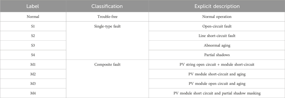
Table 1. Fault types and labeling.

4.1 PV array acquisition data missing fill experiment

The simulated data were subjected to missing simulation, and two common scenarios—random missing and continuous missing of current data—were set up. Cubic spline interpolation, KNN (Song et al., 2025), SVM (Chao et al., 2021), and low-rank matrix filling (Miao and Kou, 2022) were selected as comparison methods. RSE was adopted as the evaluation index of different methods. The formulas are as shown in Equation 19:

$\text{RSE}=\frac{{‖{\mathcal{X}}_{\mathrm{\Omega }}^{\prime }-{\mathcal{X}}_{\mathrm{\Omega }}‖}_{\mathrm{F}}}{{‖{\mathcal{X}}_{\mathrm{\Omega }}‖}_{\mathrm{F}}}\times 100\%(19)$

where $\mathcal{X}$ is the original complete tensor, ${\mathcal{X}}^{\prime }$ is the post-completion complete tensor, and ||·||_F denotes the F-paradigm.

In randomized missing recovery experiments, a single random missing datum is arbitrarily selected. We set the proportion of missing data in steps of 5% and step from 5% to 50% for 50 sets of experiments. The experimental results are shown in Figure 4.

Figure 4

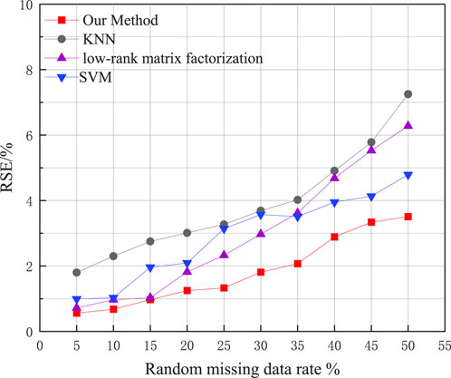
Figure 4. Completion effect of random missing data.

It can be seen that using this method has good results for the current missing data filling collected from PV arrays. Specifically analyzed, in the case of 50% random missing rate, the RSE is 3.51% using our method. This method is 3.74%, 2.77%, and 1.28% lower than KNN, low-rank matrix padding, and SVM, respectively, which shows the good results of the proposed algorithm.

Since we use an actual remote measurement system, continuous data loss occurs when problems such as remote device communication failures, unstable connections, and sensor failures occur. We considered data filling experiments with current data loss rates of 5%, 10%, 15%, 20%, 25%, and 30%. The comparison results are as follows.

As analyzed from this figure, the RSE of the proposed algorithm in this study is 5.27% with 30% continuous missing ratio. The KNN, low-rank matrix, and SVM-based algorithms are 9.93%, 10.28%, and 7.98%, respectively. Moreover, the RSE of this study’s algorithm is lower than that of the comparison algorithms, regardless of any percentage where the continuous missing rate is set.

4.2 Photovoltaic array single-fault comparison experiment

This study simulates four single types of fault: short-circuit, aging, open circuit, and localized shadow; these are prone to occur in PV arrays under real working conditions. CNN (Xie et al., 2022), SVM (Koloko et al., 2022), TCN (Yating et al., 2021), Transformer (Khalil et al., 2024), and Informer (Ma et al., 2025) are selected for comparison tests. Classification accuracy, check accuracy, and recall are used as the evaluation indexes of single fault diagnosis accuracy. As shown in Equations 20–22.

$Acc=\frac{1}{N}{\displaystyle \sum _{i=1}^N}Ac{c}_i=\frac{1}{N}{\displaystyle \sum _{i=1}^N}\frac{T{P}_i+T{N}_i}{T{P}_i+T{N}_i+F{P}_i+F{N}_i}(20)$

$P=\frac{T{P}_i}{T{P}_i+F{P}_i}(21)$

$R=\frac{T{P}_i}{T{P}_i+F{N}_i}(22)$

where N is the total number of categories, ACC_i represents the classification accuracy of faults in category i, TP_i and TN_i denote the number of samples correctly classified by the model as category i and non-i, respectively, and FP_i and FNi denote the number of samples incorrectly classified as category i and non-i. The confusion matrix is shown in Table 2.

Table 2

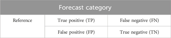
Table 2. Confusion matrix.

In the case of the consecutively missing 30% of data, the experimental results of fault detection accuracy after obtaining the SVM method of complementation and after using our method are shown in Tables 3 and 4.

Table 3

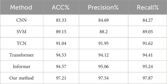
Table 3. Comparison of the effect of PV single-fault detection after using SVM complementation.

Table 4

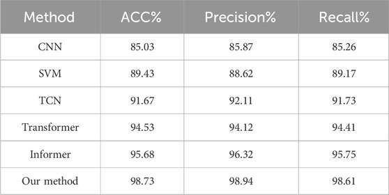
Table 4. Comparison of photovoltaic single-fault detection effect after complementation using the method of this study.

It can be seen that the accuracy of data filling has an impact on the accuracy of different fault detection algorithms. Among these, the most influential is the CNN algorithm, which can improve the ACC by 1.7%. When using the fault detection algorithm in this study, the fault detection ACC is improved by 1.52%, the check accuracy is improved by 1.4%, and the recall rate is improved by 1.24%. Therefore, it is able to demonstrate the impact of data filling accuracy on PV array fault diagnosis.

We further analyzed the fault diagnosis accuracy of different algorithms. The algorithm we propose is effective in several evaluation indexes. The Informer model is effective in PV array single-fault detection with ACC of 95.68%, while the model built here has an ACC of 98.73%—an improvement of 3.05% compared to the ACC of the Informer model. At the same time, the checking accuracy percentage (precision) is 98.92% compared with Informer, Transformer, TCN, SVM, CNN improvements of 2.62%, 3.82%, 6.83%, 10.32%, and 13.07%, respectively. The recall of the model we propose is 98.61%, compared with Informer, Transformer, TCN, SVM, and CNN at 2.86%, 3.2%, 6.88%, 9.44%, and 13.35%, respectively. The effectiveness of our method in single PV fault diagnosis is thus demonstrated.

4.3 Performance evaluation and analysis of single-fault diagnosis models under the influence of noise

In the actual operation of PV equipment, noise is an indispensable component in real measurement data. In this study, 30 dB and 40 dB of noise are added to simulate the real measurement environment for comparison tests. The comparison algorithm selects the Informer and Transformer models that perform well in the single fault of PV array. The relevant results are shown in Figures 6, 7.

As can be seen from Figure 5, our algorithm performs well in the simulated real scenario, with an average recognition accuracy of 98.4%—2.8% and 5% higher than that of Informer and Transformer, respectively—further illustrating that our algorithm has good ability to be applied in engineering.

Figure 5

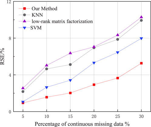
Figure 5. Completion effect of continuous missing data.

The results of the associated fault classification when adding 40 dB of noise are shown in the heat map below.

From Figures 6, 7 it can be seen that in the face of 40 dB noise, the proposed algorithm in this study only reduces the recognition accuracy of localized shadow faults and aging faults of PV equipment by nearly 2% and 1%, respectively, compared with when 30 dB noise is applied. For other types of faults, the recognition accuracy is basically unchanged. Transformer and Informer are affected to different degrees. For specific analysis, the accuracy of the Informer model in recognizing open circuit, short circuit, and aging decreases by nearly 2%, 3%, and 6%, respectively, compared with when 30 dB noise is applied, while the accuracy of the Transformer model in recognizing normal operation, open circuit, short circuit, and aging decreases by nearly 6%, 5%, 1%, and 5%, respectively, compared with when 30 dB noise is applied. This demonstrates the good robustness of our algorithm, and further shows that it has good application in engineering.

Figure 6

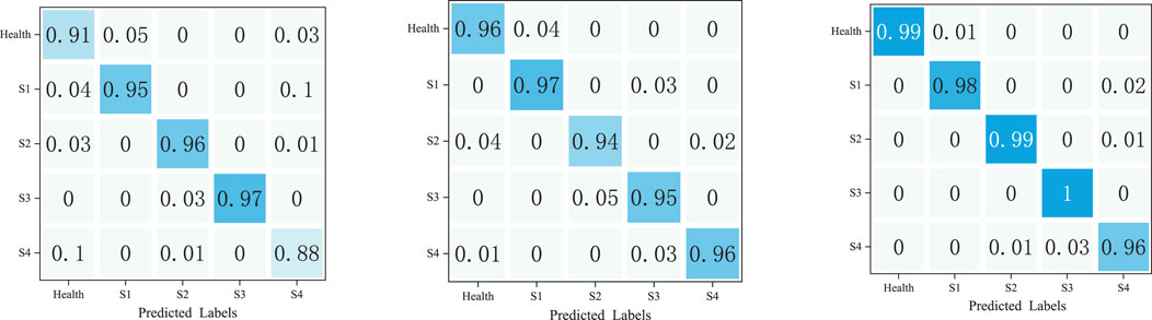
Figure 6. Single-fault identification accuracy of PV devices under 30 dB noise.

Figure 7

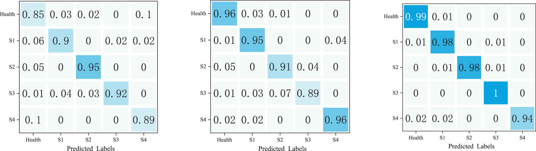
Figure 7. Single-fault identification accuracy of PV devices under 40 dB noise.

4.4 Performance evaluation and analysis of composite fault diagnosis models under the influence of noise

When a single fault is not removed in time, it evolves into a compound fault. According to the model proposed here, several experiments were carried out based on the addition of four composite fault types, and the experimental results were obtained as shown in Figure 8.

Figure 8

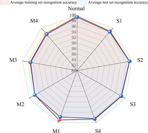
Figure 8. Photovoltaic complex fault training set and test set accuracy.

It can be seen that the PV fault diagnosis model we propose still has good recognition accuracy after adding the four new faults. Specifically analyzed, both the average training and test set accuracy still have good recognition accuracy for single-PV fault diagnosis accuracy. In the case of composite faults, the average training set accuracy of M1-fault-type recognition is 98.92%, the average test set accuracy is 97.46%, and the average training and test set accuracy of M2, M3, and M4 faults are close to each other. Therefore, the algorithm proposed in this study still has high diagnostic accuracy for PV arrays with compound faults.

We also simulated a real engineering scenario when a compound fault occurs. A noise of 30 dB was added to the occurrence of the compound fault. The experimental results we obtained are shown in Figure 9.

Figure 9

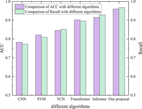
Figure 9. Composite fault recognition accuracy of different algorithms.

It can be seen that the ACC of the algorithm proposed in this paper is 96.12% with the addition of four composite faults and the addition of 30 dB of noise effects. It improves 4.61%, 5.9%, 11.51%, 13.96%, and 17.88% compared to Informer, Transformer, TCN, SVM, and CNN. The Recall algorithm proposed in this paper is 96.76% compared to the Informer, Transformer, TCN, SVM, CNN improvements of 3.9%, 7.19%, 11.6%, 15.72%, and 19.45%, respectively. This illustrates that our algorithm still shows effective and robust results under the occurrence of compound faults and the addition of 30 dB noise.

4.5 Ablation experiment

To validate the effectiveness of the proposed MSCNet, this section conducts ablation experiments. These comprehensively identify single and composite faults. The experimental results are shown in Figure 10 (the left figure shows TCN-Informer-SSA, and the right figure shows the proposed algorithm).

Figure 10

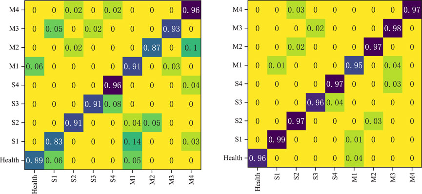
Figure 10. Heat map comparing ablation experiments.

As shown in the experimental results figure, the use of MSCNet significantly improves the detection accuracy of both single and composite faults in photovoltaic arrays. Overall, the accuracy of the algorithm proposed in this study for PV fault diagnosis exceeds 95%. In contrast, the TCN-Informer-SSA algorithm achieves an accuracy of over 95% only when identifying the health status of PV equipment and S4 faults, while its accuracy falls below 90% when identifying healthy PV equipment, S1 faults, and M2 faults. Specifically, when an S1-type fault occurs, the identification accuracy of the algorithm we propose is 0.99, while the TCN-Informer-SSA algorithm achieves only 0.83, which is 16% lower than our algorithm. This further validates the effectiveness of the MSCNet proposed here for multi-scale feature extraction.

5 Conclusion

This study proposes a photovoltaic (PV) fault diagnosis model based on Tucker decomposition-SSA-Informer-MSCNet. The model can effectively identify single and composite faults in PV arrays and withstand the influence of 30 dB and 40 dB noise. It has important application value in engineering practice and also has good diagnostic effects for composite faults. The specific conclusions are as follows.

1. This study proposes the Tucker decomposition method to fill missing data. It provides good data inputs to the subsequently constructed model, which is important for improving fault identification accuracy.

2. The Informer-MSCNet model is proposed to fully extract data features. By embedding MSCNet into the Informer network, multiscale key features were extracted, greatly improving fault diagnosis accuracy.

3. For the problem of many parameters of the Informer-MSCNet model, this study uses the sparrow search algorithm (SSA) to optimize the global parameters, thus accelerating the convergence of the model.

4. PV single fault and composite fault, containing 30 dB noise impact of data simulation and using the model we propose for PV array fault diagnosis experiments are shown to be effective by our results.

Data availability statement

The raw data supporting the conclusions of this article will be made available by the authors without undue reservation.

Author contributions

DL: Conceptualization, Data curation, Funding acquisition, Writing – review and editing, Software, Writing – original draft, Resources. XZ: Investigation, Supervision, Writing – review and editing, Methodology. CD: Validation, Writing – review and editing, Software, Supervision.

Funding

The author(s) declare that financial support was received for the research and/or publication of this article. This paper is supported by the project “Key Technology Research and Product Development of Digital Enhancement of New active Distribution Network with Source Network Load and Storage Coordination” of Beijing Fibrlink Communications Co., LTD. (Project number: 546826240038).

Conflict of interest

Authors DL, XZ, and CD were employed by Beijing Fibrlink Communications Co., LTD.

The authors declare that this study received funding from the project “Key Technology Research and Product Development of digital Enhancement of New active Distribution Network with Source Network load and storage Coordination” of Beijing Fibrlink Communications Co., LTD.(Project number:546826240038). The funder had the following involvement in the study: data collection and analysis,decision to publish.

Generative AI statement

The author(s) declare that no Generative AI was used in the creation of this manuscript.

Any alternative text (alt text) provided alongside figures in this article has been generated by Frontiers with the support of artificial intelligence and reasonable efforts have been made to ensure accuracy, including review by the authors wherever possible. If you identify any issues, please contact us.

Publisher’s note

All claims expressed in this article are solely those of the authors and do not necessarily represent those of their affiliated organizations, or those of the publisher, the editors and the reviewers. Any product that may be evaluated in this article, or claim that may be made by its manufacturer, is not guaranteed or endorsed by the publisher.

References

Agoua, X. G., Girard, R., and Kariniotakis, G. (2018). Short-term spatio-temporal forecasting of photovoltaic power production. IEEE Trans. Sustain. Energy 9 (2), 538–546. doi:10.1109/TSTE.2017.2747765

CrossRef Full Text | Google Scholar

Ahadi, A., Miryousefi Aval, S. M., and Hayati, H. (2016a). Generating capacity adequacy evaluation of large-scale, grid-connected photovoltaic systems. Front. Energy 10, 308–318. doi:10.1007/s11708-016-0415-9

CrossRef Full Text | Google Scholar

Ahadi, A., Hayati, H., Mitra, J., Abbasi-Asl, R., and Awodele, K. (2016b). A new method for estimating the longevity and degradation of photovoltaic systems considering weather states. Front. Energy 10, 277–285. doi:10.1007/s11708-016-0400-3

CrossRef Full Text | Google Scholar

Chao, T., Ziwei, Z., Yining, Z., Zhou, M., Peng, S., Shan, S., et al. (2021). Online monitoring data processing method of transformer oil chromatogram based on association rules. IEEJ Trans. Electr. Electron. Eng. 17(3):354–360. doi:10.1002/tee.23518

CrossRef Full Text | Google Scholar

Emanuele, S., Kumar, A. J., Ioannis, D., Valastro, S., Sanzaro, S., Mannino, G., et al. (2021). MAPbI3 Deposition by LV-PSE on TiO2 for photovoltaic application. Front. Electron. 2, 726171. doi:10.3389/felec.2021.726171

CrossRef Full Text | Google Scholar

Gong, B., An, A., Shi, Y., and Jia, W. (2024). Fault diagnosis of photovoltaic array with multi-module fusion under hyperparameter optimization. Energy Convers. Manag. 319 (2024), 118974. doi:10.1016/j.enconman.2024.118974

CrossRef Full Text | Google Scholar

Guo, F., Fu, W., Wang, Y., and Chen, J. (2025). Research on fault diagnosis method for photovoltaic array based on model fusion. Electr. Eng., 107, 8189–8199. doi:10.1007/s00202-025-02963-6

CrossRef Full Text | Google Scholar

Khalil, I. U., Ul Haq, A., and Islam, N. (2024). A deep learning-based transformer model for photovoltaic fault forecasting and classification. Electr. Power Syst. Res. 228. doi:10.1016/j.epsr.2023.110063

CrossRef Full Text | Google Scholar

Koloko, J. R. K., E, P., Wamkeue, R., and Melingui, A. (2022). Fault detection and classification of a photovoltaic generator using the BES optimization algorithm associated with SVM. Int. J. Photoenergy, 1, 14. doi:10.1155/2022/6841861

CrossRef Full Text | Google Scholar

Lu, X., Lin, P., Cheng, S., Fang, G., He, X., Chen, Z., et al. (2021). Fault diagnosis model for photovoltaic array using a dual-channels convolutional neural network with a feature selection structure. Energy Convers. Manag. 248 (2021), 114777. doi:10.1016/j.enconman.2021.114777

CrossRef Full Text | Google Scholar

Liu, Y., and Wu, Y. (2025). Fault diagnosis of photovoltaic modules: a review. Sol. Energy 293, 113489. doi:10.1016/j.solener.2025.113489

CrossRef Full Text | Google Scholar

Liu, S., Dong, L., Liao, X., Hao, Y., Cao, X., and Wang, X. (2019). A Dilation and erosion-based clustering approach for fault diagnosis of photovoltaic arrays. IEEE Sensors J. 19 (11), 4123–4137. doi:10.1109/JSEN.2019.2896236

CrossRef Full Text | Google Scholar

Lu, X., Lin, P., Cheng, S., Lin, Y., Chen, Z., Wu, L., et al. (2019). Fault diagnosis for photovoltaic array based on convolutional neural network and electrical time series graph. Energy Convers. Manag. 196 (2019), 950–965. doi:10.1016/j.enconman.2019.06.062

CrossRef Full Text | Google Scholar

Ma, S., Shi, S., Zhang, Y., and Gao, H. (2025). A High-precision method for detecting rolling bearing faultis in unmanned aerial vehicle based on improved 1DCNN-Informer model. Measurement 256, 118200. doi:10.1016/j.measurement.2025.118200

CrossRef Full Text | Google Scholar

Miao, J., and Kou, K. I. (2022). Color image recovery using low-rank Quaternion matrix completion algorithm. IEEE Trans. Image Process. 31, 190–201. doi:10.1109/TIP.2021.3128321

PubMed Abstract | CrossRef Full Text | Google Scholar

Parenti, M., Fossa, M., and Delucchi, L. (2024). A model for energy predictions and diagnostics of large-scale photovoltaic systems based on electric data and thermal imaging of the PV fields. Renew. Sustain. Energy Rev. 206, 114858. doi:10.1016/j.rser.2024.114858

CrossRef Full Text | Google Scholar

Peng, M., Feng, L., Zhang, S., and Zhao, W. (2024). Stable operating limits and improvement methods for hydropower and photovoltaic integration through MMC-HVDC systems. Front. Electron. 4, 1342795. doi:10.3389/felec.2023.1342795

CrossRef Full Text | Google Scholar

Ren, S., Yang, T., Luo, J., Wu, G., Mao, K., and Liu, B. (2025). Performance evaluation of photovoltaic scenario generation. Front. Phys. 13, 131534629–1534629. doi:10.3389/fphy.2025.1534629

CrossRef Full Text | Google Scholar

Saravanan, S., Senthil Kumar, R., Balakumar, P., and Prabaharan, N. (2025). Optimal power harvesting under partial shading: Binary Greylag Goose optimization for reconfiguration and Machine learning-Based fault diagnosis in solar PV arrays. Energy Convers. Manag. 333, 119808. doi:10.1016/j.enconman.2025.119808

CrossRef Full Text | Google Scholar

Song, J., Xu, H., Li, J., and Zhang, S. (2025). Demand-driven kNN classification. Knowledge-Based Syst. 327, 114090. doi:10.1016/j.knosys.2025.114090

CrossRef Full Text | Google Scholar

Wang, J., Gao, D., Zhu, S., Wang, S., and Liu, H. (2019). Fault diagnosis method of photovoltaic array based on support vector machine. Energy Sources, Part A Recovery, Util. Environ. Eff. 45 (2), 5380–5395. doi:10.1080/15567036.2019.1671557

CrossRef Full Text | Google Scholar

Xi, P., Lin, P., Lin, Y., Zhou, H., Cheng, S., Chen, Z., et al. (2021). Online Fault diagnosis for photovoltaic arrays based on Fisher Discrimination Dictionary learning for sparse representation. IEEE Access 9, 30180–30192. doi:10.1109/ACCESS.2021.3059431

CrossRef Full Text | Google Scholar

Xie, W., Li, Z., Xu, Y., Gardoni, P., and Li, W. (2022). Evaluation of different bearing fault Classifiers in Utilizing CNN feature extraction ability. Sensors 22, 3314. doi:10.3390/s22093314

PubMed Abstract | CrossRef Full Text | Google Scholar

Xue, J., and Shen, B. (2020). A novel swarm intelligence optimization approach: sparrow search algorithm. Syst. Sci. and Control Eng. 8 (1), 22–34. doi:10.1080/21642583.2019.1708830

CrossRef Full Text | Google Scholar

Yang, T., Liu, G., Wang, Y., Suo, S., Zhang, M., and Yang, Z. (2025). A tensor completion algorithm for missing user data in spot trading of electricity market. Comput. Electr. Eng. 122, 109988. doi:10.1016/j.compeleceng.2024.109988

CrossRef Full Text | Google Scholar

Yating, G., Wu, W., Qiongbin, L., Fenghuang, C., and Qinqin, C. (2021). Fault diagnosis for power Converters based on optimized Temporal convolutional network. IEEE Trans. Instrum. Meas. 70, 1–10. doi:10.1109/TIM.2020.3021110

PubMed Abstract | CrossRef Full Text | Google Scholar

Zhou, H., Zhang, S., Peng, J., Zhang, S., Li, J., Xiong, H., et al. (2021). Informer: beyond Efficient transformer for long sequence time-series forecasting. Proc. AAAI Conf. Artif. Intell. 35 (12), 11106–11115. doi:10.1609/aaai.v35i12.17325

CrossRef Full Text | Google Scholar