A novel simulation and supervised machine learning-based prediction framework to predict the total transportation and energy costs for single-family households

This paper focuses on predicting the total transportation and energy costs (TTEC) for single-family households. A system boundary consisting of grid-powered electricity (GE) and solar-powered electricity (SE) as energy inputs and transportation vehicles that include Gasoline Vehicles (GV) and Electric Vehicles (EV) as transportation methods for energy outputs is studied. A novel three-stage evaluation framework is proposed to predict the TTEC under varying single-family household parameters. In the first stage, an energy balance simulation model is proposed to estimate the TTEC for an individual household. In the second stage, the simulation model is run several times under varying parameters to develop synthetic data that is used as input for the third stage supervised machine learning (SML) models. In the third stage, numerous SML models are trained and tested to determine the best SML model that enables us to predict the TTEC with high accuracy. This best SML model can be used as a substitute for simulation model, thereby reducing the computation burden of running the simulation model for each new single-family household. A case study of single-family households in Central Texas in the US is used as an application of the framework. The results indicate that regression SML models are best in predicting the total costs with an adjusted R-squared of 99.13% and 98.88% on training and testing datasets, respectively. In addition, the parameter analysis of regression SML models suggests that the house size, number of GVs, number of EVs, EV and GV ownership costs, and solar implementation at households are the most important parameters to predict TTEC for single-family households. Counterintuitively, number of residents, GV and EV mileage, solar system size, battery capacity and peak solar hours are not significant parameters that contribute to TTEC prediction.

1 Introduction

Over the past few decades, gasoline vehicles (GVs) have dominated transportation for single-family households. While GVs are cost-effective, they emit significant greenhouse (GHG) gas emissions. In addition, increasing transportation needs of public, limitations in fuel prices, fluctuations in transportation fuel prices along with increasing public calls for sustainability initiatives have driven governments across the world to seek alternatives for GVs (Falahi et al., 2013; Jones et al., 2023; IEA, 2024). Consequently, electric vehicles (EVs) have emerged as an environmentally friendly option, with many governments offering tax incentives or subsidies to promote their adoption and make them more economically competitive with GVs. As EV technology advances and costs decrease, households are gradually integrating EVs into their transportation choices (Ajanovic, 2015). However, due to charging time challenges, EVs are often used for short-distance travel, leading to a mix of transportation methods at the household level, including all GV, a combination of GV and EV, or all EV, depending on preferences.

These varying transportation combinations also result in different energy requirements. For example, households with only GVs need both electricity for residential use and gasoline for transportation, while those with only EVs require electricity for both purposes. Therefore, selecting the optimal transportation mix is important for meeting energy needs efficiently.

Historically, single-family households have relied on grid-powered electricity (GE), which is typically generated from non-renewable sources, contributing to environmental harm. With the rise in EV usage, electricity demands have surged, increasing GHG emissions and straining the grid, sometimes causing blackouts during peak times. In response, governments worldwide have promoted solar-powered electricity (SE) as a renewable, eco-friendly supplement to GE, reducing pressure on the grid. Tax incentives and subsidies are now available for households that adopt solar energy. Thus, it is crucial for households to find the right balance between grid and solar power to meet their electricity demands effectively.

Given the wide variety of options available for single-family households for fulfilling their transportation and electricity needs, single-family households typically make their transportation and electricity requirement decisions based on total transportation and energy costs (TTEC). The TTEC for a typical single-family household depends on several parameters that include, but not limited to number of residents, house size, number of GVs, number of EVs, GV and EV ownership costs, solar system implemented at a household or not, and solar system size. Consequently, it is important to understand which are important factors that contribute to the estimation of the TTEC. A comprehensive review of literature raises three important research questions as there is still ambiguity in estimation of TTEC for different combinations for single-family households. These research questions include:

1. Is there really any significant difference in TTEC costs when different combinations of electricity inputs and transportation methods as energy outputs are considered for a single-family household?

2. Is there a methodology that can help to predict TTEC for single-family households with a variety of parameters?

3. What are the important factors that contribute to the prediction or estimation of the total costs for single-family households?

To address these research questions, in this study, we examine a holistic system that considers GE and SE systems as electricity inputs and EVs and GVs as transportation methods for energy outputs. Our study aims to predict the TTEC for any given single-family household with a specific set of input parameters. We propose a novel three-stage prediction framework in which we first develop an energy balance simulation model to estimate TTEC for individual single-family households. Then, in the second stage, we run the model several times with varying parameters and develop synthetic data to train supervised machine learning (SML) models. In the final stage, different SML are trained and tested to determine the best SML model that can be implemented in real-world for TTEC prediction. It is important to highlight that once the best SML is determined, running of simulation model can be eliminated as the SML model will serve as a substitute for simulation model that will automatically predict the TTEC with high degree of accuracy as that of simulation model, thereby reducing computational effort and complexity.

2 Literature review

Over the past decade, several studies have been conducted to compare the total cost of ownership for EVs and GVs. Wu et al. (2015) create a probabilistic simulation model to evaluate and contrast electric vehicles (EVs) with fuel-powered vehicles. They find that, while EVs are approaching conventional vehicles in terms of total cost of ownership, their performance superiority depends on a variety of favorable factors. Mitropoulos et al. (2017) conduct a life cycle cost analysis to compare ownership costs across conventional, hybrid, and electric vehicles. Their findings show that hybrid vehicles outperform both conventional and electric vehicles over a wide range of life cycle distances. However, a trade-off exists: for shorter life cycle distances, EVs are more advantageous, while conventional vehicles perform better over longer distances. Similar to Wu et al. (2015), Danielis et al. (2018) designs a probabilistic simulation model to compare the total cost of ownership between electric vehicles (EVs) and gasoline vehicles (GVs) considering both stochastic and non-stochastic factors. Unlike Wu et al. (2015), who expressed uncertainty about cost-competitiveness, Danielis et al. (2018) suggest that EVs could become cost-competitive with GVs if fuel prices continue to rise, and EV retail prices continue to decrease. Weldon et al. (2018) conducts an economic analysis of fuel vehicles and EVs using a decade of data, finding that EVs are already cost-competitive with fuel vehicles. However, this study notes that this competitiveness depends on multiple factors and recommends continuing government incentives to support EV adoption until the technology fully matures. Hassan et al. (2024) perform an economic analysis to calculate the cost of ownership per kilometer, finding that EVs have a lower per kilometer ownership cost compared to gasoline-powered cars, despite their higher upfront price and battery replacement costs. The per kilometer cost for EVs decreases further when electricity rates are favorable and clean car discounts are offered. Liu et al. (2021) compare ownership costs between electric and fuel vehicles using an economic model, finding that EVs tend to be more expensive than fuel vehicles. However, their study notes that EV ownership costs become comparable to those of fuel vehicles when EVs are driven shorter distances. While there are numerous studies comparing the total cost of ownership of GV and EV, their cost competitiveness is still ambiguous and questionable.

In recent years, the total cost of EV ownership compared to GVs has been assessed by using solar-generated electricity as the main source of energy for EV charging. Accordingly, several researchers have examined EVs and solar power as integrated systems. Coffman et al. (2017) perform a life cycle assessment for a single-family household, considering both grid and solar power alongside fuel and electric vehicles. The study reveals that EVs typically have higher ownership costs than GVs. However, with subsidies for EVs and incentives for photovoltaic (PV) systems, EV ownership can become more cost-effective than GVs. Fachrizal and Munkhammar (2020) developed a quadratic programming approach for communities in high-latitude regions, where photovoltaic power production is lower and EV travel distances are greater. Their findings suggest that EV smart charging schemes can help reduce the PV load in these high latitude areas. Cieslik et al. (2021) conducted an energy balance analysis to evaluate a single-family household system integrating solar power generation with an EV. Through various scenarios, the study found that using photovoltaic (PV) systems or solar energy can be economically viable for household power needs, including EV charging, in certain scenarios compared to others. Göhler et al. (2021) assessed a multifamily household powered by both grid and solar energy, using EVs for transportation. They developed a simulation model, and the findings show that the energy self-sufficiency of a multifamily building powered by photovoltaic (PV) systems drops from 100% to 91% when EV charging is factored in. Boström et al. (2021) created a simulation model to analyze the synergy between solar energy and EVs as supply-demand dynamics for the entire nation of Spain. This conceptual study investigates a scenario in which all vehicles are electric, and energy is exclusively generated from photovoltaic systems, resulting in a completely self-sufficient energy system. After conducting a series of simulations, the study concluded that solar energy could theoretically meet all the energy requirements for both EVs and residential needs in Spain, provided that EVs are also utilized as energy storage units. Liang et al. (2022) employed a difference-in-differences (DID) model at the community level, focusing on a system powered by both grid and solar energy for EV charging. Their research concludes that the combined adoption of photovoltaic systems and EVs reduces system loads more effectively than the adoption of EVs alone. Furthermore, photovoltaic solar systems provide considerable economic advantages to consumers who use EVs. Salles-Mardones et al. (2022) performed an economic assessment on single family households in Viña del Mar, Chile by considering both grid- and solar-based electricity supply for EV charging. Numerous scenarios for solar-based electricity generation based on with and without battery storage are studied. The study concludes that smaller photovoltaic systems with battery storage capacities can cost-effectively meet the electricity demands of EVs due to lower capital expenditure of implementing solar power. Martin et al. (2022) examined single-family households that utilized solar power for electricity and employed EVs for transportation. The study used empirical analysis, focusing on performance metrics related to EV charging demand met by photovoltaic (PV) systems and CO2 emissions. The results showed that photovoltaic systems could fulfill between 15% and 90% of the energy requirements for EVs, depending on household charging behaviors and the availability of battery storage. Kassem et al. (2023) conducted energy and economic assessments for single-family households in Northern Cyprus, focusing on solar energy to meet both residential and electric vehicle charging requirements. The findings suggest that, due to the ample solar radiation in Northern Cyprus, solar energy is both technically viable and economically feasible for fulfilling these needs. Furthermore, the study indicates that using EVs in conjunction with solar energy offers greater economic advantages compared to fuel-powered vehicles.

Even though several studies have been conducted, two important insights have been provided in literature:

1. When EVs and GVs total cost of ownership are compared, GV seems to be better than EV even though EV in recent years has been closing the cost-competitiveness with GV.

2. Solar-powered EV is better than GV, given the fact that numerous subsidies are available to both solar power installation and EV purchases.

However, these two notions are supported by literature with a caveat that several parameters or factors should fall in favor of EV for EV to outperform GV. The study of our literature raises three important research questions that need further investigation:

1. Is there really any significant difference in TTEC costs when different combinations of electricity inputs and transportation methods as energy outputs are considered for a single-family household?

2. Is there a methodology that can help to predict TTEC for single-family households with a variety of parameters?

3. What are the important factors that contribute to the prediction or estimation of the total costs for single-family households?

To address these research questions, in this study, we examine a holistic system that considers GE and SE systems as electricity inputs and EVs and GVs as transportation methods for energy outputs. Our study aims to predict the TTEC for any given single-family household with a specific set of input parameters. We propose a novel three-stage prediction framework in which we first develop an energy balance simulation model to estimate TTEC for individual single-family households. Then, in the second stage, we run the model several times with varying parameters and develop synthetic data to train supervised machine learning (SML) models. In the final stage, different SML are trained and tested to determine the best SML model that can be implemented in real-world for TTEC prediction. It is important to highlight that once the best SML is determined, running of simulation model can be eliminated as the SML model will serve as a substitute for simulation model that will automatically predict the TTEC with high degree of accuracy as that of simulation model, thereby reducing computational effort and complexity.

3 Materials and methods

This section presents the materials and methods used in the proposed study. We first define the scope of the system boundary used in this study and then present a novel three-stage prediction framework required to predict the TTEC for single-family households and determine important parameters that contribute significantly towards predicting TTEC. The three-stage prediction model consists of supervised machine learning (SML) models that are trained and tested by using the TTEC predictions of energy balance simulation model. While the energy balance simulation model is same as studies performed by Wu et al. (2015) and Danielis et al. (2018), the training and testing the SML models is the unique contribution of this paper to literature. The benefit of training and testing SML model is that it supplements the use of simulation model, thereby reducing the computation burden and allows the best SML model automatically predict TTEC with high degree of accuracy.

3.1 Scope of the system boundary

This research focuses on predicting TTEC for any given single-family households with any specific set of input parameters. Figure 1 presents a generic system boundary considered in this study. It consists of a single-family household that uses grid-powered electricity (GE) and Solar-powered electricity (SE) as energy inputs and gasoline vehicles (GVs) and electric vehicles (EVs) as transportation methods for energy output. The parameters considered in the study are limited to Central Texas region in US.

Figure 1

Figure 1. System boundary for a single-family household.

In Central Texas, the typical number of residents ranges between one to six for single-family households. Therefore, the number of residents for different single-family households are modelled as uniform distribution between one to six residents. The house size in Central Texas typically ranges between 1,000 and 3,500 square feet. Therefore, house sizes for different houses are modelled as uniform distribution ranging between 1,000 and 3,500 square feet. The vehicles considered at each single-family household can be of any number between one to four which is typical of Central Texas region. In addition, the vehicles can be of any combination of GVs and/or EVs. For a typical household, several correlations exist between different parameters. The correlation between two different parameters is established by using Equations 1, 2 (Gonela et al., 2020). In Equations 1, 2, $r$ represents the desired correlation coefficient between two parameters, $RandP1$ and $RandP2$ represent the random variables for parameter 1 and parameter 2. In addition, $a_1,a_2,b_1,b_2$ represent the minimum and maximum values for parameters 1 and 2.

$Correlatedparameter2=a_2+\left(b_2-a_2\right)\times \left[\frac{\left(r\times RandP1+RandP2\times \sqrt{1-r^1}\right)}{r+\sqrt{1-r^2}}\right](1)$

$a_1+\left(b_1-a_1\right)\times RandP1(2)$

For each household, a correlation between number of residents and house size as well as correlation between number of residents and number of cars is established by considering $r=0.8$. Once the number of cars is determined, we assume that the chance of cars being a GV and/or EV is 0.50. The correlation cost of ownership costs for EV and GV vehicles with mileage and resident size are also established using Equations 1, 2. It is to be noted that GVs with higher mileage are typically hybrid vehicles, which are also accommodated in the study.

On the energy supply side, the electricity needs of each household can be fulfilled by using a combination of GE and SE. For each household, the probability of having a SE is assumed to be 0.40. A photovoltaic solar system with battery storage is considered in this study. Given such a structure, a novel three stage prediction framework is proposed that aims to predict the TTEC for any single-family households with specific parameters and determine important parameters that contribute towards predicting TTEC. Supplementary Appendix A1, A2 provides the input parameters used in the proposed three stage prediction framework (Aggarwal and Walker, 2024; Allen and Tynan, 2024; Betterton et al., 2024; Fields et al., 2024; Fitzpatrick and Jordan, 2024; Petroleum and Other Liquids, 2024; Raman et al., 2024; Residential Average Monthly kWh and Bills, 2024; Residential Clean Energy Credit, 2024; Roof pitch angle and slope factor chart, 2024; Solar Panel Cost, 2024; United States Environmental Protection Agency, 2022; US Monthly Total Vehicle Miles Traveled, 2024; Walker and McDevitt, 2024; Zargary, 2023; Petroleum and Other Products, 2024).

3.2 A novel three stage prediction framework

This paper focuses on predicting the TTEC for a single-family household with specific parameters by considering a system boundary that consists of GE and SE as energy inputs and GV and EV as transportation methods for energy output. A three-stage prediction framework is proposed that aims to determine TTEC for any given households as well as determine the important parameters that significantly contribute towards predicting TTEC. Figure 2 shows the three stages of the prediction framework. In the first stage, an energy balance simulation model is developed by considering various system related parameters such as number of residents, house size, number of vehicles, solar system implemented or not and many more to estimate TTEC for individual households. In the second stage, the energy balance simulation model developed in the first stage is run multiple times with varying parameters to estimate the TTEC for different households. These simulation runs help to develop synthetic data for third stage SML models. In the third stage, numerous SML models are trained by using synthetic data and the performance of different SML models on the testing dataset is analyzed to determine the best SML model that can help automate the TTEC prediction process. The best SML model also helps to determine the important parameters that contribute significantly towards predicting TTEC. Once the best SML model is determined, this best model can be used for predicting TTEC instead of simulation model, thereby avoiding the computational burden of running simulation model for each single-family household.

Figure 2

Figure 2. Novel three-stage evaluation framework.

3.2.1 First stage: Energy balance simulation model

The first stage of the three-stage prediction framework involves developing an energy balance simulation model. This section presents the mathematical formulation of the proposed energy balance simulation model to assess TTEC for individual single-family household by considering numerous system boundary related constraints. Table 1 presents the notations of the simulations. Equations 3–13 presents the mathematical formulations of the simulation model.

Table 1

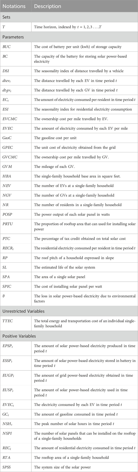
Table 1. Notations of the excel-based simulation model.

3.2.1.1 Total cost

Equation 3 represents the total annualized TTEC of a single-family household. It consists of the following costs: (1) the ownership cost of all GVs, (2) the cost of gasoline for GVs, (3) the ownership cost for EVs, (4); the cost of obtaining grid-powered electricity, and (5) the cost of generating solar-powered electricity. It is to be noted that the solar-powered electricity consists of solar system cost, battery cost, and the tax credit obtained from government. Since the total cost is annualized, the net cost of the solar system is spread over its estimated lifespan.

$\begin{array}{ll}\hfill TTEC=& {\displaystyle \sum _{t=1}^T}GVCMC\times NGV\times DSI\times {dtgv}_t+{\displaystyle \sum _{t=1}^T}GasC\times {GC}_t\hfill \\ \hfill & +{\displaystyle \sum _{t=1}^T}EVCMC\times NEV\times {DSI\times dtev}_t+{\displaystyle \sum _{t=1}^T}GPEC\times {EUGP}_t\hfill \\ \hfill & +{\displaystyle \sum _{t=1}^T}\left(\frac{SPIC\times SPSS+BUC\times BC-PTC\times \left[PIC\times SPSS+BUC\times BC\right]}{SL\times {EPSP}_t}\right)\hfill \end{array}(3)$

3.2.1.2 Residential electricity demand

Equation 4 represents the amount of residential electricity consumed by single-family households which depends on the energy usage per resident, the number of residents, and the seasonality factor.

${REC}_t={ESF}_t\times {EC}_t\times NR\forall t(4)$

3.2.1.3 EV electricity demand

Equation 5 suggests that the amount of electricity consumed by EVs in a single-family household depends on the number of EVs, EV electricity usage, and distance travelled by EV.

${EVEC}_t=NEV\times EVEC\times {DSI\times dtev}_t\forall t(5)$

3.2.1.4 Gasoline demand

Equation 6 indicates that the amount of gasoline consumed by GVs at a single-family household depends on the number of GVs, GV mileage, and distance travelled by GV.

${GC}_t=NGV\times \frac{{DSI\times dtgv}_t}{GVM}\forall t(6)$

3.2.1.5 Solar-powered electricity

Equation 7 allows to determine the rooftop area for a single-family household. The rooftop area depends on the household depends on the household base area and the roof pitch.

$RTA=\frac{HBA}{\cos \left({\tan }^{-1}RP\times 100\%\right)}(7)$

Equation 8 indicates that the number of solar panels that can be put on the rooftop depends on the rooftop area and proportion of rooftop area that can be used for solar panel installation.

$NSPI\times SPA\le PRTU\times RTA(8)$

Equation 9 suggests that the amount of solar power-based electricity produced depends on the number of peak solar hours, number of solar panels installed, power output of each solar panel, and loss in electricity due to environmental factors.

${EPSP}_t=\left(1-\vartheta \right)\times POSP\times NSPI\times {NSH}_t\forall t(9)$

Equation 10 is an electricity balance equation that states the total solar power-generated electricity in the current period, combined with the electricity stored in the battery from the previous period, must equal the sum of the solar power-based electricity consumed in the current period and the electricity stored in the battery.

${EPSP}_t+{ESSP}_{t-1}={EUSP}_t+{ESSP}_t\forall t(10)$

Equation 11 constrains the amount of solar power-based electricity stored in the battery is less than battery capacity.

${ESSP}_t\le BC(11)$

Equation 12 is a measure that estimates the solar system size in watts. The solar system size depends on the power output of each solar panel and the number of solar panels installed on the rooftop.

$SPSS=POSP\times NSPI(12)$

3.2.1.6 Adding grid power-based electricity to solar-powered electricity

Equation 13 ensures that the amount of solar power and grid power electricity supplied is equal to the residential and EV electricity demand.

${EUSP}_t+{EUGP}_t={REC}_t+{EVEC}_t\forall t(13)$

3.2.2 Second stage: Simulation runs and synthetic data development

The second stage of the three-stage evaluation framework involves developing synthetic data that can be used by the supervised machine learning models. To develop synthetic data, the energy balance simulation model (Equations 3–13) is run $N$ times, with each run indexed as $n=1,2,..N$ with varying parameters to estimate the TTEC for several single-family households. The parameters that were varied include: (1) number of residents, (2) house size, (3) number of EVs, (4) EV ownership cost, (5) EV efficiency, (6) Number of GVs, (7) GV ownership cost, (8) GV efficiency, (9) Solar implemented or not, (10) solar system size, (11) battery storage capacity, and (12) peak solar hours. Consequently, for a SML model, the TTEC parameter of the synthetic data becomes the dependent or response variable and the twelve parameters that are varied becomes the independent or predictor variables. Once synthetic data is generated, data cleaning and initial exploratory data analysis (EDA) is performed to understand the distribution of each parameter.

3.2.3 Supervised machine learning (SML) models

Once the synthetic data is cleaned and initial EDA is performed, numerous SML models are trained by splitting the data into training and testing data. The SML models that are trained and tested in this study are: (1) Linear Regression, (2) Ridge Regression, (3) Lasso Regression, (4) Decision Tree, (5) Bagging, (6) Random Forest, (7) Adaptive Boosting, and (8) Gradient Boosting. To select the best SML model, the performance metrics that are considered are: (1) Root Mean Square Error (RMSE), (2) Mean Absolute Percentage Error (MAPE), and (3) Adjusted R-squared.

4 Results

This section presents the results of the study. Section 4.1 presents the results of the first stage energy balance simulation model including sensitivity analysis for model validation. Section 4.2 presents the initial Exploratory Data Analysis (EDA) of second stage synthetic data, which is developed by running the energy balance simulation model several times by varying several input parameters. Section 4.3 presents the results of the third stage SML models.

4.1 First stage: energy balance simulation model results

This section presents the results of the first stage energy balance simulation model for individual households. In addition, we perform sensitivity analysis on few important parameters to validate the model, i.e., the model is providing insights as intended. These insights are cross validated with the literature as well as trials by multiple experts in this field of study. In this initial first stage study, we begin our analysis by examining a single-family household consisting of two residents, with a base area of 1781 square feet and two vehicles. The study focuses on comparing the TTEC performance of a single-family household by considering the system boundary configurations shown in Table 2. It is to be noted that, based on the configuration under consideration, the household utilizes a solar system size that fulfills the entire single-family household’s electricity demand. For example, in SE + GV, we consider a solar system size that fulfills residential electricity requirement, whereas in SE + EV, we consider a solar system size that fulfills both residential and EV charging electricity needs.

Table 2

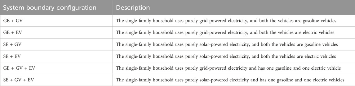
Table 2. System boundary configuration.

4.1.1 Comparing TTEC for different system boundary configurations

This section presents TTEC comparison for different system boundary configurations. In this study, the energy balance simulation model is run thirty times for each configuration to establish a confidence level for TTEC. Figure 3 shows the boxplots of the simulation runs which depicts the TTEC comparison of different system boundary configurations. It indicates that there is significant difference in TTEC for different system boundary configurations. Consistent with the results of Kassem et al. (2023) and Liang et al. (2022), the total cost of ownership for EVs when used in combination with SE is best. However, the total cost of ownership for GVs when used in combination with SE is worst, indicating that installing solar to meet only residential electricity needs can be an expensive value proposition. Consistent with the results of Coffman et al. (2017), we further observe that EVs are less expensive compared to GVs irrespective of the electricity source used indicating that the total cost of ownership for purely EVs are less compared to purely GVs. This is because numerous subsidies are provided by the government for EVs compared to GVs. In essence, different system boundary configurations for this specific single-family household can be ranked from least expensive to highest expensive as follows: (1) SE + EV, (2) SE + GV + EV, (3) GE + EV, (4) GE + GV + EV, (5) GE + GV, and (6) SE + GV. It is to be noted that this ranking is exclusively valid for this specific single-family household and may vary for single-family households that have different parameters. Figure 4 shows the cost split for each configuration, and it can be observed that the ownership cost for vehicles significantly contributes towards total cost compared to other costs. Here, the ownership cost includes all the costs except gasoline cost for GVs and electricity cost for EVs.

Figure 3

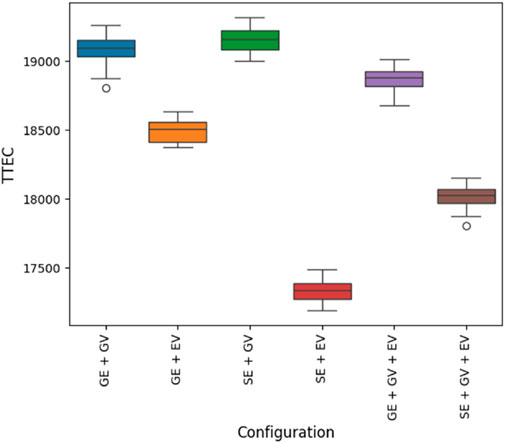
Figure 3. Cost comparison of different system boundary configurations.

Figure 4

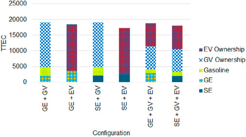
Figure 4. Cost components under different system boundary configurations.

4.1.2 The impact of solar system size on different configurations

In this section, we perform sensitivity analysis to validate the simulation model by varying the solar system size. Figures 5, 6 presents the TTEC performance and solar reliability analysis when solar system size is varied. They indicate that the TTEC for configurations decrease and then increase as solar system size is increased. The TTEC is least when all the electricity requirement for a household is met by SE. Furthermore, it is found that integrating SE with EV outperforms all the other configurations for wide range solar system size. However, breakeven points are observed for SE + GV and SE + GV + EV where TTEC is less than certain configurations when solar system sizes are lower and higher when solar system sizes are higher. This indicates that larger solar system sizes can increase costs when used in combination of GV. This result is consistent with Salles-Mardones et al. (2022) which suggests that smaller solar systems provide higher economic benefits compared to larger solar systems.

Figure 5

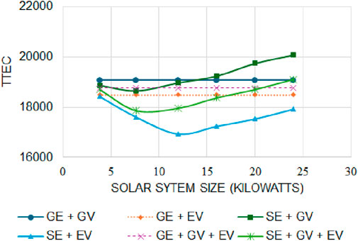
Figure 5. Cost comparison of different configurations when solar system size is varied.

Figure 6

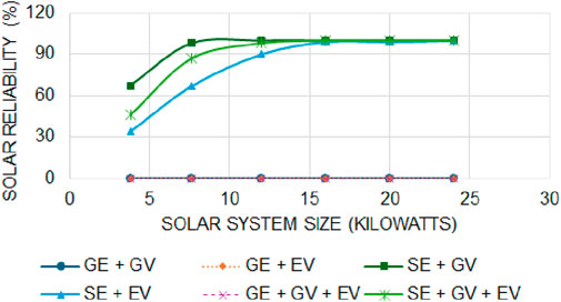
Figure 6. Solar system reliability under different configurations when solar system size is varied.

4.1.3 The impact of GV and EV mileage on different configurations

In this section, we further validate the energy balance simulation model by performing sensitivity analysis on GV and EV mileages. Figures 7, 8 present the results when GV and EV mileages are varied. They indicate that as mileage is increased, the TTEC decreases. In Figure 7, it can be observed that SE + GV + EV outperforms SE + EV for higher GV mileage indicating that a single-family household having solar system, EV and hybrid vehicles (typically, GVs with higher mileage are hybrid) are better than solar integration with EV, which is consistent with the results of Mitropoulos et al. (2017). In addition, it indicates that GV mileage significantly impacts TTEC. Figure 8 indicates that solar integration with EV has significantly lower TTEC compared to other configurations. In addition, the TTEC is stable for wide range of EV mileage indicating that the SE + EV adds stable value proposition to the owner. In both the Figures, break even points are observed where TTEC is higher at lower mileages and lower at higher mileages for certain configurations, which is consistent with the performed by Mitropoulos et al. (2017).

Figure 7

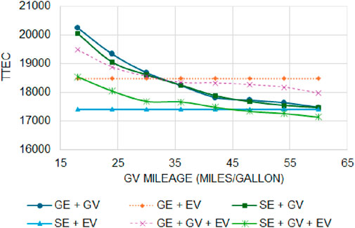
Figure 7. The impact of GV mileage on different configurations.

Figure 8

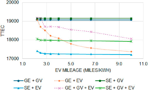
Figure 8. The impact of EV mileage on different configurations.

In summary, consistent with the results of the literature, we observed that even though there is significant difference in different system boundary configurations with solar integration with EV being best, numerous parameters such as subsidies, solar system size, and vehicle mileage makes the results inconclusive. Consequently, we seek to the understand the TTEC under varying conditions for different single-family households with different parameters and seek to determine the important parameters that contribute significantly to TTEC prediction.

4.2 Second stage: simulation runs and synthetic data analysis

In this second stage, the energy balance simulation model is run five hundred and fifty times to generate synthetic data that can be used to train the SML models in third stage. During this second stage, we estimate the TTEC for each run by varying the following parameters in the energy balance simulation model: (1) number of residents, (2) house size, (3) number of EVs, (4) EV ownership cost, (5) EV efficiency, (6) number of GVs, (7) GV ownership cost, (8) GV efficiency, (9) solar implemented or not, (10) solar system size, (11) battery storage capacity, and (12) peak solar hours. Therefore, we obtain synthetic data consisting of five hundred and fifty records and thirteen parameters (TTEC is also a parameter in synthetic data). Once synthetic data is developed, we perform initial Exploratory Data Analysis (EDA) to understand the distribution of various parameters. Figure 9 presents the results of the initial EDA performed on the synthetic data. It illustrates the following:

• The number of residents ranges between one to six with a median of three residents per household.

• Majority of households seem to have one EV.

• Majority of households have either one or two GVs.

• Majority of households do not have a solar system implemented.

• The house size seems to be normally distributed with a range between 1,000 and 3,500 square feet.

• GV Ownership and EV ownership cost seem to be uniformly distributed with a median of 0.57 and 0.52 per mile respectively.

• GV efficiency seems to be normally distributed with a mean of 40 miles per gallon. However, EV efficiency seems to be right skewed with a median of 3.12 miles per kwh.

• Solar system size and solar battery capacity are right skewed as majority of the households do not have solar system implemented.

• Peak solar hours seem to be normally distributed with two modes with peak solar hours ranging between 3.50–6.01 h per day

• The TTEC seems to be normally distributed with multiple modes. The total cost ranges between $6,512 - $38344. The median of TTEC of $19784 and mean of TTEC is $21211 indicating that there is a slight right skewness in the TTEC distribution.

Figure 9

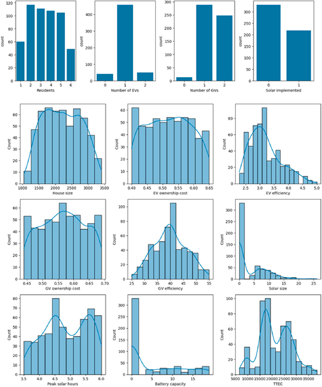
Figure 9. Initial EDA results performed on the synthetic data.

4.3 Results of supervised machine learning (SML) models

In the synthetic data, twelve parameters that include number of residents, house size, number of EVs, EV ownership cost, EV efficiency, Number of GVs, GV ownership cost, GV efficiency, solar implemented or not, solar system capacity, battery storage capacity, and peak solar hours become the independent variables or predictors for SML models. Moreover, TTEC becomes the dependent or response variable for SML models. To build SML models, we split the synthetic dataset into training and testing datasets. We split the data into 80–20, where 80% (440 out of 550) of the data is used for training the SML models and 20% (110 out of 550) of the data is used for testing the SML models. As discussed earlier in Section 3.2.3, we train eight different SML models that include: (1) Linear Regression, (2) Ridge Regression, (3) Lasso Regression, (4) Decision Tree, (5) Bagging, (6) Random Forest, (7) Adaptive Boosting, and (8) Gradient Boosting. In addition, to select the best SML model, the performance metrics that are used are: (1) Root Mean Square Error (RMSE), (2) Mean Absolute Percentage Error (MAPE), and (3) Adjusted R-squared. Table 3 presents the training and testing performance for different SML models. At first glance, it can be observed that all the SML models studied are able to predict the TTEC for single-family households with accuracy of more than 90% on testing dataset. This indicates that any of the SML models can be used and is good enough for predicting TTEC. However, comparing RMSE between training and testing datasets for different SML models indicate that Decision Tree, Bagging, Random Forest, Adaptive Boosting, and Gradient Boosting are overfitting models as the gap between RMSE on training and testing datasets is significantly high. This indicates that these SML models will predict with higher errors and lower accuracy on new datasets. In terms of the best SML model, regression models that include Linear Regression, Ridge Regression, and Lasso regression seem to be the best SML models as the difference in RMSE, MAPE, and Adjusted R-squared values between training and testing dataset is least. In addition, as RMSE and MAPE values are least and adjusted R-squared is highest, the regression SML models will have lower prediction errors and higher accuracy on new datasets. Therefore, any of the three SML regression models can be used in the real world to estimate the TTEC for single-family households rather than simulation model. Therefore, the SML regression models can be used as substitute for simulation model. This will reduce the computational complexity and allow the regression models to train themselves as new household’s TTEC are estimated and actual total costs are realized.

Table 3

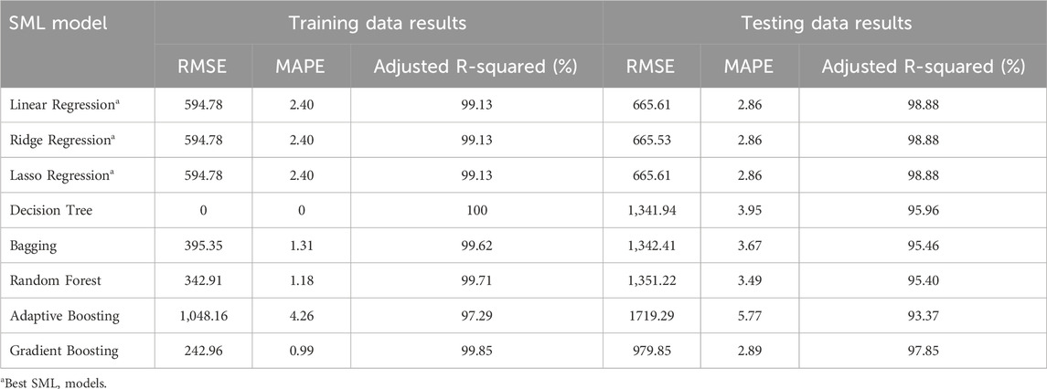
Table 3. Performance of different SML models.

Since, Regression SML models are best, we perform sequential forward selection of parameters, which is shown in Figure 10. It indicates that out of twelve parameters considered, six parameters are the most important parameters as there is marginal change in R-squared adjusted as the number of parameters are added after six. Chronologically, the parameters that are most important are: (1) House size, (2) Number of GVs, (3) Number of EVs, (4) GV ownership cost, (5) EV ownership cost, and (6) Solar implemented. Figure 11 presents the EDA for important parameters selected by SML regression models. It clearly shows strong correlation between these parameters and TTEC. In addition, it can be observed that as we move from most important to least important parameter, the significance of the relationship between the TTEC and the parameter seems to decrease. For instance, house size significantly impacts the total price compared to having solar implemented or not. Furthermore, a positive correlation between TTEC and all the parameters except solar implemented is observed indicating that as parameter value increases, TTEC also increases. However, if solar is implemented, TTEC decreases. The results of the study also provide counter intuitive notion, i.e., the number of residents, GV and EV mileage, Solar system size, battery capacity and peak solar hours are not significant parameters and marginally contribute to the TTEC prediction.

Figure 10

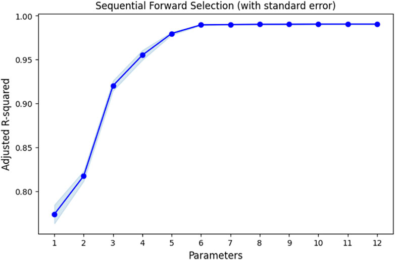
Figure 10. Sequential Forward Selection for best SML regression models.

Figure 11

Figure 11. EDA for important parameters selected by best SML regression models.

5 Conclusion

This paper focuses on predicting the total transportation and energy costs (TTEC) for single-family households. A system boundary consisting of grid-powered electricity (GE) and solar-powered electricity (SE) as energy inputs and gasoline vehicles (GVs) and electric vehicles (EVs) as transportation methods for energy outputs is considered. A novel three stage prediction framework is developed that aims to predict the TTEC for any given single-family household with specific set of parameters and determine the important parameters that contribute towards predicting TTEC. The first stage of the prediction framework involves developing energy balance simulation model for an individual household. The second stage of the prediction framework involves running the simulation model several times to develop synthetic data. In the third stage, several supervised machine learning (SML) models are trained and tested by using the synthetic data to determine the best SML model as well as important parameters that contribute significantly towards predicting TTEC. A case study of single-family households in Central Texas region is used as an application of the prediction framework. The results of the first stage energy balance simulation model indicate that there is a significant difference in TTEC for different system boundary configurations for a single-family household. In fact, it is found that SE integration with EVs is the best and SE integration with GVs being the worst in terms of reducing costs. Currently, the subsidies provided to both solar systems and EVs favor solar and EV integration. However, this notion of solar and EV integration being best is still ambiguous and questionable as other factors impact their performance. For example, a household having both GV and EV along with solar system seems to outperform solar and only EV integration when the GV is hybrid given their high mileage.

In the second stage, the simulation model is run five hundred and fifty times, and the initial EDA indicates that the total cost ranges between $6,537-$38344 with a mean of $21211. In third stage, eight different SML models are trained and tested that include: (1) Linear Regression, (2) Ridge Regression, (3) Lasso Regression, (4) Decision Tree, (5) Bagging, (6) Random Forest, (7) Adaptive Boosting, and (8) Gradient Boosting. The performance metrics that are used to evaluate the SML models are: (1) Root Mean Square Error (RMSE), (2) Mean Absolute Percentage Error (MAPE), and (3) Adjusted R-squared. The results of the third stage indicate that regression SML models are best in predicting the total costs with an adjusted R-squared of 99.13% and 98.88% on training and testing datasets, respectively. In addition, the parameter analysis of regression SML models suggests that the house size, number of GVs, number of EVs, EV and GV ownership costs, and implementation of solar at households are the most important parameters that contribute significantly towards predicting the TTEC of a single-family household. Counterintuitively, number of residents, GV and EV mileage, Solar system size, battery capacity and peak solar hours are not significant parameters and marginally contribute to the TTEC prediction. In summary, since the best SML regression model is trained and tested with the energy balance simulation model synthetic data, the SML regression model can be used as a substitute for simulation model, thereby avoiding the computational burden of running simulation model for each new single-family household.

Even though the SML regression models predict with high degree of accuracy, the study has several limitations. First, the sample size of the synthetic data can be increased. Second, the study fails to consider variability in numerous other parameters such as variability in prices of gasoline and electricity as well as variability in distances travelled by households. In addition, different models can be developed for with and with solar to study whether parameters such as solar system size, battery capacity, roof pitch, and peak solar hours impact the SML model performance. Therefore, future research will include expanding the study to fill these gaps.

Data availability statement

The original contributions presented in the study are included in the article/Supplementary Material, further inquiries can be directed to the corresponding author.

Author contributions

VG: Conceptualization, Data curation, Formal Analysis, Investigation, Methodology, Validation, Writing–original draft, Writing–review and editing. AO: Formal Analysis, Investigation, Methodology, Software, Validation, Writing–review and editing. RS: Conceptualization, Formal Analysis, Investigation, Methodology, Validation, Writing–original draft, Writing–review and editing.

Funding

The author(s) declare that no financial support was received for the research, authorship, and/or publication of this article.

Conflict of interest

The authors declare that the research was conducted in the absence of any commercial or financial relationships that could be construed as a potential conflict of interest.

Generative AI statement

The author(s) declare that no Generative AI was used in the creation of this manuscript.

Publisher’s note

All claims expressed in this article are solely those of the authors and do not necessarily represent those of their affiliated organizations, or those of the publisher, the editors and the reviewers. Any product that may be evaluated in this article, or claim that may be made by its manufacturer, is not guaranteed or endorsed by the publisher.

Supplementary material

The Supplementary Material for this article can be found online at: https://www.frontiersin.org/articles/10.3389/fenef.2024.1502854/full#supplementary-material

References

Aggarwal, V., and Walker, E. (2024). How much energy does a solar panel produce?. Available at: https://www.energysage.com/solar/solar-panel-output/.

Google Scholar

Ajanovic, A. (2015). The future of electric vehicles: prospects and impediments. WIREs Energy Environ. 4 (6), 521–536. doi:10.1002/wene.160

CrossRef Full Text | Google Scholar

Allen, N., and Tynan, C. (2024). Solar panel size and weight: a comprehensive guide. Available at: https://www.forbes.com/home-improvement/solar/solar-panel-size-weight-guide/#:∼:text=More%20See%20Less-,60%20Cells,of%20frames%20and%20mounting%20equipment.

Google Scholar

Betterton, R., Subitch, R., and Brock, T. (2024). Average cost of car maintenance: 2024 estimates. Available at: https://www.bankrate.com/loans/auto-loans/average-car-maintenance-costs/.

Google Scholar

Boström, T., Babar, B., Hansen, J. B., and Good, C. (2021). The pure PV-EV energy system–A conceptual study of a nationwide energy system based solely on photovoltaics and electric vehicles. Smart Energy 1, 100001. doi:10.1016/j.segy.2021.100001

CrossRef Full Text | Google Scholar

Cieslik, W., Szwajca, F., Golimowski, W., and Berger, A. (2021). Experimental analysis of residential photovoltaic (PV) and electric vehicle (EV) systems in terms of annual energy utilization. Energies 14 (4), 1085. doi:10.3390/en14041085

CrossRef Full Text | Google Scholar

Coffman, M., Bernstein, P., and Wee, S. (2017). Integrating electric vehicles and residential solar PV. Transp. Policy 53, 30–38. doi:10.1016/j.tranpol.2016.08.008

CrossRef Full Text | Google Scholar

Danielis, R., Giansoldati, M., and Rotaris, L. (2018). A probabilistic total cost of ownership model to evaluate the current and future prospects of electric cars uptake in Italy. Energy Policy 119, 268–281. doi:10.1016/j.enpol.2018.04.024

CrossRef Full Text | Google Scholar

Fachrizal, R., and Munkhammar, J. (2020). Improved photovoltaic self-consumption in residential buildings with distributed and centralized smart charging of electric vehicles. Energies 13 (5), 1153. doi:10.3390/en13051153

CrossRef Full Text | Google Scholar

Falahi, M., Chou, H. M., Ehsani, M., Xie, L., and Butler-Purry, K. L. (2013). Potential power quality benefits of electric vehicles. IEEE Trans. Sustain. energy 4 (4), 1016–1023. doi:10.1109/tste.2013.2263848

CrossRef Full Text | Google Scholar

Fields, S., Walker, E., and Langone, A. (2024). Solar battery cost: why they're not always worth it. Available at: https://www.energysage.com/energy-storage/how-much-do-batteries-cost/.

Google Scholar

Fitzpatrick, A., and Jordan, J. R. (2024). Axios houston. Available at: https://www.axios.com/local/houston/2024/06/25/car-miles-driven-texas-walk-score.

Google Scholar

Göhler, G., Klingler, A. L., Klausmann, F., and Spath, D. (2021). Integrated modelling of decentralised energy supply in combination with electric vehicle charging in a real-life case study. Energies 14 (21), 6874. doi:10.3390/en14216874

CrossRef Full Text | Google Scholar

Gonela, V., Altman, B., Zhang, J., Ochoa, E., Murphy, W., and Salazar, D. (2020). Decentralized rainwater harvesting program for rural cities considering tax incentive schemes under stakeholder interests and purchasing power restrictions. J. Clean. Prod. 252, 119843. doi:10.1016/j.jclepro.2019.119843

CrossRef Full Text | Google Scholar

Hassan, Q., Viktor, P., J Al-Musawi, T., Mahmood Ali, B., Algburi, S., Alzoubi, H. M., et al. (2024). The renewable energy role in the global energy Transformations. Renew. Energy Focus 48, 100545. doi:10.1016/j.ref.2024.100545

CrossRef Full Text | Google Scholar

IEA (2024). Global EV outlook 2024. Paris: IEA. Available at: https://www.iea.org/reports/global-ev-outlook-2024.

Google Scholar

Jones, B., Nguyen-Tien, V., and Elliott, R. J. (2023). The electric vehicle revolution: critical material supply chains, trade and development. World Econ. 46 (1), 2–26. doi:10.1111/twec.13345

CrossRef Full Text | Google Scholar

Kassem, Y., Gokcekus, H., and Aljatlawe, A. (2023). Utilization of solar energy for electric vehicle charging and the energy consumption of residential buildings in northern Cyprus: a case study. Eng. Technol. and Appl. Sci. Res. 13 (5), 11598–11607. doi:10.48084/etasr.6142

CrossRef Full Text | Google Scholar

Liang, J., Qiu, Y. L., and Xing, B. (2022). Impacts of the co-adoption of electric vehicles and solar panel systems: empirical evidence of changes in electricity demand and consumer behaviors from household smart meter data. Energy Econ. 112, 106170. doi:10.1016/j.eneco.2022.106170

CrossRef Full Text | Google Scholar

Liu, Z., Song, J., Kubal, J., Susarla, N., Knehr, K. W., Islam, E., et al. (2021). Comparing total cost of ownership of battery electric vehicles and internal combustion engine vehicles. Energy Policy 158, 112564. doi:10.1016/j.enpol.2021.112564

CrossRef Full Text | Google Scholar

Martin, H., Buffat, R., Bucher, D., Hamper, J., and Raubal, M. (2022). Using rooftop photovoltaic generation to cover individual electric vehicle demand—a detailed case study. Renew. Sustain. energy Rev. 157, 111969. doi:10.1016/j.rser.2021.111969

CrossRef Full Text | Google Scholar

Mitropoulos, L. K., Prevedouros, P. D., and Kopelias, P. (2017). Total cost of ownership and externalities of conventional, hybrid and electric vehicle. Transp. Res. procedia 24, 267–274. doi:10.1016/j.trpro.2017.05.117

CrossRef Full Text | Google Scholar

Petroleum and Other Liquids (2024). Petroleum and other liquids. U.S. Energy Information Administration. Available at: https://www.eia.gov/dnav/pet/hist/LeafHandler.ashx?n=pet&s=emm_epm0u_pte_stx_dpg&f=m.

Google Scholar

Raman, M., Darcy, M., Czernia, D., and Bowater, J. (2024). Solar panel calculator. Available at: https://www.omnicalculator.com/ecology/solar-panel.

Google Scholar

Residential Average Monthly kWh and Bills (2024). Residential average monthly kWh and Bills. Available at: https://data.austintexas.gov/widgets/d9pb-3vh7?mobile_redirect=true.

Google Scholar

Residential Clean Energy Credit (2024). Residential clean energy credit. Available at: https://www.irs.gov/credits-deductions/residential-clean-energy-credit.

Google Scholar

Roof pitch angle and slope factor chart (2024). Roof pitch angle and slope factor chart. Available at: https://www.riversidesheetmetal.net/metal-roofing/roof-pitch/.

Google Scholar

Salles-Mardones, J., Flores-Maradiaga, A., and Ahmed, M. A. (2022). Feasibility assessment of photovoltaic systems to save energy consumption in residential houses with electric vehicles in Chile. Sustainability 14 (9), 5377. doi:10.3390/su14095377

CrossRef Full Text | Google Scholar

Solar Panel Cost (2024). Solar panel cost. Available at: https://www.solar.com/learn/solar-panel-cost/#calc.

Google Scholar

United States Environmental Protection Agency (2022). EPA report: U.S. Cars achieve record high fuel economy and low emission levels as companies fully comply with standards. Available at: https://www.epa.gov/newsreleases/epa-report-us-cars-achieve-record-high-fuel-economy-and-low-emission-levels-companies.

Google Scholar

US Monthly Total Vehicle Miles Traveled (2024). US monthly total vehicle miles traveled. Available at: https://ycharts.com/indicators/us_monthly_total_vehicle_miles_traveled.

Google Scholar

Walker, E., and McDevitt, C. (2024). How long do solar panels last? Available at: https://www.energysage.com/solar/how-long-do-solar-panels-last/.

Google Scholar

Weldon, P., Morrissey, P., and O’Mahony, M. (2018). Long-term cost of ownership comparative analysis between electric vehicles and internal combustion engine vehicles. Sustain. Cities Soc. 39, 578–591. doi:10.1016/j.scs.2018.02.024

CrossRef Full Text | Google Scholar

Wu, G., Inderbitzin, A., and Bening, C. (2015). Total cost of ownership of electric vehicles compared to conventional vehicles: a probabilistic analysis and projection across market segments. Energy policy 80, 196–214. doi:10.1016/j.enpol.2015.02.004

CrossRef Full Text | Google Scholar

Zargary, S. (2023). How much electricity does an electric car use?. Available at: https://www.gencellenergy.com/resources/blog/ev-charging-power-car-electricity-usage/.

Google Scholar