 Ali Pourzangbar
 Mahdi Jalali3
- 1Institute for Water and River Basin Management—Hydraulic Engineering and Water Resources Management, Karlsruher Institut für Technologie (KIT), Karlsruhe, Germany
- 2Department of Civil and Building Engineering and Architecture, Università Politecnica delle Marche, Ancona, Italy
- 3Department of Civil Engineering, Tehran University, Tehran, Iran
This study provides an extensive review of over 200 journal papers focusing on Machine Learning (ML) algorithms’ use for promoting a sustainable management of the marine and coastal environments. The research covers various facets of ML algorithms, including data preprocessing and handling, modeling algorithms for distinct phenomena, model evaluation, and use of dynamic and integrated models. Given that machine learning modeling relies on experience or trial-and-error, examining previous applications in marine and coastal modeling is proven to be beneficial. The performance of different ML methods used to predict wave heights was analyzed to ascertain which method was superior with various datasets. The analysis of these papers revealed that properly developed ML methods could successfully be applied to multiple aspects. Areas of application include data collection and analysis, pollutant and sediment transport, image processing and deep learning, and identification of potential regions for aquaculture and wave energy activities. Additionally, ML methods aid in structural design and optimization and in the prediction and classification of oceanographic parameters. However, despite their potential advantages, dynamic and integrated ML models remain underutilized in marine projects. This research provides insights into ML’s application and invites future investigations to exploit ML’s untapped potential in marine and coastal sustainability.
1 Introduction
Coastal areas are of vital significance due to their crucial role in supporting aspects such as biodiversity, economic activity, cultural heritage, climate regulation, food security, recreational opportunities, and strategic importance (Neumann et al., 2017). Ensuring their sustainability, however, is a challenge that requires addressing various factors, among which, climate change adaptation, beach protection and water quality management. One approach to ensuring the sustainability of coastal areas involves conducting a thorough examination of each contributing factor by employing data analysis and suitable methods. Effective data analysis and augmentation is, therefore, essential for informed decision-making and sustainable management of coastal areas.
The amount of data related to coastal systems has dramatically increased recently (Goldstein et al., 2019). This data, which often covers large areas and spans long periods of time, is now available in high resolution and can be accessed quickly. This has led to more opportunities for research on the sustainability of activities evolving in coastal areas. However, handling large and complex datasets, as well as identifying their patterns and trends, is not a convenient task. Despite their widespread use and mathematical rigor, conventional statistical techniques, including descriptive statistics (Emmanouil et al., 2020), inferential statistics (Agarwal and Manuel, 2008), regression analysis (Davidson et al., 1996; Hall et al., 2002), correlation analysis (Szmytkiewicz et al., 2000; Kroon et al., 2008; Ruiz de Alegría-Arzaburu et al., 2010), Analysis of Variance (ANOVA) (Martins et al., 2010), and Principal Component Analysis (PCA) (Hua et al., 2007; Miller and Dean, 2007), have limitations when processing large and complex data sets, and can present challenges in terms of interpretability. This has prompted researchers to explore alternative, more sophisticated approaches such as ML, which enables researchers to draw insights from data in a more efficient, accurate and automated way.
ML is a rapidly growing field that has the potential to make significant contributions to the sustainable use and management of marine and coastal environments. This by helping to better understand and predict the impacts of human activities and natural phenomena on coastal ecosystems and identify potential threats. The link between using machine learning to simulate coastal and marine events and sustainability revolves around creating models and taking action. Machine learning employs large amounts of data to create simulations for different scenarios, such as wave propagation or water quality management. These simulations help us fine-tune our actions, like improving wave energy converters or changing shipping paths to avoid pollution. Moreover, these simulations can guide our work towards adapting and mitigating the effects of environmental changes, like coastal erosion caused by rising sea levels. In essence, machine learning offers crucial insights that contribute to improved, sustainable care of our coastal and marine environments.
Typically, the primary input of ML algorithms consists of a data set in various forms such as numeric, image, DEMs collected by Lidar (light detection and ranging), video, and geographic information systems (GIS) data, which are mapped and visualized using GIS. The main output of ML algorithms in coastal engineering can vary depending on the specific application and dataset being used, which includes prediction [e.g., coastal flooding risk (Park and Lee, 2020), storm surge (Sajjad et al., 2020), wave height (Dogan et al., 2021), sediment transport (Pourzangbar et al., 2017b; 2017c; 2017a) and beach erosion (Beuzen et al., 2019)], image processing using satellite imagery data (Agrafiotis et al., 2019) or drone footage (Provost et al., 2020), pattern recognition [e.g., patterns of sediment transport (Liu et al., 2021)], placement optimisation (Cuadra et al., 2016; Sarkar et al., 2016; Neshat et al., 2019), optimization by identifying the most efficient and cost-effective solutions for protecting the coast from erosion and flooding, monitoring (e.g., using sensor data to detect erosion or changes in water quality), anomaly detection (e.g., unusual changes in water quality), and decision making (Lazuardi et al., 2021) by providing decision support to coastal managers and engineers. However, the applicability of ML approaches in coastal engineering is influenced by various factors such as data quality, computational resources, the complexity of the coastal system, and the choice of appropriate algorithms.
Several ML methods have been used to study the sustainable use of coastal areas, including: Artificial Neural Networks (ANNs) used for predictions such as water quality (Chen and Ma, 2010), river classification based on the water quality index (Wong et al., 2021), wave height (Rao and Mandal, 2005; Günaydin, 2008) and beach erosion (Hashemi et al., 2010) and tidal prediction; Decision Trees (DTs) used for classifying the dominating environmental factors; Random Forests (RFs) used for regression and classification tasks, such as predicting the effect of human activities on the coastal environment and water quality index modelling (Sakaa et al., 2022); Support Vector Machines (SVMs) used for solving classification and regression problems, such as identifying the most vulnerable areas in coastal zones; K-Nearest Neighbors (KNN) used for clustering and classification tasks, such as grouping coastal regions based on their sustainability indicators; Ensemble Methods used for improving the accuracy of predictions and classifications, such as predicting the impact of climate change on sustainability of coastal activities, among others.
ML has been widely used in numerous research studies, but there still exists a knowledge gap regarding the selection of parameters, choice of predictive models (be they dynamic or static), domain adaptation, and use of integrated models for analyzing complex systems and evaluating the effects of multiple factors. In relation to data treatment, many existing works have relied on simple heuristic methods or rules of thumb; however, there are more solid mathematical and metaheuristic methods for data preprocessing and parameter identification, highlighted in this paper. Choosing the correct model can be challenging and there is not a definitive method to identify the most suitable ML model for a given problem. In general, the ML approach used to solve a specific issue is selected through a process of trial and error. However, comparing how models perform under different conditions can aid in selecting the most suitable one for a specific issue. To the best of authors’ knowledge, there is not one single paper that offers comprehensive information about the data preprocessing and preparation phase. This paper provides an extensive review of various methodologies employed in coastal engineering to handle datasets. The main focus of this paper is to understand how ML models contribute to the sustainable use and management of marine and coastal environments, rather than the technical intricacies of their setup. The primary goal is to provide a critical review of literature that utilized ML approaches to manage marine phenomena. This review sheds some light on how to prepare parameters and datasets for input into the ML model, the pros and cons of various models, the suitability of ML methods for certain conditions, and their shortcomings and deficiencies.
Although numerous papers have discussed modeling coastal phenomena using experimental, numerical, and mathematical methodologies, the focus of the current paper is exclusively on literature that implemented ML techniques for modeling coastal and marine events. The selected literature spans a broad range of topics from data preprocessing and parameter considerations to different kinds of ML models used for various purposes. Due to the large amount of published papers, the focus of our contribution was directed towards resources published in reputable international journals such as Elsevier, Springer, IWA, Taylor and Francis, Wiley, ASCE, among others. The papers were chosen based on their publication in reputable international journals and were retrieved through online searches using relevant keywords. Among the publications, Coastal Engineering (Elsevier) with 18 papers and Ocean Engineering (Elsevier) with 17 papers, had the most papers in this area. The majority of the sources are fairly recent, predominantly within the past 10 years. Nevertheless, this paper includes some older references that established the groundwork for newer methods. Roughly, fewer than 5% of the literature we reviewed was published before 2000, about 14% between 2000 and 2010, 22% between 2010 and 2015, and over 60% in the last 10 years.
While ML has been implemented in numerous studies, knowledge gaps exist in areas such as parameter selection, choice of models for making predictions (dynamic or static), domain adaptation, and the use of integrated models for modeling complex systems. The emphasis of the paper is on the contribution of ML models to the sustainable use and management of the marine and coastal environment, rather than on the technical details of their configuration.
The paper is structured as follows: Section 2 discusses the key components of data analysis and preprocessing, including data collection and preparation for the modeling process. Section 3 focuses on studies that have applied AI to coastal engineering for sustainable outcomes. The paper also evaluates the accuracy and robustness of the different models in Section 4. Finally, the paper summarizes all the information presented and concludes with a list of references.
2 Data preparation (preprocessing)
Data preparation involves transforming raw data into a format that can be used by ML algorithms for extracting insights or predicting outcomes. This process is vital in ML as it considerably affects the performance of the model (Kelleher et al., 2015). In the event of missing or invalid data, the algorithm either cannot process it or yields less precise, possibly erroneous results. This procedure starts with the acquisition of raw data (refer to Section 2.2), followed by data integration, which entails consolidating data from various sources into a unified dataset. This is succeeded by data cleansing to rectify missing values and outliers (refer to Section 2.4), and then selecting the most pertinent features from the input parameters (feature selection or dimensionality reduction) (see Section 2.5). Subsequently, feature engineering is undertaken, which involves generating new variables from existing parameters using dimensional analysis (DA). Lastly, data transformation is carried out, which involves altering the scale or distribution of variables, such as through data normalization. Figure 1 depicts the multiple phases required for data preprocessing and the methods linked with each step. The upcoming sections provide a detailed explanation of these methods.
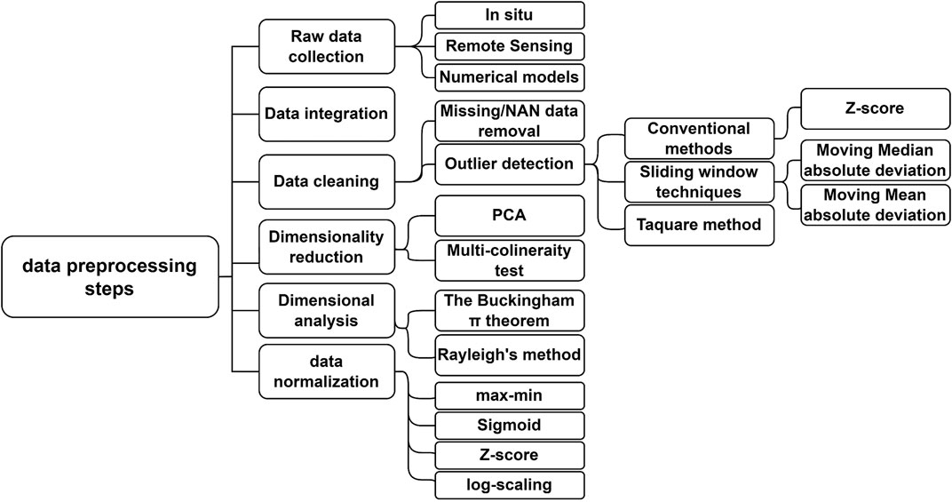
FIGURE 1. Data preprocessing steps and their corresponding necessary tasks that must be accomplished.
2.1 Marine data types
In coastal engineering, data can come in different forms (Huang et al., 2015) and can be classified into different types based on their identity, format, and structure. Some examples of coastal data types include:
(1) Numeric data (Timmermans et al., 2020), which includes measurements of various physical parameters such as water level, wave height, current velocity, sediment concentration. Such data are typically collected using instruments such as tide gauges, wave gauges, current meters, and sediment samplers. For example, time-series data such as ocean temperature records, sea level measurements, and storm surge data represented by a sequence of observations or measurements taken at regular intervals over time.
(2) Image data (Vos et al., 2019; Turner et al., 2021), which includes aerial and satellite imagery, as well as ground-based photographs. These data can be used to study coastal morphology, vegetation, and land use patterns.
(3) Point Cloud data (Gomez, 2022), represented by a set of 3D points that can be used to create 3D models of coastal terrain and structures. Point cloud data is often collected using light detection and ranging (LiDAR) systems and can be used to create high-resolution digital elevation models (DEMs) of coastal topography.
(4) Video data (Smit et al., 2007; Kim et al., 2020; Kim and Kim, 2020), which includes footage captured by cameras, this data can be used to observe the coastal dynamics and measure the beach profile, the shoreline position, and the wave breaking patterns.
(5) Text data (Brown et al., 2021), represented by written or spoken words, can be analyzed using natural language processing (NLP) techniques. Examples of text data in coastal engineering include social media posts, news articles, and scientific publications.
The following are the most well-known methods for collecting the data mentioned above: field observations, remote sensing measurements, experimental studies, numerical and mathematical models. Both the availability of equipment and the objective of the study influence the selection of the data collection medium (Prata et al., 2019).
2.2 Marine data resources
Data collection within the realm of marine sciences principally relies on three distinctive methods: in-situ observations, remote sensing techniques, and the use of mathematical and numerical models, as outlined by Verwega et al. (2021). In-situ data collection encompasses ship-based measurements, the deployment of moorings, gliders, autonomous underwater vehicles, drifters and floats, the use of sea-floor optic cables, and laboratory analyses. Field observations remain essential for the collection of real-world data on coastal processes, such as wave heights and tidal levels. In-situ instruments are highly accurate with proper maintenance but may have low-time frequency data for large areas. They offer historical climate trend insights not available from remote sensing and are less affected by atmospheric conditions. These observations serve to validate numerical models that simulate coastal processes and predict the behavior of the coastal system, including wave patterns, tidal currents, and shoreline evolution.
Remote sensing involves acquiring data on coastal topography, bathymetry, and other significant parameters through satellite and airborne platforms. Remote sensing technologies are divided into three categories: satellite, ground-based, and drones (Elsayed et al., 2021). The data thus collected enable the generation of high-resolution coastal environmental maps. Although satellites are powerful tools, they face limitations in obtaining high-resolution regional-scale imagery. Clouds can hinder data capture, and high-resolution imagery can be challenging to interpret (Elsayed et al., 2021). A combination of satellite- and ground-based remote sensing and drones could be effective in future marine engineering evaluations. Economically, combining these tools may be comparable to in-situ techniques in terms of overall cost. Such technology could enable rapid, high-resolution water condition assessments and enhance our understanding of water resource processes. Mathematical and numerical models generate data by simulating real-life systems or processes using mathematical equations and algorithms (Xie and Arkin, 1996). They provide the capability to extend observational data, even to the point of simulating future climate scenarios (Eyring et al., 2016). Nonetheless, it is crucial to understand that these models only approximate real-world scenarios and can encompass spatial and temporal scales that exceed the scope of observational data (Matthes et al., 2020). The outputs from these models are typically available on a unique grid, contingent on the specific simulation. For instance, climate models customarily provide a four-dimensional space-time grid. Consequently, the comparison of model outputs with measurements invariably necessitates interpolation or data aggregation. Table 1 provides a detailed summary of the advantages and disadvantages associated with these diverse data collection methodologies.
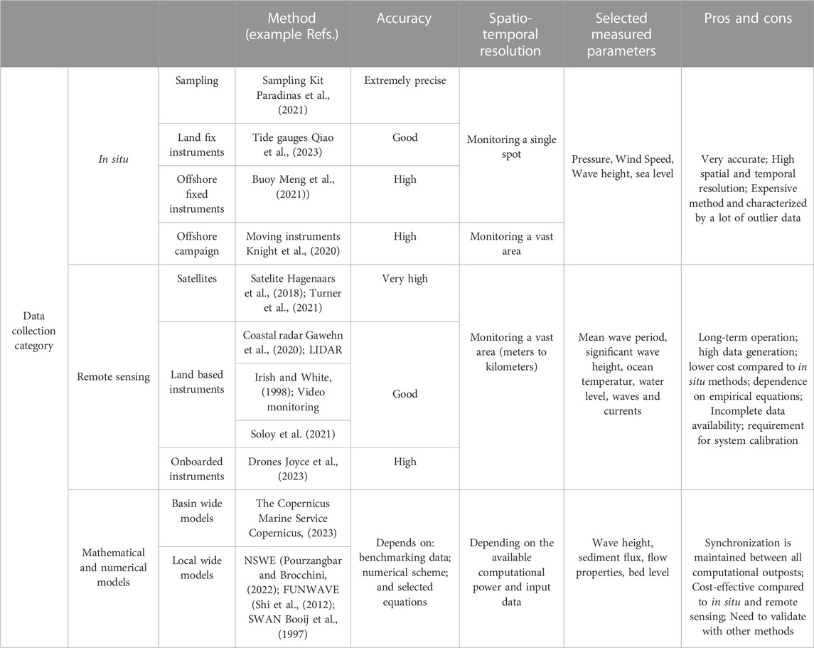
TABLE 1. Detailed information of the various data collection methods in coastal engineering.
2.3 Data cleaning: outlier detection
Several factors can influence the quality of observational data. These include inaccuracies in the instruments, malfunctions of the equipment, disruptions from external sources, mistakes during data conversion, communication mishaps, and significant unforeseen errors (Yu et al., 2022). Such anomalies can pose major threats to operational functionality, downstream operations, system resilience, and cleaner production (Ba-Alawi et al., 2021). Therefore, these should be detected promptly and their data rectified to ensure more realistic measurements.
Anomaly detection methods are generally categorized into various types (see Figure 2) such as Statistical Methods, that utilize the properties of the underlying data distribution to identify anomalies (Chandola et al., 2009); Distance-based Methods, which calculate the distance between data points and identify the outliers based on a certain distance threshold (Ramaswamy et al., 2000); Density-based Methods, which estimate the density of data points and identify outliers as those points that reside in low-density regions (Ester et al., 1996); Machine Learning-based Methods, which employ supervised, unsupervised, or semi-supervised ML algorithms to detect outliers (Pimentel et al., 2014); and Ensemble Methods, which combine multiple outlier detection algorithms to improve the overall performance (Zimek et al., 2012). The choice of method, or combination of methods for better results, depends on the nature of the data and the specific problem being addressed.
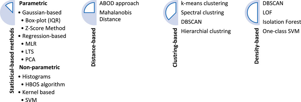
FIGURE 2. Various outlier detection appproaches.
Mahmoodi and Ghassemi (2018) used outlier detection algorithms to improve wave height predictions, while Oehmcke et al. (2015) demonstrated the effectiveness of ML for identifying significant events in marine long-term data. Daranda and Dzemyda (2020) developed a method combining the Density-Based Spatial Clustering of Applications with Noise (DBSCAN) clustering algorithm and k-nearest neighbors analysis for detecting marine traffic anomalies. These studies highlight the potential of leveraging advanced algorithms and ML in marine data analysis and decision-making. This section aims to provide a survey of contemporary outlier detection techniques, comparing their motivations, advantages, and disadvantages. Outliers can significantly impact the results, which makes addressing or eliminating them before analysis and model development crucial.
Considering the learning algorithm, three main methodologies exist for outlier detection (Hodge and Austin, 2004): 1) unsupervised approach, which uses a learning technique to identify outliers without prior knowledge of the data. The data is treated as a static distribution, and the most distant points are flagged as potential outliers; 2) supervised classification method, which requires pre-labeled data. It allows for online classification, where the classifier continuously learns the model and classifies new data as normal or abnormal, and finally 3) semi-supervised recognition technique, which only learns the normal class, using pre-classified data. It can distinguish new data as normal or novel based on its proximity to the boundary of normality. The choice of an outlier detection method depends on the data type, the number of vectors and attributes, speed and accuracy requirements, and the ability to accurately identify outliers. The key factors in choosing a method are selecting an algorithm that can handle the data and defining a suitable neighborhood for the outlier.
2.4 Dimensionality reduction
Incorporating parameters that are not relevant can result in intricate models that pose significant challenges in interpretation and execution compared to the models developed using the most crucial parameters (Pourzangbar, 2012). That is the reason why the focus is placed on building ML models using the most crucial parameters. These parameters are not only essential for the model’s output, but also are unconnected with other input parameters. To derive the most important dimensions (parameters) in the input space, there are several methods including min/max autocorrelation factor analysis (MAFA), dynamic factor analysis (DFA), Least Absolute Shrinkage and Selection Operator (LASSO), Independent Component Analysis (ICA), multicollinearity test and PCA. Table 2 summarizes some famous dimensionality reduction approaches used in marine engineering. The latter two methods are explained below.
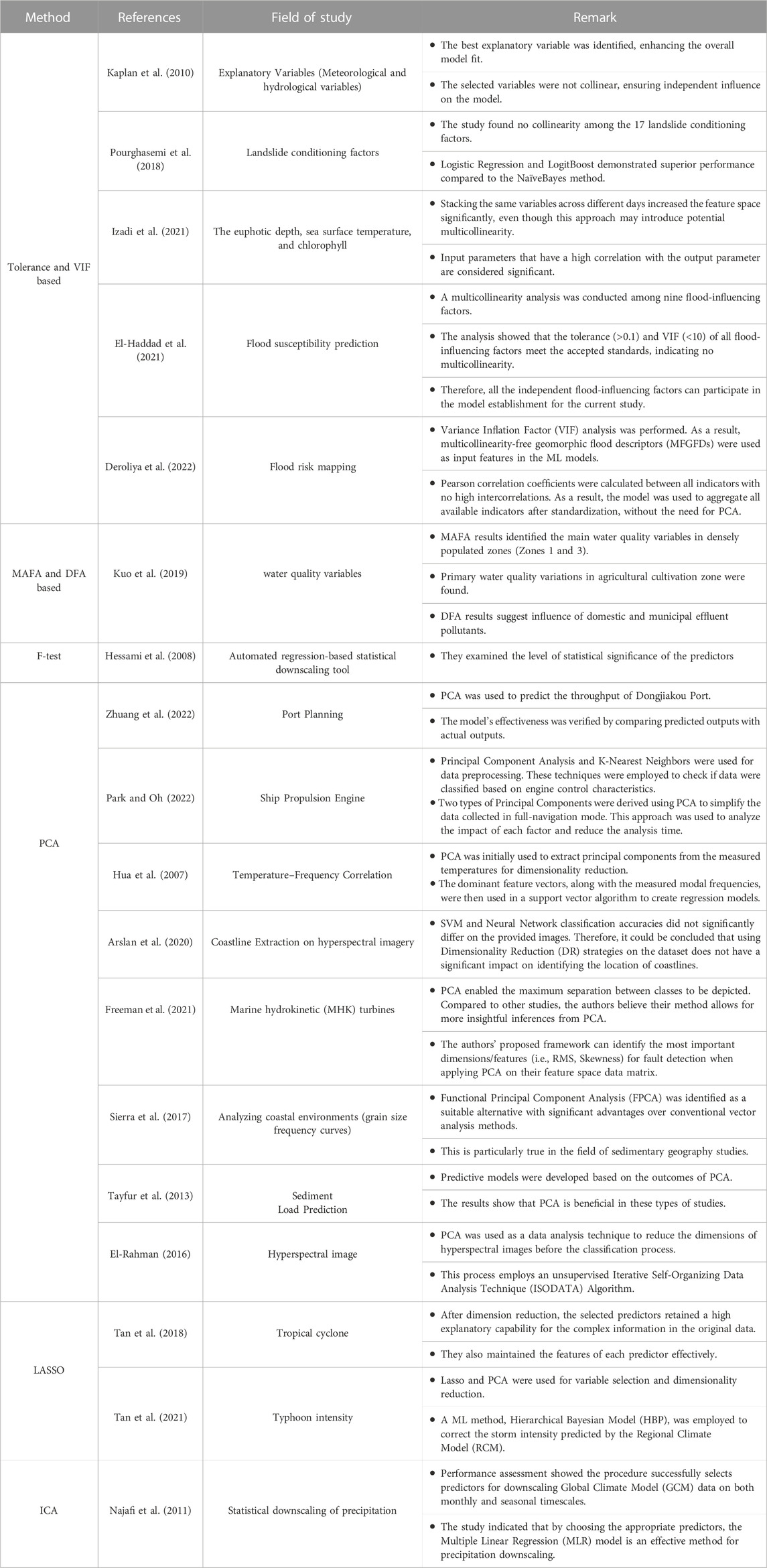
TABLE 2. Some well-known dimensionality reduction approaches and their example references.
2.4.1 Multicollinearity
Multicollinearity is a common issue that can arise in regression analysis when two or more predictor variables in a model are highly correlated with each other. This can cause problems in the analysis, such as unstable and unreliable coefficient estimates. There are several methods to detect multicollinearity in a regression model. Here are a few commonly used tests:
• Correlation matrix: A correlation matrix can be used to identify the degree of correlation between each pair of predictor variables. High correlation coefficients (e.g., greater than 0.7 or 0.8) may indicate multicollinearity.
• Variance Inflation Factor (VIF) quantifies how much the variance of the estimated regression coefficients is expanded due to multicollinearity. Suppose there are three input parameters:
If the VIF values for the independent variables are high, it indicates that multicollinearity is impacting the regression model. This issue might need to be resolved, possibly by removing one of the correlated variables, combining them, or applying methods such as ridge regression, or principal component analysis.
• Condition number: The condition number is a measure of the overall multicollinearity in the model and is calculated as the square root of the ratio of the largest to smallest eigenvalue of the correlation matrix. Condition numbers greater than 30 may indicate problematic multicollinearity.
• Eigenvalues: Eigenvalues of the correlation matrix can also be used to detect multicollinearity. Large eigenvalues (for example, greater than 1) may indicate high levels of multicollinearity.
• Tolerance (TOL) is another measure that can be used to detect multicollinearity in a regression model. It is the reciprocal of the VIF (variance inflation factor) and measures the proportion of the variance in a predictor variable that is not explained by the other predictor variables in the model. If the Tolerance value for a variable is close to 1, it suggests that there is no multicollinearity between that variable and the other predictor variables in the model. On the other hand, if the Tolerance value is close to 0, it indicates a high degree of multicollinearity between that variable and the other predictor variables in the model. In general, Tolerance values of less than 0.1 or 0.2 are indicative of problematic multicollinearity.
It is important to note that none of these tests can definitively prove the presence of multicollinearity, but rather provide evidence that it may be present in a model. Therefore, it is important to use multiple tests and to interpret the results in the context of the specific research question and data being analyzed.
2.4.2 Principle component analysis
PCA can be utilized for dimensionality reduction (Pearson, 1901). PCA reduces the dimensions of datasets in a way that their interpretability increases. To achieve this, PCA maximizes the variance of datasets by mapping them in a new coordinate (new uncorrelated variables). The most correlated parameters are deleted while information loss is minimum. The initially proposed method was limited to up to three parameters; however, Harold Hotelling has described methods for computing multivariate PCA since 1933 (Hotelling, 1933).
In the mathematical description, it is assumed that the input environment contains
The primary goal of PCA is to identify the components of the transformation matrix in such a way that the new variables exhibit maximum discrepancy (represented by variance). With some mathematical manipulation, the following equation for the transformation matrix can be derived:
where
2.5 Dimensional analysis
Although numerous methods exist for DA, the majority of studies employ the Buckingham π Theorem to render the parameters dimensionless. Table 3 summarizes some of the studies used DA before feeding their ML models.
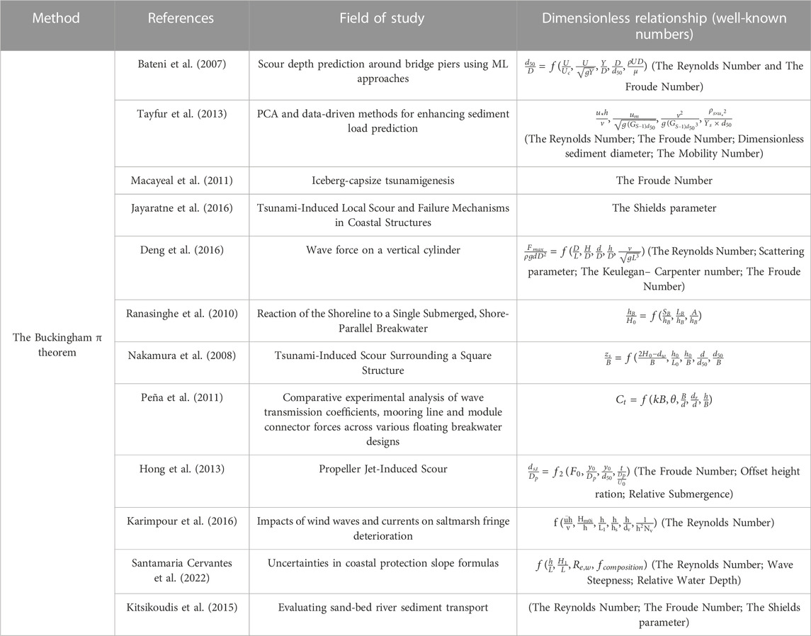
TABLE 3. Comparative overview of various studies utilizing DA and their derived dimensionless parameters.
2.6 Normalization
Normalizing data helps to ensure comparability by transforming it into a common scale, avoiding bias in statistical analyses and allowing for accurate and meaningful results by removing the impact of unit differences, especially when comparing data from different sources. Normalization plays a crucial role in efficient machine and deep learning by ensuring that large numerical inputs are processed effectively (Van Komen et al., 2022). The choice of normalization method depends on the specific requirements of the data and the problem being solved. Some of the famous methods for data normalization are summarized in Table 4.
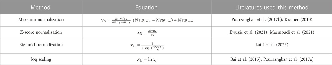
TABLE 4. Well known Normalization techniques used in ML modeling.
In Table 4, the transformed data, referred to as
Min-Max normalization is a technique used to rescale a feature to a specific range, usually between 0 and 1. However, to avoid having zero data in the model, an alternative approach is to expand the range to include values between 0.1 and 0.9. It is a commonly used method for transforming variables so that they are comparable, as it scales the data linearly to a specific range. Through this normalization process, the values in
In coastal phenomena, the relationship between inputs and outputs typically displays nonlinearity, but certain models, such as the M5 model tree, are unable to handle nonlinearity. To address this limitation, M5 models have been implemented using a logarithmic form for both inputs and outputs (i.e., the natural logarithm of inputs and outputs). This logarithmic form is more accurate than a linear formulation because it better captures the nonlinear nature of the contributing parameters (Pourzangbar et al., 2017a; Afsarian et al., 2018). Log scaling entails transforming data points through the application of a logarithmic function. The logarithm maps large values to smaller ones and vice versa, helping to make skewed data more symmetrical and manageable for analysis. The selection of a specific logarithmic function depends on the needs of the data and the analysis to be performed, such as log base 10, log base 2, or natural logarithm. Despite its advantages, normalization may result in a loss of interpretability, increased sensitivity to outliers (as seen in techniques like min-max scaling and z-score), loss of information, dependence on the entire dataset, impacts on categorical features, and varying sensitivity across algorithms.
3 AI learning algorithms and their application in marine/coastal engineering
3.1 Supervised-based ML methods
Supervised ML presents a powerful approach, necessitating labeled data for model training. Its versatility permits its usage across a variety of applications, such as image and speech recognition, natural language processing, and predictive analytics. Common algorithms used in supervised learning encompass linear regression, logistic regression (LR), decision trees, random forests, support vector machines, and neural networks. A key advantage of supervised learning is its capacity to generate precise predictions for novel and unseen data (Jiang et al., 2020). However, it also has certain drawbacks, including the requirement for labeled data, the quality and quantity of the training data, and the potential for overfitting. Despite these challenges, supervised learning is seen as an essential method in ML and data science, demonstrating high accuracy and less computational time compared to physical models. Despite the inherent complexity of marine processes, supervised-based ML models have demonstrated benefits in understanding coastal phenomena, thereby finding extensive application in coastal engineering to drive innovative models and solve intricate problems (as summarized in Table 5). Supervised ML models have been employed to predict wave parameters like significant wave height and period, wave reflection and transmission coefficients (van Gent et al., 2007; Gandomi et al., 2020; Kuntoji et al., 2020), tide levels (Lee, 2004), ocean currents and wind files (James et al., 2018; Shamshirband et al., 2020), prediction of wind Characteristics under future Climate Change scenarios (Yeganeh-Bakhtiary et al., 2022), flood inundation using Gaussian process model (Donnelly et al., 2022) and breakwater stability number and wave overtopping discharge, among others. Various ML models, such as ANN and SVM, can be employed to do these predictions. ML models have also found application in morphological and morphodynamic predictions, including profile elevation, area, and length, based on parameters like wind speed, direction, wave height, and beach angle (Hashemi et al., 2010).
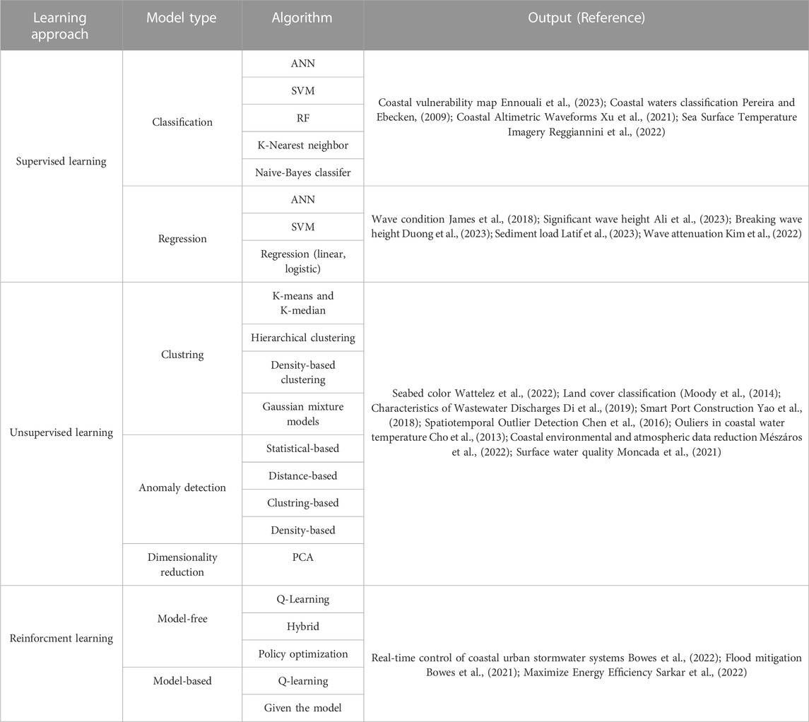
TABLE 5. Various ML learning approaches utilized in coastal studies, along with their associated models and methods.
3.2 Unsupervised-based ML methods
Unsupervised learning is a form of ML that functions without predefined labels or target outcomes (Bishop and Nasrabadi, 2006). Its main purpose is to independently discover patterns, structures, and relationships in data. Common applications include clustering, anomaly detection, and dimensionality reduction. Clustering groups similar data points, anomaly detection spotlights unusual patterns (as detailed in Section 2.3), and dimensionality reduction simplifies the number of features while preserving essential information (as seen in Section 2.4). Algorithms like k-means clustering, hierarchical clustering, PCA, and autoencoders are frequently used in unsupervised learning to identify patterns in data. While unsupervised learning can pose challenges due to the lack of a distinct optimization goal, it still holds a vital position in ML, contributing to advancements in fields such as computer vision, natural language processing, and recommendation systems. In the context of coastal engineering, k-means clustering can be used to classify centroid values for data like the maximum oceanic wind. Average centroid clustering can be obtained from both the previously chosen values and the currently selected clustering data (Baboo and Tajudin, 2013). PCA can be employed in coastal engineering to examine correlation matrices (Roseman et al., 2005) and pinpoint major changes in beach profiles and sand grain distributions (Tsujimoto et al., 2012). Moreover, PCA and hierarchical clustering can help characterize coastal plane shape and hydrodynamics. For instance, the form of arc-shaped coasts, largely influenced by geological structure, can be divided into four broad categories that reflect actual conditions using clustering (Scott et al., 2011). By identifying key data components, PCA can aid in elucidating the underlying patterns and structures of the data.
3.3 Reinforcement-based ML methods
Reinforcement learning (RL) is a type of ML where a program, known as an agent, learns to perform tasks by getting feedback from its environment in the form of rewards or penalties (Rengarajan et al., 2022). The agent executes a series of decisions in a mutable environment, aiming to learn the optimal way (or policy) to maximize rewards over time. This process is typically structured as a Markov Decision Process (MDP), encompassing states, actions, transition functions, and reward functions. There are two main types of reinforcement learning algorithms: model-based and model-free. Model-based RL is like making a map to understand the surroundings. On the other hand, model-free RL does not make a map; it just figures out what to do based on where it is at the moment. So, model-based RL is more about planning ahead, while model-free RL is more about learning on the go (Plaat et al., 2023). Model-free methods, like Q-learning, do not need a model of the environment and calculate the expected total of future rewards for each possible action at each state using the so-called the Bellman equation. Q-learning has been used successfully in many different tasks, which is why it is one of the most commonly used model-free RL algorithms. In coastal engineering, RL can be used to develop control policies to reduce the risk of flooding (Bowes et al., 2021). Deep reinforcement learning (DRL), an advanced form of RL, can be used to control devices that convert wave energy, and has been found to work better than traditional control methods (Anderlini et al., 2020). DRL can also adjust itself to changes in system dynamics, allowing for control even when faults occur. Moreover, RL has been used to maximize the electricity produced by wave energy converters (Zou et al., 2022). In addition, a type of RL called multiagent reinforcement learning can simulate the social and economic effects of sea level rise. This can be a useful tool for planning scenarios, analyzing costs and benefits, and optimizing strategies to adapt to changes (Shuvo et al., 2022).
Table 4 summarizes the various ML learning approaches and their corresponding model types. Each model type utilizes a unique set of algorithms. For instance, in the case of classification tasks, ANNs or SVMs may be utilized. The final column of the table highlights the research studies focusing on each specific learning approach, targeting the investigation of a specific coastal process or event.
3.4 AI contribution to the sustainability of marine environments
Predictive models, such as statistical, numerical, or ML models, play a vital role in marine and coastal engineering to safeguard structures from natural forces. Statistical models use past data to forecast future conditions, while numerical models simulate the event using mathematical equations and formulas. ML models, using artificial intelligence (AI), learn from past data for prediction purposes. Each model has its unique approach and is chosen based on data availability and specific project needs.
Various ML techniques have been implemented in the study of coastal and marine environments. Figure 3, sourced from Scopus, provides a visual representation of the percentage of published papers that used different ML methods since the year 2000. Upon reviewing this figure, it is evident that Principal Components Regression (PCR), Linear Model (LM), Regression Tree (RT), and ANN are the most frequently employed ML algorithms for analyzing coastal and marine phenomena. However, certain ML techniques, such as General Regression Neural Networks (GRNN), M5 model tree, Bayesian Model Averaging method (BMA), Generalized Boosted Regression (GBM), and Extreme Gradient Lift (Xgboost) have been applied less frequently in the investigation of coastal and marine events.
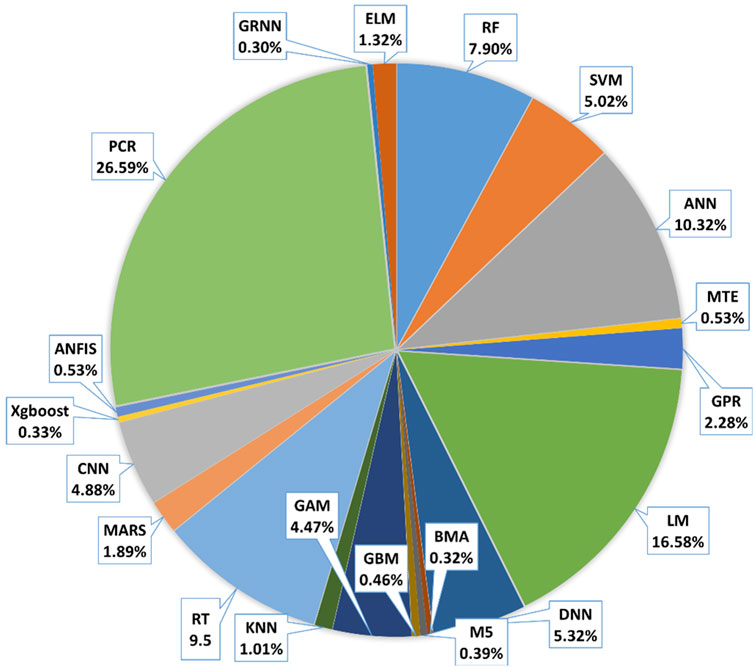
FIGURE 3. Percentage of different ML methods application in coastal and marine environments in terms of the published papers indexed in Scopus.
Figure 4 shows the application trend of different ML approaches for coastal and marine phenomena. Previously, techniques such as Deep Neural Networks (DNN), Convolutional Neural Networks (CNN), and RF were sparingly employed in diverse studies. However, there has been a significant increase in their use over the past 5 years, demonstrating a growing reliance on these methods in recent research.
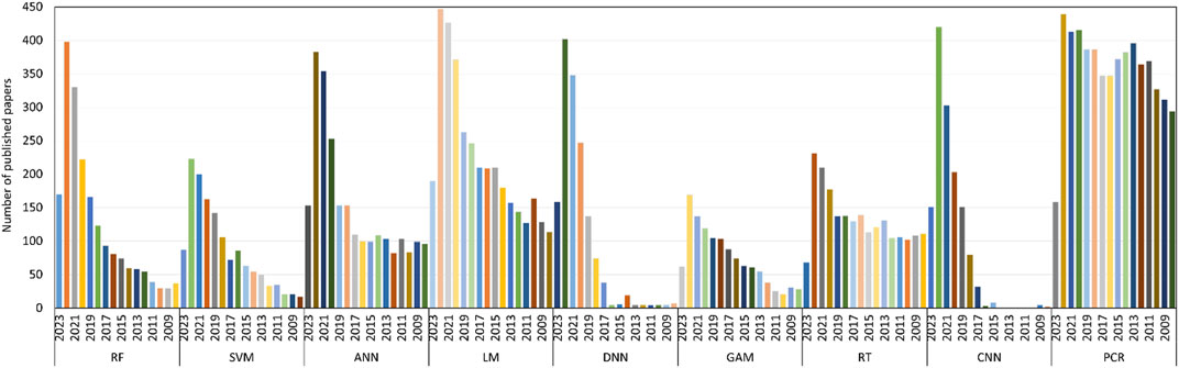
FIGURE 4. The trend of varios ML algorithms in coastal and marine applicatins.
Figure 5 illustrates the trend of various ML algorithms since 2008 in coastal and marine applications. Some methods are not frequently used which are colored in red (these low-important approaches are not reported in Figure 4).
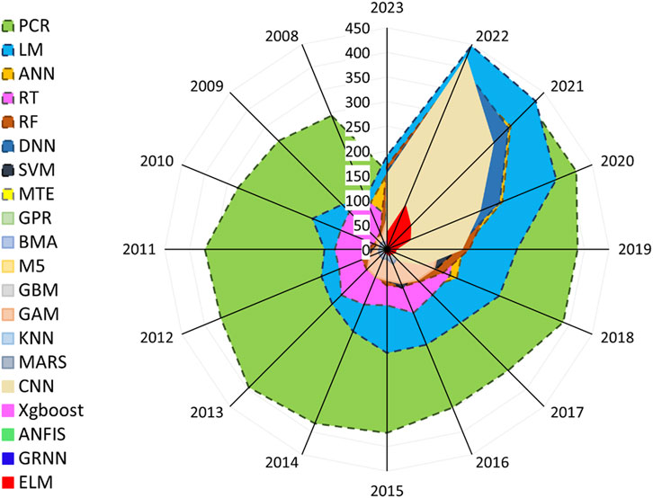
FIGURE 5. Annual publication trends of papers implementing ML methods for predicting coastal and marine phenomena, as extracted from scopus.
3.4.1 Prediction of oceanographic and morphologic parameters
Researchers use ML algorithms and soft computing techniques to predict oceanographic and morphological parameters, as shown in Figure 6. These methods include ANNs, SVMs, Support Vector Regression (SVR), Fuzzy Logic (FL), evolutionary algorithms, such as Genetic Programming (GP) and DTs, among others. Predictive models are widely used in oceanography and coastal management. Their accuracy critically depends on several factors. These include the dataset used for training, the type and configuration of the ML model, tuning parameters, termination condition, and input and output parameters. It is important to note that specific algorithms, with carefully adjusted parameters, are particularly valuable in various research endeavors, depending on the problem being addressed.
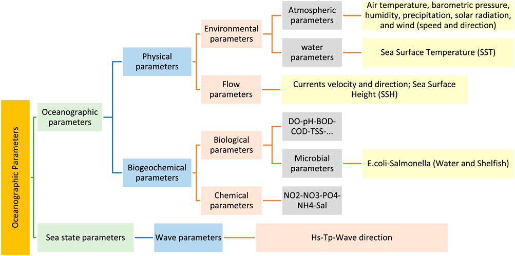
FIGURE 6. Oceanographic Parameters predicted by ML algoithms.
ANNs, SVRs, M5 decision tree algorithm, and Recurrent Neural Networks (RNNs) including Long-Short-Term Memory (LSTM) models are used to predict wave heights, as per studies by Duong et al. (2023) and Rizianiza and Aisjah (2015). These ML techniques have shown reliable wave prediction capabilities, maintaining accuracy up to 72 h ahead (Jain and Deo, 2008). The use of intact structural data for predicting significant wave heights has been explored, with emphasis on the critical role of data quality in training ANNs for wave height predictions (Ciortan and Rusu, 2018; Demetriou et al., 2021). ANNs have also been implemented to estimate wave breaking heights considering various factors like seabed slope, water depth, and deep-sea wavelength (Duong et al., 2023). In the field of marine energy forecasting, researchers have used multi-class classification methods with ordinal classifiers, such as SVOREX and SVORIM yielding precise results (Fernández et al., 2015). RNN, especially LSTM models, have been employed to predict motion responses in irregular wave patterns (Kagemoto, 2020). Table 6 provides a summary of the top 10 highly-cited papers focused on predicting significant wave height using ML algorithms. The majority of these studies used meteorological data and past wave height as input parameters. The results demonstrate that LSTM neural networks, ANN, kernel-based predictors like SVM and SVR, as well as decision trees, are capable of accurately predicting wave height.
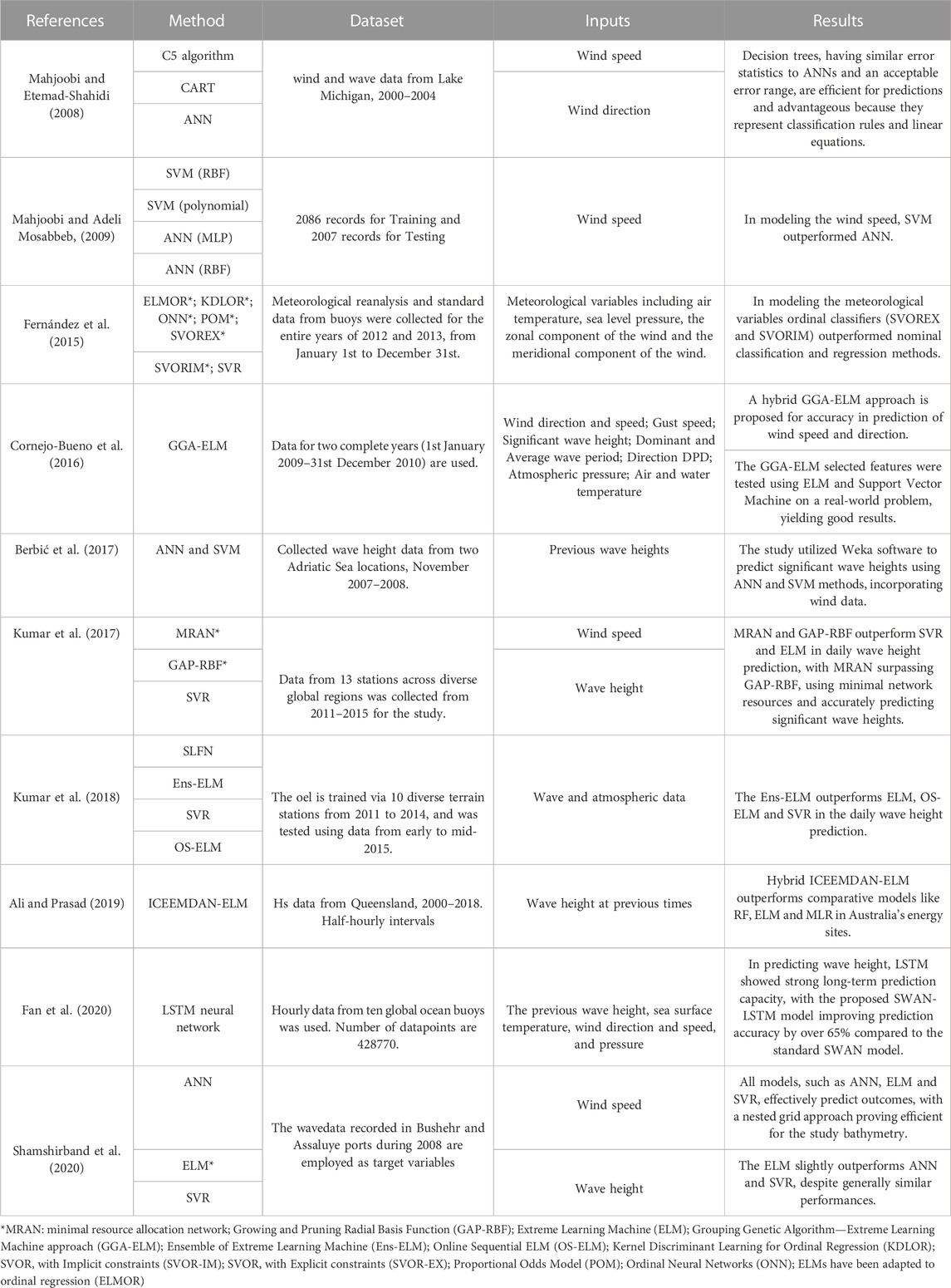
TABLE 6. Details of the selected reviewed papers, where the ML methods were used to predict the wave height.
To enhance understanding of the effectiveness of various ML methods in predicting wave height, visual representations of the correlation coefficient and Root Mean Square Error (RMSE) values for different ML techniques applied across multiple data sets have been created (Figure 7). To achieve this, we carefully selected studies that used several ML methods for wave height predictions, ensuring each study used a consistent dataset. This allowed for a visual representation of the performance of these ML techniques with specific datasets. By comparing the overall performance of these ML models across various datasets, certain conclusions can be drawn.
• ANN and SVR algorithms are commonly used in predicting wave height.
• The count of neurons present in the hidden layers of ANNs slightly influences the precision of the model.
• Integrated algorithms, like ICEEMDAN-ELM, exhibit superior performance in terms of accuracy and error indices compared to other ML methods.
• There has been a significant increase in the adoption of ML algorithms, especially integrated algorithms, in recent years (see Figure 8).

FIGURE 7. Comparison of CC (upper panel) and RMSE (lower panel) across different ML approaches and datasets. Each color symbolizes a unique study. Results are extracted from Makarynskyy et al. (2005); Mahjoobi and Etemad-Shahidi (2008); Mahjoobi and Adeli Mosabbeb, (2009); Cornejo-Bueno et al. (2016); Berbić et al. (2017); Akbarifard and Radmanesh (2018); Kumar et al. (2018); Nikoo et al. (2018); Ali and Prasad (2019); Shamshirband et al. (2020); Kaloop et al. (2020). The abbreviations are: Online sequential ELM (OSELM), Extreme Learning Machine (ELM), Improved Complete Ensemble Empirical Mode Decomposition method with Adaptive Noise (ICEEMDAN), Online Sequential (OS), RF, Grouping Genetic Algorithm (GGA).
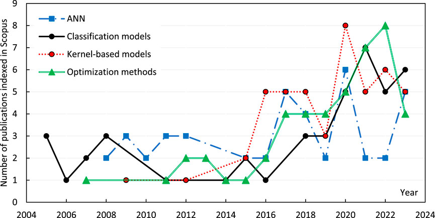
FIGURE 8. Wave height prediction using different ML algorithms during 2005–2023.
The M5 decision tree algorithm, ANNs, and gradient boosting decision trees serve as robust tools for predicting wave overtopping discharge on coastal infrastructure such as breakwaters. When focusing on wave overtopping and runup, the M5 decision tree algorithm exhibits promising capabilities for predicting runup waves, taking into account laboratory data and multiple parameters (Abolfathi et al., 2016). ANNs are also used to predict wave reflection and transmission coefficients (Zanuttigh et al., 2016; Formentin et al., 2017). It has been proven that gradient boosting decision trees, as a novel ML technique, has improved the accuracy of predicting average wave overtopping discharges by nearly threefold in comparison to traditional neural networks (den Bieman et al., 2020). Kernel-based approaches, such as Gaussian Process Regression (GPR) and SVR, have also been utilized in predicting wave overtopping, with GPR showing superior performance over ANNs and empirical formulas (Hosseinzadeh et al., 2021).
The measurement of Sea Surface Temperature (SST) is vital for understanding the global climate. It significantly contributes to climate modeling, weather forecasting, and studies on marine ecosystems. Accurately predicting SST can aid in mitigating the environmental harm resulting from rising water temperatures due to human-induced climate change. This prediction not only benefits marine ecosystems but also preserves coastal economies and the broader coastal environment (Choi et al., 2023). LSTM neural networks have proven effective in forecasting SST, showing enhanced performances when the right amount of input data is used (Xu et al., 2020). Multivariate LSTM models, which take into account factors such as wind speed and sea-level air pressure alongside SST, have demonstrated superior results compared to univariate models that only factor in SST (Balogun and Adebisi, 2021). Traditional ML models have been studied for spatio-temporal time series prediction, highlighting the importance of spatial data. Among these, the LSTM model emerged as the most efficient, showing a 25% improvement in forecasting performance (based on RMSE) when spatial information was incorporated (Kartal, 2023). Research indicates that LSTMs, whether using single or multiple variables, surpass other ML models in predicting SST (Xu et al., 2020; Kartal, 2023).
Moreover, accurate predictions of coastal sediment transport are crucial for managing coastal erosion and development, with researchers traditionally estimating sediment transport using experimental methods. Artificial intelligence-based methods potentially improve decision-making for managing coastal erosion and development (Bakhtyar et al., 2008; Kabiri-Samani et al., 2011), given the importance of selecting valid input data and appropriate activation functions (Pourzangbar, 2012; Yeganeh-bakhtiary et al., 2012). Artificial intelligence and ML methods, such as Adaptive Network Based Fuzzy Inference Systems (ANFIS), Fuzzy Inference System (FIS), CERC (Coastal Engineering Research Center), Walton-Bruno (WB), Van Ridge (VR), and ANNs, have been employed to model sediment transport, with ANFIS showing higher accuracy and reliability for estimating longshore sediment transport rates (LSTR) (Bakhtyar et al., 2008; Hashemi et al., 2010). SVR has also been employed, demonstrating superiority over neural networks when the dataset is small or the relationships are linear or non-linear but with a clear margin (Dezvareh and Shafaghat, 2020). Deep learning models, like ANNs, have been developed to address the shortcomings of numerical models in analyzing simultaneous sand and sediment transport (Kim and Aoki, 2021).
3.4.2 Classification models
Classification involves categorizing items or data into groups based on their features, and is crucial in fields such as statistics, ML and data analysis. The goal is to create models that predict the class of new items by identifying patterns in their features. SVM was introduced in the 1990s, RF in the early 2000s, and LR has roots going back to the 19th century. These algorithms are capable of executing simple tasks such as recognition and classification (Lou et al., 2021). In addition to these algorithms, a variety of other classification algorithms, including naive Bayes classifier, DTs, and K-Nearest Neighbors, have been utilized in remote sensing and in situ data analysis to enhance the understanding and monitoring of the environment. Table 7 summarizes the most well-known classification models used in coastal and marine engineering. These algorithms have proven effective in unraveling complex environmental data and facilitating informed decision-making (Tsiakos and Chalkias, 2023). Accordingly, the most famous classification methods are:
• SVM (Cortes and Vapnik, 1995): focuses on training samples near the optimal class boundary, aiming to maximize the margin between support vectors. Fundamentally, it is a binary classifier, and the processing time is managed by applying the classifier to every class combination.
• Regression Tree (RT) (Goldstein et al., 2019): break down prediction tasks into binary splits, forming a tree structure. This tool excels at classification tasks and enables an understanding of the influence of input variables. However, RTs may not be as effective for continuous variables and are prone to overfitting if not properly pruned. Accuracy can be boosted by merging small sequential RT models, giving more weight to poorly predicted data.
• Decision Trees (Pal and Mather, 2003): easy to understand, DTs recursively split data. They can use categorical data and perform classification quickly. However, DTs may suffer from overfitting and non-optimal solutions, which can be addressed through pruning.
• RF (Breiman, 2001): an ensemble classifier using multiple DTs to overcome their limitations. Each tree uses a random subset of training data and features, resulting in a more accurate ensemble. RF classifiers are known for their speed, resistance to overfitting, and ability to handle multicollinearity. They can also assess the importance of variables, although they may be sensitive to certain sampling strategies (Belgiu and Drăgu, 2016).
• Kernel and Nearest Neighbor (K-NN) classifier (Altman, 1992): The K-NN classifier is distinct from other classifiers because it does not create a model during the training phase. Instead, every unclassified sample is directly compared with the original training data.
• Naive-Bayes classifer: it is a classification algorithm that is based on Bayes’ theorem and assumes that the presence or absence of one feature is independent of the presence or absence of other features. It learns the probability distribution of features and corresponding labels from a training dataset and uses it to classify new examples. This algorithm is widely used in applications that have many features and large datasets, such as text classification, sentiment analysis, and spam filtering. The Naive Bayes classifier is computationally efficient and can handle high-dimensional data well.
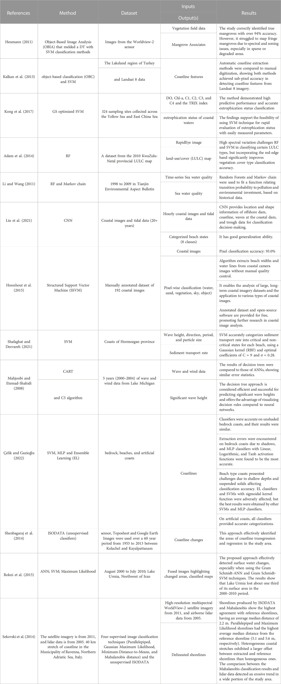
TABLE 7. Overview of highly-cited literature studies (extracted from Scopus) on classification models in coastal and marine phenomena.
KNN classifier has been used in various marine-related projects. For the design of marine hydrokinetic turbines, KNN was used to identify and categorize the severity of the rotor blade pitch imbalance encountered by marine current turbines. This approach was found useful for fault detection and severity classification (Freeman et al., 2021). In ocean surface current forecasting, KNN was used as an alternate method (Jirakittayakorn et al., 2017). The KNN algorithm proved capable of forecasting future surface currents up to 24 h in advance. The KNN approach was compared with other prediction techniques such as ARIMA, exponential smoothing, and LSTM, and it was found that the KNN model had the highest accuracy. KNN was one of the six ML classifiers used to generate precise geographic estimates of seabed substrate and seabed habitat mapping (Diesing and Stephens, 2015; Leon et al., 2020). The accuracy of the predictions was evaluated using ground-truth sample data segmented into classes of seabed substrate. In coastal hazards projection, KNN was used to project dangers using several representative concentration route climate change scenarios, regional climate models, and sea level rise ratios (Park and Lee, 2020). Seafloor classification is another marine-related project where KNN was used along with ANN to class the structure of the seafloor and to pinpoint potential anthropogenic effects on delicate benthic assemblages (Gauci et al., 2016). Finally, in sea-land segmentation, KNN was used to produce a pixel-level, sea-land segmentation of the scene based on the Doppler bandwidth of a returns vector in maritime surveillance radars (Shui et al., 2020).
The Naive Bayes classifier is a machine learning algorithm commonly utilized in various applications to enhance model accuracy. A prominent application of the Naive Bayes classifier involves predicting water quality classes utilizing seven popular Water Quality Index (WQI) models (Uddin et al., 2023). There is some confusion about the proper classification of water quality due to differing techniques used in current WQI models. To address this, the Naive Bayes was compared with other ML classifiers. These included SVM, Random Forest, K-Nearest Neighbor, and Gradient Boosting. The goal was to determine the best classifier for evaluating water quality. Another application of the Naive Bayes classifier is in detecting small-scale assemblages of drifting vegetation and beach cast in Germany’s Baltic coast (Uhl et al., 2022). To obtain the best classification results, the classifier was used as part of an ensemble of five classifiers, including a RF, CART, SVM, and stochastic gradient boosting classifier to predict tropical Cyclone based on multi-model fusion across Indian coastal region (Varalakshmi et al., 2021). In all applications, the Naive Bayes classifier was effective in improving the accuracy of the models, particularly in predicting the quality of coastal water and detecting small-scale assemblages of drifting vegetation and beach cast. Its versatility and usefulness in different domains make it a popular choice for improving the accuracy of models in various applications.
Given coastaline extraction from satellite images, three well known methods including image processing techniques, unsupervised classifiers and supervised classifiers have been implemented. Shenbagaraj et al. (2014) employed visual interpretation and ISODATA (Iterative Self-Organizing Data Analysis Technique) classification techniques to extract shorelines from Landsat Thematic Mapper (TM), Enhanced Thematic Mapper Plus (ETM+) sensor images, Toposheet and Google Earth Images spanning a 60-year period from 1953 to 2013 between Kolachel and Kayalpattanam. This approach effectively identified the areas of coastline transgression and regression in the study area. Supervised classifiers such as Maximum Likelihood (Rokni et al., 2015), SVM & ANN & EL (Çelik and Gazioğlu, 2022), RF (Bayram et al., 2017), Minimum-Distance-to-Means, and Mahalanobis distance (Sekovski et al., 2014) also have been employed to classify and detect the coastline position based on the satellite images. As depicted in Figure 9, the average median distance of all shorelines, observed in relation to the reference, suggests that the shorelines produced by the ISODATA and Mahalanobis methods demonstrate the best alignment, with a discrepancy of 2.2 m, thereby being closer to the reference than other methods. Conversely, the Parallelepiped and Maximum Likelihood methods resulted in shorelines with the highest average median distance from the reference shoreline, measuring 5.1 m and 5.6 m respectively.
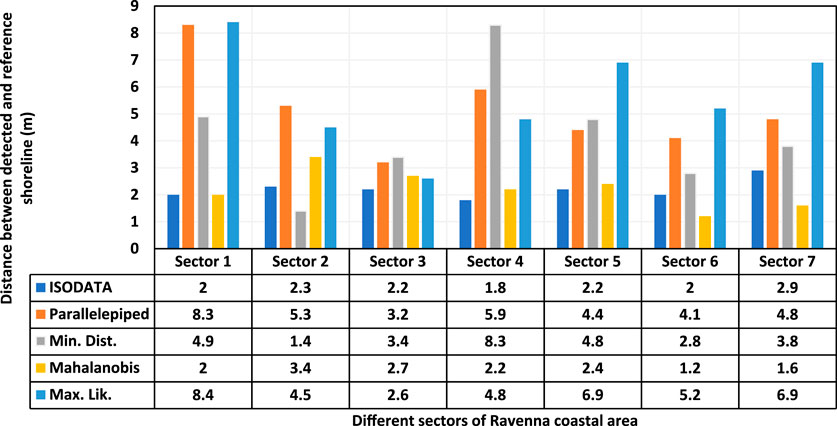
FIGURE 9. Comparison of different classifiers’ performance in detecting shoreline position given the reference shoreline position at different sectors of Ravenna coastal area (Sekovski et al., 2014). Sector 1: Bellocchio Channel. To Reno River; sector 2: Reno River to Destra Reno channel; sector 3: Destra Reno channel to Lamone River; sector 4: Lamone River to Porto Corsini; sector 5: Marina di Ravenna to Fiumi Uniti River; sector 6: Fiumi Uniti River to Bevano stream; sector 7: Bevano stream to Savio River.
4 Summary and conclusion
This study provides a comprehensive review of machine learning applications to model the marine and coastal environments, with comprehensive coverage from data preprocessing to the application of different models. The review indicates that appropriately implemented and optimized ML methods can significantly contribute to marine and coastal sustainability through developing accurate and robust models for prediction of wave height, oceanographic parameters, and sediment transport, image processing, optimization of coastal and marine structures design.
Here are some insights based on your review:
1. Dependence on data quality: the study concludes by reminding us that the efficacy of ML models heavily relies on factors such as the quality of datasets, the type and configuration of the ML model, and tuning parameters. It reemphasizes the importance of sound data science practices in applying ML.
2. Exploitation of data: this paper underlines the importance of data preprocessing, including data cleaning, dimensionality reduction, and normalization in machine learning models. This emphasizes the pivotal role of quality data in the effectiveness of ML applications in modelling phenomena such as wave patterns, coastal erosion, and sediment transport in marine and coastal environments.
3. Diverse machine learning approaches: the current paper is examined three primary types of ML including supervised, unsupervised and reinforcement learning, and their respective applications in marine and coastal science. Supervised learning, using algorithms such as decision trees and neural networks, leverages labeled data to predict parameters like wave height and wind speed, and make morphodynamic predictions. Unsupervised learning, on the other hand, independently discovers patterns and relationships in data for tasks like clustering and anomaly detection, and has been employed to classify wind values and examine beach profiles. Reinforcement learning, operating on a reward or penalty system, plays a vital role in devising control policies and planning for future scenarios in areas like flood risk reduction and wave energy conversion. Various ML methods such as PCR, LM, RT, and ANN are instrumental in facilitating these applications.
4. Classification algorithms: classification algorithms such as Kernel- and Tree-based models play crucial roles in environmental data interpretation and decision-making. SVM is known for its binary classification capabilities, while RT and DT provide swift classification and a better understanding of input variables. RF offers robustness against overfitting and efficiently manages multicollinearity. The KNN classifier performs well in comparing unclassified samples with training data. Naive Bayes, using Bayes’ theorem, efficiently processes and analyzes high-dimensional data and is often used in predicting water quality and tropical cyclone trajectories.
5. Application of ML: from forecasting oceanographic and morphologic parameters to estimating longshore sediment transport rates, the use of ML significantly enhances the capacity for prediction and understanding of marine and coastal environments. ANNs and SVR are frequently used for wave height predictions. Their accuracy and reliability help in crucial areas such as managing coastal erosion and development. The prediction of SST using ML, specifically LSTM neural networks, has shown great promise. Accurate SST prediction can contribute significantly to climate modeling, weather forecasting and the preservation of marine ecosystems. ANFIS has shown accuracy and reliability in estimating longshore sediment transport rates, which is essential for managing coastal erosion and development.
6. The growing role of new techniques: the rising prominence of deep neural networks, convolutional neural networks, and random forests is indicative of the evolution of the field, and the increasing complexity of the problems being addressed. These advanced techniques often deliver superior performance and can manage more complex and high-dimensional datasets. Integrated algorithms such as ICEEMDAN-ELM exhibit superior performance. The adoption of ML algorithms has seen a significant increase in recent years.
4.1 Recommendations for future research endeavours
• Developing hybrid models: the employment of combined and hybrid models has exhibited significant success, notably in addressing multifaceted issues. Eslaminezhad et al. (2022) advanced the efficiency of tree-structured machine learning models in determining the crucial parameters for forecasting flood susceptibility and constructing flood susceptibility maps, through the incorporation of the BPSO algorithm.
• Developoing physical-based machine learning: it is apparent that machine learning models do not adequately consider the actual physical elements of the problem. Consequently, the prospect of integrating physical-based machine learning approaches is recommended for further contemplation.
• Implementing domain adaptation techniques: to address the regional restrictions inherent in existing models, it might be prudent to consider the application of domain adaptation techniques.
• Evaluating models’ uncertainty: it is essential to acknowledge that inherent uncertainty is a fundamental aspect of any model. Thus, it is proposed that the models’ uncertainty be consistently documented, and appropriate methodologies be utilized to alleviate it.
• Development of appropriate scaling techniques: by developing appropriate scaling techniques, one ensures that all features contribute equally to the final prediction, thereby improving the performance of the machine learning model.
Author contributions
AP: Supervision, Compilation and Integration of Data, Data Curation, Software, Validation, Visualization, Writing—Review and Editing. MJ: Literature Search, Information Provision, Writing—Review and Editing. MB: Supervision, Writing—Review and Editing, Funding Acquisition, Project Administration. All authors contributed to the article and approved the submitted version.
Conflict of interest
The authors declare that the research was conducted in the absence of any commercial or financial relationships that could be construed as a potential conflict of interest.
Publisher’s note
All claims expressed in this article are solely those of the authors and do not necessarily represent those of their affiliated organizations, or those of the publisher, the editors and the reviewers. Any product that may be evaluated in this article, or claim that may be made by its manufacturer, is not guaranteed or endorsed by the publisher.
References
Abolfathi, S., Yeganeh-Bakhtiary, A., Hamze-Ziabari, S. M., and Borzooei, S. (2016). Wave runup prediction using M5′ model tree algorithm. Ocean. Eng. 112, 76–81. doi:10.1016/J.OCEANENG.2015.12.016
Adam, E., Mutanga, O., Odindi, J., and Abdel-Rahman, E. M. (2014). Land-use/cover classification in a heterogeneous coastal landscape using RapidEye imagery: evaluating the performance of random forest and support vector machines classifiers. Int. J. Remote Sens. 35, 3440–3458. doi:10.1080/01431161.2014.903435
Afsarian, F., Saber, A., Pourzangbar, A., Olabi, A. G., and Khanmohammadi, M. A. (2018). Analysis of recycled aggregates effect on energy conservation using M5″ model tree algorithm. Energy 156, 264–277. doi:10.1016/j.energy.2018.05.099
Agarwal, P., and Manuel, L. (2008). Extreme loads for an offshore wind turbine using statistical extrapolation from limited field data. Wind Energy 11, 673–684. doi:10.1002/we.301
Agrafiotis, P., Skarlatos, D., Georgopoulos, A., and Karantzalos, K. (2019). DepthLearn: learning to correct the refraction on point clouds derived from aerial imagery for accurate dense shallow water bathymetry based on SVMs-fusion with LiDAR point clouds. Remote Sens. 11, 2225. doi:10.3390/rs11192225
Akbarifard, S., and Radmanesh, F. (2018). Predicting sea wave height using Symbiotic Organisms Search (SOS) algorithm. Ocean. Eng. 167, 348–356. doi:10.1016/J.OCEANENG.2018.04.092
Ali, M., and Prasad, R. (2019). Significant wave height forecasting via an extreme learning machine model integrated with improved complete ensemble empirical mode decomposition. Renew. Sustain. Energy Rev. 104, 281–295. doi:10.1016/J.RSER.2019.01.014
Ali, M., Prasad, R., Xiang, Y., Jamei, M., and Yaseen, Z. M. (2023). Ensemble robust local mean decomposition integrated with random forest for short-term significant wave height forecasting. Renew. Energy 205, 731–746. doi:10.1016/J.RENENE.2023.01.108
Altman, N. S. (1992). An introduction to kernel and nearest-neighbor nonparametric regression. Am. Statistician 46, 175–185. doi:10.1080/00031305.1992.10475879
Anderlini, E., Husain, S., Parker, G. G., Abusara, M., and Thomas, G. (2020). Towards real-time reinforcement learning control of a wave energy converter. J. Mar. Sci. Eng. 8, 845. doi:10.3390/jmse8110845
Arslan, O., Akyürek, Ö., Kaya, Ş., and Şeker, D. Z. (2020). Dimension reduction methods applied to coastline extraction on hyperspectral imagery. Geocarto Int. 35, 376–390. doi:10.1080/10106049.2018.1520920
Ba-Alawi, A. H., Vilela, P., Loy-Benitez, J., Heo, S. K., and Yoo, C. K. (2021). Intelligent sensor validation for sustainable influent quality monitoring in wastewater treatment plants using stacked denoising autoencoders. J. Water Process Eng. 43, 102206. doi:10.1016/j.jwpe.2021.102206
Baboo, S. S., and Tajudin, K. (2013). “Clustering centroid finding algorithm (CCFA) using spatial temporal data mining concept,” in 2013 International Conference on Pattern Recognition, Informatics and Mobile Engineering 2013, Salem, India, February 21–22, 2013 (IEEE (Institute of Electrical and Electronics Engineers), 30–36. doi:10.1109/ICPRIME.2013.6496443
Bai, Y., Cai, W. J., He, X., Zhai, W., Pan, D., Dai, M., et al. (2015). A mechanistic semi-analytical method for remotely sensing Sea Surface pCO2 in river-dominated coastal oceans: a case study from the east China sea. J. Geophys. Res. Oceans 120, 2331–2349. doi:10.1002/2014JC010632
Bakhtyar, R., Ghaheri, A., Yeganeh-Bakhtiary, A., and Baldock, T. E. (2008). Longshore sediment transport estimation using a fuzzy inference system. Appl. Ocean Res. 30, 273–286. doi:10.1016/J.APOR.2008.12.001
Balogun, A. L., and Adebisi, N. (2021). Sea level prediction using ARIMA, SVR and LSTM neural network: assessing the impact of ensemble ocean-atmospheric processes on models’ accuracy. Geomatics, Nat. Hazards Risk 12, 653–674. doi:10.1080/19475705.2021.1887372
Bateni, S. M., Borghei, S. M., and Jeng, D. S. (2007). Neural network and neuro-fuzzy assessments for scour depth around bridge piers. Eng. Appl. Artif. Intell. 20, 401–414. doi:10.1016/j.engappai.2006.06.012
Bayram, B., Erdem, F., Akpinar, B., Ince, A. K., Bozkurt, S., Catal Reis, H., et al. (2017). The efficiency of random forest method for shoreline extraction from landsat-8 and gokturk-2 imageries. ISPRS Ann. Photogrammetry, Remote Sens. Spatial Inf. Sci., 141–145. doi:10.5194/isprs-annals-IV-4-W4-141-2017
Belgiu, M., and Drăguţ, L. (2016). Random forest in remote sensing: a review of applications and future directions. ISPRS J. Photogrammetry Remote Sens. 114, 24–31. doi:10.1016/J.ISPRSJPRS.2016.01.011
Berbić, J., Ocvirk, E., Carević, D., and Lončar, G. (2017). Application of neural networks and support vector machine for significant wave height prediction. Oceanologia 59, 331–349. doi:10.1016/J.OCEANO.2017.03.007
Beuzen, T., Goldstein, E. B., and Splinter, K. D. (2019). Ensemble models from machine learning: an example of wave runup and coastal dune erosion. Nat. Hazards Earth Syst. Sci. 19, 2295–2309. doi:10.5194/nhess-19-2295-2019
Booij, N., Holthuijsen, L. H., and Ris, R. C. (1997). The swan wave model for shallow water. Coast. Eng. 1996. doi:10.1061/9780784402429.053
Bowes, B. D., Tavakoli, A., Wang, C., Heydarian, A., Behl, M., Beling, P. A., et al. (2021). Flood mitigation in coastal urban catchments using real-time stormwater infrastructure control and reinforcement learning. J. Hydroinformatics 23, 529–547. doi:10.2166/HYDRO.2020.080
Bowes, B. D., Wang, C., Ercan, M. B., Culver, T. B., Beling, P. A., and Goodall, J. L. (2022). Reinforcement learning-based real-time control of coastal urban stormwater systems to mitigate flooding and improve water quality. Environ. Sci. Water Res. Technol. 8, 2065–2086. doi:10.1039/d1ew00582k
Brown, J. M., Yelland, M. J., Pullen, T., Silva, E., Martin, A., Gold, I., et al. (2021). Novel use of social media to assess and improve coastal flood forecasts and hazard alerts. Sci. Rep. 11, 13727. doi:10.1038/s41598-021-93077-z
Çelik, O. İ., and Gazioğlu, C. (2022). Coast type based accuracy assessment for coastline extraction from satellite image with machine learning classifiers. Egypt. J. Remote Sens. Space Sci. 25, 289–299. doi:10.1016/J.EJRS.2022.01.010
Chandola, V., Banerjee, A., and Kumar, V. (2009). Anomaly detection: a survey. ACM Comput. Surv. 41, 1–58. doi:10.1145/1541880.1541882
Chen, J., Abbady, S., and Duggimpudi, M. B. (2016). Spatiotemporal outlier detection: did buoys tell where the hurricanes were? Pap. Appl. Geogr. 2, 298–314. doi:10.1080/23754931.2016.1149874
Chen, W., and Ma, W. (2010). “Applications based on genetic neural network model of Lianyungang marine water quality optimization techniques and algorithms Technology”. 2010 International Conference of Information Science and Management Engineering 2010 1, 526–529. doi:10.1109/ISME.2010.253
Cho, H. Y., Oh, J. H., Kim, K. O., and Shim, J. S. (2013). Outlier detection and missing data filling methods for coastal water temperature data. J. Coast. Res. 165, 1898–1903. doi:10.2112/si65-321.1
Choi, H. M., Kim, M. K., and Yang, H. (2023). Deep-learning model for sea surface temperature prediction near the Korean Peninsula. Deep Sea Res. Part II Top. Stud. Oceanogr. 208, 105262. doi:10.1016/J.DSR2.2023.105262
Ciortan, S., and Rusu, E. (2018). Prediction of the wave power in the Black Sea based on wind speed using artificial neural networks. E3S Web Conf. 51, 01006. doi:10.1051/e3scconf/20185101006
Copernicus (2023). The copernicus marine service. Available at: https://marine.copernicus.eu/about.
Cornejo-Bueno, L., Nieto-Borge, J. C., García-Díaz, P., Rodríguez, G., and Salcedo-Sanz, S. (2016). Significant wave height and energy flux prediction for marine energy applications: a grouping genetic algorithm – extreme learning machine approach. Renew. Energy 97, 380–389. doi:10.1016/J.RENENE.2016.05.094
Cortes, C., and Vapnik, V. (1995). Support-vector networks. Mach. Learn. 20, 273–297. doi:10.1023/A:1022627411411
Cuadra, L., Salcedo-Sanz, S., Nieto-Borge, J. C., Alexandre, E., and Rodríguez, G. (2016). Computational intelligence in wave energy: comprehensive review and case study. Renew. Sustain. Energy Rev. 58, 1223–1246. doi:10.1016/j.rser.2015.12.253
Daranda, A., and Dzemyda, G. (2020). Navigation decision support: discover of vessel traffic anomaly according to the historic marine data. Int. J. Comput. Commun. CONTROL 15. doi:10.15837/IJCCC.2020.3.3864
Davidson, M. A., Bird, P. A. D., Bullock, G. N., and Huntley, D. A. (1996). A new non-dimensional number for the analysis of wave reflection from rubble mound breakwaters. Coast. Eng. 28, 93–120. doi:10.1016/0378-3839(96)00012-9
Demetriou, D., Michailides, C., Papanastasiou, G., and Onoufriou, T. (2021). Coastal zone significant wave height prediction by supervised machine learning classification algorithms. Ocean. Eng. 221, 108592. doi:10.1016/j.oceaneng.2021.108592
den Bieman, J. P., Wilms, J. M., van den Boogaard, H. F. P., and van Gent, M. R. A. (2020). Prediction of mean wave overtopping discharge using gradient boosting decision trees. Water 12. doi:10.3390/W12061703
Deng, Y., Yang, J., Zhao, W., Li, X., and Xiao, L. (2016). Freak wave forces on a vertical cylinder. Coast. Eng. 114, 9–18. doi:10.1016/j.coastaleng.2016.03.007
Deroliya, P., Ghosh, M., Mohanty, M. P., Ghosh, S., Rao, K. D., and Karmakar, S. (2022). A novel flood risk mapping approach with machine learning considering geomorphic and socio-economic vulnerability dimensions. Sci. Total Environ. 851, 158002. doi:10.1016/j.scitotenv.2022.158002
Dezvareh, R., and Shafaghat, M. (2020). Predicting the sediment rate of Nakhilo Port using artificial intelligence. Int. J. Coast. offshore Eng. 4 (2), 41–49. doi:10.22034/IJCOE.2020.149345
Di, Z., Chang, M., Guo, P., Li, Y., and Chang, Y. (2019). Using real-time data and unsupervised machine learning techniques to study large-scale spatio-temporal characteristics of wastewater discharges and their influence on surface water quality in the Yangtze River Basin. WaterSwitzerl. 11, 1268. doi:10.3390/w11061268
Diesing, M., and Stephens, D. (2015). A multi-model ensemble approach to seabed mapping. J. Sea Res. 100, 62–69. doi:10.1016/j.seares.2014.10.013
Dogan, G., Ford, M., and James, S. (2021). “Predicting ocean-wave conditions using buoy data supplied to a hybrid RNN-LSTM neural network and machine learning models,” in Proceedings of the 2021 IEEE International Conference on Machine Learning and Applied Network Technologies, Soyapango, El Salvador, December 16–17, 2021 (IEEE (Institute of Electrical and Electronics Engineers)). ICMLANT 2021. doi:10.1109/ICMLANT53170.2021.9690528
Donnelly, J., Abolfathi, S., Pearson, J., Chatrabgoun, O., and Daneshkhah, A. (2022). Gaussian process emulation of spatio-temporal outputs of a 2D inland flood model. Water Res. 225, 119100. doi:10.1016/j.watres.2022.119100
Duong, N. T., Tran, K. Q., Luu, L. X., and Tran, L. H. (2023). Prediction of breaking wave height by using artificial neural network-based approach. Ocean. Model. 182, 102177. doi:10.1016/J.OCEMOD.2023.102177
El-Haddad, B. A., Youssef, A. M., Pourghasemi, H. R., Pradhan, B., El-Shater, A. H., and El-Khashab, M. H. (2021). Flood susceptibility prediction using four machine learning techniques and comparison of their performance at Wadi Qena Basin, Egypt. Nat. Hazards 105, 83–114. doi:10.1007/s11069-020-04296-y
El-Rahman, S. A. (2016). “Hyperspectral imaging classification using ISODATA algorithm: big data challenge”. in Proceedings - 2015 5th International Conference on e-Learning, Manama, Bahrain, October 18–20, 2015 (IEEE (Institute of Electrical and Electronics Engineers)). doi:10.1109/ECONF.2015.39
Elsayed, S., Ibrahim, H., Hussein, H., Elsherbiny, O., Elmetwalli, A. H., Moghanm, F. S., et al. (2021). Assessment of water quality in lake qaroun using ground-based remote sensing data and artificial neural networks. Water 13, 3094. doi:10.3390/w13213094
Emmanouil, S., Aguilar, S. G., Nane, G. F., and Schouten, J. J. (2020). Statistical models for improving significant wave height predictions in offshore operations. Ocean. Eng. 206, 107249. doi:10.1016/j.oceaneng.2020.107249
Ennouali, Z., Fannassi, Y., Lahssini, G., Benmohammadi, A., and Masria, A. (2023). Mapping coastal vulnerability using machine learning algorithms: a case study at north coastline of sebou estuary, Morocco. Regional Stud. Mar. Sci. 60, 102829. doi:10.1016/J.RSMA.2023.102829
Ester, M., Kriegel, H.-P., Sander, J., and Xu, X. (1996). “A density-based algorithm for discovering clusters in large spatial databases with Noise,” in Proceedings of the 2nd International Conference on Knowledge Discovery and Data Mining.
Ewuzie, U., Aku, N. O., and Nwankpa, S. U. (2021). An appraisal of data collection, analysis, and reporting adopted for water quality assessment: a case of Nigeria water quality research. Heliyon 7, e07950. doi:10.1016/J.HELIYON.2021.E07950
Eyring, V., Bony, S., Meehl, G. A., Senior, C. A., Stevens, B., Stouffer, R. J., et al. (2016). Overview of the coupled model intercomparison project phase 6 (CMIP6) experimental design and organization. Geosci. Model. Dev. 9, 1937–1958. doi:10.5194/gmd-9-1937-2016
Fan, S., Xiao, N., and Dong, S. (2020). A novel model to predict significant wave height based on long short-term memory network. Ocean. Eng. 205, 107298. doi:10.1016/J.OCEANENG.2020.107298
Fernández, J. C., Salcedo-Sanz, S., Gutiérrez, P. A., Alexandre, E., and Hervás-Martínez, C. (2015). Significant wave height and energy flux range forecast with machine learning classifiers. Eng. Appl. Artif. Intell. 43, 44–53. doi:10.1016/J.ENGAPPAI.2015.03.012
Formentin, S. M., Zanuttigh, B., and Van Der Meer, J. W. (2017). A neural network tool for predicting wave reflection, overtopping and transmission. Coast. Eng. J. 59, 1750006-1–1750006-31. doi:10.1142/S0578563417500061
Freeman, B., Tang, Y., Huang, Y., and VanZwieten, J. (2021). Rotor blade imbalance fault detection for variable-speed marine current turbines via generator power signal analysis. Ocean. Eng. 223, 108666. doi:10.1016/j.oceaneng.2021.108666
Gandomi, M., Dolatshahi Pirooz, M., Varjavand, I., and Nikoo, M. R. (2020). Permeable breakwaters performance modeling: a comparative study of machine learning techniques. Remote Sens. 12, 1856. doi:10.3390/rs12111856
Gauci, A., Deidun, A., Abela, J., and Zarb Adami, K. (2016). Machine Learning for benthic sand and maerl classification and coverage estimation in coastal areas around the Maltese Islands. J. Appl. Res. Technol. 14, 338–344. doi:10.1016/j.jart.2016.08.003
Gawehn, M., van Dongeren, A., de Vries, S., Swinkels, C., Hoekstra, R., Aarninkhof, S., et al. (2020). The application of a radar-based depth inversion method to monitor near-shore nourishments on an open sandy coast and an ebb-tidal delta. Coast. Eng. 159, 103716. doi:10.1016/J.COASTALENG.2020.103716
Goldstein, E. B., Coco, G., and Plant, N. G. (2019). A review of machine learning applications to coastal sediment transport and morphodynamics. Earth-Science Rev. 194, 97–108. doi:10.1016/j.earscirev.2019.04.022
Gomez, C. (2022). “Point-cloud technology for coastal and floodplain geomorphology,” in Point cloud technologies for geomorphologists from data acquisition to processing (Springer), 53–81. doi:10.1007/978-3-031-10975-1
Günaydin, K. (2008). The estimation of monthly mean significant wave heights by using artificial neural network and regression methods. Ocean. Eng. 35, 1406–1415. doi:10.1016/J.OCEANENG.2008.07.008
Hagenaars, G., de Vries, S., Luijendijk, A. P., de Boer, W. P., and Reniers, A. J. H. M. (2018). On the accuracy of automated shoreline detection derived from satellite imagery: a case study of the sand motor mega-scale nourishment. Coast. Eng. 133, 113–125. doi:10.1016/J.COASTALENG.2017.12.011
Hall, J. W., Meadowcroft, I. C., Lee, E. M., and Van Gelder, P. H. A. J. M. (2002). Stochastic simulation of episodic soft coastal cliff recession. Coast. Eng. 46, 159–174. doi:10.1016/S0378-3839(02)00089-3
Hashemi, M. R., Ghadampour, Z., and Neill, S. P. (2010). Using an artificial neural network to model seasonal changes in beach profiles. Ocean. Eng. 37, 1345–1356. doi:10.1016/J.OCEANENG.2010.07.004
Hessami, M., Gachon, P., Ouarda, T. B. M. J., and St-Hilaire, A. (2008). Automated regression-based statistical downscaling tool. Environ. Model. Softw. 23, 813–834. doi:10.1016/J.ENVSOFT.2007.10.004
Heumann, B. W. (2011). An object-based classification of mangroves using a hybrid decision tree-support vector machine approach. Remote Sens. 3, 2440–2460. doi:10.3390/rs3112440
Hodge, V. J., and Austin, J. (2004). A survey of outlier detection methodologies. Artif. Intell. Rev. 22, 85–126. doi:10.1023/b:aire.0000045502.10941.a9
Hong, J.-H., Chiew, Y.-M., and Cheng, N.-S. (2013). Scour caused by a propeller jet. J. Hydraul. Eng. 139, 1003–1012. doi:10.1061/(asce)hy.1943-7900.0000746
Hoonhout, B. M., Radermacher, M., Baart, F., and van der Maaten, L. J. P. (2015). An automated method for semantic classification of regions in coastal images. Coast. Eng. 105, 1–12. doi:10.1016/j.coastaleng.2015.07.010
Hosseinzadeh, S., Etemad-Shahidi, A., and Koosheh, A. (2021). Prediction of mean wave overtopping at simple sloped breakwaters using kernel-based methods. J. Hydroinformatics 23, 1030–1049. doi:10.2166/hydro.2021.046
Hotelling, H. (1933). Analysis of a complex of statistical variables into principal components. J. Educ. Psychol. 24, 417–441. doi:10.1037/h0071325
Hua, X. G., Ni, Y. Q., Ko, J. M., and Wong, K. Y. (2007). Modeling of temperature–frequency correlation using combined principal component analysis and support vector regression technique. J. Comput. Civ. Eng. 21, 122–135. doi:10.1061/(asce)0887-3801(2007)21:2(122)
Huang, D., Zhao, D., Wei, L., Wang, Z., and Du, Y. (2015). Modeling and analysis in marine big data: advances and challenges. Math. Problems Eng. 2015, 1–13. doi:10.1155/2015/384742
Irish, J. L., and White, T. E. (1998). Coastal engineering applications of high-resolution lidar bathymetry. Coast. Eng. 35, 47–71. doi:10.1016/S0378-3839(98)00022-2
Izadi, M., Sultan, M., Kadiri, R. E., Ghannadi, A., and Abdelmohsen, K. (2021). A remote sensing and machine learning-based approach to forecast the onset of harmful algal bloom. Remote Sens. 13, 3863. doi:10.3390/rs13193863
Jain, P., and Deo, M. C. (2008). Artificial intelligence tools to forecast ocean waves in real time. Open Ocean Eng. J. 1, 13–20. doi:10.2174/1874835x00801010013
James, S. C., Zhang, Y., and O’Donncha, F. (2018). A machine learning framework to forecast wave conditions. Coast. Eng. 137, 1–10. doi:10.1016/j.coastaleng.2018.03.004
Jayaratne, M. P. R., Premaratne, B., Adewale, A., Mikami, T., Matsuba, S., Shibayama, T., et al. (2016). Failure mechanisms and local scour at coastal structures induced by Tsunami. Coast. Eng. J. 58, 1640017-1–1640017-38. doi:10.1142/S0578563416400179
Jiang, T., Gradus, J. L., and Rosellini, A. J. (2020). Supervised machine learning: a brief primer. Behav. Ther. 51, 675–687. doi:10.1016/J.BETH.2020.05.002
Jirakittayakorn, A., Kormongkolkul, T., Vateekul, P., Jitkajornwanich, K., and Lawawirojwong, S. (2017). “Temporal kNN for short-Term ocean current prediction based on HF radar observations,” in Proceedings of the 2017 14th International Joint Conference on Computer Science and Software Engineering, NakhonSiThammarat, Thailand, July 12–14, 2017 (IEEE (Institute of Electrical and Electronics Engineers)). doi:10.1109/JCSSE.2017.8025921
Joyce, K. E., Fickas, K. C., and Kalamandeen, M. (2023). The unique value proposition for using drones to map coastal ecosystems. Camb. Prisms Coast. Futur. 1, e6. doi:10.1017/cft.2022.7
Kabiri-Samani, A. R., Aghaee-Tarazjani, J., Borghei, S. M., and Jeng, D. S. (2011). Application of neural networks and fuzzy logic models to long-shore sediment transport. Appl. Soft Comput. 11, 2880–2887. doi:10.1016/J.ASOC.2010.11.021
Kagemoto, H. (2020). Forecasting a water-surface wave train with artificial intelligence- A case study. Ocean. Eng. 207, 107380. doi:10.1016/J.OCEANENG.2020.107380
Kalkan, K., Bayram, B., Maktav, D., and Sunar, F. (2013). “Comparison of support vector machine and object based classification methods for coastline detection,” in International archives of the photogrammetry, remote sensing and spatial information sciences - ISPRS archives. doi:10.5194/isprsarchives-XL-7-W2-125-2013
Kaloop, M. R., Kumar, D., Zarzoura, F., Roy, B., and Hu, J. W. (2020). A wavelet - particle swarm optimization - extreme learning machine hybrid modeling for significant wave height prediction. Ocean. Eng. 213, 107777. doi:10.1016/J.OCEANENG.2020.107777
Kaplan, D., Muñoz-Carpena, R., and Ritter, A. (2010). Untangling complex shallow groundwater dynamics in the floodplain wetlands of a southeastern U.S. coastal river. Water Resour. Res. 46. doi:10.1029/2009WR009038
Karimpour, A., Chen, Q., and Twilley, R. R. (2016). A field study of how wind waves and currents may contribute to the deterioration of saltmarsh fringe. Estuaries Coasts 39, 935–950. doi:10.1007/s12237-015-0047-z
Kartal, S. (2023). Assessment of the spatiotemporal prediction capabilities of machine learning algorithms on Sea Surface temperature data: a comprehensive study. Eng. Appl. Artif. Intell. 118, 105675. doi:10.1016/J.ENGAPPAI.2022.105675
Kelleher, J. D., Namee, B. M., and D’Arcy, A. (2015). Fundamentals of machine learning for predictive data analytics: algorithms, worked examples, and case studies.
Kim, H. D., and Aoki, S. I. (2021). Artificial intelligence application on sediment transport. J. Mar. Sci. Eng. 9, 600. doi:10.3390/jmse9060600
Kim, J., and Kim, J. (2020). Estimation of water surface flow velocity in coastal video imagery by visual tracking with deep learning. J. Coast. Res. 95, 522. doi:10.2112/SI95-101.1
Kim, J., Kim, J., Kim, T., Huh, D., and Caires, S. (2020). Wave-tracking in the surf zone using coastal video imagery with deep neural networks. Atmos. (Basel) 11, 304. doi:10.3390/atmos11030304
Kim, T., Kwon, Y., Lee, J., Lee, E., and Kwon, S. (2022). Wave attenuation prediction of artificial coral reef using machine-learning integrated with hydraulic experiment. Ocean. Eng. 248, 110324. doi:10.1016/J.OCEANENG.2021.110324
Kitsikoudis, V., Sidiropoulos, E., and Hrissanthou, V. (2015). Assessment of sediment transport approaches for sand-bed rivers by means of machine learning. Hydrological Sci. J. 60, 1566–1586. doi:10.1080/02626667.2014.909599
Knight, P. J., Bird, C. O., Sinclair, A., and Plater, A. J. (2020). A low-cost GNSS buoy platform for measuring coastal sea levels. Ocean. Eng. 203, 107198. doi:10.1016/J.OCEANENG.2020.107198
Kong, X., Sun, Y., Su, R., and Shi, X. (2017). Real-time eutrophication status evaluation of coastal waters using support vector machine with grid search algorithm. Mar. Pollut. Bull. 119, 307–319. doi:10.1016/J.MARPOLBUL.2017.04.022
Kramer, O. (2013). Dimensionality reduction with unsupervised nearest neighbors. Intell. Syst. Ref. Libr. 51. doi:10.1007/978-3-642-38652-7
Kroon, A., Larson, M., Möller, I., Yokoki, H., Rozynski, G., Cox, J., et al. (2008). Statistical analysis of coastal morphological data sets over seasonal to decadal time scales. Coast. Eng. 55, 581–600. doi:10.1016/j.coastaleng.2007.11.006
Kumar, N. K., Savitha, R., and Mamun, A. A. (2017). Regional ocean wave height prediction using sequential learning neural networks. Ocean. Eng. 129, 605–612. doi:10.1016/J.OCEANENG.2016.10.033
Kumar, N. K., Savitha, R., and Mamun, A. A. (2018). Ocean wave height prediction using ensemble of Extreme Learning Machine. Ocean. Eng. 277, 605–612. doi:10.1016/J.NEUCOM.2017.03.092
Kuntoji, G., Rao, M., and Rao, S. (2020). Prediction of wave transmission over submerged reef of tandem breakwater using PSO-SVM and PSO-ANN techniques. ISH J. Hydraulic Eng. 26, 283–290. doi:10.1080/09715010.2018.1482796
Kuo, Y. M., Liu, W., Zhao, E., Li, R., and Muñoz-Carpena, R. (2019). Water quality variability in the middle and down streams of Han River under the influence of the Middle Route of South-North Water diversion project, China. J. Hydrology 569, 218–229. doi:10.1016/j.jhydrol.2018.12.001
Latif, S. D., Chong, K. L., Ahmed, A. N., Huang, Y. F., Sherif, M., and El-Shafie, A. (2023). Sediment load prediction in johor river: deep learning versus machine learning models. Appl. Water Sci. 13, 79–13. doi:10.1007/s13201-023-01874-w
Lazuardi, W., Ardiyanto, R., Marfai, M. A., Mutaqin, B. W., and Kusuma, D. W. (2021). Coastal reef and seagrass monitoring for coastal ecosystem management. Int. J. Sustain. Dev. Plan. 16, 557–568. doi:10.18280/IJSDP.160317
Lee, T.-L. (2004). Back-propagation neural network for long-term tidal predictions. Ocean. Eng. 31, 225–238. doi:10.1016/S0029-8018(03)00115-X
Li, S. P., and Wang, H. L. (2011). “Control stratory in coastal area using Markov chain and Random Forest,” in 2011 IEEE 18th International Conference on Industrial Engineering and Engineering Management, IE and EM 2011, Changchun, China, September 3–5, 2011 (IEEE (Institute of Electrical and Electronics Engineers)). doi:10.1109/ICIEEM.2011.6035480
Liu, B., Yang, B., Masoud-Ansari, S., Wang, H., and Gahegan, M. (2021). Coastal image classification and pattern recognition: Tairua beach, New Zealand. Sensors 21, 7352. doi:10.3390/s21217352
Lou, R., Lv, Z., Dang, S., Su, T., and Li, X. (2021). “Application of machine learning in ocean data,” in Multimedia systems. doi:10.1007/s00530-020-00733-x
Macayeal, D. R., Abbot, D. S., and Sergienko, O. V. (2011). Iceberg-capsize tsunamigenesis. Ann. Glaciol. 52, 51–56. doi:10.3189/172756411797252103
Mahjoobi, J., and Adeli Mosabbeb, E. (2009). Prediction of significant wave height using regressive support vector machines. Ocean. Eng. 36, 339–347. doi:10.1016/J.OCEANENG.2009.01.001
Mahjoobi, J., and Etemad-Shahidi, A. (2008). An alternative approach for the prediction of significant wave heights based on classification and regression trees. Appl. Ocean Res. 30, 172–177. doi:10.1016/J.APOR.2008.11.001
Mahmoodi, K., and Ghassemi, H. (2018). Outlier detection in ocean wave measurements by using unsupervised data mining methods. Pol. Marit. Res. 25, 44–50. doi:10.2478/pomr-2018-0005
Makarynskyy, O., Pires-Silva, A. A., Makarynska, D., and Ventura-Soares, C. (2005). Artificial neural networks in wave predictions at the west coast of Portugal. Comput. Geosciences 31, 415–424. doi:10.1016/J.CAGEO.2004.10.005
Martins, G. M., Thompson, R. C., Neto, A. I., Hawkins, S. J., and Jenkins, S. R. (2010). Enhancing stocks of the exploited limpet Patella candei d’Orbigny via modifications in coastal engineering. Biol. Conserv. 143, 203–211. doi:10.1016/j.biocon.2009.10.004
Masmoudi, O., Jaoua, M., Jaoua, A., and Yacout, S. (2021). Data preparation in machine learning for condition-based maintenance. J. Comput. Sci. 17, 525–538. doi:10.3844/JCSSP.2021.525.538
Meng, F., Song, T., Xu, D., Xie, P., and Li, Y. (2021). Forecasting tropical cyclones wave height using bidirectional gated recurrent unit. Ocean. Eng. 234, 108795. doi:10.1016/J.OCEANENG.2021.108795
Mészáros, L., van der Meulen, F., Jongbloed, G., and El Serafy, G. (2022). Coastal environmental and atmospheric data reduction in the Southern North Sea supporting ecological impact studies. Front. Mar. Sci. 9, 1–23. doi:10.3389/fmars.2022.920616
Miller, J. K., and Dean, R. G. (2007). Shoreline variability via empirical orthogonal function analysis: part II relationship to nearshore conditions. Coast. Eng. 54, 133–150. doi:10.1016/j.coastaleng.2006.08.014
Moncada, A. M., Melesse, A. M., Vithanage, J., and Price, R. M. (2021). Long-term assessment of surface water quality in a highly managed estuary basin. Int. J. Environ. Res. Public Health 18, 9417. doi:10.3390/ijerph18179417
Moody, D. I., Brumby, S. P., Rowland, J. C., and Altmann, G. L. (2014). Land cover classification in multispectral imagery using clustering of sparse approximations over learned feature dictionaries. J. Appl. Remote Sens. 8, 084793. doi:10.1117/1.jrs.8.084793
Najafi, M. R., Moradkhani, H., and Wherry, S. A. (2011). Statistical downscaling of precipitation using machine learning with optimal predictor selection. J. Hydrol. Eng. 16, 650–664. doi:10.1061/(asce)he.1943-5584.0000355
Nakamura, T., Kuramitsu, Y., and Mizutani, N. (2008). Tsunami scour around a square structure. Coast. Eng. J. 50, 209–246. doi:10.1142/S057856340800179X
Neshat, M., Abbasnejad, E., Shi, Q., Alexander, B., and Wagner, M. (2019). “Adaptive neuro-surrogate-based optimisation method for wave energy converters placement optimisation,” in Lecture notes in computer science (including subseries lecture notes in artificial intelligence and lecture notes in bioinformatics. doi:10.1007/978-3-030-36711-4_30
Neumann, B., Ott, K., and Kenchington, R. (2017). Strong sustainability in coastal areas: a conceptual interpretation of SDG 14. Sustain. Sci. 12, 1019–1035. doi:10.1007/s11625-017-0472-y
Nikoo, M. R., Kerachian, R., and Alizadeh, M. R. (2018). A fuzzy KNN-based model for significant wave height prediction in large lakes. Oceanologia 60, 153–168. doi:10.1016/J.OCEANO.2017.09.003
Oehmcke, S., Zielinski, O., and Kramer, O. (2015). “Event detection in marine time series data,” in Lecture notes in computer science (including subseries lecture notes in artificial intelligence and lecture notes in bioinformatics. doi:10.1007/978-3-319-24489-1_24
Pal, M., and Mather, P. M. (2003). An assessment of the effectiveness of decision tree methods for land cover classification. Remote Sens. Environ. 86, 554–565. doi:10.1016/S0034-4257(03)00132-9
Paradinas, L. M., James, N. A., Quinn, B., Dale, A., and Narayanaswamy, B. E. (2021). A new collection tool-kit to sample microplastics from the marine environment (sediment, seawater, and biota) using citizen science. Front. Mar. Sci. 8. doi:10.3389/fmars.2021.657709
Park, J., and Oh, J. (2022). Analysis of collected data and establishment of an abnormal data detection algorithm using principal component analysis and K-nearest neighbors for predictive maintenance of ship propulsion engine. Processes 10, 2392. doi:10.3390/pr10112392
Park, S. J., and Lee, D. K. (2020). Prediction of coastal flooding risk under climate change impacts in South Korea using machine learning algorithms. Environ. Res. Lett. 15, 094052. doi:10.1088/1748-9326/aba5b3
Pearson, K. (1901)., 2. London, Edinburgh, 559–572. doi:10.1080/14786440109462720LIII. On lines and planes of closest fit to systems of points in spaceLond. Edinb. Dublin Philosophical Mag. J. Sci.
Peña, E., Ferreras, J., and Sanchez-Tembleque, F. (2011). Experimental study on wave transmission coefficient, mooring lines and module connector forces with different designs of floating breakwaters. Ocean. Eng. 38, 1150–1160. doi:10.1016/j.oceaneng.2011.05.005
Pereira, G. C., and Ebecken, N. F. F. (2009). Knowledge discovering for coastal waters classification. Expert Syst. Appl. 36, 8604–8609. doi:10.1016/J.ESWA.2008.10.009
Pimentel, M. A. F., Clifton, D. A., Clifton, L., and Tarassenko, L. (2014). A review of novelty detection. Signal Process. 99, 215–249. doi:10.1016/j.sigpro.2013.12.026
Plaat, A., Kosters, W., and Preuss, M. (2023). High-accuracy model-based reinforcement learning, a survey. Artif. Intell. Rev. 56, 9541–9573. doi:10.1007/s10462-022-10335-w
Pourghasemi, H. R., Gayen, A., Park, S., Lee, C. W., and Lee, S. (2018). Assessment of landslide-prone areas and their zonation using logistic regression, LogitBoost, and naïvebayes machine-learning algorithms. Sustainability 10, 3697. doi:10.3390/su10103697
Pourzangbar, A., and Brocchini, M. (2022). A new process-based, wave-resolving, 2DH circulation model for the evolution of natural sand bars: the role of nearbed dynamics and suspended sediment transport. Coast. Eng. 177, 104192. doi:10.1016/J.COASTALENG.2022.104192
Pourzangbar, A., Brocchini, M., Saber, A., Mahjoobi, J., Mirzaaghasi, M., and Barzegar, M. (2017a). Prediction of scour depth at breakwaters due to non-breaking waves using machine learning approaches. Appl. Ocean Res. 63, 120–128. doi:10.1016/j.apor.2017.01.012
Pourzangbar, A. (2012). Determination of the most effective parameters on scour depth at seawalls using genetic programming (GP). 10th Int. Conf. coasts, ports Mar. Struct. (ICOPMASS 2012).
Pourzangbar, A., Losada, M. A., Saber, A., Ahari, L. R., Larroudé, P., Vaezi, M., et al. (2017b). Prediction of non-breaking wave induced scour depth at the trunk section of breakwaters using Genetic Programming and Artificial Neural Networks. Coast. Eng. 121, 107–118. doi:10.1016/j.coastaleng.2016.12.008
Pourzangbar, A., Saber, A., Yeganeh-Bakhtiary, A., and Ahari, L. R. (2017c). Predicting scour depth at seawalls using GP and ANNs. J. Hydroinformatics 19, 349–363. doi:10.2166/hydro.2017.125
Prata, J. C., da Costa, J. P., Duarte, A. C., and Rocha-Santos, T. (2019). Methods for sampling and detection of microplastics in water and sediment: a critical review. TrAC Trends Anal. Chem. 110, 150–159. doi:10.1016/J.TRAC.2018.10.029
Provost, E. J., Butcher, P. A., Coleman, M. A., and Kelaher, B. P. (2020). Assessing the viability of small aerial drones to quantify recreational Fishers. Fish. Manag. Ecol. 27, 615–621. doi:10.1111/fme.12452
Qiao, X., Chu, T., Tissot, P., Ali, I., and Ahmed, M. (2023). Vertical land motion monitored with satellite radar altimetry and tide gauge along the Texas coastline, USA, between 1993 and 2020. Int. J. Appl. Earth Observation Geoinformation 117, 103222. doi:10.1016/J.JAG.2023.103222
Ramaswamy, S., Rastogi, R., and Shim, K. (2000). Efficient algorithms for mining outliers from large data sets. SIGMOD Rec. (ACM Spec. Interes. Gr. Manag. Data) 29, 427–438. doi:10.1145/335191.335437
Ranasinghe, R., Larson, M., and Savioli, J. (2010). Shoreline response to a single shore-parallel submerged breakwater. Coast. Eng. 57, 1006–1017. doi:10.1016/j.coastaleng.2010.06.002
Rao, S., and Mandal, S. (2005). Hindcasting of storm waves using neural networks. Ocean. Eng. 32, 667–684. doi:10.1016/J.OCEANENG.2004.09.003
Reggiannini, M., Papini, O., and Pieri, G. (2022). An automated analysis tool for the classification of Sea surface temperature imagery. Pattern Recognit. Image Anal. 32, 631–635. doi:10.1134/S1054661822030336
Rengarajan, D., Vaidya, G., Sarvesh, A., Kalathil, D., and Shakkottai, S. (2022). “Reinforcement learning with sparse rewards using guidance from offline demonstration,” in ICLR 2022 - 10th International Conference on Learning Representations, Virtual, April 25–29, 2022.
Rizianiza, I., and Aisjah, A. S. (2015). “Prediction of significant wave height in the java sea using artificial neural network,” in Proceeding 2015 International Seminar on Intelligent Technology and Its Applications, ISITIA, Surabaya, Indonesia, May 20–21, 2015 (IEEE (Institute of Electrical and Electronics Engineers)). doi:10.1109/ISITIA.2015.7219944
Rokni, K., Ahmad, A., Solaimani, K., and Hazini, S. (2015). A new approach for surface water change detection: integration of pixel level image fusion and image classification techniques. Int. J. Appl. Earth Observation Geoinformation 34, 226–234. doi:10.1016/J.JAG.2014.08.014
Ruiz de Alegría-Arzaburu, A., Pedrozo-Acuña, A., Horrillo-Caraballo, J. M., Masselink, G., and Reeve, D. E. (2010). Determination of wave-shoreline dynamics on a macrotidal gravel beach using Canonical Correlation Analysis. Coast. Eng. 57, 290–303. doi:10.1016/j.coastaleng.2009.10.014
Sajjad, M., Lin, N., and Chan, J. C. L. (2020). Spatial heterogeneities of current and future hurricane flood risk along the U.S. Atlantic and Gulf coasts. Sci. Total Environ. 713, 136704. doi:10.1016/j.scitotenv.2020.136704
Sakaa, B., Elbeltagi, A., Boudibi, S., Chaffaï, H., Islam, A. R. M. T., Kulimushi, L. C., et al. (2022). Water quality index modeling using random forest and improved SMO algorithm for support vector machine in Saf-Saf river basin. Environ. Sci. Pollut. Res. 29, 48491–48508. doi:10.1007/s11356-022-18644-x
Santamaria Cervantes, M., Díaz-Carrasco, P., Moragues, M. V., Clavero, M., and Losadaángel, M. (2022). “Uncertainties of the actual engineering formulas for coastal protection slopes. The dimensional analysis and experimental method,” in Proceedings of the 39th IAHR World Congress From Snow to Sea, Granada, Spain, June 19–24, 2022 (IAHR (International Association for Hydro-Environment Engineering and Research)). doi:10.3850/iahr-39wc252171192022900
Sarkar, D., Contal, E., Vayatis, N., and Dias, F. (2016). Prediction and optimization of wave energy converter arrays using a machine learning approach. Renew. Energy 97, 504–517. doi:10.1016/j.renene.2016.05.083
Sarkar, S., Gundecha, V., Ghorbanpour, S., Shmakov, A., Babu, A. R., Pichard, A., et al. (2022). “Skip training for multi-agent reinforcement learning controller for industrial wave energy converters,” in 2022 IEEE 18th International Conference on Automation Science and Engineering (CASE), Mexico City, Mexico, August 20–24, 2022 (IEEE (Institute of Electrical and Electronics Engineers)), 212–219. doi:10.1109/CASE49997.2022.9926561
Scott, T., Masselink, G., and Russell, P. (2011). Morphodynamic characteristics and classification of beaches in England and Wales. Mar. Geol. 286, 1–20. doi:10.1016/j.margeo.2011.04.004
Sekovski, I., Stecchi, F., Mancini, F., and Del Rio, L. (2014). Image classification methods applied to shoreline extraction on very high-resolution multispectral imagery. Int. J. Remote Sens. 35, 3556–3578. doi:10.1080/01431161.2014.907939
Shafaghat, M., and Dezvareh, R. (2021). Support vector machine for classification and regression of coastal sediment transport. Arab. J. Geosci. 14, 2009. doi:10.1007/s12517-021-08360-0
Shamshirband, S., Mosavi, A., Rabczuk, T., Nabipour, N., and Chau, K. w. (2020). Prediction of significant wave height; comparison between nested grid numerical model, and machine learning models of artificial neural networks, extreme learning and support vector machines. Eng. Appl. Comput. Fluid Mech. 14, 805–817. doi:10.1080/19942060.2020.1773932
Shenbagaraj, N., Mani, N. D., and Muthukumar, M. (2014). Isodata classification technique to assess the shoreline changes of Kolachel to Kayalpattanam coast. Int. J. Eng. Res. Technol. 3. doi:10.17577/IJERTV3IS040136
Shi, F., Kirby, J. T., Harris, J. C., Geiman, J. D., and Grilli, S. T. (2012). A high-order adaptive time-stepping TVD solver for Boussinesq modeling of breaking waves and coastal inundation. Ocean. Model. 43-44, 36–51. doi:10.1016/J.OCEMOD.2011.12.004
Shui, P. L., Xia, X. Y., and Zhang, Y. S. (2020). Sea-land segmentation in maritime surveillance radars via k-nearest neighbor classifier. IEEE Trans. Aerosp. Electron. Syst. 56, 3854–3867. doi:10.1109/TAES.2020.2981267
Shuvo, S. S., Yilmaz, Y., Bush, A., and Hafen, M. (2022). Modeling and simulating adaptation strategies against sea-level rise using multiagent deep reinforcement learning. IEEE Trans. Comput. Soc. Syst. 9, 1185–1196. doi:10.1109/TCSS.2021.3122282
Sierra, C., Flor-Blanco, G., Ordoñez, C., Flor, G., and Gallego, J. R. (2017). Analyzing coastal environments by means of functional data analysis. Sediment. Geol. 357, 99–108. doi:10.1016/j.sedgeo.2017.06.008
Smit, M. W. J., Aarninkhof, S. G. J., Wijnberg, K. M., González, M., Kingston, K. S., Southgate, H. N., et al. (2007). The role of video imagery in predicting daily to monthly coastal evolution. Coast. Eng. 54, 539–553. doi:10.1016/J.COASTALENG.2007.01.009
Soloy, A., Turki, I., Lecoq, N., Gutiérrez Barceló, Á. D., Costa, S., Laignel, B., et al. (2021). A fully automated method for monitoring the intertidal topography using Video Monitoring Systems. Coast. Eng. 167, 103894. doi:10.1016/J.COASTALENG.2021.103894
Szmytkiewicz, M., Biegowski, J. X., Kaczmarek, L. M., Okrój, T., Ostrowski, R. X., Pruszak, Z., et al. (2000). Coastline changes nearby harbour structures: comparative analysis of one-line models versus field data. Coast. Eng. 40, 119–139. doi:10.1016/S0378-3839(00)00008-9
Tan, J., Chen, S., Lee, C. Y., Dong, G., Hu, W., and Wang, J. (2021). Projected changes of typhoon intensity in a regional climate model: development of a machine learning bias correction scheme. Int. J. Climatol. 41, 2749–2764. doi:10.1002/joc.6987
Tan, J., Liu, H., Li, M., and Wang, J. (2018). A prediction scheme of tropical cyclone frequency based on lasso and random forest. Theor. Appl. Climatol. 133, 973–983. doi:10.1007/s00704-017-2233-3
Tayfur, G., Karimi, Y., and Singh, V. P. (2013). Principle component analysis in conjuction with data driven methods for sediment load prediction. Water Resour. Manag. 27, 2541–2554. doi:10.1007/s11269-013-0302-7
Timmermans, B. W., Gommenginger, C. P., Dodet, G., and Bidlot, J. R. (2020). Global wave height trends and variability from new multimission satellite altimeter products, reanalyses, and wave buoys. Geophys. Res. Lett. 47. doi:10.1029/2019GL086880
Tsiakos, C. A. D., and Chalkias, C. (2023). Use of machine learning and remote sensing techniques for shoreline monitoring: a review of recent literature. Appl. Sci. 13, 3268. doi:10.3390/app13053268
Tsujimoto, G., Tamai, M., and Yamada, F. (2012). LONG-TERM prediction of beach profile and sediment grain size characteristic at low energy beach. Coast. Eng. Proc. 1, 14. doi:10.9753/icce.v33.sediment.14
Turner, I. L., Harley, M. D., Almar, R., and Bergsma, E. W. J. (2021). Satellite optical imagery in coastal engineering. Coast. Eng. 167, 103919. doi:10.1016/J.COASTALENG.2021.103919
Uddin, M. G., Nash, S., Rahman, A., and Olbert, A. I. (2023). Performance analysis of the water quality index model for predicting water state using machine learning techniques. Process Saf. Environ. Prot. 169, 808–828. doi:10.1016/J.PSEP.2022.11.073
Uhl, F., Græsdal Rasmussen, T., and Oppelt, N. (2021). Classification ensembles for beach cast and drifting vegetation mapping with sentinel-2 and PlanetScope. Geosciences 12, 15. doi:10.3390/geosciences12010015
van Gent, M. R. A., van den Boogaard, H. F. P., Pozueta, B., and Medina, J. R. (2007). Neural network modelling of wave overtopping at coastal structures. Coast. Eng. 54, 586–593. doi:10.1016/j.coastaleng.2006.12.001
Van Komen, D. F., Howarth, K., Neilsen, T. B., Knobles, D. P., and Dahl, P. H. (2022). A CNN for range and seabed estimation on normalized and extracted time-series impulses. IEEE J. Ocean. Eng. 47, 833–846. doi:10.1109/JOE.2021.3134719
Varalakshmi, P., Vasumathi, N., and Venkatesan, R. (2021). Tropical Cyclone prediction based on multi-model fusion across Indian coastal region. Prog. Oceanogr. 193, 102557. doi:10.1016/j.pocean.2021.102557
Verwega, M. T., Trahms, C., Antia, A. N., Dickhaus, T., Prigge, E., Prinzler, M. H. U., et al. (2021). Perspectives on marine data science as a blueprint for emerging data science disciplines. Front. Mar. Sci. 8. doi:10.3389/fmars.2021.678404
Vos, K., Splinter, K. D., Harley, M. D., Simmons, J. A., and Turner, I. L. (2019). CoastSat: a Google Earth engine-enabled Python toolkit to extract shorelines from publicly available satellite imagery. Environ. Model. Softw. 122, 104528. doi:10.1016/J.ENVSOFT.2019.104528
Wattelez, G., Dupouy, C., and Juillot, F. (2022). Unsupervised optical classification of the seabed color in shallow oligotrophic waters from sentinel-2 images: a case study in the voh-koné-pouembout lagoon (New Caledonia). Remote Sens. 14, 836. doi:10.3390/rs14040836
Wong, Y. J., Shimizu, Y., Kamiya, A., Maneechot, L., Bharambe, K. P., Fong, C. S., et al. (2021). Application of artificial intelligence methods for monsoonal river classification in Selangor river basin, Malaysia. Environ. Monit. Assess. 193, 438. doi:10.1007/s10661-021-09202-y
Xie, P., and Arkin, P. A. (1996). Analyses of global monthly precipitation using gauge observations, satellite estimates, and numerical model predictions. J. Clim. 9. doi:10.1175/1520-0442(1996)009<0840:AOGMPU>2.0.CO;2
Xu, L., Li, Q., Yu, J., Wang, L., Xie, J., and Shi, S. (2020). Spatio-temporal predictions of SST time series in China’s offshore waters using a regional convolution long short-term memory (RC-LSTM) network. Int. J. Remote Sens. 41, 3368–3389. doi:10.1080/01431161.2019.1701724
Xu, X., Zhan, Y., Zheng, J., and Geng, B. (2021). “Classification of coastal altimetric waveforms using machine learning technology,” in 2021 4th International Conference on Information Communication and Signal Processing, ICICSP 2021, Shanghai, China, September 24–26, 2021 (IEEE (Institute of Electrical and Electronics Engineers)). doi:10.1109/ICICSP54369.2021.9611971
Yao, H., Yang, Y., Fu, X., and Mi, C. (2018). An adaptive sliding-window strategy for outlier detection in wireless sensor networks for smart port construction. J. Coast. Res. 82, 245–253. doi:10.2112/SI82-036.1
Yeganeh-Bakhtiary, A., Eyvazoghli, H., Shabakhty, N., Kamranzad, B., and Abolfathi, S. (2022). Machine learning as a downscaling approach for prediction of wind characteristics under future climate change scenarios. Complexity 2022. doi:10.1155/2022/8451812
Yeganeh-bakhtiary, A., Ghorbani, M. A., and Pourzangbar, A. (2012). Determination of the most important parameters on scour at coastal determination of the most important parameters on scour at coastal structures. J. Civ. Eng. Urbanism 2, 68–71.
Yu, L., Sun, J., Guo, Y., Zhang, B., Yang, G., Chen, L., et al. (2022). Research on outlier detection in CTD conductivity data based on cubic spline fitting. Front. Mar. Sci. 9. doi:10.3389/fmars.2022.1030980
Zanuttigh, B., Formentin, S. M., and van der Meer, J. W. (2016). Prediction of extreme and tolerable wave overtopping discharges through an advanced neural network. Ocean. Eng. 127, 7–22. doi:10.1016/J.OCEANENG.2016.09.032
Zelada Leon, A., Huvenne, V. A. I., Benoist, N. M. A., Ferguson, M., Bett, B. J., and Wynn, R. B. (2020). Assessing the repeatability of automated seafloor classification algorithms, with application in marine protected area monitoring. Remote Sens. 12, 1572. doi:10.3390/rs12101572
Zhuang, X., Li, W., and Xu, Y. (2022). Port planning and sustainable development based on prediction modelling of port throughput: a case study of the deep-water dongjiakou port. Sustainability 14, 4276. doi:10.3390/su14074276
Zimek, A., Schubert, E., and Kriegel, H. P. (2012). A survey on unsupervised outlier detection in high-dimensional numerical data. Stat. Analysis Data Min. 5, 363–387. doi:10.1002/sam.11161
Zou, S., Zhou, X., Khan, I., Weaver, W. W., and Rahman, S. (2022). Optimization of the electricity generation of a wave energy converter using deep reinforcement learning. Ocean. Eng. 244, 110363. doi:10.1016/J.OCEANENG.2021.110363
Glossary
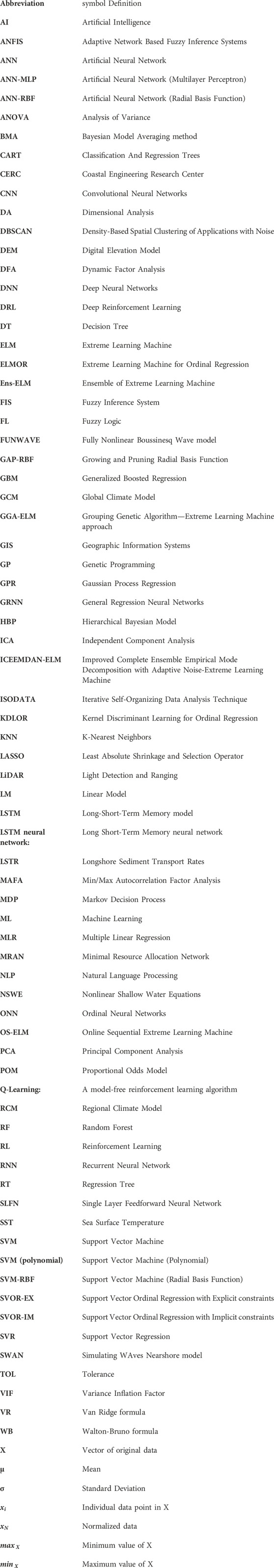
Keywords: machine learning, maritime modelling, classification, prediction, critical review
Citation: Pourzangbar A, Jalali M and Brocchini M (2023) Machine learning application in modelling marine and coastal phenomena: a critical review. Front. Environ. Eng. 2:1235557. doi: 10.3389/fenve.2023.1235557
Received: 06 June 2023; Accepted: 17 August 2023;
Published: 11 September 2023.
Edited by:
Jan Hofman, University of Bath, United KingdomReviewed by:
Soroush Abolfathi, University of Warwick, United KingdomYong Jie Wong, Kyoto University of Advance Science, Japan
Copyright © 2023 Pourzangbar, Jalali and Brocchini. This is an open-access article distributed under the terms of the Creative Commons Attribution License (CC BY). The use, distribution or reproduction in other forums is permitted, provided the original author(s) and the copyright owner(s) are credited and that the original publication in this journal is cited, in accordance with accepted academic practice. No use, distribution or reproduction is permitted which does not comply with these terms.
*Correspondence: Ali Pourzangbar, YWxpLnBvdXJ6YW5nYmFyQGtpdC5lZHU=