Two-decade spatiotemporal variations in ground-level ozone over Ontario, Canada

Introduction: Ground-level ozone (O₃) remains a persistent air quality concern in Ontario, Canada’s most populous province. Understanding long-term trends and spatially explicit details of O₃ is important for supporting air quality management in Ontario.

Method: We construct a high-resolution (daily, 10 km) dataset of maximum daily 8-hour average O₃ (MDA8 O₃) over Ontario from 2004 to 2023, through a two-step machine learning model. The model has incorporated our hypothesis that accounting for transboundary influences can enhance the accuracy of O₃ estimation.

Results: Validation against in-situ measurements confirms the hypothesized high accuracy of the dataset (R² = 0.82, RMSE = 4.99 ppb), outperforming the traditional model and two existing datasets. The dataset reveals pronounced spatiotemporal heterogeneity in MDA8 O₃ concentrations, which are low in northern Ontario but high in southern Ontario, especially in southwest Ontario. Seasonally, the provincial mean MDA8 O₃ peaks in spring (∼40 ppb) and dips in autumn (∼27 ppb), while spatial MDA8 O₃ in summer is most heterogeneous among all seasons, with a peak in southwestern Ontario. From 2004 to 2023, the provincial mean MDA8 O₃ shows no significant trend, while a significant decreasing trend (−0.1 ppb/year, p < 0.05) appears in southern Ontario, where MDA8 O₃ increases in winter but decreases in summer, both significantly. The number of days exceeding the World Health Organization (WHO) O₃ guideline range from 10 to 80 days in southern Ontario, with a decline of 1–4 days (up to 15%) per year over 2004–2023.

Discussion: The analysis suggests that O₃ in southern Ontario is impacted by both anthropogenic emissions and meteorology. Reductions in O₃ precursor emissions have effectively lowered summertime O₃ across southern Ontario, partially offsetting the meteorological-driven increase in O₃. This MDA8 O₃ dataset offers a valuable resource for further research in environmental health, air quality policy, and O₃ impact on agriculture.

1 Introduction

Ground-level ozone (O₃) is a major air pollutant with well-documented adverse effects on human health, ecosystems and agriculture (Fleming et al., 2018; Mills et al., 2018). Although O₃ concentrations in Canada are generally low (WHO, 2023), hourly O₃ concentrations in Ontario (Figure 1), the most populated and urbanized province in Canada, still can be higher than 80 ppb, which is the Ambient Air Quality Criterion (AAQC), particularly in warmer seasons over southern Ontario (Ministry of the Environment and Climate Change, 2022). Continuous monitoring of ground-level O₃ is, therefore, important to supporting air quality management, especially in the populated areas like southern Ontario. The National Air Pollution Surveillance Program (NAPS) has collected hourly ground-level O₃ measurements under a consistent standard protocol since 1969 (https://www.canada.ca/en/environment-climate-change/services/air-pollution/monitoring-networks-data/national-air-pollution-program.html). Based on 39 air monitoring stations in the NAPS program, the Air Quality in Ontario Report show that O₃ pollution during the warm seasons is still an important environmental issue in southwestern Ontario (Ministry of the Environment and Climate Change, 2018a; Ministry of the Environment and Climate Change, 2018b; Ministry of the Environment and Climate Change, 2018c; Ministry of the Environment and Climate Change, 2019; Ministry of the Environment and Climate Change, 2020; Ministry of the Environment and Climate Change, 2021; Ministry of the Environment and Climate Change, 2022). However, the limited numbers and sparsely distribution of monitoring stations across Ontario can introduce substantial geographical bias, restricting the ability to analyze detailed spatial and temporal patterns of ozone (Schultz et al., 2017). As a result, comprehensive assessments of O₃ variability and long-term trends across the province remain limited. In addition, data from sparsely distributed monitoring stations cannot satisfy requirements for studying impact of O₃ pollution on crop yields and O₃-health implications, because spatially explicit and seamless data over large areas are generally needed for these studies.

Figure 1

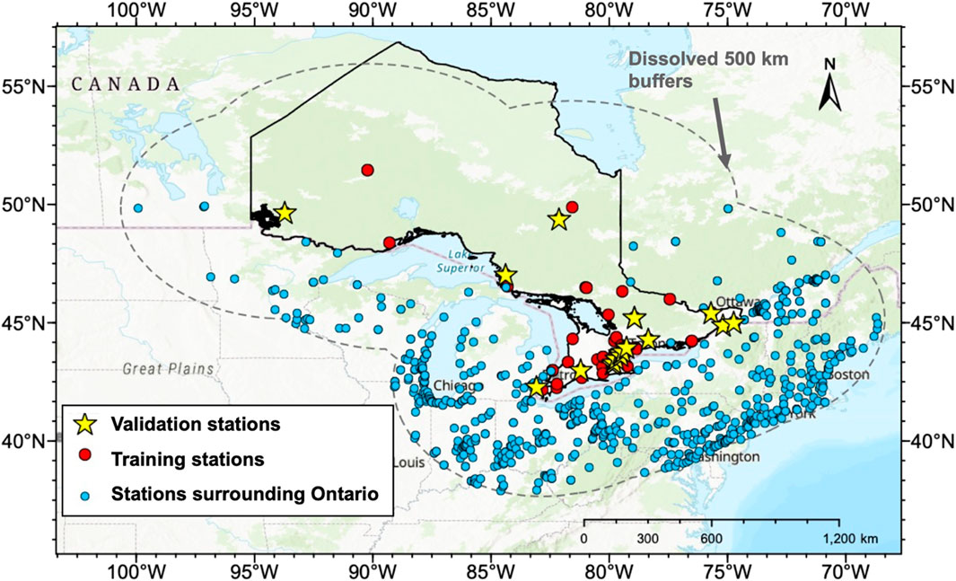
Figure 1. Study area and stations used in this study. The solid black line encloses Ontario province. The gray dashed outline defines the surrounding area of Ontario for the two-step model, which is the dissolved 500 km buffers of each station in Ontario. The star signs indicate the stations for validation, and red dots the stations for training within Ontario. The blue dots indicate the stations surrounding Ontario (within the dashed outline), the data from which are used for the first estimation of O₃ in Ontario by the two-step model.

To address this research gap, it is highly desirable to construct a spatially explicit and long-term dataset of ground-level O₃. However, existing ground-level O₃ datasets for Ontario are confined by their large uncertainties, limited spatial resolution or temporal coverage. While satellite remote sensing has been widely used for air quality monitoring, current retrieval techniques typically provide the total column ozone, tropospheric ozone, or vertical ozone profiles at different vertical ranges (Liu et al., 2010), which do not directly correspond to the ground-level concentrations (Bai et al., 2016). Because ground-level O₃ represents only a small fraction of total column ozone, retrievals based on ultraviolet measurements often have large uncertainties due to limited sensitivity near the ground (Bhartia, 2002). Moreover, satellite records are often short in duration and vary across instruments, and merging these datasets can introduce additional uncertainties (Rahpoe et al., 2015). Chemical transport models (CTMs) can simulate long-term and spatially explicit O₃ fields, but they are also subject to limitations. Notably, large uncertainties remain in simulating O₃ responses to nitrogen oxides (NO_x) emissions, leading to mismatches in magnitude and trends when compared to observations (Miyazaki et al., 2020). Additionally, the spatial resolutions of most CTMs are comparatively coarse (typically >0.5°), which limits their utility for exposure assessments on local and regional scales, especially for health and agriculture applications. To improve the accuracy and spatiotemporal continuity of O₃, statistical models are also widely applied based on the relationship between O₃ and the environmental factors as well as the sources of the precursor emissions. However, to date, a long-term O₃ dataset with fine spatiotemporal resolutions based on statistical models are still unavailable for Ontario. Several studies have provided the global estimations which covers Ontario (Delang et al., 2021; Liu et al., 2023; Wang et al., 2025). However, these datasets are either covering too short periods (<5 years) or with too coarse temporal resolutions (monthly or yearly).

In recent years, machine learning techniques have become preferred statistical algorithms for capturing the nonlinear relationship between O₃ and various factors at regional and global scales (Zang et al., 2021; Chen et al., 2023; Yan et al., 2023). However, machine learning models rely heavily on the density and distributions of in-situ observation stations. In regions distant from any in-situ stations, model predictions could exhibit large modelling errors (Li et al., 2021; Wang et al., 2021). To address this issue, some models, such as linear mixed model (Lee et al., 2011) and geographically weighted regression (Ma et al., 2014), have been used to account for spatial heterogeneity in modelling relationships. However, these models usually assume a linear relationship, limiting their ability at capturing the nonlinear relationships. To overcome this, Li et al. (2021) proposed a locally weighted neural network constrained by global training. However, this approach may face challenges when only short-term in-situ measurements are available, as building a robust global model is difficult. They suggested leveraging data from other regions or time periods to enhance the model robustness. Similar to this idea, Yan et al. (2024) used latent information in grid cells without corresponding in-situ stations to improve the modelling performance over regions with sparse in-situ stations. Despite being effective, the computational cost for those statistical models can become unaffordable when the models are applied at fine resolutions. Liu et al. (2022) incorporated the co-located PM₁₀ stations to enhance the spatiotemporal representativeness and accuracy of PM_2.5 estimations, compromising between leveraging additional information and maintaining computational efficiency.

Here to enable investigation of spatiotemporal variations of O₃ across Ontario, in the first step, we construct a ground-level O₃ dataset over Ontario for two decades (2004–2023) with high accuracy. We select the “maximum daily 8-h average O₃ (MDA8 O₃)” for this dataset because this is one of the metrics that the World Health Organization (WHO) defines to assess air quality impact on health. To this end, we develop a new statistical model for MDA8 O₃ estimation using machine learning techniques. Technically, we use the in-situ stations inside and surrounding Ontario, as well as the data of adjacent grids and time windows from gridded data in our statistical model to fully exploit the information. We validate this dataset with in-situ measurements and compare this dataset with the one from traditional modelling, as well as the existing MDA8 O₃ datasets over Ontario. In the second step, based on the constructed MDA8 O₃ dataset, we analyze the spatial and temporal variations of MDA8 O₃ concentrations across Ontario, showing the trends in response to the meteorological conditions and emission controls over the past two decades. We also assess the O₃ pollution in Ontario following the WHO air quality guidelines. We expect to reveal the spatially explicit seasonality and trend in MDA8 O₃ across Ontario with more details than station data. The developed two-step model provides a novel approach for air pollution modelling, and the MDA8 O₃ dataset can support investigating health and agricultural implications of air quality in the future.

In proximity of the United States of America (USA), air quality in Ontario has been found to be largely influenced by transboundary transport of PM, O₃, and other pollutants from USA (Brook et al., 2002; Johnson et al., 2007; Liu and Cui, 2014; Ministry of the Environment and Climate Change, 2018b). Inspired by previous studies on air quality in Ontario and statistical model development, we make a hypothesis that employing the O₃ data from stations surrounding Ontario in eastern USA, the transboundary influences from eastern USA on surface O₃ in Ontario can be considered and the modelling accuracy can be enhanced. Specifically, we take advantage of the dense O₃ in-situ monitoring stations in Ontario and surrounding areas in the USA to construct a surface MDA8 O₃ dataset over Ontario at daily temporal resolution and 0.1° horizontal resolution.

2 Materials and methods

2.1 Input data

Table 1 shows the input data for constructing the MDA8 O₃ dataset. The in-situ measurements are processed into daily MDA8 O₃ concentrations, in unit of ppb. To unify the spatiotemporal resolution, all the gridded input data are resampled into the spatial resolution of 0.1° (∼10 km), and all the hourly data are averaged into the daily mean.

Table 1

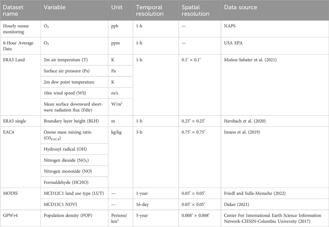
Table 1. Data used for constructing the MDA8 O₃ dataset in this study.

2.1.1 In-situ measurement

The in-situ O₃ measurements over Canada and USA are used for the model development and evaluation. For Canada, hourly in-situ O₃ measurements during 2004–2023 are acquired from the Environment and Climate Change Canada Data (ECCC) Catalogue, provided by the NAPS Program (https://data-donnees.az.ec.gc.ca/data/air/monitor/national-air-pollution-surveillance-naps-program/Data-Donnees/). In addition, 8-h average in-situ ozone data during 2004–2023 are acquired from United States Environmental Protection Agency (EPA) (https://aqs.epa.gov/aqsweb/airdata/download_files.html). The in-situ ozone data are processed into MDA8 O₃ concentrations for every station, according to the Ozone National Ambient Air Quality Standards (NAAQS, https://www.epa.gov/criteria-air-pollutants/naaqs-table).

2.1.2 Reanalysis ozone and precursor data

Reanalysis data benefit the ozone modelling because they combine both model- and observation-based information to provide physically consistent data with continuous spatial and temporal coverage. Here, the surface ozone concentrations from three reanalysis datasets are evaluated: the European Centre for Medium-Range Weather Forecasts (ECMWF) reanalysis version 5 (ERA5), the Modern-Era Retrospective analysis for Research and Applications, Version 2 (MERRA-2), and ECMWF Atmospheric Composition Reanalysis 4 (EAC4). All three reanalysis datasets are processed into the daily mean with 0.1° spatial resolution to compare with in-situ ozone measurements. Figure 2 shows that EAC4 O₃ has the best agreement with in-situ data, with a coefficient of determination (R²) of 0.53 and a root-mean-square error (RMSE) of 29.54 ppb. MERRA-2 performs secondarily (R² = 0.23, RMSE = 34.77 ppb), while ERA5 is with the lowest accuracy (R² = 0.02, RMSE = 44.50 ppb). This is because only EAC4 data include a chemical transport model and consider chemical production and loss of tropospheric O₃ (Vieira et al., 2023), which better captures tropospheric chemistry and ozone dynamics. Therefore, the most accurate EAC4 O₃ data are employed in this study. In addition, O₃ precursors, including HCHO, hydroxyl radical, nitrogen dioxide and nitrogen monoxide from EAC4 are also used to improve the modelling accuracy.

Figure 2

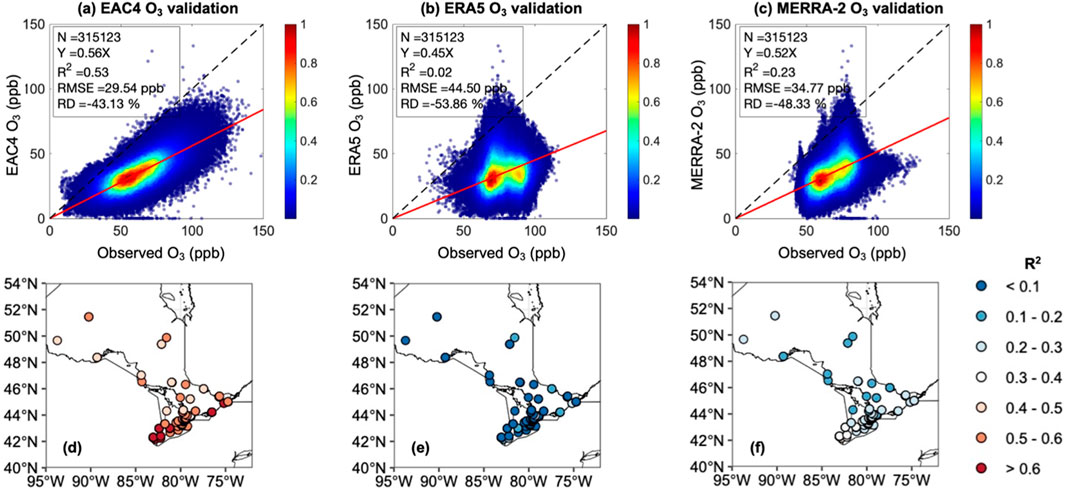
Figure 2. (a) Comparisons of the daily mean surface O₃ between EAC4 and in-situ observations. The black dashed line is the 1:1 line, and the red line is the linear fitting line (with the intercept set to 0). The number of matched samples (N), linear fitting line formula, coefficient of determination (R²), root-mean-square error (RMSE, in ppb) and relative difference [RD, RD = 100 × (estimated O₃ - observed O₃)/(observed O₃), in %] are shown. The color bar represents the density of scatters. (b) same as (a) but for ERA5 O₃. (c) same as (a) but for MERRA-2 O₃. (d) The R² between the daily mean EAC4 O₃ and daily mean in-situ observed O₃ at each station in Ontario. (e) same as (d) but for ERA5 O₃. (f) same as (d) but for MERRA-2 O₃.

2.1.3 Meteorological data

The formation and life span of surface O₃ are closely related to meteorological variables such as solar radiation, temperature, humidity, surface pressure, wind speed and boundary layer height (Agudelo-Castaneda et al., 2014; Khiem et al., 2010; Shen and Mickley, 2017; Hanes et al., 2019). Therefore, these six meteorological variables from ERA5-land are used to enhance the modelling accuracy (Table 1). The high spatial (0.1°) resolution of ERA5 land data also help constrain the spatial resolution of O₃ estimations (Muñoz-Sabater et al., 2021).

2.1.4 Ancillary data

Vegetation and land cover are effective for improving the modelling accuracy, due to their significant association with the spatial distribution of O₃ (Wei et al., 2021; Zang et al., 2021). Here, ancillary inputs are considered including the normalized differential vegetation index (NDVI) and land use from the moderate resolution imaging spectroradiometer (MODIS), and population density from the Gridded Population of World Version 4 (GPWv4).

2.2 The two-step modelling

To fully take advantage of the in-situ measurements surrounding Ontario, a two-step model is developed to build the spatiotemporal relationship between in-situ MDA8 O₃ and multi-source predictors. In step 1, the in-situ measurements surrounding Ontario is used to provide an initial estimation for Ontario MDA8 O₃. In step 2, the initial estimation is combined with in-situ measurements within Ontario to provide a final estimation of spatial-resolved MDA8 O₃ data across Ontario. In addition, the data from the adjacent grid points (8 grids) and time windows (±1 day) for each grid are used in both steps of modelling to fully exploit the information from gridded data. Only the most adjacent grid and time windows are selected here to ensure an acceptable computational time. Both steps use Light Gradient-Boosting Machine (LightGBM) algorithm to build the model, owing to its faster computation speed, lower memory consumption and capability of handling big data (Wei et al., 2021).

Figure 3a shows a detailed framework of this two-step modelling. In step 1, the data from the stations surrounding Ontario (blue stations in Figure 1) are used to provide a reliable estimated Ontario MDA8 O₃ as a new predictor for step 2. To define the surrounding stations, a buffer of 500 km is generated for each station in Ontario (the gray dashed circle in Figure 1). Here, the 500 km buffer is determined by the most conservative ozone correlation length (500–1,000 km) in the troposphere, within which ozone concentrations are considered being significantly correlated (Liu et al., 2009). Therefore, for each station in Ontario, the stations within the radius of 500 km outside Ontario can be determined as its surrounding stations. By merging all the radius of 500 km for each station in Ontario, the stations outside Ontario but within this buffer are considered as the surrounding stations. Step 2 is similar to traditional modelling (Figure 3b), yet with an additional predictor from the estimated MDA8 O₃ from step 1. In this way, the uncertainty of the modelling is further reduced and the final estimation of MDA8 O₃ is achieved. Compared to traditional models, the two-step model is trained not only with Ontario data but also with data in nearby regions, which captures broader regional patterns and long-range transport that influence O₃ in Ontario, especially in border areas.

Figure 3

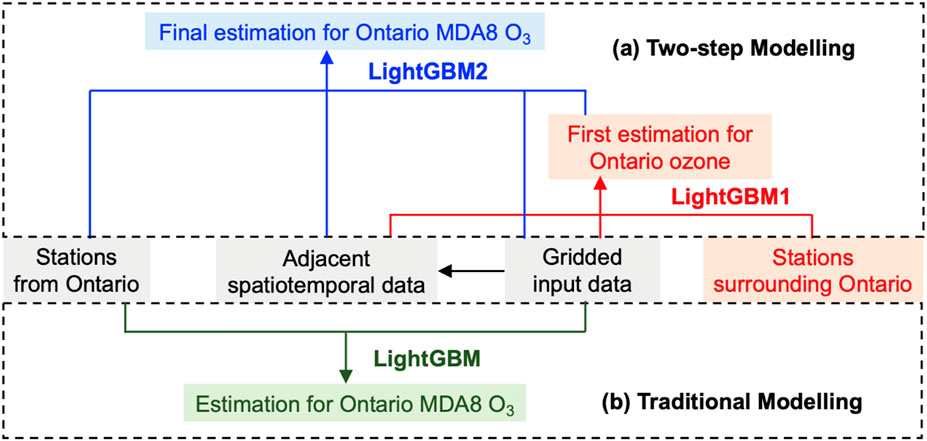
Figure 3. Flowchart of the two-step modelling developed in this study (a) and traditional modelling (b) Note that LightGBM1 and LightGBM2 indicate two different models are trained based on LightGBM algorithm.

Specifically, step 1 is formulated as Equation 1:

$O_{3\_surrouding}=f_1\left(T,Ps,RH,WS,Fdir,BLH,{\mathrm{O}}_{3\text{EAC}4},\text{OH},{\text{NO}}_2,\text{NO},\text{HCHO},\text{LUT},\text{NDVI},\text{POP}\right)(1)$

where $O_{3\_surrouding}$ represents the MDA8 O₃ estimation from stations surrounding Ontario, and $f_1$ denotes the LighGBM1 model illustrated in Figure 2a. All predictor variables are listed in Table 1. Using the trained $f_1$, the MDA8 O₃ is estimated at each station and grid in Ontario, i.e., $O_{3_{f1}}$.

Step 2 integrates this initial estimate ($O_{3_{f1}}$) to predict the final O₃ in Ontario as Equation 2:

$O_{3\_ontario}=f_2\left(O_{3_{f1}},T,Ps,RH,WS,Fdir,BLH,{\mathrm{O}}_{3\text{EAC}4},\text{OH},{\text{NO}}_2,\text{NO},\text{HCHO},\text{LUT},\text{NDVI},\text{POP}\right)(2)$

where $O_{3\_ontario}$ represents the MDA8 O₃ measurements from stations surrounding Ontario, and $f_2$ represents the LighGBM2 (Figure 2a). Except for including $O_{3_{f1}}$, the remaining variables used in step 2 are the same as (1) and listed in Table 1.

2.3 Validation and comparison

To validate the modelling accuracy, different training and validation datasets are selected. For step 1, the surface MDA8 O₃ from the surrounding stations and the data from Ontario stations are used for model training and validation, respectively. For step 2, the data are randomly divided into 10 groups based on the stations, i.e., data samples from the same station will not be split. This way of data split is considered the most reliable for validating spatial extrapolation (Li et al., 2020). Eight groups of data are used for model training, and the rest two groups for validation. Figure 1 shows the stations selected for model training (red points) and validation (star signs) in step 2.

In addition, the estimated MDA8 O₃ by the two-step model is also compared with two published datasets on the global scale, as no gridded MDA8 O₃ datasets specifically for Ontario. These two datasets include the daily MDA8 O₃ data from 2019 to 2021 produced by Wang et al. (2025) and the annual O₃ from 2004 to 2017 produced by Delang et al. (2021). The comparisons of MDA8 O₃ estimations are based on their agreements with all the in-situ MDA8 O₃ measurements in Ontario.

2.4 Removing meteorological impacts

To quantify the non-meteorological impacts on O₃ trends, primarily those associated with anthropogenic activities, meteorological-adjusted O₃ trends are derived. Meteorological impacts are removed using a multiple linear regression model, as Equation 3 following previous studies (Tai et al., 2010; Yang et al., 2019):

$C\left(t\right)={\displaystyle \sum _{i=1}^n}{a}_i{V}_{i(t)}+b+r_{(t)}(3)$

where $C\left(t\right)$ represents the daily MDA8 O₃ from 2004 to 2023 obtained by two-step model; n is the number of meteorological variables, including all the inputs for the two-step model (Fdir, T, RH, WS and Ps,); i is an index for the meteorological variables. $V_{i(t)}$ is the daily meteorological variable i from 2004 to 2023; $a_i$ and $b$ are the regression coefficient for meteorological variable i and the intercept of regression; $r_{(t)}$ is the residual term, which represents the MDA8 O₃ after removing the meteorological impact (i.e., met-adjusted MDA8 O₃).

3 Results

3.1 Accuracy of the estimated surface O₃ concentrations

Figure 4a shows the validation of the estimated MDA8 O₃ by the two-step model against the in-situ measured MDA8 O₃. By station-based validation, the overall agreement is well, with R² of 0.83 and RMSE of 4.99 ppb. For each step in the modelling, the initial estimation of MDA8 O₃ using surrounding stations achieves an accuracy of R² being 0.74 and RMSE being 6.05 ppb, and the final estimation further increases the R² by 12% and decreases the RMSE by 21%. Compared to traditional modelling (Figure 4b), on average, the two-step modelling increases R² by 10% and decreases RMSE by 16%, indicating the advantages of considering surrounding stations and incorporating spatial and temporal dependencies. In addition, the two-step modelling has improved the R and RMSE from the traditional modelling, quantified as [100 × (two-step modelling - traditional modelling)/traditional modelling] for both R² and RMSE. Spatially, Figures 4c,d show that R² is increased to >15% and RMSE is decreased to <25%. The improvement is the higher in the south than in the north, likely because most of the surrounding stations are located around southern Ontario.

Figure 4

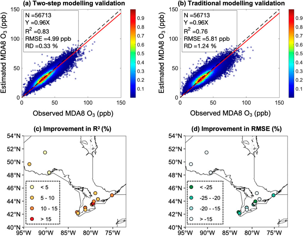
Figure 4. (a) Comparisons of the two-step model estimated daily MDA8 O₃ against daily in-situ observed MDA8 O₃. The black line is the 1:1 line, and the red line is the linear fitting line (with the intercept set to 0). The number of matched samples (N), linear fitting line formula, coefficient of determination (R²), root-mean-square error (RMSE, in ppb) and relative difference [RD, RD = 100 × (estimated MDA8 O₃ - observed MDA8 O₃)/(observed MDA8 O₃), in %] are shown. The color bar represents the density of scatters. (b) same as (a) but for traditional model estimated daily MDA8 O₃. (c) The improvement of R² between the two-step modelling and traditional modelling (in %), calculated as 100 × (R² of two-step modelling - R² of traditional modelling)/R² of traditional modelling. (d) same as (c) but for RMSE.

The improved accuracy is especially important for better capturing O₃ concentrations on polluted days. Figure 5 shows the MDA8 O₃ concentrations over southern Ontario on 20 July 2021, when high levels of air pollution were reported due to the wildfire smoke (https://ottawa.citynews.ca/2021/07/20/special-air-quality-advisory-issued-for-southern-ontario-due-to-wildfire-smoke-3969377/?utm_source=chatgpt.com). Figures 5a,b show the extremely high O₃ concentrations from both models estimated (the base map) and in-situ observed (circles) results. However, traditional modelling underestimates the high MDA8 O₃ concentrations over southeastern Ontario, as well as over the coastal area of southwestern Ontario. Figures 5b,c quantify that traditional modelling underestimates the MDA8 O₃ concentrations by a relative difference (RD) of 7%, while the two-step modelling has a good agreement with observation, indicated by an improved RD of 0.3%.

Figure 5

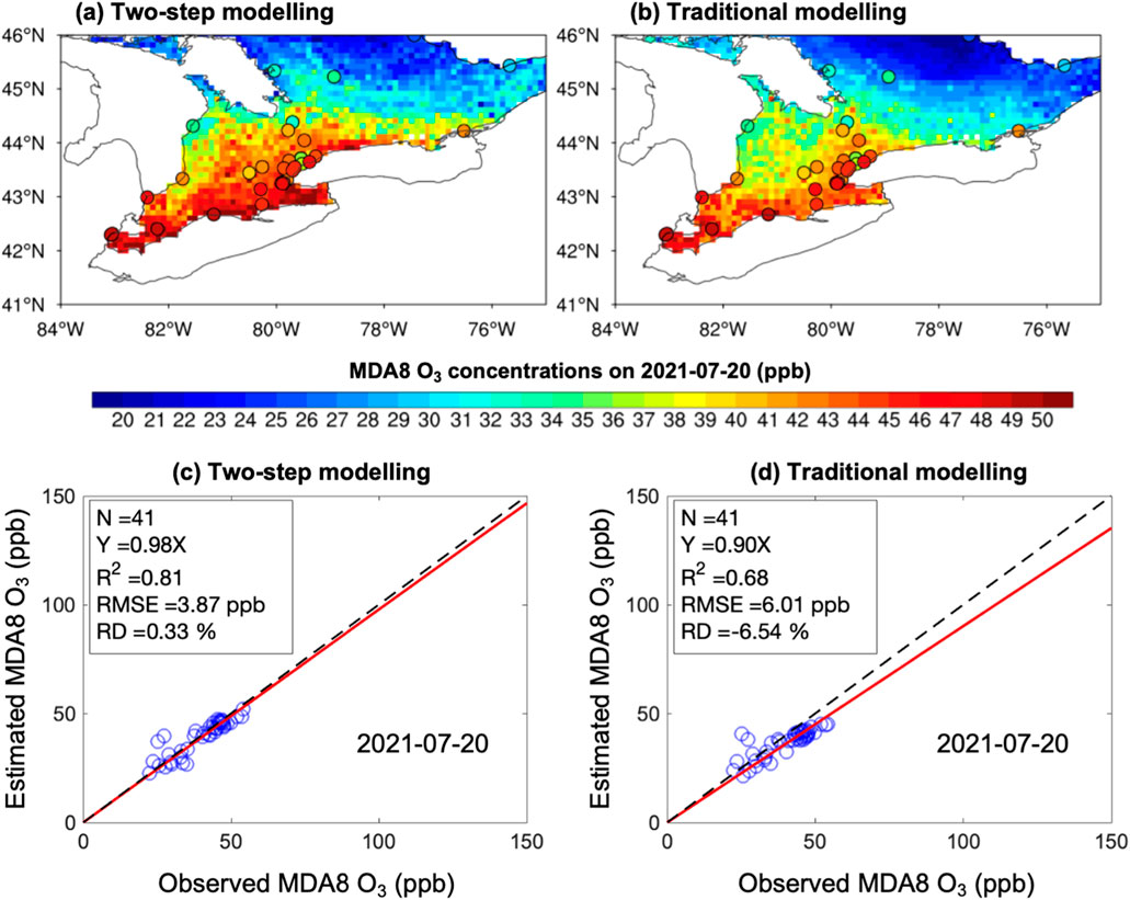
Figure 5. (a) The MDA8 O₃ spatial distribution from the two-step modelling estimation (the base map) and in-situ observation (the circles) on 20 July 2021. (b) same as (a) but from the traditional modelling estimation. (c) Comparisons of daily MDA8 O₃ between the two-step model estimations and in-situ observations on 20 July 2021. The black line is the 1:1 line, and the red line is the linear fitting line (with the intercept set to 0). The number of matched samples (N), linear fitting line formula, coefficient of determination (R²), root-mean-square error (RMSE, in ppb) and relative difference [RD, RD = 100 × (estimated MDA8 O₃ - observed MDA8 O₃)/(observed MDA8 O₃), in %] are shown. (d) same as (c) but for traditional model estimation.

Figure 6 compares the estimated MDA8 O₃ using the two-step model with two published MDA8 O₃ datasets. Note that these two datasets are aimed at offering MDA8 O₃ concentrations globally, rather than specifically for Ontario. All the data from in-situ MDA8 O₃ monitoring stations over Ontario are used to compare the accuracy of the three MDA8 O₃ datasets. Compared to the daily MDA8 O₃ dataset over 2019–2021 from Wang et al. (2025) (Figure 6b), the two-step model (Figure 6a) enhances the R² by 11% and reduces RMSE by 24% and RD by 58%. In a longer period over 2004–2017, the estimated yearly MDA8 O₃ concentrations (Figure 6c) are compared with those from Delang et al. (2021) (Figure 6d). The two-step model estimated MDA8 O₃ shows a better agreement with the in-situ O₃, with R² higher by 0.3 and RMSE lower by 5.5 ppb. Also, a clear overestimation of MDA8 O₃ is apparent in Delang et al. (2021) with RD of 17%, while the RD in our dataset is only about 0.2%.

Figure 6

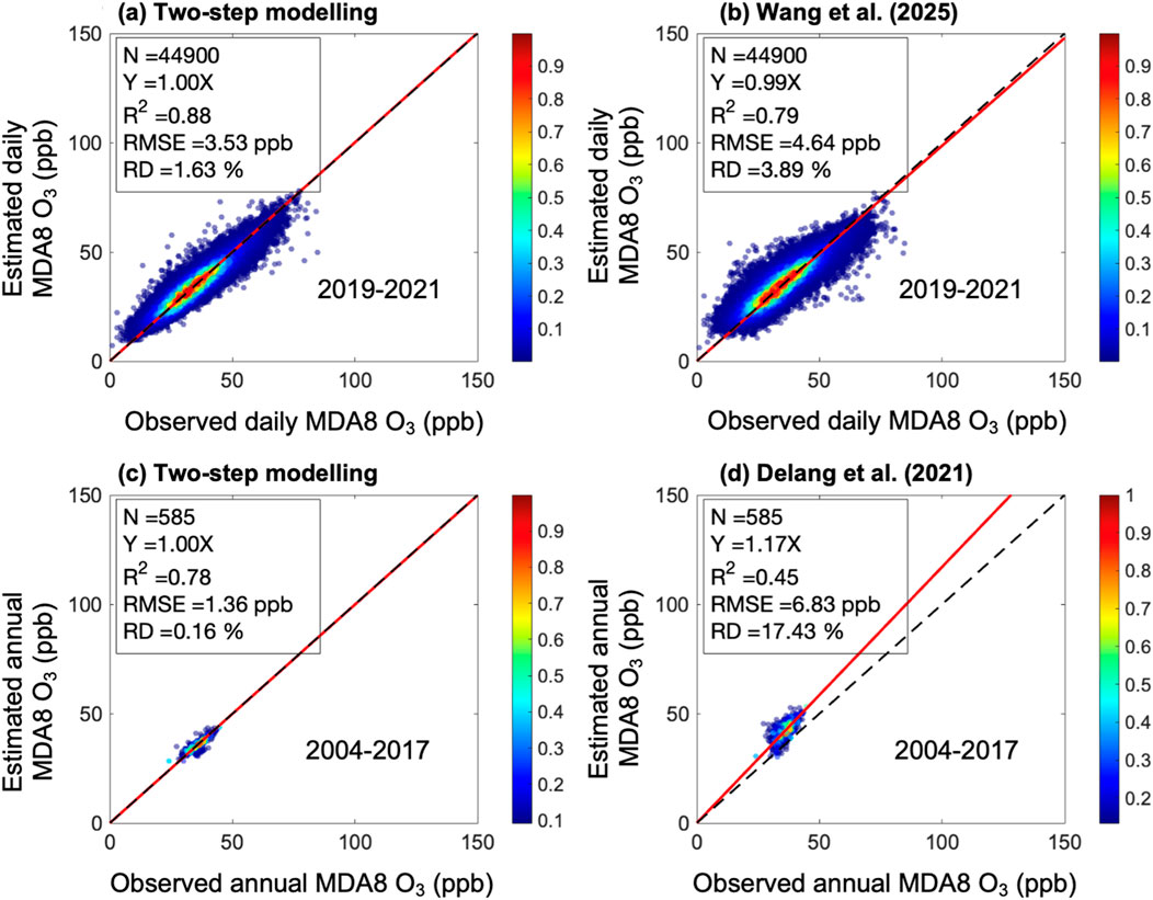
Figure 6. (a) Comparisons of in-situ daily MDA8 O₃ observations during 2019–2021 against the two-step model estimations. (b) same as (a) but against the MDA8 O₃ estimation by Wang et al. (2025). (c) Comparisons of the in-situ annual mean MDA8 O₃ observation during 2004–2017 against the two-step model estimations. (d) same as (c) but against the MDA8 O₃ estimation by Delang et al. (2021). The black line is the 1:1 line, and the red line is the linear fitting line (with the intercept set to 0). The number of matched samples (N), linear fitting line formula, coefficient of determination (R²), root-mean-square error (RMSE, in ppb) and relative difference [RD, RD = 100 × (estimated MDA8 O₃ - observed MDA8 O₃)/(observed MDA8 O₃), in %] are shown. The color bar represents the density of scatters.

3.2 Spatial variations of surface O₃ concentrations over Ontario

Based on the daily MDA8 O₃ concentrations estimated by the two-step model, the spatial variations of O₃ over Ontario from 2004 to 2023 are studied. Figure 7 shows the 20-year mean daily MDA8 O₃ over Ontario, capturing the high values over southern Ontario. In general, Table 2a shows that the mean concentrations of daily MDA8 O₃ over southern Ontario (36.83 ± 9.82 ppb) is about 4 ppb higher than over Ontario (32.94 ± 8.21 ppb). Compared to the north, southern Ontario is more densely populated and urbanized, with the western edge close to the major populated industrial cities such as Detroit and Windsor (Figure 7b). Therefore, the high MDA8 O₃ concentrations over southern Ontario are largely attributed to industrial emissions of O₃ precursors such as nitrogen oxides and sulfur oxides (McGuire et al., 2011; Halla et al., 2011). Owing to the high spatial resolution (10 km) of this dataset, the regional difference is also observed among southern Ontario. In Toronto city, due to the higher rate of ozone depletion by traffic-emitted NO_x (Geddes et al., 2009; Huryn and Gough, 2014), the O₃ concentrations (30–32 ppb) are lower than the concentrations (>35 ppb) over southwestern Ontario (Figure 7b). In addition, the transported O₃ and precursor by southwesterly airflows from USA contribute to the higher O₃ concentrations over southwestern Ontario than Toronto city as well (Makar et al., 2010; Ministry of the Environment and Climate Change, 2018c). At regions near lakeshore over southern Ontario, Figure 6a shows lower MDA8 O₃ concentrations than inland, indicating the influence of land-lake breeze that dilutes the O₃ concentrations near lake and results in an O₃ gradient at the lake edge (Huang and Donaldson, 2024).

Figure 7

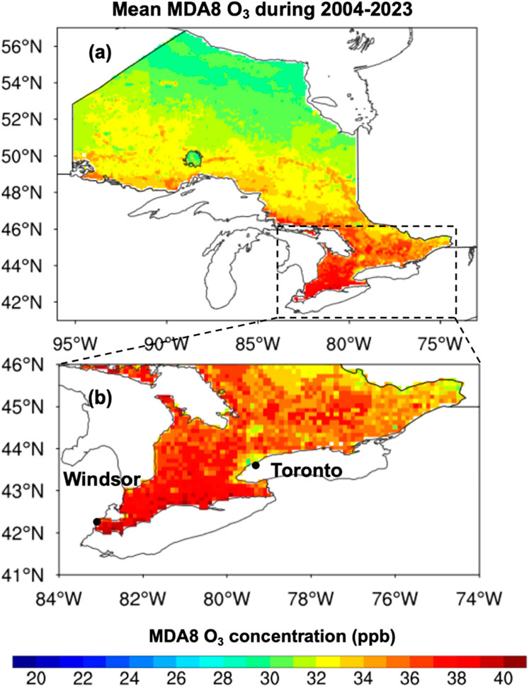
Figure 7. (a) The spatial distribution of the mean MDA8 O₃ (in ppb) over Ontario during 2004–2023. (b) Same as (a) but for southern Ontario (up to 46°N). The mean MDA8 O₃ concentrations over Ontario and southern Ontario are shown in Table 2a. The two dots indicate the locations of Toronto and Windsor.

Table 2

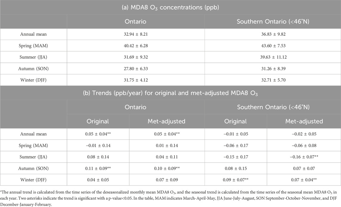
Table 2. (a) The annual and seasonal mean MDA8 O₃ concentrations ± standard deviations averaged over Ontario and southern Ontario during 2004–2023 (in ppb). (b) The annual and seasonal MDA8 O₃ trends ±95% confidence interval for Ontario and southern Ontario during 2004–2023 (in ppb/year)^a.

3.3 Temporal variations of surface O₃ concentrations over Ontario

3.3.1 Seasonal variation

Seasonality greatly modulates the magnitude of daily MDA8 O₃ concentrations in Ontario (Leung et al., 2021). For both Ontario and southern Ontario (Table 2a), MDA8 O₃ concentrations during warm seasons (spring and summer) are higher than the ones during cold seasons (autumn and winter), due to the more active photochemical O₃ formation under higher temperature and solar radiation (Crutzen, 1974), as well as the strongest stratospheric intrusions in spring (Monks, 2000). Figures 8a–d show the spatial distributions of MDA8 O₃ over southern Ontario in each season. High MDA8 O₃ concentrations are more homogeneously in spring than in summer when MDA8 O₃ hotspots are concentrated over the western region (Figure 8a vs; Figure 8b), which is also reflected in the overall higher MDA8 O₃ concentrations in spring than in summer (Table 2a). Such spatial inhomogeneity in summer continues in autumn but subsides in winter when MDA8 O₃ concentrations become homogeneously low over entire southern Ontario (Figure 8c vs; Figure 8d).

Figure 8

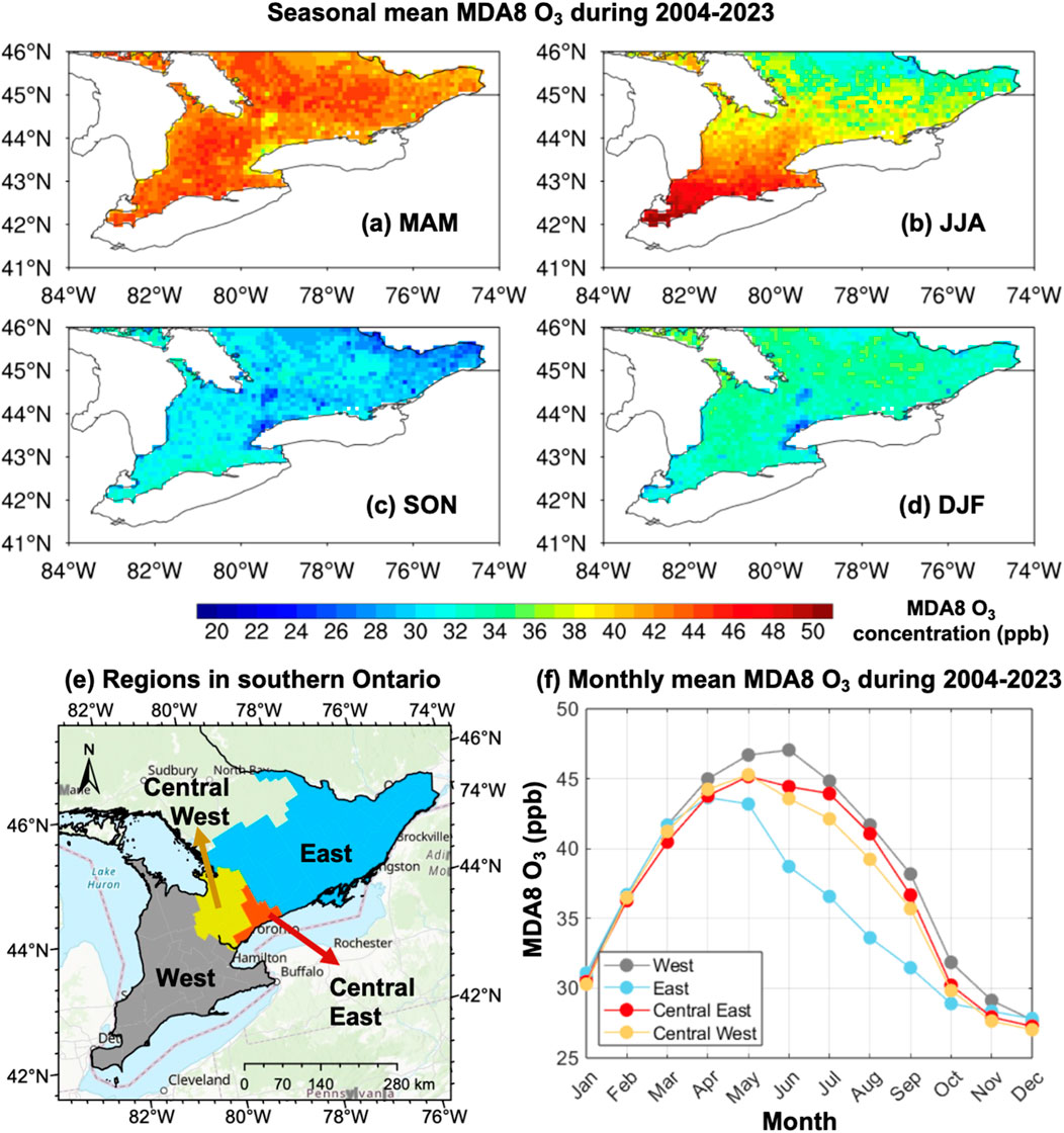
Figure 8. (a–d) The spatial distribution of the mean MDA8 O₃ (in ppb) over southern Ontario (42–46°N) during 2004–2023 by season: MAM (March-April-May), JJA (June-July-August), SON (September-October-November) and DJF (December-January-February). The mean MDA8 O₃ concentrations over southern Ontario are shown in Table 2a. (e) The sub-regions (the west, central west, central east and east) in southern Ontario indicated by colors and (f) the corresponding seasonal variations in MDA8 O₃ for the four regions, based on the 20-year monthly mean.

Figure 8f further shows the 20-year mean MDA8 O₃ in each month over four subregions of southern Ontario: the west, central west, central east and east regions (Figure 8e). Among the four subregions, O₃ concentrations in the west is the highest throughout the year with a clear peak (47.06 ppb) in June. In contrast, the east shows the lowest MDA8 O₃ concentrations during April-October among all the subregions, with a peak (43.66 ppb) in April. Both central west (45.28 ppb) and central east (45.16 ppb) show a peak in May, with intermediate MDA8 O₃ concentrations between the west and east. The spring O₃ maximum is widely found over the midlatitudes of Northern Hemisphere (Monks, 2000; Gaudel et al., 2018), which are attributed to the enhanced photochemistry in spring after the accumulation of O₃ precursor in winter (Penkett and Brice, 1986), as well as stratospheric intrusions (Monks, 2000). However, in summer, high MDA8 O₃ concentrations still prevail over southwestern Ontario, with much higher values than in the other seasons. The summer O₃ maximum is typical for regions dominated by anthropogenic photochemical ozone production and long-range transport (Singh et al., 1967; Logan, 1985). Due to being closer to industrial regions and being influenced by O₃ transported by southwesterly wind, southwestern Ontario shows a summer peak in O₃. The different seasonal peaks between southeastern and southwestern Ontario indicate different sources of O₃ over southern Ontario.

3.3.2 Long-term trend

The constructed dataset covers 20 years from 2004 to 2023, enabling investigation of the MDA8 O₃ trend during the 20 years over Ontario, especially over southern Ontario where O₃ pollution is severest in the province. Table 2b summarizes the MDA8 O₃ trends during 2004–2023 for the entire Ontario and southern Ontario, respectively. Over the entire Ontario, a significant (p < 0.05) increase of 0.05 ± 0.04 ppb/year is observed. In contrast, southern Ontario exhibits a non-significant (p > 0.05) trend of −0.01 ± 0.05 ppb/year, which agrees with the no clear O₃ trends in the recent 10 years documented the Air Quality in Ontario Report (Ministry of the Environment and Climate Change, 2018a; Ministry of the Environment and Climate Change, 2018b; Ministry of the Environment and Climate Change, 2018c; Ministry of the Environment and Climate Change, 2019; Ministry of the Environment and Climate Change, 2020; Ministry of the Environment and Climate Change, 2021; Ministry of the Environment and Climate Change, 2022). Because most of the O₃ monitoring stations are located in southern Ontario (Figure 1), the regional discrepancy suggests an increase in MDA8 O₃ in northern Ontario, where monitoring coverage is limited. Despite the overall non-significant trend over southern Ontario, spatial heterogeneity is clear. Figure 9a shows the distributions of the MDA8 O₃ trend for southern Ontario, which reveals a significant (p < 0.05) decreasing trend over southwestern Ontario at a rate about −0.1 ppb/year. However, over southeastern Ontario, the MDA8 O₃ concentrations increase significantly at a rate about 0.1 ppb/year.

Figure 9

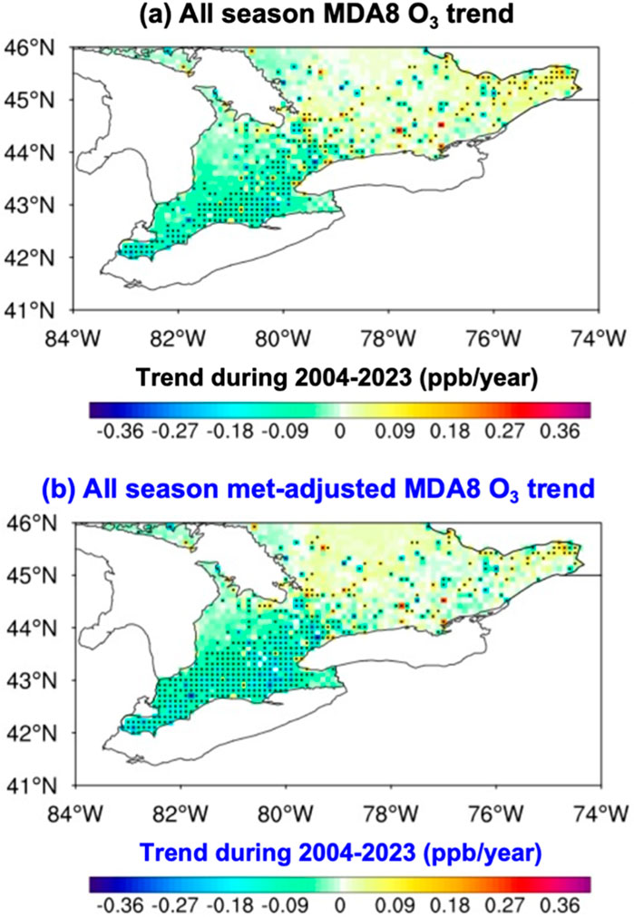
Figure 9. (a) The spatial distribution of MDA8 O₃ trend over southern Ontario during 2004–2023 (in ppb/year). Note that the trend is calculated from the time series of the deseasonalized monthly mean MDA8 O₃. Dotted area indicates trends are significant at the 95% level. (b) same as (a) but for the spatial distribution of met-adjusted trend.

Given the significant influence of meteorological conditions on long-term MDA8 O₃ trends, the meteorological-impact-removed, namely, met-adjusted, MDA8 O₃ trend (see Section 2.4) during 2004–2023 is further analyzed. Table 2b shows that for the entire Ontario, the magnitude of met-adjusted MDA8 O₃ trend remains the same as the original trend (0.05 ± 0.04 ppb/year), indicating that the general trend in Ontario is dominated by non-meteorological drivers. For southern Ontario, compared to the original trend, met-adjusted MDA8 O₃ exhibits a slightly stronger decline (−0.02 ppb/year), and a greater magnitude and a broader area of decrease in southwestern Ontario (Figure 9b). This indicates that non-meteorological drivers, primarily emission reductions, is greater than what is observed from the real MDA8 O₃ trend and the meteorological impact on MDA8 O₃ trend is positive, which partially offsets the impact of the reduction of precursor emissions.

Seasonally, over 2004–2023, distinct difference also shows in trends over the entire Ontario and southern Ontario. For the entire Ontario, both original and met-adjusted MDA8 O₃ trends show significant increases only in autumn with similar magnitudes (about 0.10 ± 0.09 ppb/year), while trends in other seasons are not statistically significant (Table 2b). For southern Ontario, MDA8 O₃ decreases in warm seasons (spring and summer), especially in summer, which is in contrast to its increases in cold seasons (autumn and winter), especially in winter (Figures 10a,b vs; Figures 10c,d). There are larger areas with significant trends in cold seasons than in the warm seasons, with largest areas with increasing trends in winter across southern Ontario. In comparison, warm seasons show the significant decreasing trends only over southwestern Ontario. Correspondingly, in the sub-regions over southern Ontario (Figure 9b), wintertime MDA8 O₃ increases significantly in all the four sub-regions, while summertime MDA8 O₃ decreases significantly only the west (Table 3). The decrease of MDA8 O₃ in spring and increase of MDA8 O₃ in autumn are both not significant in all the four sub-regions (Table 3).

Figure 10

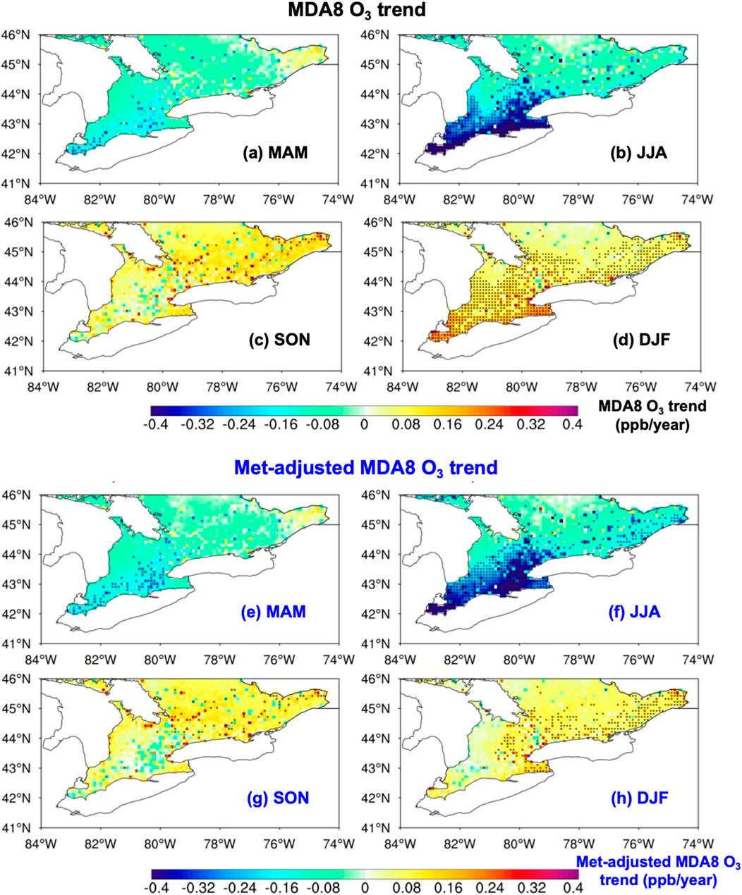
Figure 10. (a–d) The spatial distribution of MDA8 O₃ trend over southern Ontario in each season during 2004–2023 (in ppb/year). Note that the trend is calculated from the time series of the seasonal mean MDA8 O₃ in each year. Dotted area indicates the trends being significant at the 95% level. The mean trend ±95% confidence interval during 2004–2023 is given in Table 2b, calculated by the seasonal mean MDA8 O₃ time series averaged over southern Ontario. (e–h) same as (a–d) but for met-adjusted trend.

Table 3

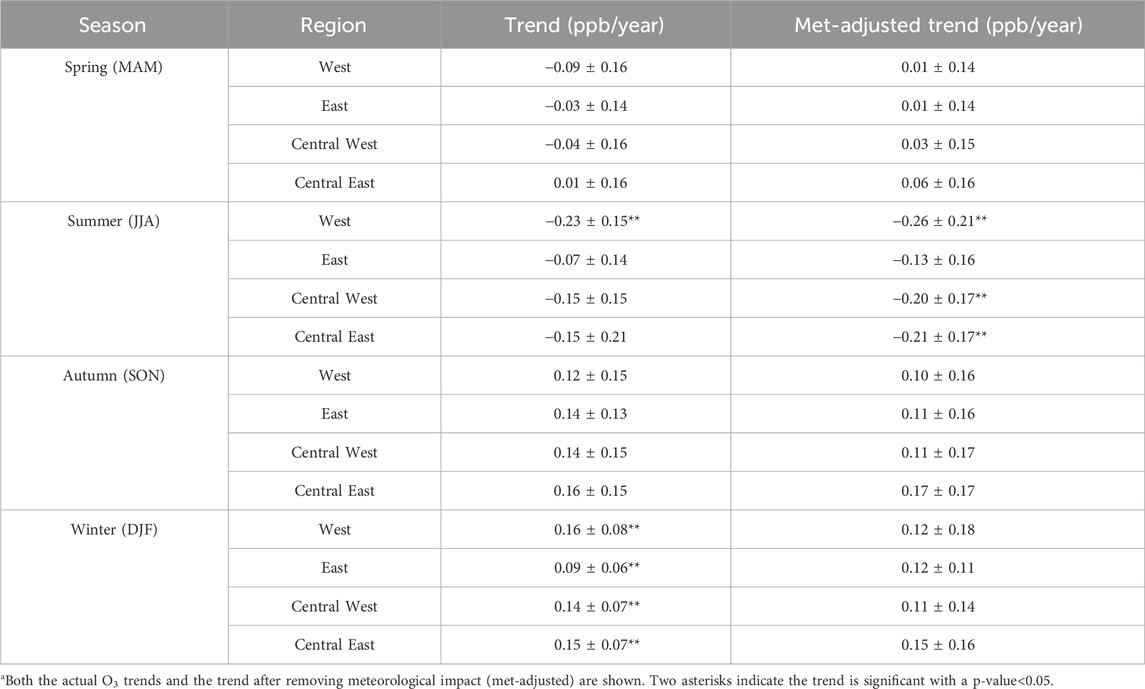
Table 3. The MDA8 O₃ trends ±95% confidence interval by season for the four regions (see Figure 8c) in southern Ontario during 2004–2023 (in ppb/year)^a.

Similar to the annual mean (Figure 9), after removing the meteorological impact, the met-adjusted MDA8 O₃ trend in warm seasons shows a greater decrease with broader areas, particularly in southeastern Ontario (Figures 10e,f). Particularly, the central west and central east regions show significantly decrease in met-adjusted O₃ trend in summer, in contrast to the non-significant actual O₃ trends in those regions (Table 3). The significant decrease in summertime O₃ over southern Ontario is mainly due to the progressive controls of NO_x emissions in Ontario and the USA, which decrease local ozone formation and transboundary influences (Ministry of the Environment and Climate Change, 2018). Despite being offset by meteorological-driven increases in O₃, the actual trend remains negative, significantly with a magnitude larger than 0.2 ppb/year in southeastern Ontario (Figure 10b). In summer, a comparison of the MDA8 O₃ trend in southern Ontario and with that in the entire Ontario (Table 2b) suggests an increasing O₃ trend in northern Ontario.

During cold seasons, MDA8 O₃ increases non-significantly in autumn, but significantly in winter over southern Ontario, especially in southeastern Ontario (Figures 10d,h, Table 2b). The wintertime MDA8 O₃ trends in the four sub-regions of southeastern Ontario all turn from significant increase to non-significant after removing meteorological impacts (Table 3). The increased O₃ during cold seasons is likely to mainly attribute to an increase in the global background O₃ concentrations (Reid et al., 2008; Parrish et al., 2012), which is positively overlaid by the impact of meteorological variability over 2004–2023. In contrast to the non-significant MDA8 O₃ trends in autumn over southern Ontario, the significant increase over the entire Ontario in autumn implies a pronounced increase over northern Ontario (Table 2b). The increasing MDA8 O₃ over northern Ontario during summer and autumn could be driven by wildfire emissions, as it coincides with the wildfire season as well as the increasing wildfire activities, e.g., area burned and number of large fires in Ontario (Hanes et al., 2019; Jain et al., 2024).

3.4 O₃ exceedance days

The 2021 WHO air quality guidelines recommend that the health level of MDA8 O₃ concentrations should be lower than a threshold of 100 μg/m³ or 50 ppb. Thus, a day with MDA8 O₃ concentrations larger than this threshold is referred as the O₃ exceedance day. Based on the constructed daily O₃ dataset, Figure 11a shows the mean exceedance days per year during 2004–2023 at each of the 10-km grids. The number of exceedance days is largest around the most southwestern region, reaching ∼80 days per year. The number decreases gradually northward, with ∼10 days per year in the northern region. Such a spatial pattern resembles O₃ concentrations (Figure 7b), indicating concurrent higher O₃ concentrations and more O₃ exceedance days.

Figure 11

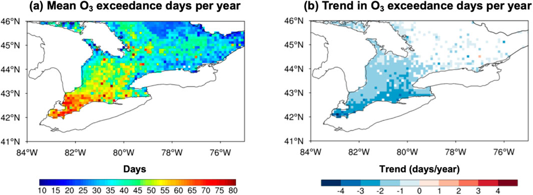
Figure 11. (a) The spatial distribution of the mean O₃ exceedance days per year over southern Ontario during 2004–2023. (b) The trend in O₃ exceedance days per year over southern Ontario during 2004–2023 (in days/year). Note that only the grids with trends that are significant at the 95% level are shown.

Figure 11b shows a significant decreasing trend in the number of O₃ exceedance days, particularly in southwestern Ontario by up to 4 days/year (equivalent to about 15%/year). Differently from the slight increasing trend in O₃ concentrations over southeastern Ontario (Figure 9a), the frequency of high O₃ concentrations is decreasing over the entire southern Ontario. This improvement shows the effective controls of O₃ pollution in Ontario.

4 Discussion and conclusion

To study the long-term and spatially explicit O₃ concentrations and trends over Ontario, we constructed a dataset of daily MDA8 O₃ concentrations with a spatial resolution of 10 km for Ontario. This dataset is constructed based on surface O₃ observations at individual stations from NAPS program and USA EPA (Table 1), using a two-step statistical model built by LightGBM algorithm. The two-step model integrates MDA8 O₃ measurements from neighboring stations within 500 km, along with data from adjacent grid points (8 surrounding grids) and time windows (±1 day), to improve modelling accuracy. Multi-sources input data, including meteorological, satellite and emission data, are used as the predictors (Table 1).

The modelling performance is validated using station-based data to represent spatial predictability. Across validation stations, the two-step model achieves high accuracy, with an R² of 0.82 and a RMSE of 4.99 ppb (Figure 4). Our results are compared with two global MDA8 O₃ datasets from Wang et al. (2025) at daily time step (2019–2021) and from Delang et al. (2021) at annual time step (2004–2017) (Figure 6). Our dataset shows a better agreement with in-situ measurements than both MDA8 O₃ datasets. To test the hypothesis suggested in Introduction, the two-step model is also compared with the traditional model that uses O₃ measurements from stations in Ontario only (Figure 3b). The two-step model improves R² by 10% and reduces RMSE by 16% (Figures 4a,b), with greater improvements in southern Ontario (Figures 4c,d) because of inclusion of O₃ data from the high density of surrounding stations. The two-step model also better captures MDA8 O₃ distributions than the traditional model under heavy pollution conditions (Figure 5).

Based on this long-term and high spatiotemporal-resolution MDA8 O₃ dataset, the spatiotemporal variations of MDA8 O₃ over Ontario are further studied. The spatial distribution captures the higher MDA8 O₃ concentrations over densely populated and urbanized southern Ontario, particularly the southwestern areas that are mostly industrialized and also influenced by the southwesterly transported air pollutants (Figure 7). The seasonal variations reveal the elevated O₃ concentrations during warm seasons compared to cold seasons (Figures 8a–d; Table 2a). Due to the accumulation of O₃ precursors during winter and frequent stratospheric intrusions, southern Ontario exhibits the highest ozone concentrations in spring. During summer, high O₃ levels persist over southwestern Ontario (Figures 8e,f), with peak values in June (Figure 8f), showing largest spatial heterogeneity among all seasons. This summertime O₃ maximum is typical for regions influenced by intense anthropogenic photochemical ozone production and long-range transport (Singh et al., 1967; Logan, 1985). Southwestern Ontario is greatly impacted by both local and transboundary anthropogenic emissions, including those from the industrialized “Chemical Valley” region and its surroundings (MacDonald and Rang, 2007). The ozone precursors such as VOCs in southwestern Ontario (e.g., Hamilton downtown) can reach 39 μg/m³ but only 36 μg/m³ in Toronto (Bari and Kindzierski, 2018). In addition, transport from southwestern Michigan contributes substantially to ozone levels in this region (AQA, 2023).

During 2004–2023, MDA8 O₃ trends show a distinct difference over entire Ontario and southern Ontario. For southern Ontario, there is a non-significant (p > 0.05) decrease of 0.01 ppb/year (Table 2b), consistent with the report by Air Quality in Ontario (Ministry of the Environment and Climate Change, 2016–2022). However, the spatial distribution of MDA8 O₃ trends is heterogeneous, revealing a significant decrease in southwestern Ontario (∼0.1 ppb/year) and an increase in southeastern Ontario (∼0.1 ppb/year) during 2004–2023 (Figure 9a). After removing the meteorological impact, the O₃ trend over southern Ontario shifts to a stronger decrease of −0.02 ppb/year (Table 2b, Figure 9c), suggesting that a meteorological-driven increase in O₃ has partially offset by a decrease in O₃ due to precursor emission reductions. For entire Ontario, both original and met-adjusted MDA8 O₃ increases significantly at a rate about 0.05 ppb/year (Table 2b), indicating that the general trend in Ontario is dominated by non-meteorological drivers.

By season, a significant increase trend occurs during winter across southern Ontario (Figure 10d), likely due to the increase in global background O₃ to some degree (Reid et al., 2008; Parrish et al., 2012). Previous studies have reported increases in the continental or hemispheric background O₃ from measurements at remote stations or through meteorological adjustments (Vingarzan, 2004; Oltmans et al., 2006; Chan, 2009; Chan and Vet, 2010). After removing meteorological influences, the wintertime O₃ trend from 2004 to 2023 becomes statistically non-significant over southern Ontario (Figure 10h; Table 2). This suggests that the positive O₃ trend in winter is largely meteorological-driven. In contrast, O₃ in summer decreases significantly, particularly over southwestern Ontario (Figure 10b). The meteorological-impact-remove trends in summer are more negative in a larger area than the actual trends (Figure 10f; Table 2b), which can be largely attributed to the effectiveness of controlling of precursor emissions (Ministry of the Environment and Climate Change, 2018a). Since its implementation in 1991, the Canada-U.S. Air Quality Agreement (Ozone Annex) has controlled and reduced emissions of NOx and VOCs, which are key precursors to ground-level O₃, resulting in clear decreases in O₃ during 2000–2020 (AQA, 2023). There results underscore the long-term benefits of emission control in mitigating summertime ozone pollution across southern Ontario. For the entire Ontario, particularly northern Ontario, MDA8 O₃ increase significantly during autumn (Table 2b), coinciding with the wildfire season and trends (Hanes et al., 2019; Jain et al., 2024). This suggests that wildfire activities could be an important driver for MDA8 O₃ trends in Ontario.

The O₃ exceedance days under the 2021 WHO air quality guidelines are also assessed to reveal the frequency of high O₃ days (Figure 11). Southwestern Ontario experiences more frequent exceedances (50–90 days) than southeastern Ontario (10–50 days). However, the days of exceedances decreases significantly during 2004–2023, particularly in southwestern Ontario (up to 4 days/year, equivalent to 15%/year). This clear reduction highlights a decline in short-term O₃ exposure across southern Ontario owing to the air pollution control.

While the two-step model benefits from incorporating both NAPS and EPA monitoring stations, the two datasets are not strictly harmonized prior to integration. Both networks rely on UV-based ozone measurements and have been jointly used in previous evaluations of the Canada-U.S. Air Quality Agreement (AQA, 2023), suggesting a reasonable degree of consistency of the two datasets. However, this represents a limitation of the current study. For broader-scale applications, particularly those involving transboundary ozone pollution or regulatory and health exposure assessments, it would be advantageous to adopt harmonized in-situ observations, such as those provided by the Tropospheric Ozone Assessment Report (TOAR) database (Schultz et al., 2017), to ensure greater consistency and comparability across regions.

In summary, the constructed long-term and high-resolution MDA8 O₃ dataset enables a comprehensive analysis of the spatiotemporal variations of O₃ concentrations and frequencies over the past two decades in Ontario, which cannot be fully resolved from measurements at individual monitoring stations. The two-step model can serve as a novel approach for air pollution mapping on regional scale, overcoming the limitations posed by sparse and unevenly distributed monitoring stations. In future, this validated two-decade MDA8 O₃ dataset is expected to be a reliable data for assessing human and crop exposures in environmental health and agricultural research. For example, it can be aligned with high-resolution data of population, hospital admission, or mortality to quantify health burdens, or combined with high-resolution data of crop maps and phenology to assess cumulative O₃ exposure and potential yield loss. These applications highlight the broader value of this O₃ dataset not only for understanding ozone variability, bur for supporting data-based decision-making in public health, environmental management, and food security.

Data availability statement

Publicly available datasets were analyzed in this study. This data can be found here: The in-situ measurement of surface O₃ can be obtained from NAPS (https://data-donnees.az.ec.gc.ca/data/air/monitor/national-air-pollution-surveillance-naps-program/Data-Donnees/) and EPA (https://aqs.epa.gov/aqsweb/airdata/download_files.html). The reanalysis data can be accessed from ERA5 (https://climate.copernicus.eu/climate-reanalysis), MERRA-2 (https://disc.gsfc.nasa.gov/) and EAC4 (https://ads.atmosphere.copernicus.eu/datasets/cams-global-reanalysis-eac4). The MODIS land use and NDVI are from https://modis.gsfc.nasa.gov/data/. The population density data can be obtained from GPWv4 (https://www.earthdata.nasa.gov/data/projects/gpw). The Ontario MDA8 O₃ dataset from this study can be accessed from https://geisee-dlsph-utoronto.ca/.

Author contributions

ZZ: Formal Analysis, Conceptualization, Writing – original draft, Software, Visualization, Data curation, Methodology, Validation, Investigation. JL: Writing – review and editing, Conceptualization, Funding acquisition, Supervision. EG: Funding acquisition, Writing – review and editing, Conceptualization. YZ: Data curation, Writing – review and editing, Formal Analysis.

Funding

The author(s) declare that financial support was received for the research and/or publication of this article. This research has been supported by Canadian Institutes of Health Research (CIHR, grant no. PJT186225) and by the Natural Science and Engineering Council of Canada (NSERC, grant no. RGPIN 2020-05136).

Acknowledgments

We thank Canada NAPS and USA EPA for providing in-situ measurement of surface O₃. We also thank ERA5, MERRA-2 and EAC4 for the reanalysis data. We acknowledge MODIS for the land use and NDVI data, and GPWv4 for the population density data.

Conflict of interest

The authors declare that the research was conducted in the absence of any commercial or financial relationships that could be construed as a potential conflict of interest.

The authors declared that one of them is an editorial board member of Frontiers, at the time of submission. This had no impact on the peer review process and the final decision.

Generative AI statement

The author(s) declare that no Generative AI was used in the creation of this manuscript.

Publisher’s note

All claims expressed in this article are solely those of the authors and do not necessarily represent those of their affiliated organizations, or those of the publisher, the editors and the reviewers. Any product that may be evaluated in this article, or claim that may be made by its manufacturer, is not guaranteed or endorsed by the publisher.

References

Agudelo–Castaneda, D. M., Calesso Teixeira, E., and Norte Pereira, F. (2014). Time–series analysis of surface ozone and nitrogen oxides concentrations in an urban area at Brazil. Atmos. Pollut. Res. 5, 411–420. doi:10.5094/apr.2014.048

CrossRef Full Text | Google Scholar

AQA: Review and Assessment of the Canada-U.S. Air Quality Agreement (AQA) (2023). Report, environment Canada and. Ottawa and Washington, D.C.: U.S. Environmental Protection Agency. Available online at: https://www.epa.gov/system/files/documents/2024-03/review-and-assessment-of-the-canada-us-aqa-508-compliance.pdf.

Google Scholar

Bai, K., Chang, N.-B., Yu, H., and Gao, W. (2016). Statistical bias correction for creating coherent total ozone record from OMI and OMPS observations. Remote Sens. Environ. 182, 150–168. doi:10.1016/j.rse.2016.05.007

CrossRef Full Text | Google Scholar

Bari, M., and Kindzierski, W. (2018). Ambient volatile organic compounds (VOCs) in Calgary, Alberta: sources and screening health risk assessment. Sci. Total Environ. 631-632, 627–640. doi:10.1016/j.scitotenv.2018.03.023

PubMed Abstract | CrossRef Full Text | Google Scholar

Bhartia, P. K. (2002). OMI algorithm theoretical basis document volume II, OMI ozone.

Google Scholar

Brook, J. R., Lillyman, C. D., Shepherd, M. F., and Mamedov, A. (2002). Regional transport and urban contributions to fine particle concentrations in southeastern Canada. J. Air and Waste Manag. Assoc. 52, 855–866. doi:10.1080/10473289.2002.10470821

PubMed Abstract | CrossRef Full Text | Google Scholar

Center For International Earth Science Information Network-CIESIN-Columbia University (2017). Gridded population of the World, version 4 (GPWv4): population density, revision 11 (version 4.11). Palisades, N. Y Socioecon. Data Appl. Cent. (SEDAC). doi:10.7927/H49C6VHW

CrossRef Full Text | Google Scholar

Chan, E. (2009). Regional ground-level ozone trends in the context of meteorological influences across Canada and the eastern United States from 1997 to 2006. J. Geophys. Res. Atmos. 114. doi:10.1029/2008jd010090

CrossRef Full Text | Google Scholar

Chan, E., and Vet, R. (2010). Baseline levels and trends of ground level ozone in Canada and the United States. Atmos. Chem. Phys. 10, 8629–8647. doi:10.5194/acp-10-8629-2010

CrossRef Full Text | Google Scholar

Chen, B., Wang, Y., Huang, J., Zhao, L., Chen, R., Song, Z., et al. (2023). Estimation of near-surface ozone concentration and analysis of main weather situation in China based on machine learning model and Himawari-8 TOAR data. Sci. Total Environ. 864, 160928. doi:10.1016/j.scitotenv.2022.160928

PubMed Abstract | CrossRef Full Text | Google Scholar

Crutzen, P. J. (1974). Photochemical reactions initiated by and influencing ozone in unpolluted tropospheric air. Tellus 26, 47–57. doi:10.1111/j.2153-3490.1974.tb01951.x

CrossRef Full Text | Google Scholar

DeLang, M. N., Becker, J. S., Chang, K.-L., Serre, M. L., Cooper, O. R., Schultz, M. G., et al. (2021). Mapping yearly fine resolution global surface ozone through the Bayesian maximum entropy data fusion of observations and model output for 1990–2017. Environ. Sci. and Technol. 55, 4389–4398. doi:10.1021/acs.est.0c07742

PubMed Abstract | CrossRef Full Text | Google Scholar

Didan, K. (2021). MODIS/Terra vegetation indices 16-day L3 global 0.05Deg CMG V061. NASA EOSDIS Land Process. Distrib. Act. Arch. Cent. doi:10.5067/MODIS/MOD13C1.061

CrossRef Full Text | Google Scholar

Fleming, Z. L., Doherty, R. M., Von Schneidemesser, E., Malley, C. S., Cooper, O. R., Pinto, J. P., et al. (2018). Tropospheric Ozone Assessment Report: present-day ozone distribution and trends relevant to human health. Elem. Sci. Anthropocene 6 (12). doi:10.1525/elementa.273

CrossRef Full Text | Google Scholar

Friedl, M., and Sulla-Menashe, D. (2022). MODIS/Terra+Aqua land cover type yearly L3 global 0.05Deg CMG V061 NASA EOSDIS land processes distributed active archive center. doi:10.5067/MODIS/MCD12C1.061

CrossRef Full Text | Google Scholar

Gaudel, A., Cooper, O. R., Ancellet, G., Barret, B., Boynard, A., Burrows, J. P., et al. (2018). Tropospheric Ozone Assessment Report: present-day distribution and trends of tropospheric ozone relevant to climate and global atmospheric chemistry model evaluation. Elem. Sci. Anthropocene 6 (39). doi:10.1525/elementa.291

CrossRef Full Text | Google Scholar

Geddes, J. A., Murphy, J. G., and Wang, D. K. (2009). Long term changes in nitrogen oxides and volatile organic compounds in Toronto and the challenges facing local ozone control. Atmos. Environ. 43, 3407–3415. doi:10.1016/j.atmosenv.2009.03.053

CrossRef Full Text | Google Scholar

Halla, J., Wagner, T., Beirle, S., Brook, J., Hayden, K., O'brien, J., et al. (2011). Determination of tropospheric vertical columns of NO2 and aerosol optical properties in a rural setting using MAX-DOAS. Atmos. Chem. Phys. 11, 12475–12498. doi:10.5194/acp-11-12475-2011

CrossRef Full Text | Google Scholar

Hanes, C. C., Wang, X., Jain, P., Parisien, M.-A., Little, J. M., and Flannigan, M. D. (2019). Fire-regime changes in Canada over the last half century. Can. J. For. Res. 49, 256–269. doi:10.1139/cjfr-2018-0293

CrossRef Full Text | Google Scholar

Hersbach, H., Bell, B., Berrisford, P., Hirahara, S., Horányi, A., Muñoz-Sabater, J., et al. (2020). The ERA5 global reanalysis. Q. J. R. meteorological Soc. 146, 1999–2049. doi:10.1002/qj.3803

CrossRef Full Text | Google Scholar

Huang, Y. Y., and Donaldson, D. J. (2024). Measurement report: observations of ground-level ozone concentration gradients perpendicular to the Lake Ontario shoreline. Atmos. Chem. Phys. 24, 2387–2398. doi:10.5194/acp-24-2387-2024

CrossRef Full Text | Google Scholar

Huryn, S. M., and Gough, W. A. (2014). Impact of urbanization on the ozone weekday/weekend effect in Southern Ontario, Canada. Urban Clim. 8, 11–20. doi:10.1016/j.uclim.2014.03.005

CrossRef Full Text | Google Scholar

Inness, A., Ades, M., Agustí-Panareda, A., Barré, J., Benedictow, A., Blechschmidt, A.-M., et al. (2019). The CAMS reanalysis of atmospheric composition. Atmos. Chem. Phys. 19, 3515–3556. doi:10.5194/acp-19-3515-2019

CrossRef Full Text | Google Scholar

Jain, P., Barber, Q. E., Taylor, S. W., Whitman, E., Castellanos Acuna, D., Boulanger, Y., et al. (2024). Drivers and impacts of the record-breaking 2023 wildfire season in Canada. Nat. Commun. 15, 6764. doi:10.1038/s41467-024-51154-7

PubMed Abstract | CrossRef Full Text | Google Scholar

Johnson, D., Mignacca, D., Herod, D., Jutzi, D., and Miller, H. (2007). Characterization and identification of trends in average ambient ozone and fine particulate matter levels through trajectory cluster analysis in eastern Canada. J. Air and Waste Manag. Assoc. 57, 907–918. doi:10.3155/1047-3289.57.8.907

PubMed Abstract | CrossRef Full Text | Google Scholar

Khiem, M., Ooka, R., Huang, H., Hayami, H., Yoshikado, H., and Kawamoto, Y. (2010). Analysis of the relationship between changes in meteorological conditions and the variation in summer ozone levels over the Central Kanto area. Adv. Meteorology 2010, 349248. doi:10.1155/2010/349248

CrossRef Full Text | Google Scholar

Lee, H., Liu, Y., Coull, B., Schwartz, J., and Koutrakis, P. (2011). A novel calibration approach of MODIS AOD data to predict PM 2.5 concentrations. Atmos. Chem. Phys. 11, 7991–8002. doi:10.5194/acp-11-7991-2011

CrossRef Full Text | Google Scholar

Leung, K. H., Arnillas, C. A., Cheng, V. Y., Gough, W. A., and Arhonditsis, G. B. (2021). Seasonality patterns and distinctive signature of latitude and population on ozone concentrations in Southern Ontario, Canada. Atmos. Environ. 246, 118077. doi:10.1016/j.atmosenv.2020.118077

CrossRef Full Text | Google Scholar

Li, T., Shen, H., Yuan, Q., and Zhang, L. (2022). A locally weighted neural network constrained by global training for remote sensing estimation of PM₂.₅. IEEE Trans. Geoscience Remote Sens. 60, 1–13. doi:10.1109/tgrs.2021.3074569

CrossRef Full Text | Google Scholar

Li, T., Shen, H., Zeng, C., and Yuan, Q. (2020). A validation approach considering the uneven distribution of ground stations for satellite-based PM 2.5 estimation. IEEE J. Sel. Top. Appl. Earth Observations Remote Sens. 13, 1312–1321. doi:10.1109/jstars.2020.2977668

CrossRef Full Text | Google Scholar

Liu, G., Tarasick, D. W., Fioletov, V. E., Sioris, C. E., and Rochon, Y. J. (2009). Ozone correlation lengths and measurement uncertainties from analysis of historical ozonesonde data in North America and Europe. J. Geophys. Res. Atmos. 114. doi:10.1029/2008jd010576

CrossRef Full Text | Google Scholar

Liu, J., and Cui, S. (2014). Meteorological influences on seasonal variation of fine particulate matter in cities over Southern Ontario, Canada. Adv. Meteorology 2014, 1–15. doi:10.1155/2014/169476

CrossRef Full Text | Google Scholar

Liu, R., Ma, Z., Gasparrini, A., de la Cruz, A., Bi, J., and Chen, K. (2023). Integrating augmented in situ measurements and a spatiotemporal machine learning model to back extrapolate historical particulate matter pollution over the United Kingdom: 1980–2019. Environ. Sci. and Technol. 57, 21605–21615. doi:10.1021/acs.est.3c05424

PubMed Abstract | CrossRef Full Text | Google Scholar

Liu, X., Bhartia, P., Chance, K., Spurr, R., and Kurosu, T. (2010). Ozone profile retrievals from the ozone monitoring instrument. Atmos. Chem. Phys. 10, 2521–2537. doi:10.5194/acp-10-2521-2010

CrossRef Full Text | Google Scholar

Liu, X., Zhu, Y., Xue, L., Desai, A. R., and Wang, H. (2022). Cluster-enhanced ensemble learning for mapping global monthly surface ozone from 2003 to 2019. Geophys. Res. Lett. 49, e2022GL097947. doi:10.1029/2022gl097947

CrossRef Full Text | Google Scholar

Logan, J. A. (1985). Tropospheric ozone: seasonal behavior, trends, and anthropogenic influence. J. Geophys. Res. Atmos. 90, 10463–10482. doi:10.1029/jd090id06p10463

CrossRef Full Text | Google Scholar

Ma, Z., Hu, X., Huang, L., Bi, J., and Liu, Y. (2014). Estimating ground-level PM2. 5 in China using satellite remote sensing. Environ. Sci. and Technol. 48, 7436–7444. doi:10.1021/es5009399

PubMed Abstract | CrossRef Full Text | Google Scholar

MacDonald, E., and Rang, S. (2007). Exposing Canada's Chemical Valley: an investigation of cumulative air pollution emissions in the Sarnia, Ontario area.

Google Scholar

Makar, P., Zhang, J., Gong, W., Stroud, C., Sills, D., Hayden, K., et al. (2010). Mass tracking for chemical analysis: the causes of ozone formation in southern Ontario during BAQS-Met 2007. Atmos. Chem. Phys. 10, 11151–11173. doi:10.5194/acp-10-11151-2010

CrossRef Full Text | Google Scholar

McGuire, M., Jeong, C.-H., Slowik, J., Chang, R. Y. W., Corbin, J., Lu, G., et al. (2011). Elucidating determinants of aerosol composition through particle-type-based receptor modeling. Atmos. Chem. Phys. 11, 8133–8155. doi:10.5194/acp-11-8133-2011

CrossRef Full Text | Google Scholar

Mills, G., Pleijel, H., Malley, C. S., Sinha, B., Cooper, O. R., Schultz, M. G., et al. (2018). Tropospheric Ozone Assessment Report: present-day tropospheric ozone distribution and trends relevant to vegetation. Elem. Sci. Anthropocene 6 (47). doi:10.1525/elementa.302

CrossRef Full Text | Google Scholar

Ministry of the Environment and Climate Change (2018a). Air quality in ontario 2016 report. Ontario.

Google Scholar

Ministry of the Environment and Climate Change (2018b). Air quality in ontario 2017 report. Ontario.

Google Scholar

Ministry of the Environment and Climate Change (2018c). Air quality in ontario 2018 report. Ontario.

Google Scholar

Ministry of the Environment and Climate Change (2019). Air quality in ontario 2019 report. Ontario.

Google Scholar

Ministry of the Environment and Climate Change (2020). Air quality in ontario 2020 report. Ontario.

Google Scholar

Ministry of the Environment and Climate Change (2021). Air quality in ontario 2021 report. Ontario.

Google Scholar

Ministry of the Environment and Climate Change (2022). Air quality in ontario 2022 report. Ontario.

Google Scholar

Miyazaki, K., Bowman, K. W., Yumimoto, K., Walker, T., and Sudo, K. (2020). Evaluation of a multi-model, multi-constituent assimilation framework for tropospheric chemical reanalysis. Atmos. Chem. Phys. 20, 931–967. doi:10.5194/acp-20-931-2020

CrossRef Full Text | Google Scholar

Monks, P. S. (2000). A review of the observations and origins of the spring ozone maximum. Atmos. Environ. 34, 3545–3561. doi:10.1016/s1352-2310(00)00129-1

CrossRef Full Text | Google Scholar

Muñoz-Sabater, J., Dutra, E., Agustí-Panareda, A., Albergel, C., Arduini, G., Balsamo, G., et al. (2021). ERA5-Land: a state-of-the-art global reanalysis dataset for land applications. Earth Syst. Sci. data 13, 4349–4383. doi:10.5194/essd-13-4349-2021

CrossRef Full Text | Google Scholar

Oltmans, S. J., Lefohn, A. S., Harris, J., Galbally, I., Scheel, H., Bodeker, G., et al. (2006). Long-term changes in tropospheric ozone. Atmos. Environ. 40, 3156–3173. doi:10.1016/j.atmosenv.2006.01.029

CrossRef Full Text | Google Scholar

Parrish, D. D., Law, K. S., Staehelin, J., Derwent, R., Cooper, O. R., Tanimoto, H., et al. (2012). Long-term changes in lower tropospheric baseline ozone concentrations at northern mid-latitudes. Atmos. Chem. Phys. 12, 11485–11504. doi:10.5194/acp-12-11485-2012

CrossRef Full Text | Google Scholar

Penkett, S., and Brice, K. (1986). The spring maximum in photo-oxidants in the Northern Hemisphere troposphere. Nature 319, 655–657. doi:10.1038/319655a0

CrossRef Full Text | Google Scholar

Rahpoe, N., Weber, M., Rozanov, A., Weigel, K., Bovensmann, H., Burrows, J., et al. (2015). Relative drifts and biases between six ozone limb satellite measurements from the last decade. Atmos. Meas. Tech. 8, 4369–4381. doi:10.5194/amt-8-4369-2015

CrossRef Full Text | Google Scholar

Reid, N., Yap, D., and Bloxam, R. (2008). The potential role of background ozone on current and emerging air issues: an overview. Air Qual. Atmos. and Health 1, 19–29. doi:10.1007/s11869-008-0005-z

CrossRef Full Text | Google Scholar

Schultz, M. G., Schröder, S., Lyapina, O., Cooper, O. R., Galbally, I., Petropavlovskikh, I., et al. (2017). Tropospheric Ozone Assessment Report: database and metrics data of global surface ozone observations. Elem. Sci. Anthropocene 5 (58). doi:10.1525/elementa.244

CrossRef Full Text | Google Scholar

Shen, L., and Mickley, L. J. (2017). Seasonal prediction of US summertime ozone using statistical analysis of large scale climate patterns, Proc. Natl. Acad. Sci. U. S. A., 114, 2491–2496. doi:10.1073/pnas.1610708114

PubMed Abstract | CrossRef Full Text | Google Scholar

Singh, H. B., Ludwig, F. L., and Johnson, W. B. (1978). Tropospheric ozone: concentrations and variabilities in clean remote atmospheres. Atmos. Environ. 12, 2185–2196. doi:10.1016/0004-6981(78)90174-9

CrossRef Full Text | Google Scholar

Tai, A. P., Mickley, L. J., and Jacob, D. J. (2010). Correlations between fine particulate matter (PM2. 5) and meteorological variables in the United States: implications for the sensitivity of PM2. 5 to climate change. Atmos. Environ. 44, 3976–3984. doi:10.1016/j.atmosenv.2010.06.060

CrossRef Full Text | Google Scholar

Vieira, I., Verbeeck, H., Meunier, F., Peaucelle, M., Sibret, T., Lefevre, L., et al. (2023). Global reanalysis products cannot reproduce seasonal and diurnal cycles of tropospheric ozone in the Congo Basin. Atmos. Environ. 304, 119773. doi:10.1016/j.atmosenv.2023.119773

CrossRef Full Text | Google Scholar

Vingarzan, R. (2004). A review of surface ozone background levels and trends. Atmos. Environ. 38, 3431–3442. doi:10.1016/s1352-2310(04)00280-8

CrossRef Full Text | Google Scholar

Wang, Y., Yang, Y., Yuan, Q., Li, T., Zhou, Y., Zong, L., et al. (2025). Substantially underestimated global health risks of current ozone pollution. Nat. Commun. 16, 102. doi:10.1038/s41467-024-55450-0

PubMed Abstract | CrossRef Full Text | Google Scholar

Wang, Y., Yuan, Q., Li, T., Zhu, L., and Zhang, L. (2021). Estimating daily full-coverage near surface O₃, CO, and NO₂ concentrations at a high spatial resolution over China based on S5P-TROPOMI and GEOS-FP. ISPRS J. Photogrammetry Remote Sens. 175, 311–325. doi:10.1016/j.isprsjprs.2021.03.018

CrossRef Full Text | Google Scholar

Wei, J., Li, Z., Lyapustin, A., Sun, L., Peng, Y., Xue, W., et al. (2021). Reconstructing 1-km-resolution high-quality PM2. 5 data records from 2000 to 2018 in China: spatiotemporal variations and policy implications. Remote Sens. Environ. 252, 112136. doi:10.1016/j.rse.2020.112136

CrossRef Full Text | Google Scholar

WHO (2023). WHO ambient air quality database, 2022 update: status report. World Health Organization2023.

Google Scholar

Yan, X., Zang, Z., Li, Z., Chen, H. W., Chen, J., Jiang, Y., et al. (2024). Deep learning with pretrained framework unleashes the power of satellite-based global fine-mode aerosol retrieval. Environ. Sci. and Technol. 58, 14260–14270. doi:10.1021/acs.est.4c02701

PubMed Abstract | CrossRef Full Text | Google Scholar

Yan, X., Zuo, C., Li, Z., Chen, H. W., Jiang, Y., He, B., et al. (2023). Cooperative simultaneous inversion of satellite-based real-time PM2.5 and ozone levels using an improved deep learning model with attention mechanism. Environ. Pollut. 327, 121509. doi:10.1016/j.envpol.2023.121509

PubMed Abstract | CrossRef Full Text | Google Scholar

Yang, L., Luo, H., Yuan, Z., Zheng, J., Huang, Z., Li, C., et al. (2019). Quantitative impacts of meteorology and precursor emission changes on the long-term trend of ambient ozone over the Pearl River Delta, China, and implications for ozone control strategy. Atmos. Chem. Phys. 19, 12901–12916. doi:10.5194/acp-19-12901-2019

CrossRef Full Text | Google Scholar

Young, P. J., Naik, V., Fiore, A. M., Gaudel, A., Guo, J., Lin, M., et al. (2018). Tropospheric Ozone Assessment Report: assessment of global-scale model performance for global and regional ozone distributions, variability, and trends. Elem. Sci. Anthropocene 6 (10). doi:10.1525/elementa.265

CrossRef Full Text | Google Scholar

Zang, Z., Guo, Y., Jiang, Y., Zuo, C., Li, D., Shi, W., et al. (2021). Tree-based ensemble deep learning model for spatiotemporal surface ozone (O₃) prediction and interpretation. Int. J. Appl. Earth Observation Geoinformation 103, 102516. doi:10.1016/j.jag.2021.102516

CrossRef Full Text | Google Scholar