 Hoang Dat Pham
 Sharath Mysore Narasimhamurthy
 Babak Mehran
 Ed Manley3
 Ahmed Ashraf
- 1Electrical and Computer Engineering, University of Manitoba, Winnipeg, MB, Canada
- 2Civil Engineering, University of Manitoba, Winnipeg, MB, Canada
- 3School of Geography, University of Leeds, Leeds, United Kingdom
Finding the shortest path in a network is a classical problem, and a variety of search strategies have been proposed to solve it. In this paper, we review traditional approaches for finding shortest paths, namely, uninformed search, informed search and incremental search. The above traditional algorithms have been put to successful use for fixed networks with static link costs. However, in many practical contexts, such as transportation networks, the link costs can vary over time. We investigate the applicability of the aforementioned benchmark search strategies in a simulated transportation network where link costs (travel times) are dynamically estimated with vehicle mean speeds. As a comparison, we present performance metrics for a reinforcement learning based routing algorithm, which can interact with the network and learn the changing link costs through experience. Our results suggest that reinforcement learning algorithm computes optimal paths dynamically.
1 Introduction
Autonomous transportation is expected to become a prevalent means of public transportation in the near future (Hancock et al., 2019). Such a transportation system demands that algorithms for estimating shortest paths be well-adapted to the continuously changing nature of the traffic network. In a stochastically evolving traffic network, the link costs (vehicular travel times in this study) can dynamically change and are constantly influenced by a range of traffic factors such as traffic congestion, road work, and bad weather, among others. As a result, an autonomous transit system fundamentally depends on the availability of a real-time routing system capable of estimating the shortest path not only before the trip, but also of adaptive rerouting in response to fluctuating link costs.
Over the past decades, the shortest path problem has been extensively investigated with applications ranging from computer networks to transportation networks and many approaches have been explored to examine the effectiveness of search strategies. In this respect, some of the traditional search strategies include uninformed search, informed search, and incremental search (Madkour et al., 2017; Katre and Thakare, 2017; Surekha and Santosh, 2016; Magzhan and Jani, 2013; Zhan and Noon, 1998; Zhan, 1997; Fua and Rilett, 2006; Sunita Kumawat and Kumar, 2021; Pallottino and Scutella, 1998; Huang et al., 2007; Madkour et al., 2017; Katre and Thakare, 2017; Surekha and Santosh, 2016; Magzhan and Jani, 2013; Zhan and Noon, 1998; Zhan, 1997; Fua and Rilett, 2006; Sunita Kumawat and Kumar, 2021; Pallottino and Scutella, 1998; Huang et al., 2007). The above strategies have been shown to be very successful for problem scenarios involving fixed networks with static link costs over time. However, they present several limitations in terms of four criteria that we discuss later in this paper, especially when the traffic network is dynamically changing or has missing information. Another class of search strategies, namely, reinforcement learning (RL) based search, can adapt to changing link costs. RL based methods have been primarily applied in computer networks, and their potential for transportation networks has started to get attention only recently. Applications of reinforcement learning have been reviewed comprehensively in review papers (Farazi et al., 2021), and the most relevant studies are for vehicle routing optimization, known in other terms as traveling salesman problems, yet these studies lack the research on reinforcement learning for finding the shortest path. Therefore, a comparison between traditional and RL-based methods for computing optimal shortest paths should be conducted.
In particular, the method that we develop is based on Q-learning (Sutton and Barto, 2018). For the task of path optimization, Q-learning has been used for communication networks (Boyan and Littman, 1994). There has been use of Q-learning for mobile communication in Vehicular Ad hoc networks (VANETS) wherein a moving vehicle is considered as a mobile node in a wireless network (Li et al., 2014)1. For transportation networks, there is significant body of work on Q-learning based intelligent traffic signal control (Chin et al., 2012; Ducrocq and Farhi, 2023; Moreno-Malo et al., 2024; Chin et al., 2012; Ducrocq and Farhi, 2023; Moreno-Malo et al., 2024). Moreover, Q-learning has been employed for reducing traffic congestion (Swapno et al., 2024). There is one work related to loop-breaking in route-planning through Q-learning in vehicular networks (Meerhof, 2021). As such the potential of Q-learning to perform path optimization in dynamically changing vehicular/transportation networks remains underexplored.The main contributions of this paper are summarized as below:
• We investigate the performance of traditional shortest path algorithms (such as Dijkstra and
• We investigate the use of the reinforcement search strategy, namely, Q-routing (Boyan and Littman, 1994) in the same transportation network and compare its performance to that of other search strategies.
In this paper, a transportation network is simulated using VISSIM traffic microsimulation environment (Fellendorf and Vortisch, 2020). Traffic obstructions are introduced into the network to induce fluctuations in vehicle volumes and speeds. These vehicle speeds are converted into link costs and are used as weights for shortest path algorithms.
2 Related work
The problem of shortest path estimation, which has been widely researched, is a principal and classical challenge in transportation and computer networks. All shortest path algorithms investigated in this paper will treat a transportation network as a directed graph with travel time as non-negative link cost. Shortest path algorithms can be evaluated based on the following four criteria:
• Completeness: determines whether or not the algorithm is guaranteed to find the solution to the problem, if one exists.
• Optimality: evaluates whether the solution provided by the algorithm is the best.
• Time complexity: evaluates how long the algorithm takes to solve the problem. Usually, it is expressed in the big O notation representing the order of growth in computational time as the number of inputs grows.
• Space complexity: evaluates how much memory space the algorithm consumed to reach the final solution.
2.1 Search strategies
Traditional AI literature (Russell and Norvig, 2003) distinguishes three types of search strategies:
• Uninformed search i.e., the algorithm employs no method for estimating how close the search process is to a destination.
• Informed search i.e., the algorithm employs heuristics to direct the search to its destination.
• Incremental search i.e., the algorithm reuses information from previous searches to find updated shortest path solutions faster, thus, eliminating the need to search for the shortest path from scratch.
In addition to the above, RL has also been used for estimating shortest paths by exploring a transportation network wherein the travel times experienced while executing a path are considered as negative rewards.
2.1.1 Uninformed search
Uninformed search strategies refer to a group of search techniques wherein the algorithm has no access to any information regarding how far the goal state is, though the algorithm can check if the current state is a goal state or not. It is also known as blind search. Table 1 summarizes the current uninformed search techniques (Russell and Norvig, 2003), including breadth-first search, depth-first search, depth-limited search, iterative deepening search, uniform cost search, bidirectional search, Dijkstra (Dijkstra, 1959), and their performance criteria. Among uninformed search methods, the Dijkstra algorithm is considered as benchmark both in terms of time and space complexity since its complexity does not depend either on the branching factor or the depth of the solution, but only depends on the number of nodes in the network.
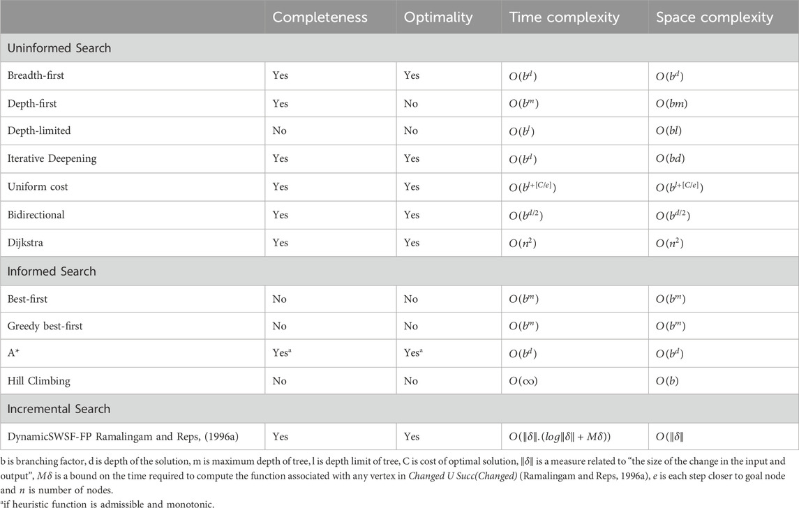
Table 1. Uninformed search, informed search (Russell and Norvig, 2003) and incremental search.
2.1.2 Informed (heuristic) search
The primary benefit of heuristic-based strategies is that the search space can be narrowed down. Many shortest path algorithms with a reduced search space have been proposed, such as best-first search (Pearl, 1984), greedy best-first search, hill climbing search, and A* (Hart et al., 1968) as shown in Table 1. These types of search methods attempt to narrow down the search space by utilizing various sources of additional information. Also, the A* algorithm is complete and optimal only if its heuristic function is admissible and monotonic, and many modern algorithms such as D* lite (Koenig and Likhachev, 2002) and LPA* (Koenig and Likhachev, 2001) are based on A*. Therefore, the A* algorithm stands out in the class of informed search because of its completeness and optimality.
2.1.3 Incremental search
Incremental search strategies are applicable for networks in which only a small number of link costs are likely to change at a time. Since these changes affect only a part of the graph, recomputing shortest paths for the entire graph is not necessary. Instead, it is possible to update paths corresponding to only a subset of the graph. As a result, such methods are used to solve dynamic shortest path problems, which require determining shortest paths repeatedly as the topology of a graph or its link costs only change partially. A representative incremental search algorithm is the Ramalingam and Reps’ algorithm (Ramalingam and Reps, 1996b) (RR), also known as the DynamicSWSF-FP algorithm. However, if all the link costs in the graph change, incremental search algorithms are unable to capitalize on previous search results.
2.1.3.1 DynamicSWSF-FP Algorithm
In dynamic transportation networks, often, only a portion of links change in terms of cost between updates. Starting costs for some of the nodes remain unchanged and thus do not need to be recalculated. As such, recomputing all the optimal routes could be wasteful since some of the previous search results can be reused. Incremental search methods, such as the RR algorithm, reuse information from previous searches to find the shortest paths for a series of similar path-planning problems, which is faster than solving each path-planning problem from the scratch. A key aspect about reusing previous search results is determining which costs have been affected by the cost update operation and must be recalculated. The RR algorithm employs two estimates: one that corresponds directly to starting distance in Dijkstra’s algorithm and another one is a right-hand-side value (rhs) for checking the local consistency to prevent path recalculation (Ramalingam and Reps, 1996b).
2.1.4 Reinforcement learning search
The field of RL has grown significantly over the past decades, with applications ranging from robotics (Polydoros and Nalpantidis, 2017), communications (Luong et al., 2019) to gaming AI (Vinyals et al., 2019). Among RL algorithms, Q-routing is a method that was proposed primarily for communication networks but can also be used in transportation systems (Boyan and Littman, 1994). Q-routing is based on Q-learning (Sutton and Barto, 2018) and does not need to know the link costs to start off, and can learn optimal paths over time through experience. In particular, for every node
where
In Equation 1,
As shown in Table 2, Q-routing requires less run-time complexity as it is executed more often. During training mode or offline mode, it takes

Table 2. Reinforcement Learning search.
3 Traffic network simulation
3.1 Traffic network description
A simple transportation network in the form of square grids is used in this study as shown in Figure 1A. The network has 25 nodes and 80 links (each 2-lane and directed).
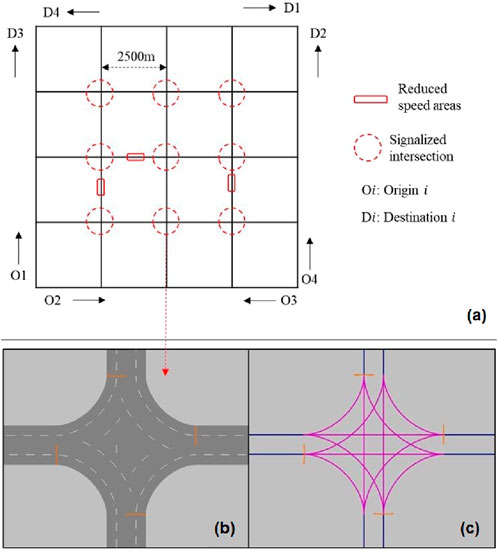
Figure 1. Details of the toy network used in the study. (A) Network shown in the form 5 x 5 square grids. (B, C): Signal heads and feasible movements at each intersection.
We have chosen to simulate a modestly sized network because of the following reasons. Dynamic rerouting of vehicles is highly influenced by accurate link travel cost estimations, which depend on interactions between vehicles. As such, microscopic traffic simulation is critical for capturing localized congestion effects. Smaller “toy networks” are commonly used for developing and validating methodologies [e.g. (Wang et al., 2022; Rampf et al., 2023; Bhavsar et al., 2014; Koh et al., 2020; Wang et al., 2022; Rampf et al., 2023; Bhavsar et al., 2014; Koh et al., 2020)]. Notably, variants of the Q-routing algorithm, such as the one developed in this study, are extensively utilized in large-scale communication networks [e.g. (Mammeri, 2019; Alam and Moh, 2022; Al-Rawi et al., 2015; Mammeri, 2019; Alam and Moh, 2022; Al-Rawi et al., 2015)] and have demonstrated robust performance. Given that transportation networks are typically much smaller and less complex than communication networks, at this time we will be validating the methods on smaller networks and explore larger scales in later studies.
In the 25-node network simulated in the current study, the length of each link is 2,500 m. To better capture heterogeneous flow conditions along these relatively long links, we split them into segments. Based on sensitivity analysis, we determined that a segment length of 25 m provides a reliable representation of link travel times. Further reducing the segment length does not significantly improve accuracy, and hence, links are divided into 100 equal-length segments. While our study uses equal-length segments for simplicity and consistency, we employed a general formula for computing weighted average speeds to account for potential scenarios where varying segment lengths might be necessary. For example, unequal segment lengths could be useful to represent varying geometries, such as curves or bottlenecks, along a link. However, in this study, such complexities were not required, and our approach ensures both computational efficiency and practical applicability.
The network is composed of nine signalized intersections. The signal heads and feasible movements at each intersection are shown in Figures 1B, C. Right turning movements are permitted on red. Through and left turning movements are simultaneously allowed (but controlled by the traffic signal). The node annotations and coordinates are shown in Figure 2. The four signal heads at an intersection are sequentially operated with a cycle length of 240 s (57s green + 3s amber per signal head). All the nine traffic signals are synchronized.
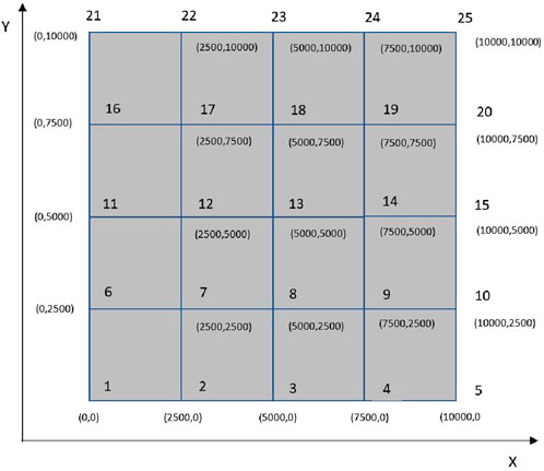
Figure 2. Node numbers and coordinates.
The demand for travel arises at two main origin intersections,
The aforementioned network is modeled in PTV VISSIM, which is a microscopic traffic simulator. As the size of a network increases, it becomes very tedious to determine and assign routes (sequence of links) for vehicles between several origin-destination pairs. Also, a predetermined route assignment in a simulation study does not reflect the route choices made by drivers in the real world (Fellendorf and Vortisch, 2020). Hence, the route choices are dynamically made in this study. The ability of VISSIM to compute dynamic stochastic user equilibrium is exploited to determine the routes dynamically. A comprehensive representation of route choice is thus possible. The vehicle composition of 90% cars and 10% heavy vehicles is used. Other parameters for the network simulation are as follows. The desired speed distribution used is shown in Figure 3. For the driving behavior model, the Wiedemann-74 car-following model is employed as it is considered suitable in urban environment. The default Car-following parameters used are:
• Average standstill distance: 2 m
• Additive part of safety distance: 2
• Multiplicative part of safety distance: three
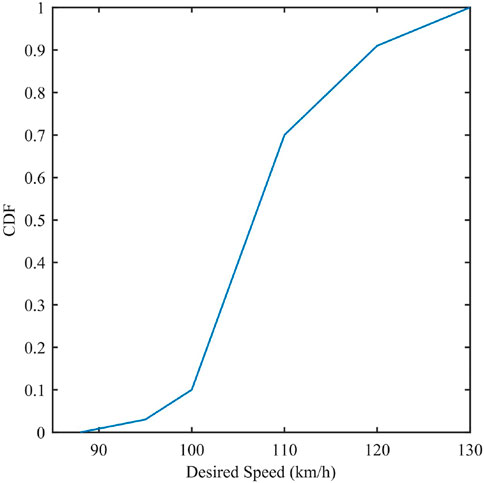
Figure 3. Speed distribution.
VISSIM also has a feature termed “reduced speed areas”, which is used to create temporary or localized congestion (e.g., a traffic incident). Three links are randomly chosen to introduce congestion as shown in Table 3. A simulation step size of 0.1s and a simulation period of 2 h are adopted. After every 100 simulation steps, the state of every vehicle in the network is sampled (and stored for further analysis) by using VISSIM COM. The state of a vehicle includes the link on which a vehicle is located, position on that link, lane occupancy, instantaneous speed, acceleration, and vehicle type.
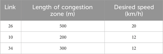
Table 3. Congested links.
The desired speed distribution within the congestion zone is as shown in Figure 4.

Figure 4. Speed distribution within the congestion zone.
3.2 Ground-truth link costs from simulation
To reliably measure ground-truth dynamic links costs we need to keep track of the spatial and temporal variation of link costs (travel times). The state of all the vehicles in the network is extracted from VISSIM after every 100 simulation steps. Every link between nodes i and j is considered to be composed of
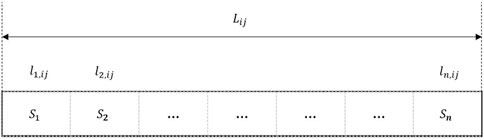
Figure 5. Segmentation of a link
The space mean speed of the segment
where,
4 Algorithm performance
4.1 Algorithm selection
From the related literature, it is clear that Dijkstra and
Figures 6–8 show the pseudocode for each algorithm. R1.5 The heuristic function that we use in the
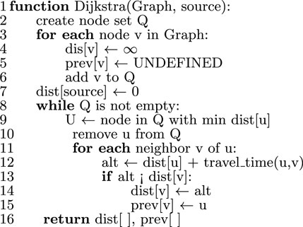
Figure 6. Dijkstra’s algorithm.
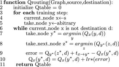
Figure 7. Q-routing algorithm.
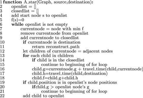
Figure 8. A* algorithm.
4.2 Algorithm performance
4.2.1 Static network
We first test the Dijkstra and A* algorithms on our simulated transportation network when there is no vehicle. The purpose of this test is to check the performance of the heuristic function in
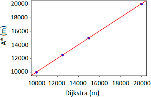
Figure 9. Q-Q plot between the optimal route costs for
4.2.2 Dynamic network
When traffic is introduced into the simulated network, the network becomes dynamic and link costs are estimated using methods described in Section 3.2. Dijkstra,
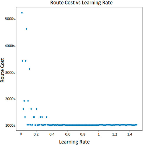
Figure 10. Route cost and learning rate for Q-routing.
In the dynamic simulated network,
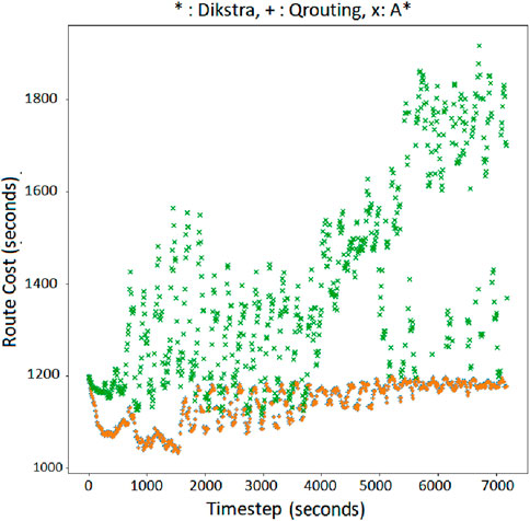
Figure 11. Minimum cost route for OD = (1,25) with Q-routing, Dijkstra (orange ‘+’), and
Based on Figures 11–14, it is clear that the
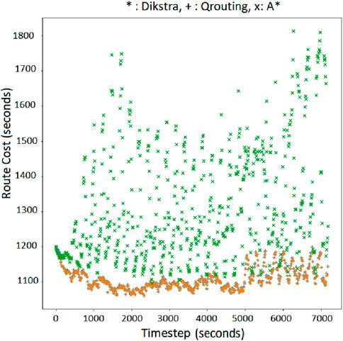
Figure 12. Minimum cost route for OD = 5,21 with Q-routing, Dijkstra (orange ‘+’), and A*(green‘x’).
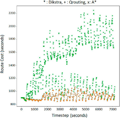
Figure 13. Minimum cost route for OD = 4,16 with Q-routing, Dijkstra (orange ‘+’), and A*(green ‘x’).
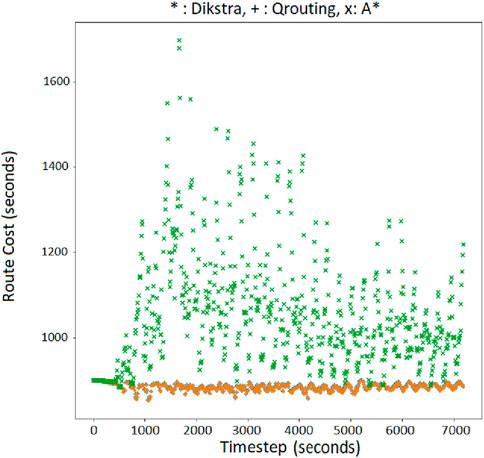
Figure 14. Minimum cost route for OD = 6,24 with Q-routing, Dijkstra (orange ‘+’), and A*(green ‘x’).
On the other hand, Q-routing delivers comparable route costs to Dijkstra during the entire simulation of the network. Following points should be considered while interpreting the plots in Supplementary Appendix Figures A1–A10 of Supplementary Appendix A. In a perfect information setting wherein the true link costs are accessible to the algorithm, it is well known that the Dijkstra algorithm gives the optimal shortest path between any two nodes of a network (Cormen et al., 2022). That is, Dijkstra gives the best-case cost when correct link costs are known. The costs corresponding to the Dijkstra algorithm shown in the plots of Supplementary Appendix Figures A1–A10 are those when Dijkstra was run as if the true costs were known. Although the true costs are not known in a realistic setting, the x-axis coordinates in the aforementioned Q-Q plots represent the theoretical upper bound of the performance for respective OD pairs. Along the y-axis we plot the costs produced by the Q-learning algorithm, wherein Q-learning is performing routing without knowing the costs. Thus, if in the Q-Q plot, the scatter is around the 45° line, it goes on to showing that the Q-learning algorithm, under an imperfect information setting, tends to perform close to an algorithm which gives the theoretical upper bound under perfect information setting. This is our main result, i.e., Q-learning tends to give near optimal result. Further, Supplementary Appendix B visualizes the agreement and differences in shortest routes estimated by Q-routing, Dijkstra and
5 Conclusion
In this paper, we have reviewed traditional shortest path finding algorithms, and have investigated RL-based search strategy, Q-routing, in a simulated transportation network. We have presented a comparison of Q-routing algorithms with the performance of two benchmark algorithms, namely, Dijkstra and A* in the network with dynamic link costs.
We have demonstrated the feasibility of Q-routing in a network with dynamically changing link-costs. We have shown that Q-routing estimates the cost route as minimal as Dijkstra’s and can be considered as an alternative optimal algorithm for finding the shortest path. Despite the time involved while learning the link-costs, during offline execution phase, Q-routing, however, may be executed with run-time complexity as equal as Dijkstra’s during online phase or subsequent runs. Also, Q-routing offers more options to expand the number of features used in estimating shortest path with a deep neural network to model an approximation of minimal travel time based on the number of selected features. On the other hand, with the dynamic link costs, the heuristic function of A* becomes less effective, producing suboptimal results. In a broader network scenario, a neural network can allow to learn statistics from from multiple network features such as the number of vehicles that enter the segment, segment length, number of lanes, current time of the day, and current weather conditions on the road. The cost function of the deep RL model might be a weighted combination of the output of the neural network and objective rewards (travel time, distance, operation cost, etc.), and the output of the model is still a policy to make the shortest path decision.
In this study, a number of factors may have limited the range of experimentation, i.e., whether it is possible to construct an A* guiding heuristic function based on estimated travel time, or it is challenging to simulate a city-scaled transportation networks for a more realistic case study. Also, not all algorithms reviewed in this paper are programmed since it is tedious to implement same-class algorithms that are computationally more expensive.
For future work, deep Q-learning (Van Hasselt et al., 2016) using a variety of architectures such as Graph Convolutional Networks (Zhang et al., 2019) and Graph Attention Networks (Veličković et al., 2018), can be integrated into the reinforcement learning based Q-routing to estimate shortest paths directly from network features such as traffic counts and link characteristics, rather than using a tabular-based estimation of minimal cost route and the link costs estimated from space-mean speeds as demonstrated in this paper.
Data availability statement
The raw data supporting the conclusions of this article will be made available by the authors, without undue reservation.
Author contributions
HP: Conceptualization, Data curation, Formal Analysis, Investigation, Methodology, Project administration, Resources, Software, Validation, Visualization, Writing–original draft, Writing–review and editing. SN: Resources, Software, Writing–original draft, Writing–review and editing. BM: Conceptualization, Funding acquisition, Methodology, Resources, Writing–review and editing. EM: Writing–review and editing. AA: Conceptualization, Formal Analysis, Funding acquisition, Investigation, Methodology, Resources, Visualization, Writing–review and editing.
Funding
The author(s) declare that financial support was received for the research, authorship, and/or publication of this article. The authors thank the UK Research and Innovation (UKRI) and the Natural Sciences and Engineering Research Council of Canada (NSERC) for funding this study (Grant Number: ALLRP 548594-2019).
Conflict of interest
The authors declare that the research was conducted in the absence of any commercial or financial relationships that could be construed as a potential conflict of interest.
Generative AI statement
The author(s) declare that no Generative AI was used in the creation of this manuscript.
Publisher’s note
All claims expressed in this article are solely those of the authors and do not necessarily represent those of their affiliated organizations, or those of the publisher, the editors and the reviewers. Any product that may be evaluated in this article, or claim that may be made by its manufacturer, is not guaranteed or endorsed by the publisher.
Supplementary material
The Supplementary Material for this article can be found online at: https://www.frontiersin.org/articles/10.3389/ffutr.2025.1524232/full#supplementary-material
Footnotes
1The use of the descriptor ‘Vehicular’ in VANETS should not be confused to imply as if they represent transportation or vehicular traffic networks. VANETS are mobile communication networks.
References
Alam, M. M., and Moh, S. (2022). Survey on Q-learning-based position-aware routing protocols in flying ad hoc networks. Electronics 11 (7), 1099. doi:10.3390/electronics11071099
Al-Rawi, H. A. A., Ng, M. A., and Yau, K.-L. A. (2015). Application of reinforcement learning to routing in distributed wireless networks: a review. Artif. Intell. Rev. 43(3), 381–416. doi:10.1007/s10462-012-9383-6
Bhavsar, P., Chowdhury, M., He, Y., and Rahman, M. (2014). A network wide simulation strategy of alternative fuel vehicles. Transp. Res. Part C Emerg. Technol. 40, 201–214. doi:10.1016/j.trc.2013.12.013
Boyan, J. A., and Littman, M. L. (1994). Packet routing in dynamically changing networks: a reinforcement learning approach. Adv. Neural Inf. Process. Syst., 671–678.
Chin, Y. K., Kow, W. Y., Khong, W. L., Tan, M. K., and Teo, K. T. K. (2012). “Q-learning traffic signal optimization within multiple intersections traffic network,” in 2012 sixth UKSim/AMSS European symposium on computer modeling and simulation (IEEE), 343–348.
Cormen, T. H., Leiserson, C. E., Rivest, R. L., and Stein, C. (2022). Introduction to algorithms. MIT press.
Dijkstra, E. (1959). A note on two problems in connexion with graphs. Numer. Math. 1 (1), 269–271. doi:10.1007/bf01386390
Ducrocq, R., and Farhi, N. (2023). Deep reinforcement q-learning for intelligent traffic signal control with partial detection. Int. J. intelligent Transp. Syst. Res. 21 (1), 192–206. doi:10.1007/s13177-023-00346-4
Farazi, N. P., Zou, B., Ahamed, T., and Barua, L. (2021). Deep reinforcement learning in transportation research: a review. Transp. Res. Interdiscip. Perspect. 11, 100425. doi:10.1016/j.trip.2021.100425
Fellendorf, M., and Vortisch, P. (2020). Microscopic traffic flow simulator vissim. Simul. Int. Ser. Operations Res. and Manag. Sci., 63–93. doi:10.1007/978-1-4419-6142-6_2
Fua, L., and Rilett, L. R. (2006). Heuristic shortest path algorithms for transportation applications: state of the art. Comput. Operations Res. 33, 3324–3343.
Hancock, P. A., Nourbakhsh, I., and Stewart, J. (2019). On the future of transportation in an era of automated and autonomous vehicles. Proc. Natl. Acad. Sci. 116 (16), 7684–7691. doi:10.1073/pnas.1805770115
Hart, P. E., Nilsson, N. J., and Raphael, B. (1968). “A formal basis for the heuristic determination of minimum cost paths,” in IEEE transactions on systems science and cybernetics (IEEE), 100–107.
Huang, Q.W., B., and Zhan, F. B. (2007). A shortest path algorithm with novel heuristics for dynamic transportation networks. Int. J. Geogr. Inf. Sci. 21 (6), 625–644. doi:10.1080/13658810601079759
Katre, P. R., and Thakare, A. (2017). “A survey on shortest path algorithm for road network in emergency services,” in International conference for convergence in Technology (I2CT).
Koenig, S., and Likhachev, M. (2002). “D* lite,” in Eighteenth national conference on artificial intelligence, 476–483.
Koh, S., Zhou, B., Fang, H., Yang, P., Yang, Z., Yang, Q., et al. (2020). Real-time deep reinforcement learning based vehicle navigation. Appl. Soft Comput. 96, 106694. doi:10.1016/j.asoc.2020.106694
Li, R., Li, F., Li, X., and Wang, Y. (2014). “Qgrid: Q-learning based routing protocol for vehicular ad hoc networks,” in 2014 IEEE 33rd international performance computing and communications conference (IPCCC), 1–8. doi:10.1109/PCCC.2014.7017079
Luong, N. C., Hoang, D. T., Gong, S., Niyato, D., Wang, P., Liang, Y.-C., et al. (2019). Applications of deep reinforcement learning in communications and networking: a survey. IEEE Commun. Surv. Tutorials 21 (4), 3133–3174. doi:10.1109/COMST.2019.2916583
Madkour, A., Aref, W. G., Rehman, F. U., Rahman, M. A., and Basalamah, S. (2017). A survey of shortest-path algorithms. arXiv preprint arXiv:1705.02044
Magzhan, K., and Jani, H. M. (2013). A review and evaluations of shortest path algorithms. Int. J. Sci. Technol. Res. 2 (6), 99–104.
Mammeri, Z. (2019). Reinforcement learning based routing in networks: review and classification of approaches. IEEE Access 7, 55916–55950. doi:10.1109/ACCESS.2019.2913776
Meerhof, J. (2021). Loop-breaking approaches for vehicle route planning with multi-agent q-routing. B.S. thesis. University of Twente.
Moreno-Malo, J., Posadas-Yagüe, J.-L., Cano, J. C., Calafate, C. T., Conejero, J. A., and Poza-Lujan, J.-L. (2024). Improving traffic light systems using deep q-networks. Expert Syst. Appl. 252, 124178. doi:10.1016/j.eswa.2024.124178
Pallottino, S., and Scutella, M. G. (1998). “Shortest path algorithms in transportation models: classical and innovative aspects,” in Equilibrium and advanced transportation modelling, 245–281.
Pearl, J. (1984). Heuristics: intelligent search strategies for computer problem solving, 48. Addison-Wesley
Polydoros, A., and Nalpantidis, L. (2017). Survey of model-based reinforcement learning: applications on robotics. J. Intelligent and Robotic Syst. 86, 153–173. doi:10.1007/s10846-017-0468-y
Ramalingam, G., and Reps, T. (1996a). On the computational complexity of dynamic graph problems. Theor. Comput. Sci. 158 (1), 233–277. doi:10.1016/0304-3975(95)00079-8
Ramalingam, G., and Reps, T. (1996b). An incremental algorithm for a generalization of the shortest-path problem. J. Algorithms 21 (2), 267–305. doi:10.1006/jagm.1996.0046
Rampf, F., Grigoropoulos, G., Malcolm, P., Keler, A., and Bogenberger, K. (2023). Modelling autonomous vehicle interactions with bicycles in traffic simulation. Front. Future Transp. 3, 894148. doi:10.3389/ffutr.2022.894148
Sunita Kumawat, C. D., and Kumar, P. (2021). “An extensive review of shortest path problem solving algorithms,” in Proceedings of the fifth international conference on intelligent computing and control systems.
Surekha, T., and Santosh, R. (2016). Review of shortest path algorithm. Int. Res. J. Eng. Technol. (IRJET) 3 (8), 1956–1959.
Sutton, R. S., and Barto, A. G. (2018). Reinforcement learning: an introduction. Cambridge, MA: MIT Press.
Swapno, S., Nobel, S., Meena, P., Meena, V., Azar, A. T., Haider, Z., et al. (2024). A reinforcement learning approach for reducing traffic congestion using deep q learning. Sci. Rep. 14, 30452. doi:10.1038/s41598-024-75638-0
Van Hasselt, H., Guez, A., and Silver, D. (2016). Deep reinforcement learning with double Q-learning. Proc. AAAI Conf. Artif. Intell. 30. doi:10.1609/aaai.v30i1.10295
Veličković, P., Cucurull, G., Casanova, A., Romero, A., Lio, P., and Bengio, Y. (2018). “Graph attention networks,” in International conference on learning representations.
Vinyals, B. I. C. W. M. e.a. O., Babuschkin, I., Czarnecki, W. M., Mathieu, M., Dudzik, A., Chung, J., et al. (2019). Grandmaster level in starcraft ii using multi-agent reinforcement learning. Nature 575, 350–354. doi:10.1038/s41586-019-1724-z
Wang, D., Gao, L., Lan, Z., Li, W., Ren, J., Zhang, J., et al. (2022). An intelligent self-driving truck system for highway transportation. Front. Neurorobotics 16, 843026. doi:10.3389/fnbot.2022.843026
Zhan, F. B. (1997). Three fastest shortest path algorithms on real road networks: data structures and procedures. J. Geogr. Inf. Decis. Analysis 1 (1), 70–82.
Zhan, F. B., and Noon, C. E. (1998). Shortest path algorithms: an evaluation using real road networks. Transp. Sci. 32 (1), 65–73. doi:10.1287/trsc.32.1.65
Keywords: shortest path, reinforcement learning, transportation network, dijkstra, A∗, dynamic link cost
Citation: Pham HD, Narasimhamurthy SM, Mehran B, Manley E and Ashraf A (2025) Reinforcement learning based estimation of shortest paths in dynamically changing transportation networks. Front. Future Transp. 6:1524232. doi: 10.3389/ffutr.2025.1524232
Received: 07 November 2024; Accepted: 10 February 2025;
Published: 06 March 2025.
Edited by:
Dongyao Jia, Xi’an Jiaotong-Liverpool University, ChinaReviewed by:
David López Flores, National Autonomous University of Mexico, MexicoWeizhen Han, Wuhan University of Technology, China
Copyright © 2025 Pham, Narasimhamurthy, Mehran, Manley and Ashraf. This is an open-access article distributed under the terms of the Creative Commons Attribution License (CC BY). The use, distribution or reproduction in other forums is permitted, provided the original author(s) and the copyright owner(s) are credited and that the original publication in this journal is cited, in accordance with accepted academic practice. No use, distribution or reproduction is permitted which does not comply with these terms.
*Correspondence: Ahmed Ashraf, YWhtZWQuYXNocmFmQHVtYW5pdG9iYS5jYQ==