Traffic capacity constraints from level 3 control transitions

With the increasing integration of conditionally automated Level 3 systems into real-world traffic, concerns about their impact on traffic efficiency and capacity have emerged. When such systems reach their operational limits, mandatory control transitions could disrupt traffic flow and reduce overall capacity. This study employs large-scale simulations and numerical experiments to analyze these effects and quantify potential capacity constraints. The results of the two-lane highway scenario show an experimental capacity reduction of up to $2000\text{veh/h}$ in an almost fully automated but unmanaged traffic mix, corresponding to a loss of about $60\%$. Control transition-related effects become increasingly pronounced at a Level 3 penetration rate between $10\%$ and $20\%$. Estimated capacity reductions suggest that the maxima in time headway increments during the transition phase contribute most to these effects.

1 Introduction

As manufacturers begin to introduce Level 3 automated driving systems to the market, the potential impact of such systems on overall traffic flow and capacity needs to be investigated. A key challenge arises from the fact that Level 3 systems require human drivers to take over control when reaching system limits, leading to so-called transitions of control (ToC), which may disrupt traffic flow and reduce road capacity. Despite regulatory advancements concerning Level 3 systems (R157 by UNECE (2023)), the macroscopic impact of such procedural ToC effects on traffic conditions remains insufficiently explored. This raises the general question of how Level 3 control transitions in conditionally automated vehicles (AVs) affect traffic capacity and, more specifically, what characteristics of procedural ToC-induced time headway increments in vehicle strings contribute to this effect. To investigate this, we conduct a large-scale simulation-based analysis and complement it with simplified numerical experiments to estimate macroscopic capacity impacts. Our study also explores the underlying mechanisms of the transition phase in greater detail. Existing research on potential capacity gains from AVs, as exemplified by Friedrich (2016) and Park et al. (2021), has primarily focused on higher automation levels (4–5) under optimistic assumptions of short time headways, e.g., ${\tau }_{AV}=0.5$ s, in contrast to observed headways in manually driven vehicles of at least $1\text{s}$ in freeway traffic, depending on vehicle speed, as shown by Wagner (2012). Our previous work in Alms et al. (2022) and Alms and Wagner (2024) touched on ToC-related capacity effects but lacked a comprehensive quantification of resulting capacity losses. This study addresses these gaps by (i) adopting a macroscopic perspective using realistic, R157-compliant time headways of ${\tau }_{AV}=1.6$ s, and (ii) introducing an exploratory estimation approach that explicitly accounts for Level 3 disengagements in road capacity assessment.

The rest of the paper is organized as follows: Section 2 introduces the conceptual aspects of ToCs in Level 3 automated systems. In Section 3, we present a highway scenario calibration based on real-world detector data. Section 4 details our methodology for investigating ToC-related capacity effects in a simulation study, while Section 5 presents and discusses our results, comparing simulated and estimated capacity reductions. Lastly, Section 6 offers our perspective on the interpretation and limitations of this study.

2 Transitions of control in level 3 automated driving

The six levels of driving automation, defined by SAE International (2021), not only classify automated driving functions and capabilities but also specify the human driver’s role in terms of engagement and responsibility, as illustrated in Figure 1. Conditional automated driving (Level 3, highlighted with a purple frame in Figure 1) represents a fundamental shift toward automated vehicle operation within defined Operational Design Domains (ODD), specified in British Standards Institution (2020), allowing human drivers to disengage from the primary driving task. However, if the Level 3 system requires the driver to resume control, a takeover request (ToR) is issued, initiating a critical transfer of authority: these procedures are referred to as transitions of control (ToC, plural: ToCs). Detailed insights into various aspects of ToCs are available through a comprehensive literature review on takeovers in automated driving (McDonald et al., 2019). Further studies examine the intricacies of modeling human factors, such as situational awareness and task demand (Van Lint and Calvert, 2018; Calvert and van Arem, 2020), or reduced driver performance (Wang et al., 2025b), during ToCs.

Figure 1

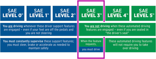
Figure 1. Excerpt from Shuttleworth (2019)’s illustration of the SAE Levels of Driving Automation (SAE International, 2021), with Level 3 highlighted by a purple frame.

The current regulations R157 from UNECE (2023) specify technical requirements for the certification of Level 3 Automated Lane Keeping Systems (ALKS) and set the time range $T_{\text{lead}}$ to $10\text{s}$ before a failed transition escalates to a minimum risk maneuver (MRM), which is critical for the process of control transitions. Within the context of the EC project (TransAID, 2021; Lücken et al., 2019; Mintsis et al., 2019) introduced a novel ToC model, which is fully parametrizable to align with these later-established UNECE specifications and for which a detailed description of the model’s implementation is provided. The operationalization of ToCs is further specified in the ongoing EC project Hi-Drive (Bolovinou et al., 2023; Sauvaget et al., 2023) and demonstrated in Schulte-Tigges et al. (2023).

Figure 2 illustrates the basic mechanisms of the ToC model for successful and failed control transitions implemented in the microscopic traffic simulation SUMO (Alvarez Lopez et al., 2018). After a ToR, the AV enters a preparatory phase characterized by headway enlargement and disabled lane changing. Automated driving continues for the limited lead time, after which either the driver resumes control in time (successful transition), or, if not, the AV initiates an MRM (failed transition). For failed transitions, the AV initiates a phase of constant deceleration and may come to a full stop if the human driver does not respond. Although such events are rare, they can have a high impact and are the subject of extensive safety investigations based on disengagement reports (e.g., (Ward, 2024; Kohanpour et al., 2025)). However, this aspect is not the focus of the present work. In the case of a successful transition, the driver state model accounts for a phase of reduced human driving performance, with recent studies gaining further insights into both post-ToC durations (Wang et al., 2025a) and potential negative impacts on traffic stability (Wang et al., 2024).

Figure 2

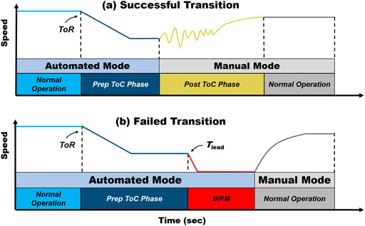
Figure 2. ToC model operation modes illustrated in a representative speed-time diagram for: (a) successful transition and (b) failed transition.

In Maerivoet et al. (2019) and Lücken et al. (2019) principal transition phase effects of consecutive, quasi-synchronous ToCs in a platoon of Level 3 automated vehicles were previously demonstrated. Figure 3a, which depicts speed and time headways for a string of five AVs disengaging at the same location, illustrates this effect in a simplified simulation experiment with identical vehicle parametrization. The increased time headways, and consequently the cumulative speed reduction, are caused by the preparatory headway increment of the vehicle automation to facilitate a safe takeover (cf. Figure 2, Prep ToC Phase). Figure 3b extends this analysis by showing acceleration profiles for a larger platoon of up to 32 vehicles—the maximum size at which the last AV still manages to prevent a complete stop—using SUMO’s ACC model for AVs, based on Xiao et al. (2017). The main observed effects in the vehicle decelerations include:

$•$ With a moderate default deceleration of $1{\text{m/s}}^2$ during the $10\text{s}$ transition phase specified by R157, maintaining safe gaps in AV platoons is not feasible without initiating deceleration earlier. Panel (b-2) in Figure 3b illustrates that, starting with the first vehicle behind AV.1 (dark blue line), SUMO’s gap controller begins to decelerate even before the respective vehicles receive ToRs to initiate their ToC.

$•$ Starting with AV.20, the following vehicles must decelerate more aggressively than their target deceleration of $1{\text{m/s}}^2$. Panel (b-3) in Figure 3b highlights these deceleration overshoots for AV.24–28. These overshoots are specific to the ACC model, while similar experiments employing SUMO’s default model do not exhibit this behavior. However, that model compensates by initiating deceleration even earlier than the ACC model. The principal accumulation effect of consecutive ToCs remains present in both cases.

Figure 3

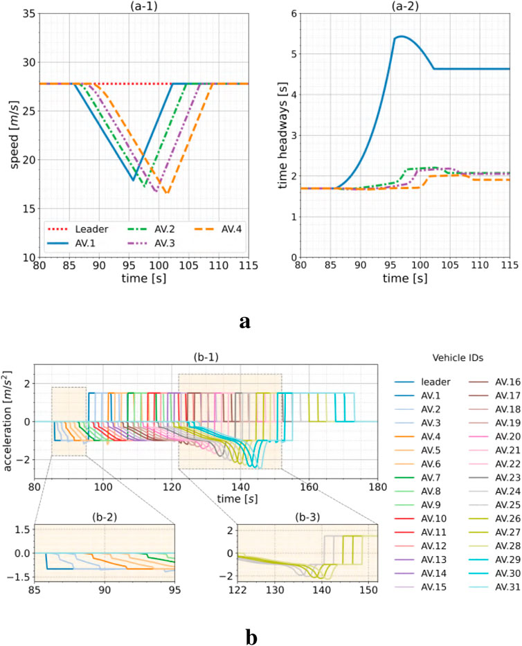
Figure 3. Platoon simulations with consecutive ToCs performed at a fixed location. (a) shows speed and time headway profiles for a short platoon with five AVs, illustrating the headway increment effect. (b) depicts acceleration profiles for a platoon of 32 AVs, showing an escalating headway increment effect with SUMO’s ACC model.

These numerical experiments are highly simplified due to identical vehicle parametrizations, yet they effectively illustrate the isolated ToC effects discussed. Given the cumulative deceleration patterns observed, we expect that ToC-induced disturbances may lead to noticeable reductions in traffic capacity. To examine whether these effects also manifest under more realistic traffic flow conditions, we calibrate a SUMO simulation scenario to detector data in Section 3.

3 Calibrating SUMO for a highway traffic scenario

To analyze the impact of ToCs on traffic capacity, we use real-world detector data from a German highway west of Berlin as a reference for SUMO calibration. The following sections detail the dataset and simulation setup.

3.1 AVUS detector data

Figure 4a shows a section of the Bundesautobahn A115, referred to as AVUS, which was occasionally used as a motor racing track in the past and is a highly frequented highway with up to 80.000 vehicles per day. We hypothesize a potential ODD zone for Level 3 automated driving in the inbound segment of the road (cf. Figure 4a, panel (a)), which is a two-lane highway with speed limits of $80\text{km/h}$ starting at an interchange section and increasing to $100\text{km/h}$ up to the next traffic exit, that is located nearly $5\text{km}$ downstream. The inbound traffic data on the two-lane section come from a detector at an underpass (cf. Figure 4a, panel (c)). After this point, the road has a slight slope for a few hundred meters, but the exact gradient could not be verified. A ramp merges onto the main edge about $600\text{m}$ downstream, from where the speed limit increases to $100\text{km/h}$.

Figure 4

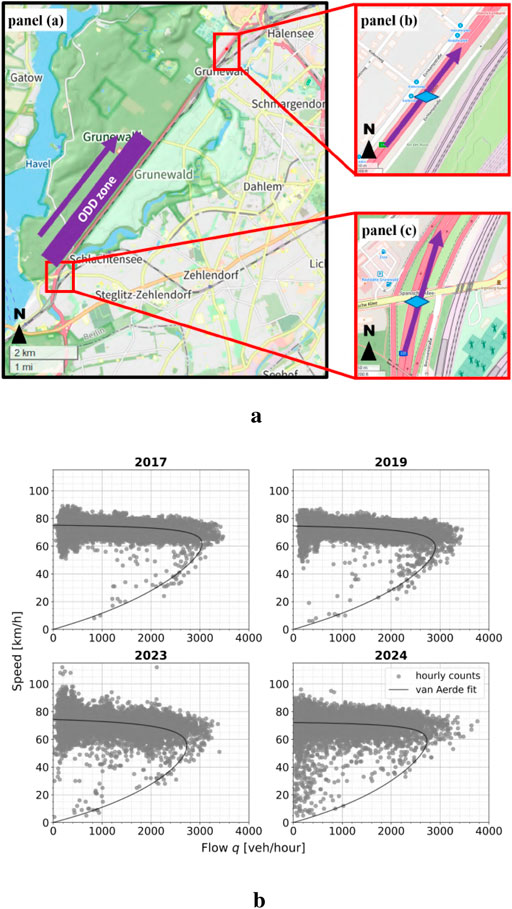
Figure 4. Overview of the AVUS scenario. (a) OpenStreetMap view of the AVUS highway with a potential 5 km ODD zone on the two-lane inbound edge highlighted in purple. Zoom displays show traffic detector locations, marked with blue in subpanels (b) and (c). Purple arrows indicate the inbound traffic direction. (b) Speed–flow scatterplots of yearly AVUS detector data for inbound traffic from detector “TE002”.

Figure 4b displays speed—flow relations for several years of the AVUS between 2015 and 2022, as scatterplots based on data from Digitale Plattform Stadtverkehr Berlin (2024). These data are originally tagged as hourly flows with corresponding average speeds per hour, but we suspect that this is not accurate. While the number of vehicles is accumulated over a full hour, the high variations in speeds at lower flow rates suggest that these data points from the detector database might actually represent speed averages over intervals of 1 minute or less. We were unable to verify this suspicion directly with the publisher of the data, but we argue that the actual speed value recorded in the database is likely the last entry of a full hour — possibly for efficiency and memory-saving reasons in data processing — rather than the average speed over the entire hour. This ultimately results in a notably wider distribution of speed values at lower flow rates than expected for true hourly data. For reference, we also added the model fit developed by Van Aerde (1995) to each plot.

Table 1 lists the yearly maximum flows $q$, the $95^{\text{th}}$ and $99^{\text{th}}$ percentiles as suggested by Brilon and Geistefeldt (2010), and the deterministic capacity derived from the van Aerde model, as well as the corresponding shares for heavy good vehicles (HGVs) extracted from the raw detector data between 2016 and 2024. Additionally, data provided by the BASt (2025) from a detector downstream of the AVUS at “Eichkamp” are also included in the table for comparison (cf. Figure 4a, panel (b)). Note that 2024 shows an oddly high HGV share, which we consider very unlikely and attribute to recent technical changes in sensor-based detection and data processing by the provider. The report from BASt (2021) stated a nationwide HGV share of $18.1\%$ in 2021 on Germany’s highways.

Table 1

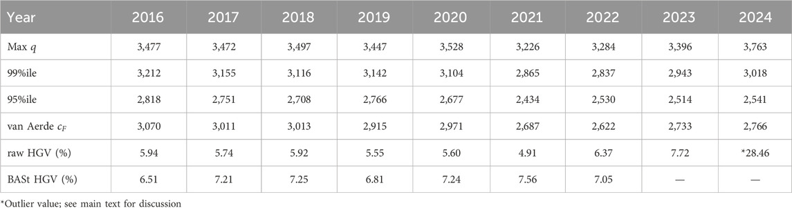
Table 1. Yearly flow metrics and HGV shares for AVUS inbound traffic.

3.2 Simulation setup for calibration

To investigate the impacts of ToCs in mixed-autonomy traffic, we compose a traffic mix of four different vehicle types: automated passenger vehicles (AVs), manual passenger vehicles (MVs), light goods vehicles (LGVs), and heavy goods vehicles (HGVs). The most relevant parameters for a heterogeneous traffic behavior in this AVUS highway scenario are visualized in Figure 5. Instead of utilizing SUMO’s default parameters, vehicle type specific distributions were deployed. Table 2 presents the full parametrization scheme for all vehicle types.

Figure 5

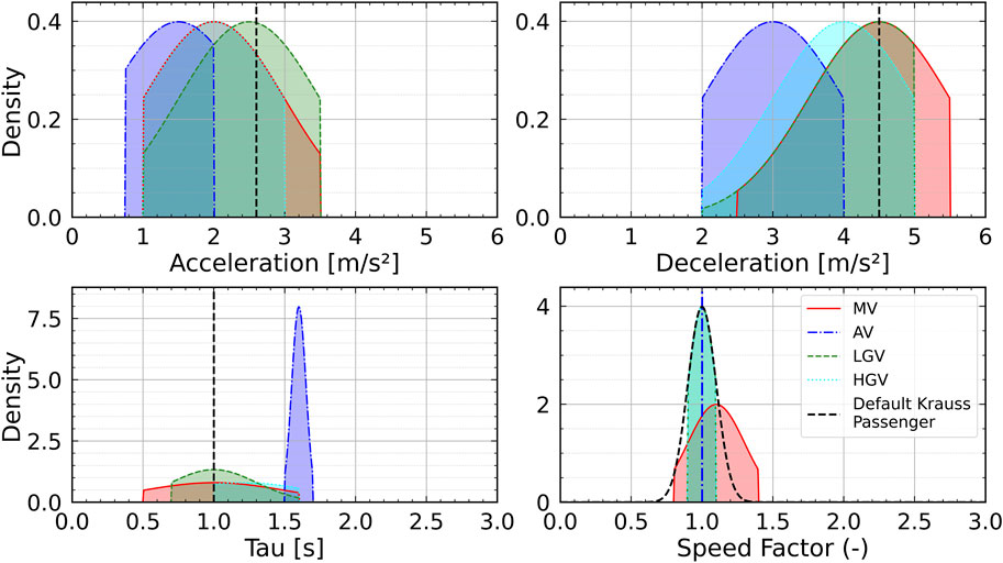
Figure 5. Distributions of the main parameters for different vehicle types. SUMO’s default is indicated by the black dashed line.

Table 2

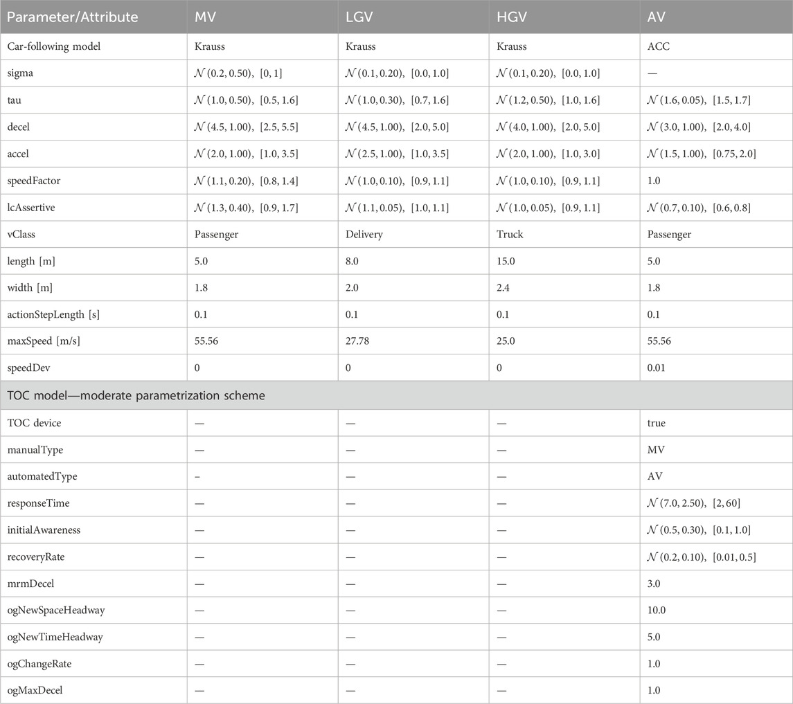
Table 2. Vehicle type definitions. “—” indicates not defined.

In principle, SUMO’s vehicle insertion capacity exceeds that of comparable real-world traffic scenarios. Therefore, we aim to calibrate the simulation primarily to match the maximum flow $q$ in relation to the real-word AVUS data. Besides the general vehicle parametrization, two insertion properties in SUMO heavily effect the overall capacity of a simulation, i.e., the vehicle speed at insertion departSpeed and lane choice at insertion departLane. We kept these parameters unchanged for all simulations in the paper. The most important capacity related SUMO options are defined as follows:

$•$ departSpeed = max

$•$ departLane = random (AV,MV,LGV)

$•$ departLane = right (HGV)

$•$ extrapolate-departpos = true

$•$ step-length = 0.1 s

3.3 Calibration including ramp flow

In the first step, we ran simulations with increasing demand using MVs only. To better capture the full spectrum of the fundamental diagram in SUMO, we introduced additional vehicle flow on the incoming ramp. This creates a merging scenario, leading to traffic breakdown upstream of the main edge’s detector position. Figure 6 shows the speed–flow relations as scatterplots for (i) real-world detector data from 2024, (ii) SUMO’s default parametrization, and (iii) the aggregated main edge data from the final calibration. The graphic also color-codes the demand intensities from the on-ramp and highlights the maximum $q$ of the AVUS detector data 2024. For reference of the expected average speeds defined by the german Highway Capacity Manual—referred to as HBS—in (FGSV, 2015, Part A, Figure A3-10) for a two-lane highway (slope $\le 2$, speed limit $80\text{km/h}$), a black solid line was added.

Figure 6

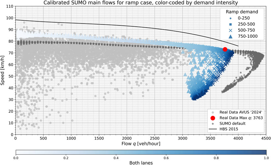
Figure 6. Speed–flow relations for the AVUS scenario, including ramp flow, comparing calibrated flows based on the parametrization scheme from Table 2 versus AVUS detector data from 2024, and SUMO’s default. The main edge’s demand intensities are color-coded in blue. Ramp demand levels are coded by marker size and style.

The key findings derived from Figure 6 are:

1. Comparing the dark gray SUMO default data with the light gray detector data, we identify how far SUMO’s default exceeds the actual maximum flow (about 700 vehicles surplus).

2. The calibrated main edge’s flow (blue-colored points) is notably lower than SUMO’s default. Maximum flows (dark blue points) are much closer to the real-data (about 130 vehicles difference) compared to SUMO’s default (dark gray).

3. The overall speed–flow relation of the calibrated main edge (blue) is slightly tilted toward higher speeds compared to SUMO’s default (dark gray), and the speed gradient more in line of the HBS expectation (black line).

4. The calibrated main edge’s traffic breakdown on the congested side of the fundamental diagram (indicated by darker-colored blue points) is much less pronounced than what is to be expected from real-world data (see light gray scatter points).

The phenomenon described in point 4 is, in part, a limitation of SUMO’s current modeling of cooperative lane-changing behavior between neighboring lanes under traffic breakdown conditions. Correspondingly, Figure 7 compares the lane-specific calibrated flows in SUMO with real AVUS data from 2024. We clearly identify the disparate speed levels between the lanes in SUMO (bottom panel), whereas the real-world data (top panel) indicate similar speed–flow relations on both lanes. Rummel (2017) indirectly revealed this issue in his investigation but was unable to unequivocally identify the lane-specific breakdowns as the underlying cause of SUMO’s oversaturation compared to the HBS predictions, nor did the report by Geistefeldt et al. (2017), which ultimately disregarded SUMO in its analysis for this very reason. While this limitation prevents a full replication of the real-world dynamics, we proceed with the calibration of the scenario as a basis for our analysis and will address this shortcoming in our future work.

Figure 7

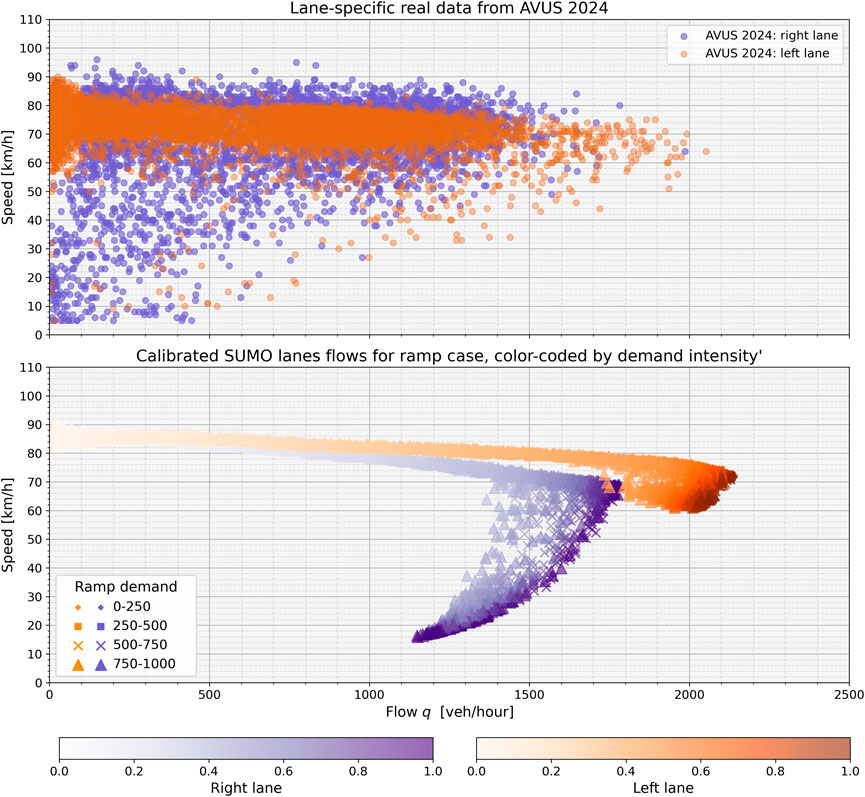
Figure 7. Lane-specific speed–flow relations for real data from 2024 (top panel) and SUMO’s calibrated ramp scenario (bottom panel).

3.4 Refining calibration by incorporating HGV share

In a second step, based on the parametrization scheme plausibilised for MVs in the ramp scenario (cf. Table 2), we conducted simulations with different shares of HGVs, LGVs, and MVs, but without any ramp flow. As a result, we can no longer reproduce the entire fundamental diagram for this highway scenario, since SUMO’s flow does not naturally lead to a traffic breakdown as observed in real-world highway traffic. The reason we need to disregard the unstable part of the fundamental diagram at this point is technical: SUMO does not maintain precise LGV/HGV shares for vehicle insertions when approaching maximum flow. Instead, the share of LGVs and HGVs declines to zero until SUMO can only insert MVs when the traffic breakdown at capacity is expected. This behavior stems partly from the parametrization of LGVs and HGVs, such as their larger vehicle lengths and time headways.

Figure 8 shows the speed–flow relations for the main edge with LGV/HGV shares of $0\%,5\%,10\%$, and $15\%$ (LGV/HGV distributed as $2/3$ vs. $1/3$), compared to AVUS detector data from 2018. The key findings are as follows:

1. The maximum flow with a $0\%$ HGV share (purple-colored scatter points) is almost the same as in the ramp case (cf. Figure 6, purple markers), with a difference of about $50\text{veh/h}$.

2. The AVUS detector data from 2018 have an HGV share of $6\%$, with a maximum flow of $3497\text{veh/h}$. The speed variation in the detector data, particularly for lower demands, is very high, which we attribute to factors discussed in Section 3.1.

3. The speed variations in all simulation results are relatively large. This is expected, as we deliberately plotted only the average speeds of the last 1-min interval of a full hour, which we suspect is also the case for the real detector data. This illustrates a plausible speed distribution from the calibrated simulations compared to the detector data.

4. The color-coded flows at capacity decrease notably with increasing HGV shares (decline by 260 to $410\text{veh/h}$).

Figure 8

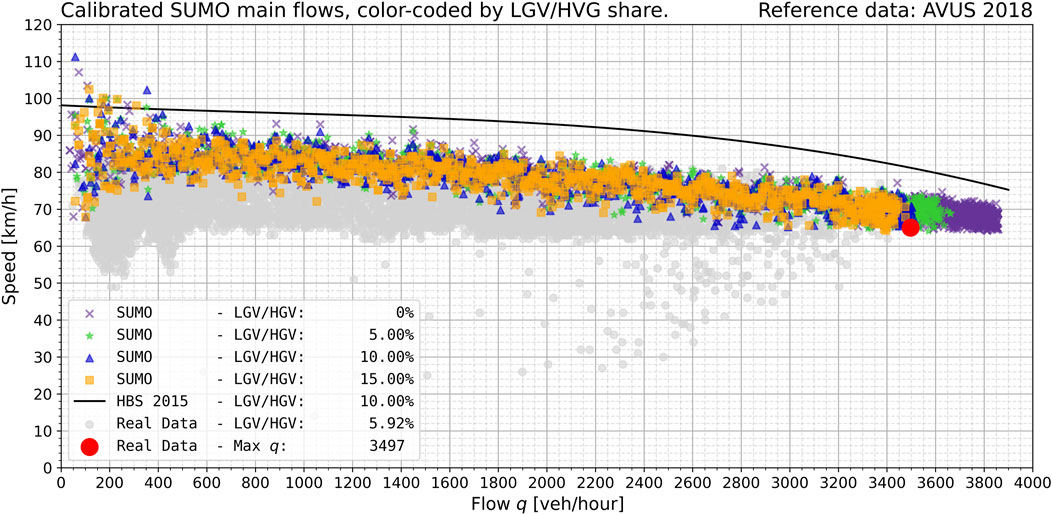
Figure 8. Speed–flow relations for the AVUS scenario based on the parametrization scheme from Table 2 comparing calibrated main flows considering LGV/HGV shares. Real-world detector data from AVUS 2018; color-coding by LGV/HGV share.

Considering the relatively low deterministic capacities based on the AVUS detector data stated in Table 1 compared to the expected capacities from the HBS (range from 3,600 to $3900\text{veh/h}$) for this highway type, we assess our SUMO calibration in terms of capacity as follows:

$•$ The maximum flow in the SUMO ramp scenario without HGV share consideration is $3907\text{veh/h}$. The 95th and 99th percentile flows are $3853\text{veh/h}$ and $3882\text{veh/h}$, respectively. The van Aerde model estimates a maximum flow of $3665\text{veh/h}$ based on SUMO data. These values are significantly higher than the detector data but do not account for HGV shares in SUMO.

$•$ With HGV share consideration the maximum flows on the stable arm of the fundamental diagram decrease notably between 6.7 to $10.5\%$ as illustrated in Figure 8.

Under the assumption that those percentages under HGV consideration scale down proportionally in SUMO with the capacity numbers stated above, we obtain the following deterministic capacity ranges for the calibrated parametrization scheme:

$•$ Max flow: $3497-3647$ veh/h

$•$ 95th percentile: $3449-3597$ veh/h

$•$ 99th percentile: $3475-3624$ veh/h

$•$ van Aerde model: $3281-3421$ veh/h

Even though these capacities are still about $200-300\text{veh/h}$ larger than the detector numbers in Table 1, we consider this an adequate calibration, particularly compared to SUMO’s default, since the real-world detector flow data are overall lower compared to the HBS range, which we identified to be between 3,600 and $3900\text{veh/h}$. Other local factors, such as road curvature, slope, shoulder lane width, underpass length, or surface conditions, which might impact the local capacity and could explain the rather low detector-based flows, are unknown to us. While more detailed microscopic calibration using high-resolution trajectory data (e.g., as in Schrader (2024) or Liu et al. (2024)) would be desirable, such data were not available for this study.

4 Methodology to quantify capacity effects of ToCs

To determine ToC-related capacity impacts, we conduct a simulation study with an increasing AV penetration rate and measure the corresponding maximum flows $q$. Additionally, we estimate the anticipated ToC-induced capacity reduction and later compare these estimates with the measured results from the simulation study.

4.1 Simulation experiment

Algorithm 1

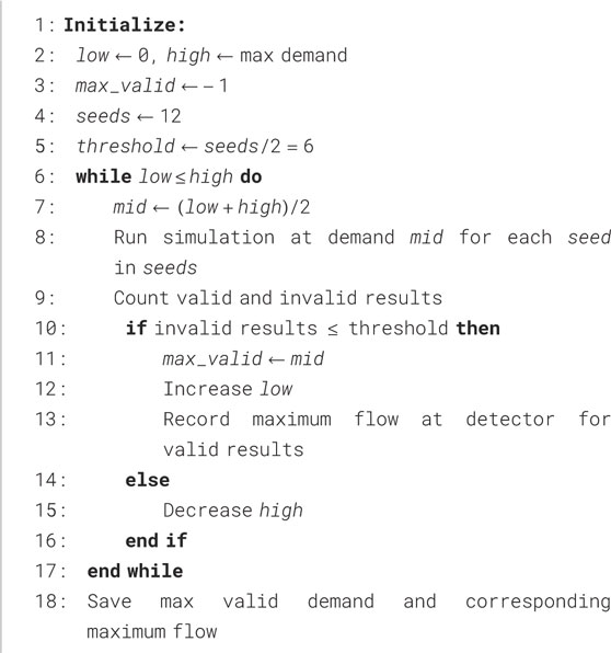
Algorithm 1.Binary search for maximum flow.

For the simulation study, we define a wide range of traffic shares based on the vehicle types outlined in Table 2. The traffic compositions feature increasing AV shares (AV00–AV85) in $10\%$ increments, with AV increases and MV decreases of equal size, and a constant LGV/HGV share of $15\%$ (split $2/3$ LGV, $1/3$ HGV). Considering a hypothetical ODD zone on the AVUS inbound highway, as illustrated in Figure 4a, AVs are assumed to be capable of Level 3 automated driving at speeds of up to $100\text{km/h}$ until reaching the end of the ODD zone. Vehicles enter the network in their respective driving mode at random on one of the two lanes, except for HGVs, which are only inserted on the right lane. They continue their trip until reaching the end of the AVUS, near the detector position highlighted in Figure 4a, panel (b). Four distinct scenarios are examined, differing in how ToCs are facilitated:

1. No ToCs: Simulations without any ToCs.

2. Unmanaged: Simulations with unmanaged ToCs at the end of the ODD zone.

3. Managed: Simulations with ToCs managed by a ToC-dispatch algorithm over the full length of the ODD zone.

4. Unmanaged “rightmost95”: Simulations with unmanaged ToCs at the end of the ODD zone, emulating the concept of the latest approved manufacturer system by Mercedes-Benz Group (2024), operating up to $95\text{km/h}$ on the rightmost lane, without overtaking.

For cases 2–4, we additionally run simulations with $\tau$-distributions for MVs around ${\tau }_{MV}=0.8\text{s}$ and $1.2\text{s}$. In case 3, we deploy the heuristic algorithm developed by Lücken et al. (2019). The control algorithm basically emulates a V2X-based traffic management scheme by dispatching ToRs to AVs in a coordinated manner to mitigate the accumulation effect of consecutive ToCs. For case 4, AVs are only inserted into the simulation on the rightmost lane, overtaking is disabled, and their speed is limited to $95\text{km/h}$.

To measure the capacity per AV share as precisely as possible, we run the AVUS scenario with 12 seeds per traffic mix, deploying a binary search as illustrated in Algorithm 1. To ensure we obtain the correct maximum flow, the results of each run must be checked against the actual traffic share versus the expected share due to SUMO’s insertion mechanism, as described in Section 3.4. The binary search continues increasing the demand as long as valid traffic shares are observed, until the maximum flow per simulation run is reached.

Simulations run with a $30\text{min}$ warm-up phase to populate the scenario and then record data for a full hour of simulated time (SUMO version 1.22 from Alvarez Lopez et al. (2025)). A detector near the end of the ODD zone records speed and flow to identify potential traffic breakdowns and measures the maximum flow. Figure 9 exemplarily shows spatiotemporal heatmaps of the ODD zone for speed and flow. Figures 9A,B, result from the same demand level and AV share—only the seed values, which determine the randomization process of vehicle insertions, differ.

Figure 9

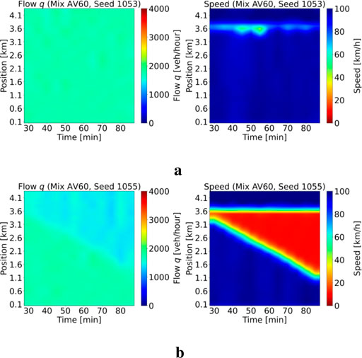
Figure 9. Spatiotemporal heatmaps of the ODD zone for speed and flow. (a) Valid run at max capacity: Mix AV60, seed 1053. (b) Invalid run: Mix AV60, seed 1055. The traffic breakdown is clearly visible in speed and flow.

4.2 Estimating capacity reduction

Considering the minGap in SUMO as $g_{\text{min}}$, individual vehicle lengths $l_i$, type-specific ${\tau }_i$, and varying vehicle shares $p_i$, the theoretical lane capacity $C$ at speed $v$ is given by:

$C=\frac{v}{{\sum }_i{p}_i\cdot \left(l_i+g_{\text{min}}\right)+v{\sum }_i{p}_i\cdot {\tau }_i}(1)$

For the SUMO default minGap of $2.5m$, a speed $v=100km/h$, and the respective vehicle lengths and $\tau$-values from Table 2, we compute lane capacities across all traffic mixes. Assuming a constant time headway ${\tau }_i$ for each vehicle type, without considering ToCs, the resulting capacities per mix are shown in Figure 10a. The results demonstrate that as the $\tau$-values for MVs increase (${\tau }_{\text{MV}}=0.8\text{s}$ to ${\tau }_{\text{MV}}=1.2\text{s}$), while keeping fixed values for AVs $({\tau }_{\text{AV}}=1.6\text{s})$, LGVs $({\tau }_{\text{LGV}}=1.0\text{s})$, and HGVs $({\tau }_{\text{HGV}}=1.2\text{s})$, the decline in maximum capacity across traffic mixes becomes less pronounced. If MVs had the same $\tau$-value as AVs—in this case, ${\tau }_{\text{AV}}=1.6\text{s}$ — the lane capacities would remain stable, regardless of the increasing AV share.

Figure 10

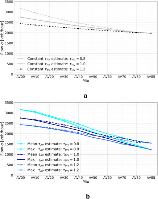
Figure 10. Estimated lane capacities based on Equation 1 for varied mean τ_MV-values. (a) shows capacity estimates assuming a constant τ_AV (no ToC consideration). (b) accounts for increasing τ_AV due to ToC effects (with ToC consideration).

To account for ToC effects in such estimations, we repeat the simplified numerical experiment with the 32-vehicle platoon described in Section 2, this time varying the AV–MV share in 10%-intervals between the two vehicle types. The top panel in Figure 11a shows the time headway profiles for a 100% AV share, corresponding to the acceleration profile discussed in Figure 3b. The increasing headways for later-following AVs are clearly identifiable. In the bottom panel (Figure 11b), which depicts a 50–50 share, the headway increase is far less pronounced compared to the top panel.

Figure 11

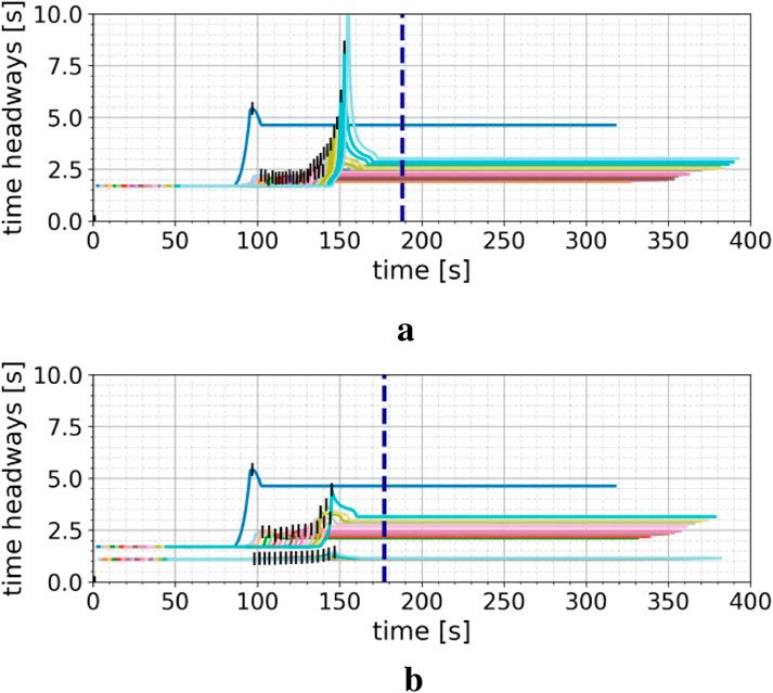
Figure 11. Time headways in a platoon experiment with 32 vehicles and varying AV–MV shares. Black markers indicate the maximum headway for each vehicle. The vertical blue dashed line marks the onset of system-wide headway stabilization (see text for criterion), after all ToCs are completed. (a) 100% AV vs. 0% MV share. (b) 50% AV vs. 50% MV share.

Therefore, we introduce two additional estimators. In Equation 1, instead of using a fixed ${\tau }_{AV}=1.6\text{s}$, we derive ${\tau }_i$ for each share $p_i$ from the numerical experiments as follows:

$•$ Max: The black markers in Figure 11 denote the maximum time headway of each vehicle in the simulation run. The average of these maximum values serves as ${\tau }_i$ for each $p_i$ in the estimator max.

$•$ Mean: The point at which headways have stabilized after all ToCs are completed is marked by the vertical blue dashed line in Figure 11. Stabilization in this experiment is defined as the latest point after all headway peaks at which all vehicles’ headways remain constant to within $\pm$0.005 s for at least 15 s. The average of the time headways at this point serves as ${\tau }_i$ for each $p_i$ in the estimator mean.

With these estimator-based $\tau$-values, the original capacity Equation 1 is adjusted by replacing the fixed headway term in the denominator with $v{\sum }_i{p}_i\cdot {\widehat{\tau }}_i(p_i)$, where ${\widehat{\tau }}_i(p_i)$ is the empirically derived time headway for AVs as a function of their share $p_i$, while other vehicle types retain fixed values. The estimators max and mean provide these AV-specific headways based on the numerical experiments. Figure 10b presents the results of the calculations that account for ToCs by utilizing these estimators. Both trends exhibit a notable decline in estimated lane capacity compared to the ToC-ignorant estimation depicted in Figure 10a.

5 Results and discussion

Figure 12 presents the overall results obtained from the simulation study outlined in Section 4.1. First, we find that all maximum flows in the AV00 share, ranging between $3405-3611\text{veh/h}$, fall within the expected capacity range from the calibration, i.e., $3281-3647\text{veh/h}$. We further analyze these results in detail for the four scenarios, following the order in which they were previously defined:

1. No ToCs: The results (green line) show that up to share AV40, maximum flows remain relatively stable, with a reduction of approximately $100\text{veh/h}$ compared to AV00. Beyond AV50, flow values begin to increase again. This trend can be linked to a homogenization effect in traffic flow as AV shares grow, which is influenced by the AV parametrization—-specifically, the absence of sigma and a very small speedDev value of 0.01.

2. Unmanaged: In the case of entirely unmanaged ToCs (blue-colored bars), maximum flow decreases progressively from approximately $3500\text{veh/h}$ at AV00 to around $1450\text{veh/h}$ at AV85. Regarding the different ${\tau }_{MV}$ values, the results indicate high variations in maximum flow for AV00 and AV10. These variations become less pronounced as the AV share increases, starting around AV30.

3. Managed: When ToCs are managed within the ODD zone (gray-colored bars), maximum flows exhibit a similar decreasing trend but remain notably higher than in the unmanaged scenario. Flows decline from AV00 levels to approximately $2950\text{veh/h}$ at AV85. As in the unmanaged case, variations related to ${\tau }_{MV}$ diminish with increasing AV shares, becoming noticeably less pronounced from AV30 onward.

4. Unmanaged “rightmost95”: This scenario exhibits the lowest flow values across all AV shares (red-colored bars). A decline in maximum flow is already noticeable at AV20 and continues consistently as the AV share increases, reaching a minimum of $847\text{veh/h}$ at AV85. In this scenario, capacity is inherently constrained because AVs are restricted to operating exclusively in the rightmost lane, leading to a disparate lane utilization with increasing AV share. Except for some LV and LGV vehicles traveling in the left lane, all HGVs and AVs remain on the right, thereby limiting capacity under unmanaged ToC conditions.

Figure 12

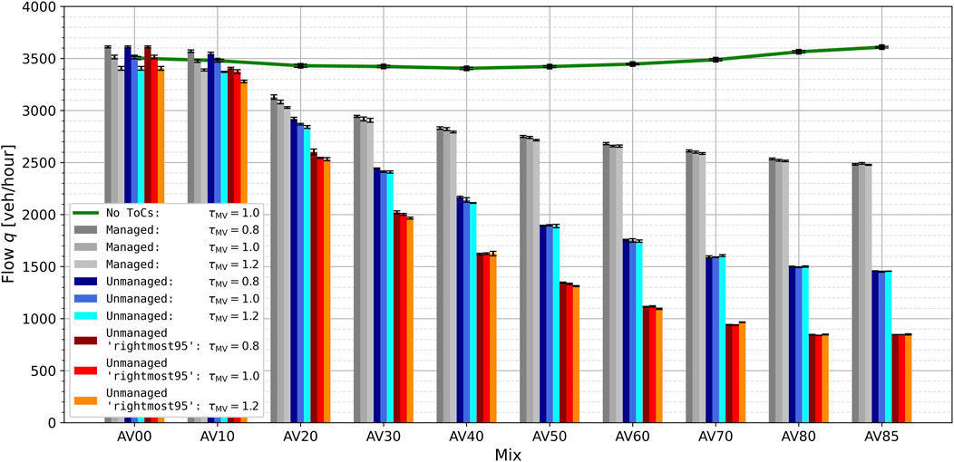
Figure 12. Maximum flow comparison across AV shares for the four scenarios: No ToCs (green line), Unmanaged ToCs (blue bars), Managed ToCs (gray bars), and Unmanaged “rightmost95” (red bars).

Overall, the results in Figure 12 show that in the unmanaged scenario, maximum flow declines significantly with increasing AV share. At AV85, the max flow is approximately $500\text{veh/h}$ lower than in the managed case—indicating that ToC management measures could help alleviate, but not fully prevent, capacity losses.

Furthermore, to compare these simulation results with the theoretical lane capacities estimated in Section 4.2 and Figure 10c, we derive the relative percentage reductions in capacity across the increasing AV share. Figure 13 summarizes these reductions for the unmanaged scenario, differentiating between the estimators max and mean, while constant is included as a reference that ignores ToC effects. For each estimator, we report the root mean squared error (RMSE) and the coefficient of determination (R²) to quantify the goodness of fit to the simulated capacity reductions—where lower RMSE and R² values closer to one indicate better agreement with the simulation data. The simulated results reveal a capacity loss of up to nearly 60% at AV85. We also make the following observations:

$•$ While the ${\tau }_{MV}$ dependency is relatively small in the simulation results, it becomes increasingly important in the estimator outcomes.

$•$ The notably poor performance of the constant estimator, including negative R² values in some cases, is expected since it does not capture capacity changes induced by ToCs.

$•$ Both estimators, max and mean, although accounting for ToCs, notably underestimate the capacity reductions in the mid-range AV share (AV20–80). This can be attributed to the simplicity of the numerical experiments we conducted to derive the estimator values. In particular, intensified vehicle interactions due to driver imperfections (parameter sigma $\sigma$) and speed factor variances are disregarded in these experiments. Additionally, the numerical experiments employ single-lane vehicle strings and uniform acceleration and deceleration parameters, omitting lane-changing interactions and parameter variability that are present in the two-lane simulation scenario (cf. Figure 5).

$•$ Compared to the ToC-ignorant estimator constant, the other estimators perform notably better in predicting ToC-related capacity reductions, particularly max, which achieves the best RMSE and R² scores. At AV85 share, max matches best with the simulation results, as vehicle interaction effects with non-AVs have almost completely vanished (still 15% HGVs present), leading to minimal driving behavior variability that coincides with the numerical experiment setup, where all vehicles share the same parameterization.

Figure 13

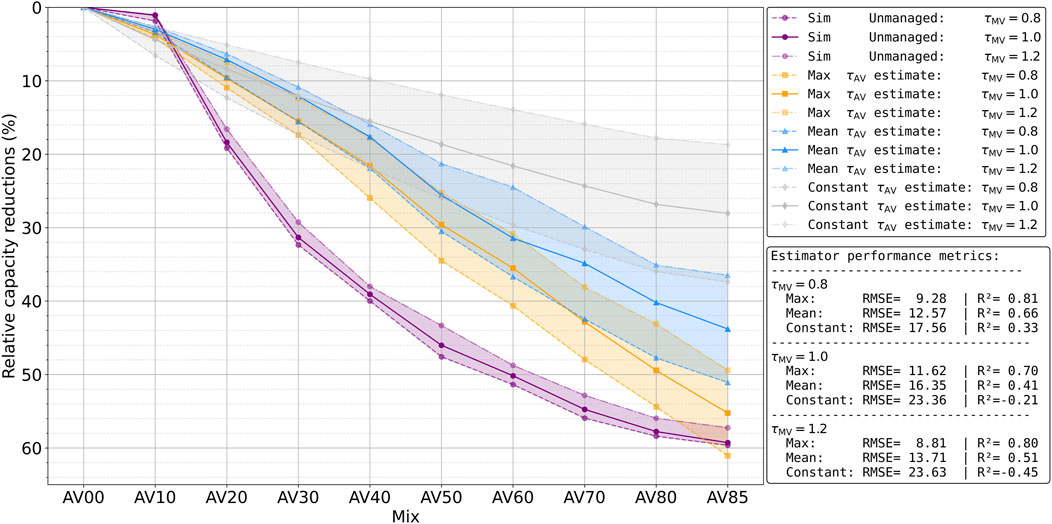
Figure 13. ToC-related relative percentage reductions of the capacity with varied mean ${\tau }_{MV}$-values for the unmanaged scenario. For reference, the estimator “constant” (gray-colored), which does not account for ToCs, is included. The RMSE and R² metrics indicate estimation accuracy.

In summation, the capacity reductions observed in the simulation might align only unsatisfactorily with theoretical estimates, as deviations occur in the mid-range AV shares due to the simplified assumptions of the estimators. This partial mismatch is also reflected in the RMSE and R² values, for which no established benchmarks exist in this context. Therefore, our assessment of estimator performance focuses on relative differences and qualitative trends within the observed results. However, the estimator max performs best in comparison to the simulation results, substantiating our suspicion that the maxima in time headway increments dominate ToC-related capacity effects. Nevertheless, the overall findings from Figures 12, 13 highlight the potential ToC effects on capacity reductions across various scenarios and parameter dependencies, in line with the stated expectations.

6 Conclusion

To investigate ToC-related capacity reductions, we conducted comprehensive simulation experiments with a calibrated two-lane highway scenario, as well as numerical experiments to estimate the large-scale impact of time headway increments during consecutive control transitions. Our main findings can be summarized as follows: (i) capacity reductions of up to $2000\text{veh/h}$, corresponding to approximately $60\%$ loss, were observed in shares with near-full Level 3 automation but no traffic management coordination; (ii) ToC effects became notably impactful starting from a Level 3 share of $10\%$ to $20\%$; (iii) a coordination of ToCs could mitigate losses by roughly $1000\text{veh/h}$ or $30\%$; (iv) binding Level 3 operation to the rightmost lane resulted in the most severe reduction, with up to $2660\text{veh/h}$ or $75\%$ loss; and (v) maxima in time headway increments during ToCs emerge as the dominant factor contributing to these capacity effects.

Several relevant limitations should be acknowledged, as they may affect the applicability and interpretation of our findings. Recent research on data from Level 4 AVs reveals reduced time headways when MVs follow AVs (Jiao et al., 2024). Such effects, which might also apply to Level 3 systems, are not considered in this study. An additional aspect that has not yet been discussed is the impact of human response times for non-emergency ToCs. Throughout this investigation, the response time distribution was kept the same, at $\mu =7\text{s}$ in all simulations, in line with our previous studies. More recent data from real-world tests presented by Pipkorn et al. (2023) indicate response times closer to 5 s, from which the authors infer that a lead time of $10\text{s}$, as specified in the R157, should be feasible for human drivers to take over in time. In our simulations, a few random sample reruns with these lower response times indicated approximately 10–$20\%$ higher capacities compared to the results presented here. A further limiting factor might be SUMO’s ACC model, which is parametrized for full string stability and deployed here as a proxy for Level 3 automated vehicles, although experimental studies and theoretical work have demonstrated string instabilities in ACC-equipped platoons, as we also discussed in Alms and Wagner (2024). All these limitations could potentially affect traffic capacity, though their precise contribution cannot be reliably quantified at this stage.

Future work should therefore include the development of a more accurate Level 3 model in SUMO, for example, an ACC-based ALKS system, as well as a systematic investigation of how model assumptions and human response variability together affect traffic capacity. Another important direction is to further examine the effects of MRMs, which are relevant for failed Level 3 transitions and Level 4 automation, on overall traffic, especially if they are not managed properly.

Lastly, we would like to reflect on the broader capacity implications of AVs. Our overall vehicle parametrization inherently results in slightly reduced theoretical capacities—even without ToCs—due to the implementation of lower time headways for MVs and higher ones for AVs, which contrasts with assumptions commonly made in other studies. While experimental research has demonstrated counterbalancing effects at high AV shares, which our own simulations also imply, this effect is diminished in the context of Level 3 systems. Unlike Level 4 or CACC-equipped vehicles, Level 3 automation, in its current form, does not typically support the low time headways often assumed to contribute to capacity gains. However, practical capacity impacts at relevant market penetration rates between 10% and 20% are likely still many years away, leaving room for further technical and regulatory development of Level 3 systems. Yet, in combination with the ToC-related capacity constraints demonstrated in this study, we take a more cautious view and do not share the seemingly widespread optimism regarding beneficial capacity effects of AVs in the mid-term.

Data availability statement

The raw data supporting the conclusion of this article will be made available by the authors, without undue reservation.

Author contributions

RA: Conceptualization, Data curation, Formal Analysis, Investigation, Methodology, Software, Validation, Visualization, Writing – original draft, Writing – review and editing. PW: Conceptualization, Methodology, Supervision, Writing – review and editing.

Funding

The author(s) declare that no financial support was received for the research and/or publication of this article.

Conflict of interest

The authors declare that the research was conducted in the absence of any commercial or financial relationships that could be construed as a potential conflict of interest.

Generative AI statement

The author(s) declare that no Generative AI was used in the creation of this manuscript.

Publisher’s note

All claims expressed in this article are solely those of the authors and do not necessarily represent those of their affiliated organizations, or those of the publisher, the editors and the reviewers. Any product that may be evaluated in this article, or claim that may be made by its manufacturer, is not guaranteed or endorsed by the publisher.

References

Alms, R., Noulis, A., Mintsis, E., Lücken, L., and Wagner, P. (2022). Reinforcement learning-based traffic control: mitigating the adverse impacts of control transitions. IEEE Open J. Intelligent Transp. Syst. 3, 187–198. doi:10.1109/OJITS.2022.3158688

CrossRef Full Text | Google Scholar

Alms, R., and Wagner, P. (2024). Control transitions in level 3 automation: safety implications in mixed-autonomy traffic. Safety 10, 1. doi:10.3390/safety10010001

CrossRef Full Text | Google Scholar

Alvarez Lopez, P., Banse, A., Barthauer, M., Behrisch, M., Couéraud, B., Erdmann, J., et al. (2025). Simulation of urban mobility (SUMO). doi:10.5281/zenodo.14796685

CrossRef Full Text | Google Scholar

Alvarez Lopez, P., Behrisch, M., Bieker-Walz, L., Erdmann, J., Flötteröd, Y.-P., Hilbrich, R., et al. (2018). “Microscopic traffic simulation using SUMO,” in The 21st IEEE International Conference on Intelligent Transportation systems (IEEE), 2575–2582.

Google Scholar

BASt (2021). Road Traffic Census Report 2021 - Ergebnisbericht der Straßenverkehrszählung 2021. Tech. rep. Fed. Highw. Res. Inst. (BASt).

Google Scholar

BASt (2025). Straßenverkehrszählung – verkehrsdatenbank.

Google Scholar

Bolovinou, A., Anagnostopoulou, C., Roungas, V., Amditis, A., González, R. B., Coello, L. T., et al. (2023). HI-DRIVE Deliverable D3.1/Use cases definition and description. Tech. Rep. Eur. Comm.

Google Scholar

Brilon, W., and Geistefeldt, J. (2010). Überprüfung der Bemessungswerte des HBS für Autobahnabschnitte außerhalb der Knotenpunkte, vol. 1033 of Forschung Straßenbau und Straßenverkehrstechnik. Bremerhaven, Germany: Wirtschaftsverl. NW Verl. für neue Wissenschaft.

Google Scholar

British Standards Institution (2020). PAS 1883:2020 - operational design domain (ODD) taxonomy for automated driving systems (ADS) – specification. London, UK: British Standards Institution.

Google Scholar

Calvert, S., and van Arem, B. (2020). A generic multi-level framework for microscopic traffic simulation with automated vehicles in mixed traffic. Transp. Res. Part C Emerg. Technol. 110, 291–311. doi:10.1016/j.trc.2019.11.019

CrossRef Full Text | Google Scholar

Digitale Plattform Stadtverkehr Berlin (2024). Verkehrsdetektion berlin.

Google Scholar

FGSV (2015). Handbuch für die Bemessung von Straßenverkehrsanlagen: HBS 2015. No. FGSV 299 B in FGSV W1 - Wissensdokumente (Cologne, Germany: FGSV-Verl). 2015 Edn.

Google Scholar

Friedrich, B. (2016). The effect of autonomous vehicles on traffic. Berlin, Heidelberg: Springer Berlin Heidelberg, 317–334. doi:10.1007/978-3-662-48847-8_16

CrossRef Full Text | Google Scholar

Geistefeldt, J., Giuliani, S., Busch, F., Schendzielorz, T., Haug, A., Vortisch, P., et al. (2017). “HBS-conform simulation of freeway traffic flow,” in vol. 279 of Berichte der Bundesanstalt für Straßen- und Verkehrswesen, Reihe V: Verkehrstechnik (Germany: Federal Highway Research Institute).

Google Scholar

Jiao, Y., Li, G., Calvert, S. C., van Cranenburgh, S., and van Lint, H. (2024). Beyond behavioural change: investigating alternative explanations for shorter time headways when human drivers follow automated vehicles. Transp. Res. Part C Emerg. Technol. 164, 104673. doi:10.1016/j.trc.2024.104673

CrossRef Full Text | Google Scholar

Kohanpour, E., Davoodi, S. R., and Shaaban, K. (2025). Trends in autonomous vehicle performance: a comprehensive study of disengagements and mileage. Future Transp. 5, 38. doi:10.3390/futuretransp5020038

CrossRef Full Text | Google Scholar

Liu, Q., Gao, C., Wang, H., Cai, Y., Chen, L., and Lv, C. (2024). Learning from trajectories: how heterogeneous CACC platoons affect the traffic flow in highway merging area. IEEE Trans. Veh. Technol. 73, 16212–16224. doi:10.1109/TVT.2024.3419143

CrossRef Full Text | Google Scholar

Lücken, L., Mintsis, E., Porfyri, K., Alms, R., Flötteröd, Y.-P., and Koutras, D. (2019). “From automated to manual - modeling control transitions with SUMO,”in SUMO user conference 2019. Editors M. Weber, L. Bieker-Walz, R. Hilbrich, and M. Behrisch (Stockport, United Kingdom: EPiC Series in Computing), 62, 124–144. doi:10.29007/sfgk

CrossRef Full Text | Google Scholar

Maerivoet, S., Akkermans, L., Carlier, K., Flötteröd, Y.-P., Lücken, L., Alms, R., et al. (2019). TransAID Deliverable 4.2 - preliminary simulation and assessment of enhanced traffic management measures. Tech. Rep. Eur. Comm.

Google Scholar

McDonald, A. D., Alambeigi, H., Engström, J., Markkula, G., Vogelpohl, T., Dunne, J., et al. (2019). Toward computational simulations of behavior during automated driving takeovers: a review of the empirical and modeling literature. Hum. Factors 61, 642–688. doi:10.1177/0018720819829572

PubMed Abstract | CrossRef Full Text | Google Scholar

Mercedes-Benz Group (2024). Mercedes-Benz is approved for 95 km/h Level 3 autonomous driving in Germany. Tech. Rep. Mercedes Benz Group.

Google Scholar

Mintsis, E., Koutras, D., Porfyri, K., Mitsakis, E., Lücken, L., Erdmann, J., et al. (2019). TransAID Deliverable 3.1 - modelling, simulation and assessment of vehicle automations and automated vehicles’ driver behaviour in mixed traffic. Tech. Rep. Eur. Comm.

Google Scholar

Park, J. E., Byun, W., Kim, Y., Ahn, H., and Shin, D. K. (2021). The impact of automated vehicles on traffic flow and road capacity on urban road networks. J. Adv. Transp. 2021, 1–10. doi:10.1155/2021/8404951

CrossRef Full Text | Google Scholar

Pipkorn, L., Tivesten, E., Flannagan, C., and Dozza, M. (2023). Driver response to take-over requests in real traffic. IEEE Trans. Human Mach. Syst. 53, 823–833. doi:10.1109/THMS.2023.3304003

CrossRef Full Text | Google Scholar

Rummel, J. (2017). Replication of the hbs autobahn with sumo. Berichte aus dem DLR-Institut für Verkehrssystemtechnik, Berlin, Germany: Institute of Transportation Systems, German Aerospace Center 171–178.

Google Scholar

SAE International (2021). SAE international recommended practice: taxonomy and definitions for terms related to driving automation systems for on-road motor vehicles. SAE Int. doi:10.4271/J3016_202104

CrossRef Full Text | Google Scholar

Sauvaget, J.-L., Dakil, M., Griffon, T., Anagnostopoulou, C., Bolovinou, A., Sintonen, H., et al. (2023). HI-DRIVE deliverable D5.1/descriptions of “operations”. Tech. Rep. Eur. Comm.

Google Scholar

Schrader, M. (2024). Calibrating traffic microsimulation for optimization of intelligent transportation systems using roadside radar. Tuscaloosa, AL: The University of Alabama. Ph.d. thesis.

Google Scholar

Schulte-Tigges, J., Matheis, D., Reke, M., Walter, T., and Kaszner, D. (2023). “Demonstrating a V2X enabled system for transition of control and minimum risk manoeuvre when leaving the operational design domain,” in HCI in mobility, transport, and automotive systems. Editor H. Krömker (Cham: Springer Nature Switzerland), 200–210. doi:10.1007/978-3-031-35678-0_12

CrossRef Full Text | Google Scholar

Shuttleworth, J. (2019). SAE updates J3016 automated-driving graphic. Mobil. Eng.

Google Scholar

TransAID (2021). Transition areas for infrastructure-assisted driving (TransAID). H2020 Res. Proj. 723390, Eur. Comm.

Google Scholar

UNECE (2023). Addendum 156 – UN regulation No. 157 - amendment 4 - uniform provisions concerning the approval of vehicles with regard to automated lane keeping systems. Tech. Rep. United Nations Economic commission for Europe.

Google Scholar

Van Aerde, M. (1995). “A single regime speed-flow-density relationship for freeways and arterials,” in 74th annual meeting of the transportation research board. Preprint paper no. 950802.

Google Scholar

Van Lint, J., and Calvert, S. C. (2018). A generic multi-level framework for microscopic traffic simulation—theory and an example case in modelling driver distraction. Transp. Res. Part B Methodol. 117, 63–86. doi:10.1016/j.trb.2018.08.009

CrossRef Full Text | Google Scholar

Wagner, P. (2012). Analyzing fluctuations in car-following. Transp. Res. Part B Methodol. 46, 1384–1392. doi:10.1016/j.trb.2012.06.007

CrossRef Full Text | Google Scholar

Wang, C., Ren, W., Xu, C., Zheng, N., Peng, C., and Tong, H. (2024). Exploring the impact of conditionally automated driving vehicles transferring control to human drivers on the stability of heterogeneous traffic flow. IEEE Trans. Intel. Veh., 1–17. doi:10.1109/TIV.2024.3419789

CrossRef Full Text | Google Scholar

Wang, C., Xu, C., Peng, C., Tong, H., Ren, W., and and, Y. J. (2025a). Predicting the duration of reduced driver performance during the automated driving takeover process. J. Intel. Transp. Syst. 29, 218–233. doi:10.1080/15472450.2024.2307029

CrossRef Full Text | Google Scholar

Wang, C., Xu, C., Shao, Y., Zheng, N., Peng, C., Tong, H., et al. (2025b). Identifying factors affecting driver takeover time and crash risk during the automated driving takeover process. J. Transp. Saf. Secur. 0, 1–26. doi:10.1080/19439962.2025.2450695

CrossRef Full Text | Google Scholar

Ward, T. (2024). “Areas of improvement for autonomous vehicles: a machine learning analysis of disengagement reports,” in 2024 International Conference on Electrics and Computer (INTCEC). ArXiv:2408.00051.

Google Scholar

Xiao, L., Wang, M., and van Arem, B. (2017). Realistic car-following models for microscopic simulation of adaptive and cooperative adaptive cruise control vehicles. Transp. Res. Rec. 2623, 1–9. doi:10.3141/2623-01

CrossRef Full Text | Google Scholar