 Yan Wang
 Rui Guo
 Lan Huang1
- 1Key Laboratory of Symbol Computation and Knowledge Engineering of Ministry of Education, and College of Computer Science and Technology, Jilin University, Changchun, China
- 2School of Artificial Intelligence, Jilin University, Changchun, China
N6-methyladenosine (m6A) is one of the most prevalent RNA post-transcriptional modifications and is involved in various vital biological processes such as mRNA splicing, exporting, stability, and so on. Identifying m6A sites contributes to understanding the functional mechanism and biological significance of m6A. The existing biological experimental methods for identifying m6A sites are time-consuming and costly. Thus, developing a high confidence computational method is significant to explore m6A intrinsic characters. In this study, we propose a predictor called m6AGE which utilizes sequence-derived and graph embedding features. To the best of our knowledge, our predictor is the first to combine sequence-derived features and graph embeddings for m6A site prediction. Comparison results show that our proposed predictor achieved the best performance compared with other predictors on four public datasets across three species. On the A101 dataset, our predictor outperformed 1.34% (accuracy), 0.0227 (Matthew’s correlation coefficient), 5.63% (specificity), and 0.0081 (AUC) than comparing predictors, which indicates that m6AGE is a useful tool for m6A site prediction. The source code of m6AGE is available at https://github.com/bokunoBike/m6AGE.
Introduction
N6-methyladenosine (m6A) is one of the most prevalent RNA post-transcriptional modifications. It was first found in mammalian RNA in 1974 (Desrosiers et al., 1974). Subsequently, m6A modification was observed in various species, such as Saccharomyces cerevisiae (Schwartz et al., 2013), Arabidopsis (Luo et al., 2014), humans and mouse (Dominissini et al., 2012). Research shows that m6A sites are enriched in long internal exons and 3′UTRs around stop codons rather than randomly distributed in the genome (Dominissini et al., 2012; Meyer et al., 2012; Wan et al., 2015). It has been reported that m6A modification is associated with many biological processes, including but not limited to protein translation and localization (Meyer and Jaffrey, 2014), mRNA splicing and stability (Nilsen, 2014), RNA localization and degradation (Meyer and Jaffrey, 2014). Therefore, precisely identifying m6A sites contributes to understanding the regulatory mechanism and biological significance of m6A modification.
High-throughput techniques have enabled locating the m6A sites in genomes. MeRIP-Seq (or m6A-Seq), a combination of immunoprecipitation and next-generation sequencing technology, has successfully mapped m6A in several species genomes (Dominissini et al., 2012; Schwartz et al., 2013; Wan et al., 2015). In 2015, Chenet al. developed photo-crosslinking-assisted m6A-sequencing (PA-m6A-seq) which provided a high-resolution (about 23nt) mammalian map (Chen et al., 2015a). MeRIP-Seq and PA-m6A-seq can only locate the high methylation regions of m6A rather than the exact positions. In the same year, Linder produced a single-nucleotide resolution map of m6A sites using a new technology termed miCLIP (Linder et al., 2015). However, the current experimental methods face a lot of limitations and expensive costs. With the rapid development of computational methods, it is possible to use machine learning algorithms to predict m6A. Hence, building advanced models to predict m6A sites is significant for the following research of m6A.
Chen et al. (2015b) proposed the first predictor named iRNA-Methyl for m6A sites in Saccharomyces cerevisiae, using three physical-chemical properties of dinucleotide and SVM classifier. WHISTLE (Chen et al., 2019) integrates genomic features besides the sequence features to train a predictor with SVM classifier. Liu and Chen (2020) developed a computational method called iMRM for detecting different RNA modifications simultaneously with XGBoost classifier. Recently, deep learning methods show better performance trend in bioinformatics problems. DeepM6ASeq (Zhang and Hamada, 2018), BERMP (Huang et al., 2018), Gene2vec (Zou et al., 2019), DeepPromise (Chen et al., 2020), and im6A-TS-CNN (Liu et al., 2020) establish deep learning frameworks by using convolutional neural network (CNN) layers and gated recurrent unit (GRU) to seek the m6A sites on DNA/RNA sequence level on the same dataset as SRAMP (Zhou et al., 2016). In this study, seven kinds of sequence-derived features are employed to encode RNA sequences, including CTD (Tong and Liu, 2019), Pseudo k-tuple Composition (PseKNC) (Guo et al., 2014), nucleotide pair spectrum (NPS) (Zhou et al., 2016), nucleotide pair position specificity (NPPS) (Xing et al., 2017), nucleotide chemical properties and density (NCP-ND) (Golam Bari et al., 2013), electron-ion interaction pseudopotentials (EIIP) (Nair and Sreenadhan, 2006), and bi-profile Bayes (BPB) (Shao et al., 2009). Besides, graph embedding methods are innovatively introduced to distill the potential structure information. Firstly, a network is constructed by mapping each sample of the dataset to a node. Secondly, the three graph embedding methods SocDim (Tang and Liu, 2009), Node2Vec (Grover and Leskovec, 2016), and GraRep (Cao et al., 2015) are used to learn the distributed representation of the sample in an unsupervised manner. At last, all the feature vectors are merged as the input of model. The predictive results show that m6AGE improves the performance of identifying m6A sites.
Materials and Methods
Datasets
The m6A sites of different species share different consensus motifs. The adenosines lying within the consensus motif are considered to be the potential methylation sites. The samples in the dataset are RNA sequence segments with the potential methylation sites at their center. The samples with the m6A sites experimentally annotated are put into the positive dataset, whereas the other samples are put into the negative dataset.
There have been many datasets across multiple species for training m6A site predictors. We have collected four datasets that involve three species: Saccharomyces cerevisiae, Arabidopsis thaliana, and human. The following are details of these datasets.
A101. Wang extracted A.thaliana m6A sites from the m6A peak data of Luo et al. (2014) and Wan et al. (2015). The dataset (Wang and Yan, 2018) Wang built contains 2,518 positive samples and 2,518 negative samples. Every sample in the dataset is a 101nt RNA sequence segment.
A25. Luo obtained 4,317 m6A peaks detected both in Can-0 and Hen-16 strains. After removing the sequences with more than 60% sequence similarity, Chen et al. (2016) obtained 394 positive samples. The same number of negative samples were selected randomly from sequences without the m6A site. The length of every sample is 25nt.
S21. Chen further constructed this dataset (Chen et al., 2015c) based on the previous work (Chen et al., 2015b). They selected 832 RNA sequence segments as the positive samples in the training set whose distances to the m6A-seq peaks are less than 10nt. Then, 832 of 33,280 RNA sequence segments with non-methylated adenines were selected randomly as negative samples in the training set. The rest 475 RNA sequences with methylated adenine and 4750 of 33,280 RNA sequences with non-methylated adenine constitute the independent testing dataset. The length of every sample is 21nt.
H41. Chen obtained the m6A-containing sequences in Homo sapiens from RMBase (Chen et al., 2017). All the m6A sites in these sequences conform to the RRACH motif. The dataset contains 1,130 positive samples and 1,130 negative samples. The length of every sample is 41nt.
Construction of Input Feature
Conventional machine learning models require numerical vectors as input features. The feature extraction methods selected have an important impact on the performance of the model. To fully characterize the context of m6A sites, seven sequence-derived features were used. In addition, we build a network based on the whole dataset, by mapping each sample to node and the similarity between samples to edges in the network, and then use graph embedding (neighborhood-based node embedding) methods to extract features in an unsupervised manner. The computational framework of our predictor is illustrated in Figure 1. In the following, we will introduce the sequence-derived features and the graph embeddings, respectively.
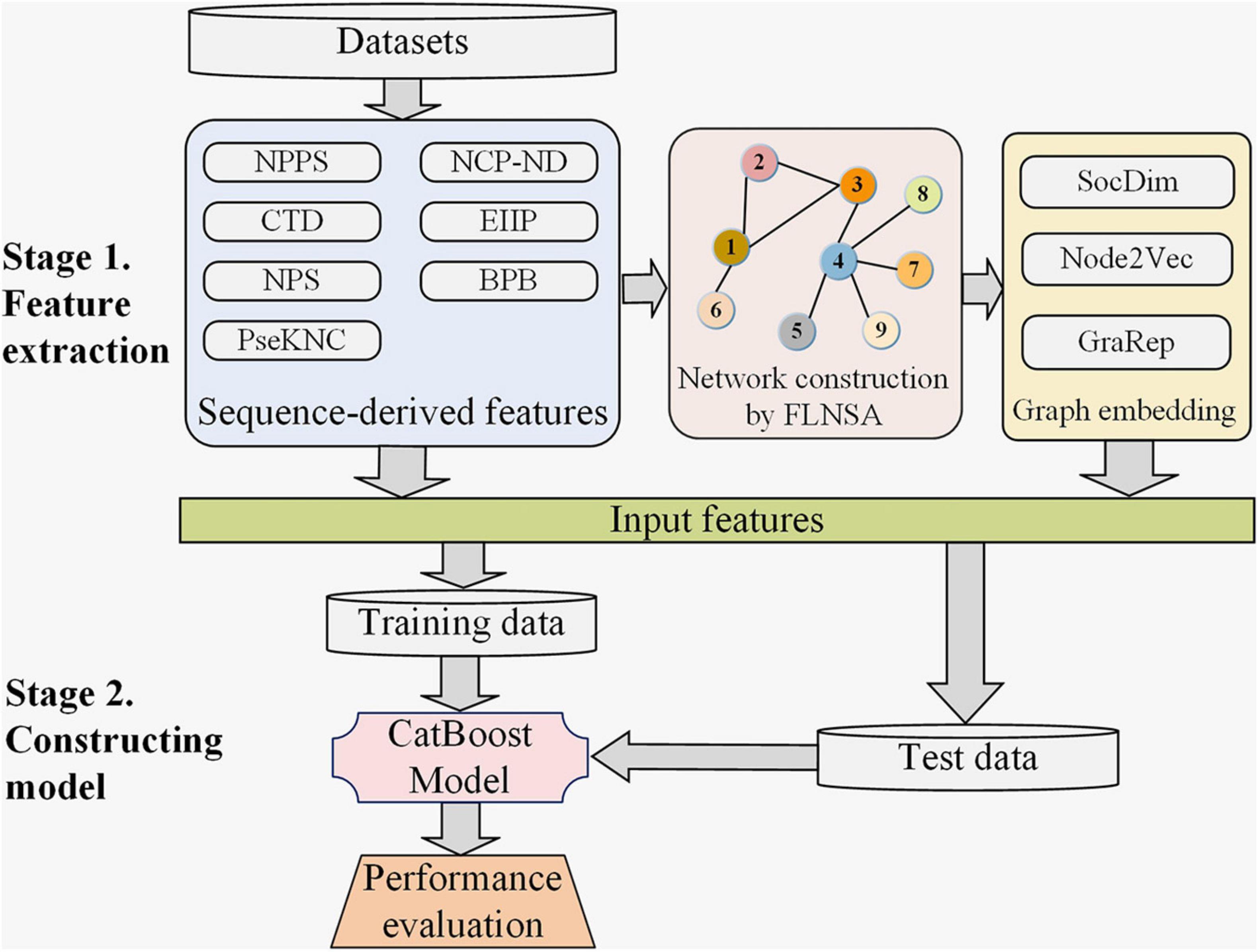
Figure 1. The computational framework of our predictor m6AGE. There are two main stages in the construction of m6AGE. Stage 1. Sequence-derived features are extracted, and graph embeddings are learned. Sequence-derived feature encoding methods directly encode RNA sequences into numerical vectors, including CTD, NPS, PseKNC, NPPS, NCP-ND, EIIP, and BPB feature encoding method. All the sequences are mapped to nodes of a network, and then their graph embeddings (SocDim, Node2Vec, and GraRep) are learned in an unsupervised manner. At last, the sequence features and graph embeddings are merged as input features. Stage 2. We divide the data into training data and test data with a ratio of 4:1. The training data is used to train a CatBoost model. The test data is used to evaluate the performance of our predictor.
Sequence-Derived Features
CTD Feature
CTD (Tong and Liu, 2019) is one of the global sequence descriptors. The first descriptor C (nucleotide composition) describes the percentage composition of each nucleotide in the sequence. The second descriptor T (nucleotide transition) describes the frequency of four different nucleotides present in adjacent positions. The third descriptor D (nucleotide distribution) describes five relative positions of each nucleotide along the RNA sequence which are the first one, 25%, 50%, 75%, and the last one.
PseKNC Feature
With the successful application of the pseudo component method in peptide sequence processing, its idea has been further extended to the study of DNA and RNA sequences feature representation. The Pseudo k-tuple Composition (PseKNC) combines the local and global sequence information of RNA (Guo et al., 2014) and transforms an RNA sequence into the following vector:
where,
where du(u = 1,2,…,4k) is the occurrence frequency of the u-th k-nucleotide in this RNA sequence; the parameter w is the weight factor; the parameter λ is the number of totals counted tiers of the correlations along an RNA sequence. The j-tier correlation factor θj is defined as follows:
The correlation function Θ(,) is calculated by the following formula:
where μ is the number of RNA physicochemical properties used. RiRi+1 is the dinucleotide at position i of this RNA. Pν(RiRi + 1) is the standardized numerical value of the ν-th RNA physicochemical properties for dinucleotide RiRi +1.
Six RNA physicochemical properties are considered: “Rise”, “Roll”, “Shift”, “Slide”, “Tilt”, “Twist”.
NPS Feature
The nucleotide pair spectrum (NPS) (Zhou et al., 2016) encoding method describes the RNA sequence context of the site by calculating the occurrence frequency of all k-spaced nucleotide pairs in the sequence. The k-spaced nucleotide pair n1{k}n2 means that there are k arbitrary nucleotides between n1 and n2, and its occurrence frequency is calculated as follows:
where C(n1{k}n2) is the count of n1{k}n2 in this RNA sequence, and L is the sequence length. The parameter k ranges from 1 to dmax. The parameter dmax is set to 3, so this encoding method transforms an RNA sequence into a vector DNPS with a dimension of 4×4×3=48.
NPPS Feature
The nucleotide pair position specificity (NPPS) (Xing et al., 2017) encoding method extracts statistical information by calculating the frequency of single nucleotide and k-spaced nucleotide pairs at specific locations. Based on the positive training dataset, we can get the frequency matrix
where the element of is the frequency of single nucleotide appearing at each location in the positive training dataset; the element of is the frequency of k-spaced nucleotide pair appearing at each location in the positive training dataset; and L is the sequence length. The frequency matrix and are calculated similarly on the negative training dataset.
Assuming that the i-th nucleotide is “A” and the (i + k)-th nucleotide is “C”, is calculated through conditional probability formula and frequency matrix:
NPPS encoding method transforms a sequence into a vector DNPPS=[pk + 2,…,pL] with a dimension of L−k−1, where .
NCP-ND Feature
Different nucleotides have different chemical properties. According to the difference of ring structure (purine or pyrimidine), hydrogen bond (strong or weak), and functional group (amino or keto), nucleotide A, U, C, and G can be represented by (1, 1, 1), (0, 1, 0), (0, 0, 1), and (1, 0, 0), respectively (Golam Bari et al., 2013).
The nucleotide density (ND) is used to measure the relevance between the frequency and position of the i-th nucleotide ni in the sequence:
where L is the sequence length. Combined with the chemical properties of nucleotides, each sequence is transformed into a vector DNCP−ND with a dimension of L×4.
EIIP Feature
This encoding method uses the electron-ion interaction pseudopotentials (EIIP) values (Nair and Sreenadhan, 2006) to represent the nucleotide in the sequence. The EIIP values of nucleotides A, T (we replace T with U), C, G are 0.1260, 0.1340, 0.0806, and 0.1335, respectively. Thus the dimension of the vector DEIIP is equal to the sequence length.
BPB Feature
The Bi-profile Bayes (BPB) encoding method was first proposed by (Shao et al., 2009), and then has been successfully applied in other fields of bioinformatics. This method uses the occurrence frequency fi,n of the i-th nucleotide n to estimate the posterior probability pi,n, and transforms a sequence into the following vector:
where n is the i-th nucleotide of the sequence; denotes the frequency of nucleotide n appearing at the i-th position of the sequence in the positive training dataset, while denotes the frequency of nucleotide n appearing at the i-th position of sequence in the negative training dataset. L is the sequence length. The dimension of the vector DBPB is 2×L.
Graph Embeddings
Network Construction
To extract the graph embedding feature of each sample, we construct a network based on the whole dataset. Each sample in the dataset is taken as a node, and the relationships between samples are taken as edges. Generally, edges exist two similar sample nodes. The fast linear neighbor similarity approach (FLNSA) (Zhang et al., 2017, 2019) is a method to extract “sample-sample” similarity, which has been successfully applied to many bioinformatics classification tasks. In this study, FLNSA is utilized to calculate the similarity between samples.
First, we extract sequence-derived features and use the feature fusion strategy to transform all the samples in the dataset into n-dimensional vector {x1,x2,…,xm}, where xi(0 < i≤m) is the vector of the i-th sample. Then these vectors are concentrated into a matrix X ∈ Rm×n, each row of which represents a sample vector. FLNSA tries to minimize the objective function:
where ⊙ is the Hadamard product operator; ||⋅||F represents the Frobenius norm and μ is the regularization coefficient. e is an m-dimensional column vector with all elements equal to 1. The element wi,j of matrix W ∈ Rm×m represents the reconstruction contribution weight of the sample xj to the sample xi, and is used to quantify the similarity between two samples. The element of indicator C ∈ Rm×m is
where N(xi) denotes the set of all neighbors of xi. The Euclidean distances between xi and other samples are calculated and the nearest c(0 < c < m) samples are selected to form N(xi). FLNSA uses the Lagrange method to get matrix W. After mathematical derivation, the Equation (13) is obtained.
Randomly generated matrix W was updated according to Equation (13) until convergence. Taking W as the adjacency matrix, an undirected weighted graph G is obtained. The graph embedding methods require a connected graph as input. Note that if G is not connected, we can increase c (the number of neighborhoods of a sample). Under the condition of ensuring the connectivity of the graph, the edges whose weights are lower than the threshold t are removed and the weights of the remaining edges are set to 1. Finally, an undirected unweighted graph is constructed based on the dataset.
SocDim
The social-dimension-based (SocDim) (Tang and Liu, 2009) method is proposed by Lei Tang and Huan Liu to solve the relational learning between nodes in social networks. This method extracts latent dimensions from networks and uses them as distributed representations, which involves community detection tasks.
SocDim uses Modularity (Newman, 2006) which measures community structure through degree distribution to extract potential dimensions. Modularity considers dividing the network into non-overlapping communities, measures the deviation between the network and uniform random graphs with the same degree distribution, and then obtains the modularity matrix B defined as follows:
where A is the interaction matrix of the network; d is a column vector composed of the degrees of each node; m is the number of nodes. Subsequently, SocioDim extracts the dimensions from the top eigenvectors of the modularity matrix B.
Node2Vec
Node2Vec (Grover and Leskovec, 2016) attempts to design a graph embedding model that can train efficiently and retain the neighborhood information of nodes to the maximum extent. The embedding vectors of nodes are learned through the skip-gram model. Different from DeepWalk, Node2Vec proposes biased random walk instead of truncated random walk to control the search space. Node2vec considers the homophily (nodes from the same community have similar embeddings) and structural equivalence (nodes that share similar roles have similar embeddings), thus there are two classic search strategies: Breadth-first Sampling (BFS) and Depth-first Sampling (DFS).
GraRep
GraRep (Cao et al., 2015) proposes a graph embedding model that can be learned from weighted graphs and integrate global structure information of the graph. GraRep forms k different vectors by separating k kinds of relationships. For a specific k, GraRep samples a set of k-step paths from the graph. The k-step path which starts with node vw and ends with node vc is denoted as (vw,vc). For all pairs, it increases the probability of the pairs come from the graph and decreases the probability of the pairs do not come from the graph. Based on the normalized adjacency matrix, GraRep obtains Wk for different values of k, and each column vector of Wk represents an embedding of the node. Finally, this method concatenates all the k-step representations W1,W2,…,Wk.
CatBoost Classifier
CatBoost (Dorogush et al., 2018; Prokhorenkova et al., 2018) is an improved implementation of gradient enhanced decision trees (GDBT) algorithm developed by Yandex. It has demonstrated excellent performance on many classification and regression tasks. Compared with other advanced gradient boosting algorithms such as XGBoost (Chen and Guestrin, 2016) and lightBGM (Ke et al., 2017), CatBoost has the following advantages: (1) It can better process categorical features. (2) To solve the problem of gradient bias and prediction shift, ordered boosting is proposed instead of the classic GDBT gradient estimation algorithm. (3) The requirement of super parameter tuning is reduced.
CatBoost uses oblivious decision trees (Langley and Sage, 1994) as base predictors. As oblivious decision trees are balanced, they can prevent overfitting. Moreover, it optimizes the traditional boosting algorithm which transforms the category features into numerical features, and the algorithm of calculating the leaf value to improve the generalization ability of the model. Since the CatBoost algorithm is running on GPU, the model is trained efficiently and parallelly.
Evaluation Metrics
Our predictor predicts whether the adenosine at the center of an RNA sequence segment is an m6A site. We used the following metrics to evaluate the performance of binary classification predictors: accuracy (ACC), Matthew’s correlation coefficient (MCC), sensitivity (SEN), specificity (SPE), and F1. These metrics are calculated as follows:
where TP is the number of true positive samples; TN is the number of true negative samples; FP is the number of false positive samples; FN is the number of false negative samples.
Additionally, the receiver operating characteristic (ROC) curve is also an important measurement to evaluate the performance of classifiers, and the area under receiver operating characteristic curve (AUC) is the quantitative indicator. High values of AUC indicate better performance of predictors.
Results
We redivided the four datasets introduced in section “Datasets” into the training sets and test sets with the ratio of 4:1, respectively. The training datasets were used to train models and the test datasets were utilized to evaluate model performance. Due to the difference between datasets, we selected suitable sequence-derived features for each dataset. For A101, the PseKNC, CTD, and NPS features were selected; For A25, the EIIP, NPPS, NPS, PseKNC, and NCP-ND were selected; For S21, the NPPS and NCP-ND features were selected; For H41, the NCP-ND, PseKNC, and NPPS features were selected.
Comparison With Existing Predictors
In this section, we compared the performance of our predictor m6AGE with several other state-of-the-art predictors, including M6A-HPCS (Zhang et al., 2016), Targetm6A(Li et al., 2016), RAM-NPPS (Xing et al., 2017), M6APred-EL (Wei et al., 2018), and DeepM6ASeq (Zhang and Hamada, 2018). M6A-HPCS uses PseDNC and DACC features and a support vector machine (SVM) classifier to identify m6A sites. Targetm6A utilizes position-specific kmer propensities (PSKP) feature and SVM classifier. RAM-NPPS uses the NPPS feature and SVM classifier to identify m6A sites. M6APred-EL creates an ensemble model with PseKNC, PSKP, and NCP-ND features. DeepM6ASeq develops a deep learning framework and uses one-hot encoding for the identification of m6A sites. The predictor M6A-HPCS, M6APred-EL, Targetm6A, and RAM-NPPS were reproduced faithfully, and their parameters were optimized by grid search with five-fold cross-validation. All predictors were trained and evaluated on the same dataset for fairness of comparison.
The evaluation results were summarized in Table 1. We employed ACC, MCC, SEN, SPE, and AUC as evaluation metrics, and compared the evaluation metrics of m6AGE with five other predictors on three datasets: A101, A25, and H41. As shown in Table 1, our predictor m6AGE achieved all optimal values on three datasets, except for SEN and SPE on the A25 dataset, and AUC on the H41 dataset.
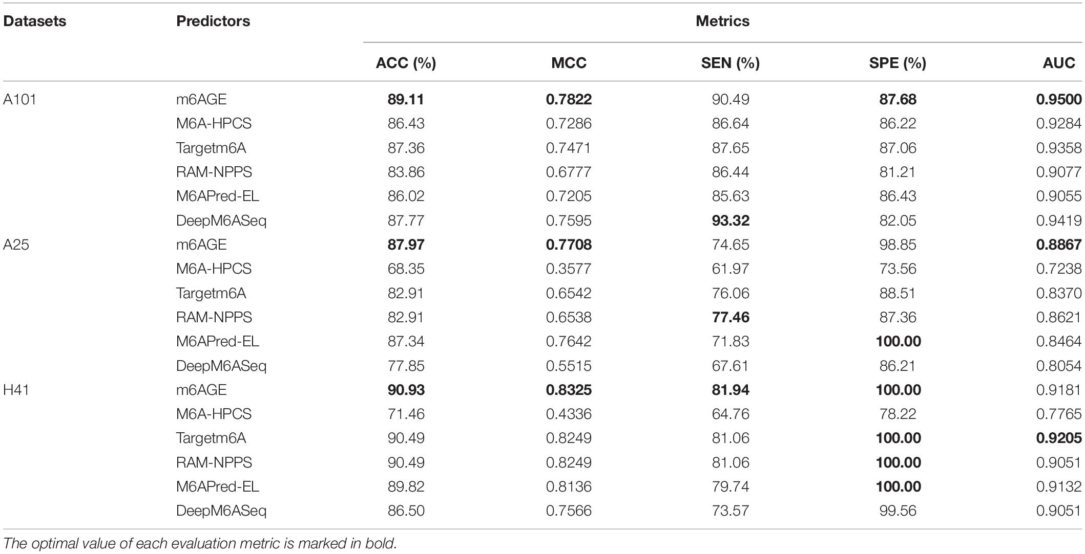
Table 1. The performance of m6AGE against other existing predictors.
On the A101 dataset, m6AGE obtained the optimal ACC, MCC, SPE, and AUC with 89.11%, 0.7822, 87.68%, and 0.9500, which is 1.34%, 0.0227, 5.63%, and 0.0081 higher than the suboptimal predictor DeepM6ASeq, respectively.
On the A25 dataset, m6AGE obtained the optimal ACC, MCC, and AUC with 87.97%, 0.7708, and 0.8867. Its Acc and MCC is 0.63% and 0.0066 higher than the suboptimal value of predictor M6APred-EL. Its AUC is 0.0246 higher than the suboptimal value of predictor RAM-NPPS.
On the H41 dataset, m6AGE obtained the optimal ACC, MCC, SEN, and SPE with 90.93%, 0.8325, 81.94%, and 100%, which is 0.44%, 0.0076, 0.88%, and 0 higher than the predictor Targetm6A and RAM-NPPS, respectively.
The ROC curves of these predictors on three datasets were plotted in Figure 2. As shown in Figure 2, our predictor outperformed other predictors on the A101 and A25 datasets. Although the AUC of m6AGE on dataset H41 is lower than other predictors, m6AGE achieved the optimal value of ACC, MCC, SEN, and SPE. These evaluation results demonstrate that our predictor m6AGE is superior to other predictors in terms of these three datasets.
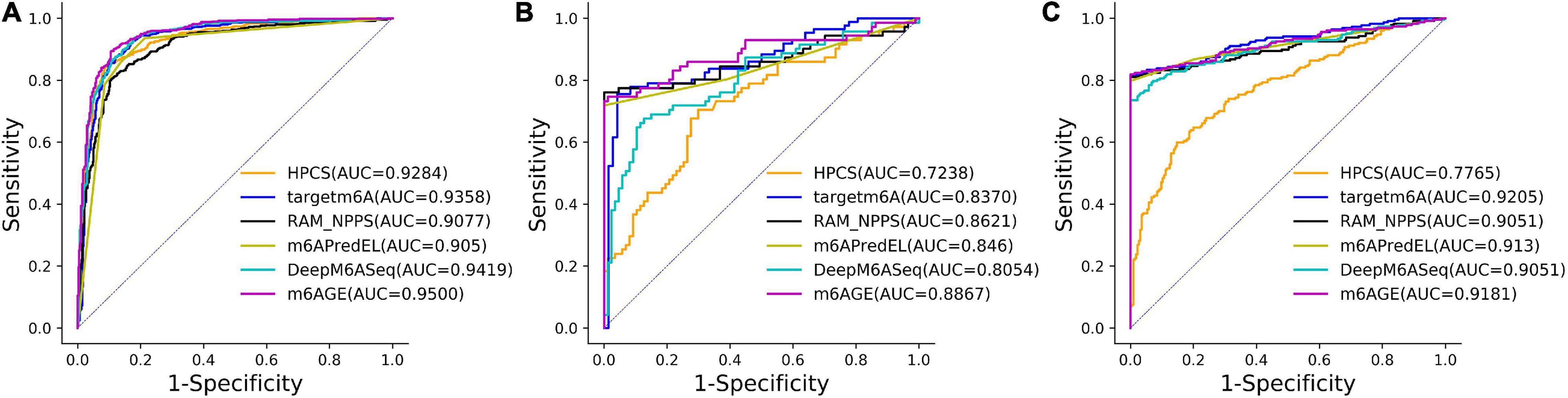
Figure 2. The ROC curves of m6AGE and comparing predictors on three datasets. (A) The ROC curves on the A101 dataset. (B) The ROC curves on the A25 dataset. (C) The ROC curves on the H41 dataset.
Performance on Imbalanced Dataset
The non-m6a sites on mRNA are much more than m6A sites, so testing the performance of our predictor on imbalanced datasets is of great importance. The imbalance ratio of the S21 dataset is about 1:4. We redivided the S21 dataset, and randomly selected 80% samples as the training set, and the remaining 20% samples as the test set.
CatBoost solves the imbalance data issues by setting weights for each class or sample. The weight of each class is generally inversely proportional to the number of its samples. The metrics F1 and MCC are usually used as the evaluation criteria for imbalanced datasets (Zhao et al., 2018; Wang et al., 2019; Dou et al., 2020). We compared m6AGE with five other predictors on the S21 dataset.
The evaluation results were summarized in Table 2. The optimal value of each evaluation metric is marked in bold. As shown in Table 2, our predictor m6AGE got the optimal values of F1, MCC, and AUC with 0.5723, 0.4593, and 0.8103.
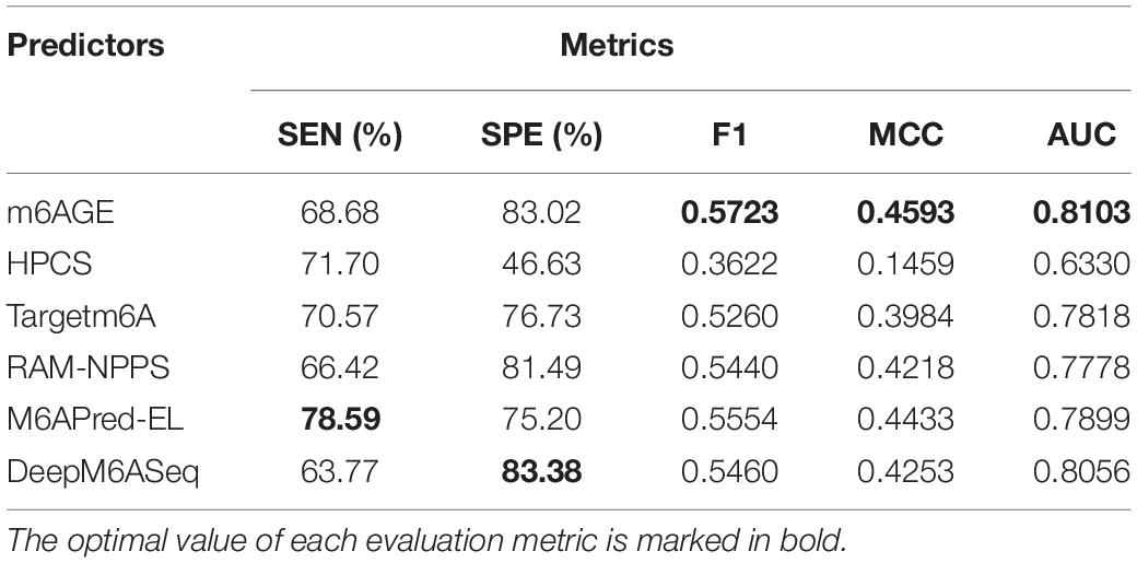
Table 2. The performance of different predictors on S21 dataset.
The ROC curves of these predictors on the S21 dataset were plotted in Figure 3. As shown in Figure 3, our predictor outperformed other predictors on the S21 dataset.
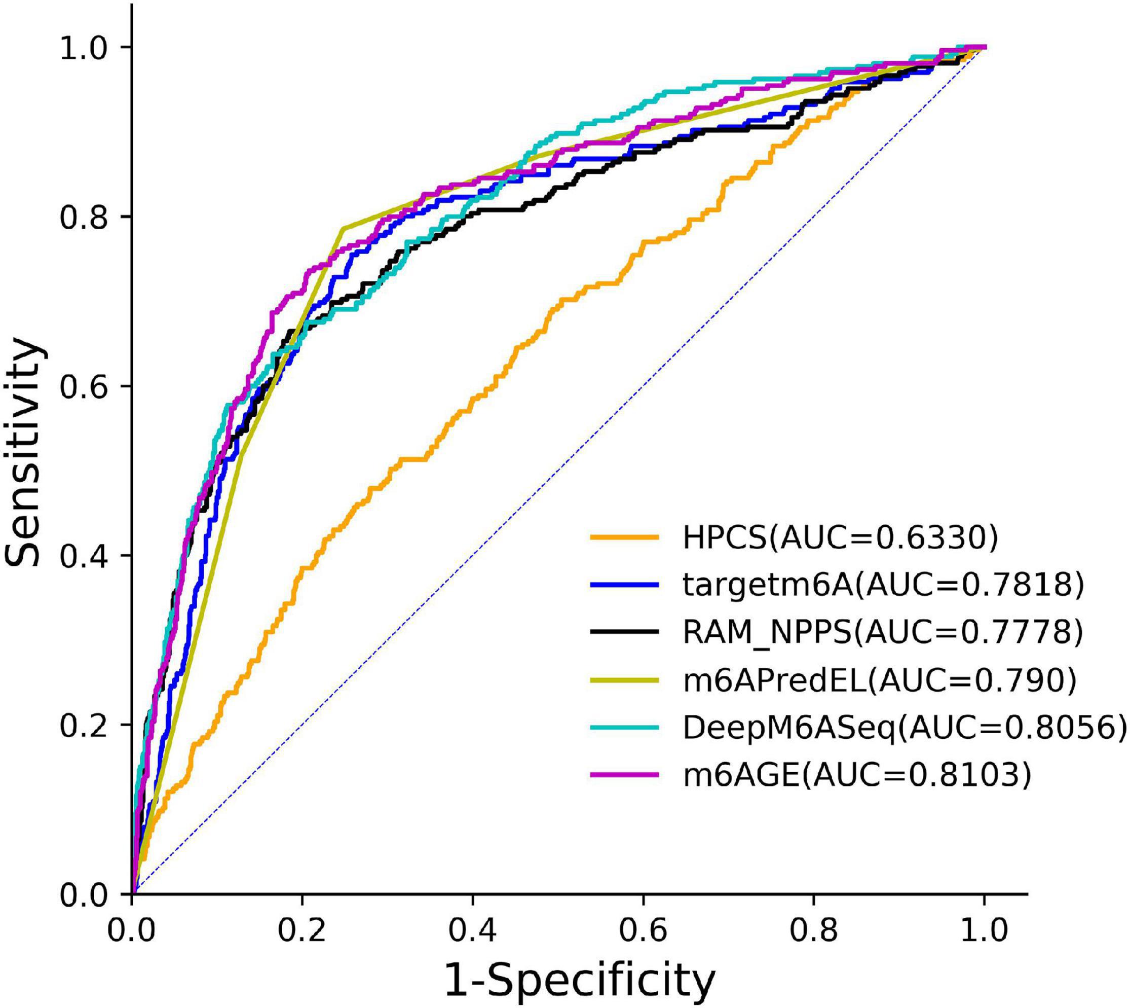
Figure 3. The ROC curves of m6AGE and comparing predictors on the S21 datasets.
Comparison With Different Classifiers
To further demonstrate the effectiveness of CatBoost, we compared it with other popular classifiers, including Random Forest, Logistic Regression, and Decision Tree, which are commonly and widely used in bioinformatics classification tasks. All classifiers were trained and assessed under the same conditions for a fair comparison.
The prediction results were summarized in Table 3. We compared the prediction results with three other classifiers on the A101, A25, and H41 dataset. The evaluation metrics used are ACC, MCC, SEN, SPE, and AUC. As shown in Table 3, CatBoost achieved all optimal metrics on three datasets, except for SPE on the A101 dataset and SEN on the A25 and H41 dataset.
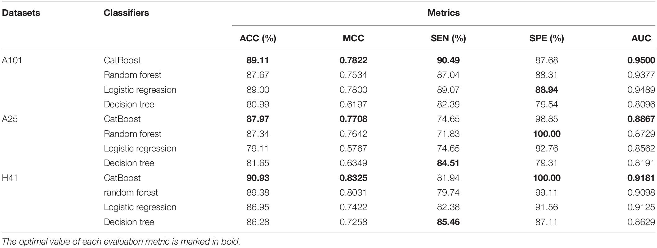
Table 3. The performance of different classifiers.
Feature Importance Analysis
CatBoost can output the scores of feature importance, which reflect the contributions of the features in specific feature space for identifying m6A sites. The first 20 important features and their scores on the four datasets were plotted in Figure 4.
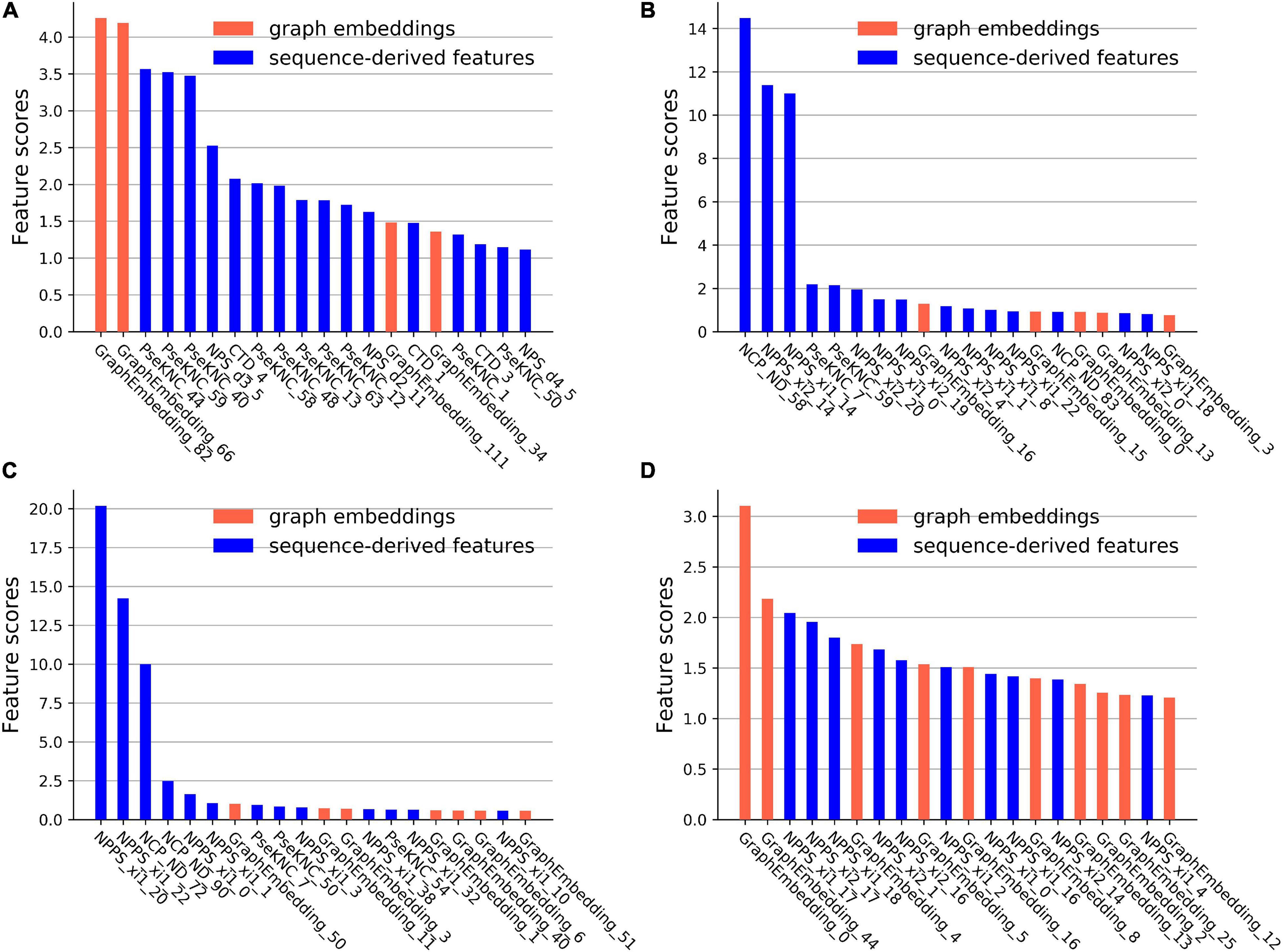
Figure 4. The feature importance scores on the four datasets. (A) The feature importance scores on the A101 datasets. (B) The feature importance scores on the A25 datasets. (C) The feature importance scores on the H41 datasets. (D) The feature importance scores on the S21 datasets.
On the A101 dataset, the first three important sequence-derived features are “PseKNC_44”, “PseKNC_59”, and “PseKNC_40”, which correspond to the occurrence frequency of “GUA”, “UGU”, and PseKNC_40 respectively, On the A25 dataset, the first three important sequence-derived features are “NCP_ND_58”, “NPPS_xi2_14”, and “NPPS_xi1_14,” which correspond to the position +1 (Assuming that the position of m6A site is 0), +2 and +4, +2 and +3, respectively; On the H41 dataset, the first three important sequence-derived features are “NPPS_xi1_20”, “NPPS_xi1_22”, and “NCP_ND_72”, which correspond to the position 0 and +1, +2 and +3, −3, respectively; On the S21 dataset, the first three important sequence-derived features are “NPPS_xi1_17”, “NPPS_xi2_17”, and “NPPS_xi1_18,” which correspond to the position +6 and +7, +6 and +8, +7 and +9, respectively.
In addition, graph embeddings account for 20%, 25%, 35%, and 50% of the top 20 important features in the four datasets, respectively, which indicates that graph embeddings could supplement the information of the sequence-derived features.
Discussion
The methods for extracting sequence features are indispensable for building a reliable predictor. Contributing sequence features, such as the physical and chemical properties of nucleotides, the frequency of k-nucleotides, and the frequency of specific positions, can fully reflect the information related to the m6A site recognition. In this study, we integrated and selected suitable sequence-derived features for each dataset. However, most of the feature encoding methods are based on the primary sequence, and only a few of them calculate the frequency of nucleotides in the training dataset, so it is difficult to obtain more helpful information from the whole dataset. This paper innovatively introduces a feature extraction method based on the graph embedding methods as a supplement to sequence-derived features. First of all, a network is constructed based on the whole dataset and sequence-derived features. Samples are abstracted as nodes of the network, and the similarity relationships between samples are abstracted as edges. This network reflects global information of the whole dataset. Then, graph embedding (neighborhood-based node embedding) methods are used to learn the feature representation of each node in an unsupervised manner. The graph embedding features of samples contain the related information with other samples. Finally, we integrate sequence-derived features and graph embeddings based with the feature fusion strategy. Therefore, the final input features can reflect the information of samples more comprehensively.
It is also significant to choose an appropriate classifier. CatBoost is a GBDT algorithm, which shows excellent performance in many classification tasks. Because of its good effect of restraining overfitting and fast running, the CatBoost algorithm is selected to train our predictor m6AGE.
To further prove the effectiveness of our predictor, we compare the evaluation results with that of other existing m6A site predictors. The results show that our predictor m6AGE outperforms other existing methods. In the future, we will apply m6AGE to more m6A site datasets and seek more suitable graph embedding methods. It is worth mentioning that the computational framework proposed in this study is possible to extend to other bioinformatics site identification tasks.
The source code of m6AGE is available at https://github.com/bokunoBike/m6AGE. Users can download and run it on the local machines. The data is imported through the file paths of the positive training set, negative training set, and test set. Then m6AGE is trained and generates prediction results. Note that the corresponding python packages need to be installed first (see GitHub page for details). For a new dataset, our predictor will automatically select the appropriate sequence-derived features (or specified by the users in the corresponding configuration file) according to the feature importance scores.
Conclusion
The identification of N6-methyladenosine (m6A) modification sites on RNA is of biological significance. In this study, a novel computational framework called “m6AGE” is proposed to predict and identify the m6A sites on mRNA. Our predictor combines sequence-derived features with the features extracted by graph embedding methods. The context information of sites is directly extracted from primary sequences by the sequence-derived features, and the global information is extracted by the graph embeddings. Experiments showed that the proposed m6AGE achieved successful prediction performance on four datasets across three species. It could be expected that m6AGE would be a powerful computational tool for predicting and identifying the m6A modification sites on mRNA.
Data Availability Statement
Publicly available datasets were analyzed in this study. Codes and data are available here: https://github.com/bokunoBike/m6AGE which contains detailed steps to run m6AGE.
Author Contributions
YW and RG conceived the algorithm and developed the program. RG, YW, and SY wrote the manuscript and prepared the datasets. YW and SY helped with manuscript editing, design. XMH, LH, and KH helped to revise the manuscript. All authors contributed to the article and approved the submitted version.
Funding
This work was supported by the National Natural Science Foundation of China (No. 62072212), the Development Project of Jilin Province of China (Nos. 20200401083GX, 2020C003), and Guangdong Key Project for Applied Fundamental Research (No.2018KZDXM076). This work was also supported by Jilin Province Key Laboratory of Big Data Intelligent Computing (No. 20180622002JC).
Conflict of Interest
The authors declare that the research was conducted in the absence of any commercial or financial relationships that could be construed as a potential conflict of interest.
References
Cao, S., Lu, W., and Xu, Q. (2015). “GraRep: learning graph representations with global structural information,” in Proceedings of the 24th ACM International on Conference on Information and Knowledge Management, (New York, NY:Association for Computing Machinery), 891–900. doi: 10.1145/2806416.2806512
Chen, T., and Guestrin, C. (2016). “XGBoost: a scalable tree boosting system,” in Proceedings of the 22nd ACM SIGKDD International Conference on Knowledge Discovery and Data Mining, (New York, NY:Association for Computing Machinery), 785–794. doi: 10.1145/2939672.2939785
Chen, K., Lu, Z., Wang, X., Fu, Y., Luo, G.-Z., Liu, N., et al. (2015a). High-Resolution N 6 -methyladenosine (m 6 A) map using photo-crosslinking-assisted m 6 a sequencing. Angew. Chemie127, 1607–1610. doi: 10.1002/ange.201410647
Chen, W., Feng, P., Ding, H., Lin, H., and Chou, K. C. (2015b). IRNA-Methyl: identifying N6-methyladenosine sites using pseudo nucleotide composition. Anal. Biochem.490, 26–33. doi: 10.1016/j.ab.2015.08.021
Chen, W., Feng, P., Ding, H., and Lin, H. (2016). Identifying N 6-methyladenosine sites in the Arabidopsis thaliana transcriptome. Mol. Genet. Genomics291, 2225–2229. doi: 10.1007/s00438-016-1243-7
Chen, W., Tang, H., and Lin, H. (2017). MethyRNA : a web server for identification of N–methyladenosine sites. J. Biomol. Struct. Dyn.1102, 1–5. doi: 10.1080/07391102.2016.1157761
Chen, W., Tran, H., Liang, Z., Lin, H., and Zhang, L. (2015c). Identification and analysis of the N6-methyladenosine in the Saccharomyces cerevisiae transcriptome. Sci. Rep.5:13859. doi: 10.1038/srep13859
Chen, K., Wei, Z., Zhang, Q., Wu, X., Rong, R., Lu, Z., et al. (2019). WHISTLE: a high-accuracy map of the human N6-methyladenosine (m6A) epitranscriptome predicted using a machine learning approach. Nucleic Acids Res.47:e41. doi: 10.1093/nar/gkz074
Chen, Z., Zhao, P., Li, F., Wang, Y., Smith, A. I., Webb, G. I., et al. (2020). Comprehensive review and assessment of computational methods for predicting RNA post-transcriptional modification sites from RNA sequences. Brief. Bioinform.21, 1676–1696. doi: 10.1093/bib/bbz112
Desrosiers, R., Friderici, K., and Rottman, F. (1974). Identification of methylated nucleosides in messenger RNA from novikoff hepatoma cells. Proc. Natl. Acad. Sci. U.S.A.71, 3971L–3975. doi: 10.1073/pnas.71.10.3971
Dominissini, D., Moshitch-Moshkovitz, S., Schwartz, S., Salmon-Divon, M., Ungar, L., Osenberg, S., et al. (2012). Topology of the human and mouse m6A RNA methylomes revealed by m6A-seq. Nature485, 201–206. doi: 10.1038/nature11112
Dorogush, A. V., Ershov, V., and Gulin, A. (2018). CatBoost: gradient boosting with categorical features support. arXiv [Preprint]arXiv:1810.11363,Google Scholar
Dou, L., Li, X., Ding, H., Xu, L., and Xiang, H. (2020). IRNA-m5C_NB: a novel predictor to identify RNA 5-methylcytosine sites based on the naive bayes classifier. IEEE Access8, 84906–84917. doi: 10.1109/ACCESS.2020.2991477
Golam Bari, A. T. M., Reaz, M. R., Choi, H. J., and Jeong, B. S. (2013). “DNA encoding for splice site prediction in large DNA sequence,” in Database Systems for Advanced Applications.DASFAA 2013. Lecture Notes in Computer Science, Vol. 7827, eds B.Hong, X.Meng, L.Chen, W.Winiwarter, and W.Song (Berlin: Springer), doi: 10.1007/978-3-642-40270-8_4
Grover, A., and Leskovec, J. (2016). “Node2vec: scalable feature learning for networks,” in Proceedings of the 22nd ACM SIGKDD International Conference on Knowledge Discovery and Data Mining, (New York, NY:Association for Computing Machinery), 855–864. doi: 10.1145/2939672.2939754
Guo, S. H., Deng, E. Z., Xu, L. Q., Ding, H., Lin, H., Chen, W., et al. (2014). INuc-PseKNC: a sequence-based predictor for predicting nucleosome positioning in genomes with pseudo k-tuple nucleotide composition. Bioinformatics30, 1522–1529. doi: 10.1093/bioinformatics/btu083
Huang, Y., He, N., Chen, Y., Chen, Z., and Li, L. (2018). BERMP: a cross-species classifier for predicting m 6 a sites by integrating a deep learning algorithm and a random forest approach. Int. J. Biol. Sci.14, 1669–1677. doi: 10.7150/ijbs.27819
Ke, G., Meng, Q., Finley, T., Wang, T., Chen, W., Ma, W., et al. (2017). LightGBM: a highly efficient gradient boosting decision tree. Adv. Neural Inf. Process. Syst.30, 3147–3155. doi: 10.1016/j.envres.2020.110363
Langley, P., and Sage, S. (1994). “Oblivious decision trees and abstract cases,” in Proceedings of the Working Notes of the AAAI-94 Workshop on Case-Based Reasoning, (Seattle, WA:AAAI Press), 113–117.
Li, G. Q., Liu, Z., Shen, H. B., and Yu, D. J. (2016). TargetM6A: identifying N6-Methyladenosine sites from RNA sequences via position-specific nucleotide propensities and a support vector machine. IEEE Trans. Nanobiosci.15, 674–682. doi: 10.1109/TNB.2016.2599115
Linder, B., Grozhik, A. V., Olarerin-George, A. O., Meydan, C., Mason, C. E., and Jaffrey, S. R. (2015). Single-nucleotide-resolution mapping of m6A and m6Am throughout the transcriptome. Nat. Methods12, 767–772. doi: 10.1038/nmeth.3453
Liu, K., Cao, L., Du, P., and Chen, W. (2020). im6A-TS-CNN: identifying the N6-methyladenine site in multiple tissues by using the convolutional neural network. Mol. Ther. Nucleic Acids21, 1044–1049. doi: 10.1016/j.omtn.2020.07.034
Liu, K., and Chen, W. (2020). IMRM: a platform for simultaneously identifying multiple kinds of RNA modifications. Bioinformatics36, 3336–3342. doi: 10.1093/bioinformatics/btaa155
Luo, G. Z., Macqueen, A., Zheng, G., Duan, H., Dore, L. C., Lu, Z., et al. (2014). Unique features of the m6A methylome in Arabidopsis thaliana. Nat. Commun.5:5630. doi: 10.1038/ncomms6630
Meyer, K. D., and Jaffrey, S. R. (2014). The dynamic epitranscriptome : N 6 -methyladenosine and gene expression control. 1974.Nat. Rev. Mol. Cell Biol.15, 313–326. doi: 10.1038/nrm3785
Meyer, K. D., Saletore, Y., Zumbo, P., Elemento, O., Mason, C. E., and Jaffrey, S. R. (2012). Comprehensive analysis of mRNA methylation reveals enrichment in 3’ UTRs and near stop codons. Cell149, 1635–1646. doi: 10.1016/j.cell.2012.05.003
Nair, A. S., and Sreenadhan, S. P. (2006). A coding measure scheme employing electron-ion interaction pseudopotential (EIIP). Bioinformation1, 197–202.
Newman, M. E. J. (2006). Modularity and community structure in networks. Proc. Natl. Acad. Sci. U.S.A.103, 8577–8582. doi: 10.1073/pnas.0601602103
Nilsen, T. W. (2014). Internal mRNA methylation finally finds functions stirring the simmering. Science343, 1207–1208. doi: 10.1126/science.1249340
Prokhorenkova, L., Gusev, G., Vorobev, A., Dorogush, A. V., and Gulin, A. (2018). “CatBoost: Unbiased Boosting with Categorical Features’, in Proceedings of the 32nd International Conference on Neural Information Processing Systems NIPS’18. (Red Hook, NY, Unites States: Curran Associates Inc.), 6639–6649. Availble online at: https://nips.cc/Conferences/2018
Schwartz, S., Agarwala, S. D., Mumbach, M. R., Jovanovic, M., Mertins, P., Shishkin, A., et al. (2013). High-Resolution mapping reveals a conserved, widespread, dynamic mRNA methylation program in yeast meiosis. Cell155, 1409–1421. doi: 10.1016/j.cell.2013.10.047
Shao, J., Xu, D., Tsai, S. N., Wang, Y., and Ngai, S. M. (2009). Computational identification of protein methylation sites through Bi-profile Bayes feature extraction. PLoS One4:e4920. doi: 10.1371/journal.pone.0004920
Tang, L., and Liu, H. (2009). “Relational learning via latent social dimensions,” in Proceedings of the 15th ACM SIGKDD international conference on Knowledge discovery and data mining, (New York, NY:Association for Computing Machinery), 817–825. doi: 10.1145/1557019.1557109
Tong, X., and Liu, S. (2019). CPPred: coding potential prediction based on the global description of RNA sequence. Nucleic Acids Res.47, e43–e43. doi: 10.1093/nar/gkz087
Wan, Y., Tang, K., Zhang, D., Xie, S., Zhu, X., Wang, Z., et al. (2015). Transcriptome-wide high-throughput deep m6A-seq reveals unique differential m6A methylation patterns between three organs in Arabidopsis thaliana. Genome Biol.16:272. doi: 10.1186/s13059-015-0839-2
Wang, H., Ma, Y., Dong, C., Li, C., Wang, J., and Liu, D. (2019). CL-PMI: a precursor microRNA identification method based on convolutional and long short-term memory networks. Front. Genet.10:967. doi: 10.3389/fgene.2019.00967
Wang, X., and Yan, R. (2018). RFAthM6A: a new tool for predicting m6A sites in Arabidopsis thaliana. Plant Mol. Biol.96, 327–337. doi: 10.1007/s11103-018-0698-9
Wei, L., Chen, H., and Su, R. (2018). M6APred-EL: a sequence-based predictor for identifying N6-methyladenosine sites using ensemble learning. Mol. Ther. Nucleic Acids12, 635–644. doi: 10.1016/j.omtn.2018.07.004
Xing, P., Su, R., Guo, F., and Wei, L. (2017). Identifying N6-methyladenosine sites using multi-interval nucleotide pair position specificity and support vector machine. Sci. Rep.7:46757. doi: 10.1038/srep46757
Zhang, M., Sun, J. W., Liu, Z., Ren, M. W., Shen, H. B., and Yu, D. J. (2016). Improving N6-methyladenosine site prediction with heuristic selection of nucleotide physical–chemical properties. Anal. Biochem.508, 104–113. doi: 10.1016/j.ab.2016.06.001
Zhang, W., Chen, Y., Tu, S., Liu, F., and Qu, Q. (2017). “Drug side effect prediction through linear neighborhoods and multiple data source integration,” in Proceedings of the 2016 IEEE International Conference on Bioinformatics and Biomedicine (BIBM), (Shenzhen: IEEE), 427–434. doi: 10.1109/BIBM.2016.7822555
Zhang, W., Tang, G., Wang, S., Chen, Y., Zhou, S., and Li, X. (2019). “Sequence-derived linear neighborhood propagation method for predicting lncRNA-miRNA interactions,” in Proceedings of the 2018 IEEE International Conference on Bioinformatics and Biomedicine (BIBM), Vol. 1, (Madrid: IEEE), 50–55. doi: 10.1109/BIBM.2018.8621184
Zhang, Y., and Hamada, M. (2018). DeepM6ASeq: prediction and characterization of m6A-containing sequences using deep learning. BMC Bioinformatics 19 (Suppl. 19):524. doi: 10.1186/s12859-018-2516-4
Zhao, Z., Peng, H., Lan, C., Zheng, Y., Fang, L., and Li, J. (2018). Imbalance learning for the prediction of N6-Methylation sites in mRNAs. BMC Genomics19:574. doi: 10.1186/s12864-018-4928-y
Zhou, Y., Zeng, P., Li, Y. H., Zhang, Z., and Cui, Q. (2016). SRAMP: prediction of mammalian N6-methyladenosine (m6A) sites based on sequence-derived features. Nucleic Acids Res.44:e91. doi: 10.1093/nar/gkw104
Keywords: m6A, machine learning, graph embedding, feature fusion, CatBoost
Citation: Wang Y, Guo R, Huang L, Yang S, Hu X and He K (2021) m6AGE: A Predictor for N6-Methyladenosine Sites Identification Utilizing Sequence Characteristics and Graph Embedding-Based Geometrical Information. Front. Genet. 12:670852. doi: 10.3389/fgene.2021.670852
Received: 22 February 2021; Accepted: 29 April 2021;
Published: 27 May 2021.
Edited by:
Wilson Wen Bin Goh, Nanyang Technological University, SingaporeReviewed by:
Panagiotis Alexiou, Central European Institute of Technology (CEITEC), CzechiaJia Meng, Xi’an Jiaotong-Liverpool University, China
Copyright © 2021 Wang, Guo, Huang, Yang, Hu and He. This is an open-access article distributed under the terms of the Creative Commons Attribution License (CC BY). The use, distribution or reproduction in other forums is permitted, provided the original author(s) and the copyright owner(s) are credited and that the original publication in this journal is cited, in accordance with accepted academic practice. No use, distribution or reproduction is permitted which does not comply with these terms.
*Correspondence: Sen Yang, eXN0b3AyMDIwQGdtYWlsLmNvbQ==