 Zhigang Jia1,2
 Xiujun Zhang2,3*
- 1School of Mathematics and Statistics, Xinyang Normal University, Xinyang, China
- 2Key Laboratory of Plant Germplasm Enhancement and Specialty Agriculture, Wuhan Botanical Garden, Chinese Academy of Sciences, Wuhan, China
- 3Center of Economic Botany, Core Botanical Gardens, Chinese Academy of Sciences, Wuhan, China
Accurate determination of causalities between genes is a challenge in the inference of gene regulatory networks (GRNs) from the gene expression profile. Although many methods have been developed for the reconstruction of GRNs, most of them are insufficient in determining causalities or regulatory directions. In this work, we present a novel method, namely, DDTG, to improve the accuracy of causality determination in GRN inference by dissecting downstream target genes. In the proposed method, the topology and hierarchy of GRNs are determined by mutual information and conditional mutual information, and the regulatory directions of GRNs are determined by Taylor formula-based regression. In addition, indirect interactions are removed with the sparseness of the network topology to improve the accuracy of network inference. The method is validated on the benchmark GRNs from DREAM3 and DREAM4 challenges. The results demonstrate the superior performance of the DDTG method on causality determination of GRNs compared to some popular GRN inference methods. This work provides a useful tool to infer the causal gene regulatory network.
Introduction
Elucidating gene regulatory networks (GRNs) is a fundamental challenge in molecular biology (Hughes et al., 2000). High-throughput technologies provided a wealth of gene expression data which are helpful to interrogate the complex regulatory dynamics inherent to organisms (Algabri et al., 2022; Wang and Liu, 2022). The network structure with genes (genes) and regulatory interactions (edges) can be inferred from the observed data through minimizing the effects of noise and hidden genes (Baruch and Albert-László, 2013; Yang et al., 2022). To improve the accuracy of network reconstruction, various methods have been developed for the reconstruction of GRNs from gene expression profiles (Riet and Kathleen, 2010; Zhang et al., 2022). However, each method has its own strengths and weaknesses (Daniel et al., 2010). Among the methods for GRN inference, most of them are insufficient in determining the causalities or regulatory directions (Krouk et al., 2013; Ahmed et al., 2018). Understanding the causality in the gene expression data is critical to elucidating the underlying regulatory mechanism of cellular machines (Jiang et al., 2000; Nagoshi et al., 2004; Rubin et al., 2019).
Existing methods to infer the GRNs from gene expression data with the motivation of improving the accuracy and scalability of network inference include model-based approaches and machine learning-based approaches (Madar et al., 2009; Zhang et al., 2013). For the model-based approaches, chemical reaction of transcription and translation, as well as other cellular processes, are described as linear or nonlinear differential equations, in which the parameters represent the regulation strengths of the regulators (Gardner et al., 2003; Honkela et al., 2010). Dynamical system models of differential equations can forecast future system behaviors and characterize formal properties such as stability (Zak et al., 2003; Wang et al., 2022). Furthermore, prior information, such as experimentally verified regulations, can be easily included in these models to improve the accuracy of network inference (Studham et al., 2014; Zhang et al., 2017). Moreover, the model-based methods are found useful to remove possible redundant indirect regulations by forcing sparseness on the model (Hurley et al., 2011; Jiang and Zhang, 2022). However, these models are computationally intractable for large GRNs owing to extensive and explicit parameterization requirements (Karlebach and Shamir, 2008; Tibshirani, 2011). For the machine learning-based approaches, the network is inferred through measuring the dependences or causalities between transcriptional factors and target genes (Khatamian et al., 2018; Deng et al., 2021). Popular methods in this category include mutual information (MI) (Modi et al., 2011), conditional mutual information (CMI) (Zhang et al., 2011), part mutual information (Zhao et al., 2016), Granger causality (Finkle et al., 2018), and maximal information coefficient (Reshef et al., 2011; Kinney and Atwal, 2014). With no explicit mechanistic assumptions, the machine learning-based methods are usually more efficient than the model-based methods in the computational complex (Zhang et al., 2015).
As the most popular methods, MI and CMI evaluate the association between the genes by measuring the entropy of their mutual activities, where a lower entropy for a gene indicates that its activities are less randomly distributed; that is, it is statistically dependent on the activities of other genes (Butte and Kohane, 2000). Specially, MI can characterize nonlinear dependency and deal with thousands of variables (genes) in the presence of a limited number of samples. However, the MI between two variables is a symmetric quantity, and so the MI-based methods generally infer undirected interactions (Aghdam et al., 2015). The ordinary differential equation (ODE)-based methods can be used for inference of causal GRNs, but these methods require rigorous datasets like time-series data (Lu et al., 2021; Yang et al., 2021; Chen and Liu, 2022).
In this study, we develop a method for inferring causal GRNs from genetic knockout data. The activities of the downstream target genes respond to the knockout changes of regulatory genes and are identified accurately by comparing the relative change values of the downstream targets and assigning a weight to the relative change values of each gene. It is helpful to remove the spurious edges in the causal inference of GRNs. We dissect the downstream target genes using CMI, MI, and Taylor formula-based regression to determine the causalities among the downstream targets. We model the hierarchy structure of the downstream targets and determine the causalities in different layers with CMI which is efficient to remove these redundant indirect regulations. Consequently, we determine the correlation in the same layer. At last, we use Taylor formula-based regression to determine the causalities in the same layer. With the process repeating for each regulator, the reconstruction of GRNs is achieved. Our method not only has the advantages of the machine learning-based methods but also can determine the regulatory directions. The results on the DREAM3 and DREAM4 datasets show that our method significantly outperforms the existing method in terms of false-positive rates and accuracy.
Methods
Downstream target identification
As the activity of the regulator can be approximated by the expression level of the gene encoding the regulator, we suppose the gene expression level as regulator activity. Let
The genes whose steady-state values change as a result of a single-gene knockout are likely to be downstream of the perturbed gene. Most causal relationships owing to the gene knockout could be immediately recognized by 0comparing the steady-state data after gene knockout with wild-type data. We calculate the changes of gene
where
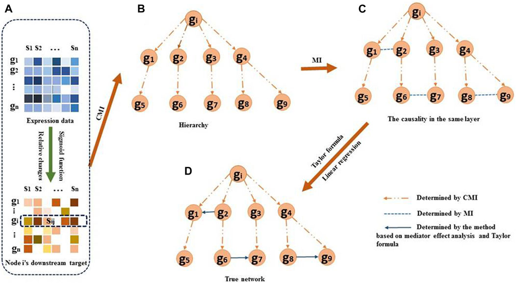
FIGURE 1. Overview of the DDTG method. (A) For each regulator
Causality among hierarchy genes
Some of the downstream targets may be indirectly regulated by gene
The CMI allows measuring the dependency of two genes in the context of a third gene. We assume that
The CMI can be easily calculated using the following equation:
where
Correlations among the genes in the same layer
For the genes in the same layer, the correlations among them are measured by mutual information (MI). MI between two genes
The MI can be easily calculated using the following equivalent formula:
where
Regulatory directions between genes in the same layer
To determine if the regulatory direction in the scenario of
We assume that gene
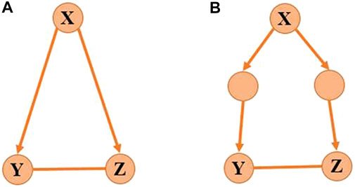
FIGURE 2. Target genes with co-regulator. (A) Genes Y and Z are direct targets of gene X, and (B) genes Y and Z are indirect targets of gene X.
The activity of Y is determined by X and the activity of Z is determined by X and Y. So Y will be the function with respect to X, and Z will be the function with respect to X and Y satisfying Eq. 4 which indicates the causality among X, Y, and Z. The nonlinear regulatory function 4) makes it difficult to computationally identify the model. To address this issue, we apply Taylor expansion which is an accurate substitution of the polynomial function for the nonlinear equation Eq. 4.If
So we need to take the derivative of Z. The first derivative of
The second derivative of
The wild-type data can be viewed as a steady state of GRNs, only for as long as the flow of energy, nutrients, and other molecules is maintained. Hence, while the gene expression level of regulator X is at point
that is,
By substituting (7) into (6), we obtain the second derivative of
that is,
For the value of
By substituting (8) into (11), we obtain the following equation:
Due to
Substituting (10) into the second equation in equation set (13), we obtain the following equation:
The first equation in Eq. 13 is equivalent to the following equation:
that is,
By substituting (16) into (14), we obtain the following equation:
where
On the contrary, we assume that gene Z regulates gene Y, and the gene–gene regulation can be expressed as a nonlinear equation set:
Following the similar process to the aforementioned equation, we estimate parameter
Pseudocode of the DDTG algorithm
To describe the algorithm clearly, the pseudocode of the DDTG algorithm (see Algorithm 1) is provided in detail as follows:
Result
In order to test the predictive power of the DDTG method, DREAM3 datasets (Prill et al., 2010) about Yeast knockout genes with sizes 10, 50, and 100 and two networks of size 10 from the DREAM4 datasets (Daniel et al., 2009) were used. The gold standard networks were generated with the nonlinear ODE systems in which the network structures were determined with detailed dynamics of both transcriptional and translational processes.
The predictive results were evaluated by following measures, that is, sensitivity or true-positive rate (TPR), false-positive rate (FPR), positive predictive value (PPV), accuracy (ACC), and Matthew’s coefficient constant (MCC). Mathematically, they are defined as the following expressions:
where TP, FP, TN, and FN are the numbers of true positives, false positives, true negatives, and false negatives, respectively. TPR and FPR are also used to plot the receiver operating characteristic (ROC) curves, and the area under ROC curve (AUC) is calculated.
To validate the performance of DDTG, we compared it with several popular methods including LP (Wang et al., 2006), RO (Zhang, Liu, Liu, Duval, Richer, Zhao, Hao, and Chen, 2013), regression model-based LASSO (Geert et al., 2012), MI-based ARACNE (Margolin et al., 2006), and random forest-based GENIE3 (Van Anh et al., 2010), where the two alternatives with parameters “sqrt” and “all” in the GENIE3 were considered here, as they performed best in the DREAM challenges. For fair comparison, optimal default values of parameters from previous published articles were used in the running of these comparative algorithms. For example, regularization parameter
Performance on DREAM3 benchmark data
DREAM3 datasets about Yeast knock-out genes with sizes 10, 50, and 100 were used.
First, DDTG was applied to the Yeast gene expression data with network sizes 10 and 10 samples. The comparison of DDTG with other methods is shown in Figure 3A, where DDTG outperforms other methods significantly with an AUC score of 1.000. From Figure 3A, we can see that all of the edges were detected. The performance of DDTG and other methods with respect to PPV, ACC, MCC, and AUC are shown in Table 1, where DDTG is superior to other methods.
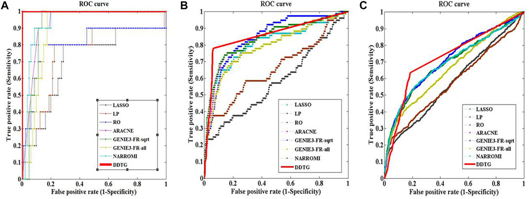
FIGURE 3. ROC curves of several methods on networks with different sizes. The solid line with star points is the ROC curve of method DDTG. (A) The ROC curves on the network with size 10. (B) The ROC curves on the network with size 50. (C) The ROC curves on the network with size 100.
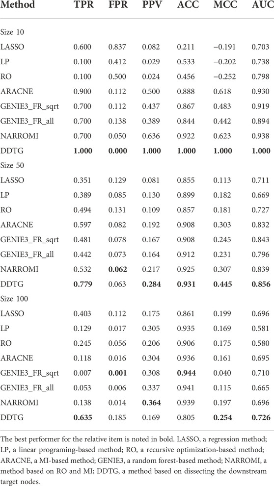
TABLE 1. Comparison on networks with sizes 10, 50, and 100.
Second, DDTG was applied to the Yeast gene expression data with network sizes 50 and 50 samples. The comparison of DDTG with other methods is shown in Figure 3B, where DDTG outperforms other methods significantly with an AUC score of 0.856. From Figure 3B, we can see that most of the edges were recovered. The performance of DDTG and other methods with respect to PPV, ACC, MCC, and AUC are shown in Table 1, where DDTG is superior to other methods.
Third, the Yeast gene expression data with network size 100 and 100 samples were used to evaluate DDTG and other methods. The ROC curves obtained by different methods are shown in Figure 3C, where DDTG outperforms other methods with an AUC score of 0.726. Table 1 shows the results obtained by different methods with respect to distinct performance indices. From the results, we can observe that DDTG performs better than most methods.
Performance on DREAM4 benchmark data
The performance of network inference methods may strongly vary depending on the structural properties of the target networks. In order to assess the performance of DDTG predicting the topology on different target networks, DREAM4 datasets with size 10 were adopted here to evaluate our method.
While DREAM3 benchmarks were of a great value, there were some notable differences between DREAM3 and DREAM4 datasets. First, all the networks in DREAM3 were acyclic, while the networks considered in DREAM4 do contain cycles. Furthermore, a deterministic model was used in the DREAM3, while a stochastic one was used in DREAM4. Finally, both biological noise and experimental noise were added to DREAM4 datasets (Andrea et al., 2010). DREAM4 benchmarks consist of a set of networks with widely varying topologies. Two networks of size 10 from DREAM4 in silico challenge were adopted here to test our method.
Figures 4A,B show the ROC curves by different methods on two different networks of size 10 from DREAM4 challenge. From figures, we can see that the performance of DDTG method is superior to that of other methods with the AUC values of 0.862 and 0.761. Table 2 summarizes the results obtained by different methods with respect to distinct performance indices. From Table 2, we can see that DDTG performs significantly better than other methods. Especially, when the DREAM4 datasets are used to test the performance of these methods, the accuracy of DDTG is still high. However, other methods except DDTG perform better in DREAM3 datasets; their performance decays rapidly in DREAM4 datasets.
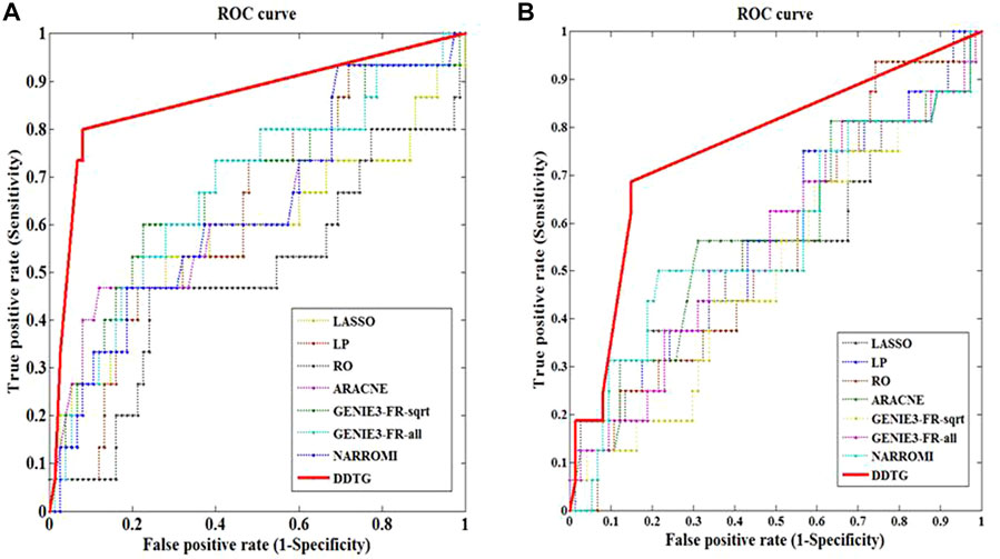
FIGURE 4. ROC curves of several methods on networks with different sizes. The solid line with star points is the ROC curve of method DDTG. (A) The ROC curves on network_1 from DREAM4 datasets with size 10. (B) The ROC curves on network_2 from DREAM4 datasets with size 10.
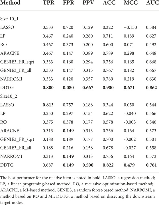
TABLE 2. Comparison on networks from DREAM4 datasets with size 10.
Figure 5 shows the performance of the compared methods on DREAM3 datasets with size 10 and two networks from DREAM4 datasets with size 10. From Figure 5, we can find that the performance of DDTG varies less strongly than that of other methods in different datasets. It indicates that DDTG is more robust than other methods on different networks.
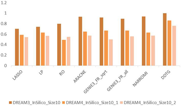
FIGURE 5. AUC comparison of methods on different networks with size 10.
Discussion
In this article, we proposed a novel method DDTG to reconstruct GRNs from gene knockout data. Yet our method can be applied to infer regulatory networks if gene knockdown or over-expression experiments are provided. This algorithm includes two steps. In the first step, the downstream targets are identified by comparing relative change values. In the second step, the hierarchy structure of the downstream targets is determined using CMI and MI. From the results, we can see that clearly DDTG is the best performer on the benchmark datasets. The good performance of DDTG may be contributed by following factors. Genes whose steady state values change after gene knockout can be immediately recognized by comparing the relative change values, which can improve the accuracy of network reconstruction. Meanwhile, due to the sparseness of GRNs, the downstream targets consist of a small number of nodes, which is helpful to reduce the redundant edges. Moreover, we assign a weight to the relative change values using sigmoid function. The parameters of the weight function depend on the expression level of each gene. This can reduce the noise for each gene (higher noise for a higher expression level). Therefore, other methods perform poorly in DREAM4 datasets, but the accuracy of DDTG is still high.
Furthermore, we construct gene–gene regulations using the Taylor formula at the steady-state levels of the wild type, and we use linear regression to determine the causal relationship between genes in the same layer for the first time. Finally, we infer the causal structure of GRNs using CMI and MI. Our method has the advantages of machine learning-based methods, such as making no explicit mechanistic assumptions and more computationally efficient.
Despite the advantages of DDTG, there are also limitations: DDTG is strongly dependent on the accuracy of identifying the downstream target nodes. The spurious downstream target nodes definitely result in spurious edges. For instance, the FPR by DDTG on datasets of size 100 is higher than that of other methods in Table 1. A technique to filter out and remove the impact of the spurious nodes may improve the performance of DDTG and will be considered in DDTG.
Conclusion
We proposed a novel method, namely, DDTG, to improve the accuracy of GRN inference by dissecting the downstream target nodes. In this algorithm, the downstream targets for each gene are identified by comparing the relative change values. Furthermore, the causal structure of downstream targets is determined by CMI and MI. We especially use a weight function to reduce the noise for each regulator and determine the causality between nodes in the same layer using the Taylor formula and linear regression. The method was validated on the benchmark GRNs from DREAM challenge. The results confirmed the effectiveness of our method, which outperformed previous methods.
Data availability statement
The original contributions presented in the study are included in the article/Supplementary Material; further inquiries can be directed to the corresponding author.
Author contributions
ZJ and XZ conceived and designed the experiments. ZJ performed the experiments. ZJ analyzed the data. ZJ and XZ wrote the article. All authors contributed to the article and approved the submitted version.
Funding
This work was supported by the grants from the National Natural Science Foundation of China [32070682], the Technology Innovation Zone Project [1816315XJ00100216], and the CAS Pioneer Hundred Talents Program.
Conflict of interest
The authors declare that the research was conducted in the absence of any commercial or financial relationships that could be construed as a potential conflict of interest.
Publisher’s note
All claims expressed in this article are solely those of the authors and do not necessarily represent those of their affiliated organizations, or those of the publisher, the editors, and the reviewers. Any product that may be evaluated in this article, or claim that may be made by its manufacturer, is not guaranteed or endorsed by the publisher.
References
Aghdam, R., Ganjali, M., Zhang, X., and Eslahchi, C. (2015). CN: A consensus algorithm for inferring gene regulatory networks using the SORDER algorithm and conditional mutual information test. Mol. Biosyst. 11, 942–949. doi:10.1039/c4mb00413b
Ahmed, S. S., Roy, S., and Kalita, J. K. (2018). Assessing the effectiveness of causality inference methods for gene regulatory networks. IEEE/ACM Trans. Comput. Biol. Bioinform. 17, 56–70. doi:10.1109/TCBB.2018.2853728
Algabri, Y. A., Li, L., and Liu, Z-P. (2022). scGENA: A single-cell gene coexpression network analysis framework for clustering cell types and revealing biological mechanisms. Bioengineering 9, 353. doi:10.3390/bioengineering9080353
Altay, G., and Emmert-Streib, F. (2010). Revealing differences in gene network inference algorithms on the network level by ensemble methods. Bioinformatics 26, 1738–1744. doi:10.1093/bioinformatics/btq259
Andrea, P., Nicola, S., and Alberto, D. L. F. (2010). From knock-outs to networks: Establishing direct cause-effect relationships through graph analysis. PloS one 5, e12912. doi:10.1371/journal.pone.0012912
Baruch, B., and Albert-László, B. (2013). Network link prediction by global silencing of indirect correlations. Nat. Biotechnol. 31, 720–725. doi:10.1038/nbt.2601
Butte, A. J., and Kohane, I. S. (2000). Mutual information relevance networks: Functional genomic clustering using pairwise entropy measurements. Pac. Symp. Biocomput. 2000, 418–429. Epub 2000/07/21. doi:10.1142/9789814447331_0040
Chen, G., and Liu, Z. (2022). Inferring causal gene regulatory network via GreyNet: From dynamic grey association to causation. Front. Bioeng. Biotechnol. 10, 954610. doi:10.3389/fbioe.2022.954610
Daniel, M., Prill, R. J., Thomas, S., Claudio, M., Dario, F., and Gustavo, S. (2010). Revealing strengths and weaknesses of methods for gene network inference. Proc. Natl. Acad. Sci. U. S. A. 107, 6286–6291. doi:10.1073/pnas.0913357107
Daniel, M., Thomas, S., Claudio, M., and Dario, F. (2009). Generating realistic in silico gene networks for performance assessment of reverse engineering methods. J. Comput. Biol. 16, 229–239. doi:10.1089/cmb.2008.09TT
Deng, Z., Zhang, J., Li, J., and Zhang, X. (2021). Application of deep learning in plant–microbiota association analysis. Front. Genet. 12, 697090. doi:10.3389/fgene.2021.697090
Finkle, J. D., Wu, J. J., and Bagheri, N. (2018). Windowed Granger causal inference strategy improves discovery of gene regulatory networks. Proc. Natl. Acad. Sci. U. S. A. 115, 2252–2257. doi:10.1073/pnas.1710936115
Gardner, T. S., Di Bernardo, D., Lorenz, D., and Collins, J. J. (2003). Inferring genetic networks and identifying compound mode of action via expression profiling. Science 301, 102–105. doi:10.1126/science.1081900
Geert, G., van Kesteren, R. E., Smit, A. B., and de Gunst, M. C. (2012). Identification of context-specific gene regulatory networks with GEMULA--gene expression modeling using LAsso. Bioinformatics 28, 214–221. doi:10.1093/bioinformatics/btr641
Honkela, A., Girardot, C., Gustafson, E. H., Liu, Y-H., Furlong, E. E., Lawrence, N. D., et al. (2010). Model-based method for transcription factor target identification with limited data. Proc. Natl. Acad. Sci. U. S. A. 107, 7793–7798. doi:10.1073/pnas.0914285107
Hughes, T. R., Marton, M. J., Jones, A. R., Roberts, C. J., Stoughton, R., Armour, C. D., et al. (2000). Functional discovery via a compendium of expression profiles. Cell. 102, 109–126. doi:10.1016/s0092-8674(00)00015-5
Hurley, D., Araki, H., Tamada, Y., Dunmore, B., Sanders, D., Humphreys, S., et al. (2011). Gene network inference and visualization tools for biologists: Application to new human transcriptome datasets. Nucleic Acids Res. 40, 2377–2398. doi:10.1093/nar/gkr902
Jiang, X., and Zhang, X. (2022). Rsnet: Inferring gene regulatory networks by a redundancy silencing and network enhancement technique. BMC Bioinforma. 23, 165–218. doi:10.1186/s12859-022-04696-w
Jiang, Y. J., Aerne, B. L., Smithers, L., Haddon, C., Ish-Horowicz, D., and Lewis, J. (2000). Notch signalling and the synchronization of the somite segmentation clock. Nature 408, 475–479. doi:10.1038/35044091
Karlebach, G., and Shamir, R. (2008). Modelling and analysis of gene regulatory networks. Nat. Rev. Mol. Cell. Biol. 9, 770–780. doi:10.1038/nrm2503
Khatamian, A., Paull, E. O., Califano, A., and Yu, J. (2018). SJARACNe: A scalable software tool for gene network reverse engineering from big data. Bioinformatics 35, 2165–2166. doi:10.1093/bioinformatics/bty907
Kinney, J. B., and Atwal, G. S. (2014). Equitability, mutual information, and the maximal information coefficient. Proc. Natl. Acad. Sci. U. S. A. 111, 3354–3359. doi:10.1073/pnas.1309933111
Krouk, G., Lingeman, J., Colon, A. M., Coruzzi, G., and Shasha, D. (2013). Gene regulatory networks in plants: Learning causality from time and perturbation. Genome Biol. 14, 123. doi:10.1186/gb-2013-14-6-123
Lu, J., Dumitrascu, B., McDowell, I. C., Jo, B., Barrera, A., Hong, L. K., et al. (2021). Causal network inference from gene transcriptional time-series response to glucocorticoids. PLoS Comput. Biol. 17, e1008223. doi:10.1371/journal.pcbi.1008223
Madar, A., Greenfield, A., Ostrer, H., Vanden-Eijnden, E., and Bonneau, R. (2009). The inferelator 2.0: A scalable framework for reconstruction of dynamic regulatory network models. Annu. Int. Conf. IEEE Eng. Med. Biol. Soc. 2009, 5448–5451. doi:10.1109/IEMBS.2009.5334018
Margolin, A. A., Nemenman, I., Basso, K., Wiggins, C., Stolovitzky, G., Favera, R. D., et al. (2006). Aracne: An algorithm for the reconstruction of gene regulatory networks in a mammalian cellular context. BMC Bioinforma. 7, S7. doi:10.1186/1471-2105-7-S1-S7
Modi, S. R., Camacho, D. M., Kohanski, M. A., Walker, G. C., and Collins, J. J. (2011). Functional characterization of bacterial sRNAs using a network biology approach. Proc. Natl. Acad. Sci. U. S. A. 108, 15522–15527. doi:10.1073/pnas.1104318108
Nagoshi, E., Saini, C., Bauer, C., Laroche, T., Naef, F., and Schibler, U. (2004). Circadian gene expression in individual fibroblasts : Cell-autonomous and self-sustained oscillators pass time to daughter cells. Cell. 119, 693–705. doi:10.1016/j.cell.2004.11.015
Prill, R. J., Daniel, M., Julio, S. R., Sorger, P. K., Alexopoulos, L. G., Xiaowei, X., et al. (2010). Towards a rigorous assessment of systems biology models: The DREAM3 challenges. PloS one 5, e9202. doi:10.1371/journal.pone.0009202
Reshef, D. N., Reshef, Y. A., Finucane, H. K., Grossman, S. R., McVean, G., Turnbaugh, P. J., et al. (2011). Detecting novel associations in large data sets. science 334, 1518–1524. doi:10.1126/science.1205438
Riet, D. S., and Kathleen, M. (2010). Advantages and limitations of current network inference methods. Nat. Rev. Microbiol. 8, 717–729. doi:10.1038/nrmicro2419
Rubin, A. J., Parker, K. R., Satpathy, A. T., Qi, Y., Wu, B., Ong, A. J., et al. (2019). Coupled single-cell CRISPR screening and epigenomic profiling reveals causal gene regulatory networks. Cell. 176, 361–376. doi:10.1016/j.cell.2018.11.022
Studham, M. E., Tjärnberg, A., Nordling, T. E., Nelander, S., and Sonnhammer, E. L. (2014). Functional association networks as priors for gene regulatory network inference. Bioinformatics 30, i130–i138. doi:10.1093/bioinformatics/btu285
Tibshirani, R. (2011). Regression shrinkage and selection via the lasso: A retrospective. J. R. Stat. Soc. Ser. B Stat. Methodol. 73, 273–282. doi:10.1111/j.1467-9868.2011.00771.x
Van Anh, H. T., Alexandre, I., Louis, W., and Pierre, G. J. P. O. (2010). Inferring regulatory networks from expression data using tree-based methods. PloS one 5, 4439–4451.
Wang, T., Peng, H., Cao, Y., Xu, J., Xiong, Y., Liu, K., et al. (2022). Dynamic network biomarker analysis reveals the critical phase transition of fruit ripening in grapevine. Genes. 13, 1851. doi:10.3390/genes13101851
Wang, Y., Joshi, T., Zhang, X-S., Xu, D., and Chen, L. (2006). Inferring gene regulatory networks from multiple microarray datasets. Bioinformatics 22, 2413–2420. doi:10.1093/bioinformatics/btl396
Wang, Y., and Liu, Z-P. (2022). Identifying biomarkers for breast cancer by gene regulatory network rewiring. BMC Bioinforma. 22, 308–315. doi:10.1186/s12859-021-04225-1
Yang, B., Bao, W., and Chen, B. (2022). Pgrnig: Novel parallel gene regulatory network identification algorithm based on GPU. Brief. Funct. Genomics 2022, elac028. doi:10.1093/bfgp/elac028
Yang, B., Bao, W., Zhang, W., Wang, H., Song, C., Chen, Y., et al. (2021). Reverse engineering gene regulatory network based on complex-valued ordinary differential equation model. BMC Bioinforma. 22, 448–519. doi:10.1186/s12859-021-04367-2
Zak, D. E., Gonye, G. E., Schwaber, J. S., and Doyle, F. J. (2003). Importance of input perturbations and stochastic gene expression in the reverse engineering of genetic regulatory networks: Insights from an identifiability analysis of an in silico network. Genome Res. 13, 2396–2405. doi:10.1101/gr.1198103
Zhang, A., Xiong, Y., Fang, J., Jiang, X., Wang, T., Liu, K., et al. (2022). Diversity and functional evolution of terpene synthases in rosaceae. Plants 11, 736. doi:10.3390/plants11060736
Zhang, X., Liu, K., Liu, Z. P., Duval, B., Richer, J. M., Zhao, X. M., et al. (2013). Narromi: A noise and redundancy reduction technique improves accuracy of gene regulatory network inference. Bioinformatics 29, 106–113. doi:10.1093/bioinformatics/bts619
Zhang, X., Zhao, J., Hao, J. K., Zhao, X. M., and Chen, L. (2015). Conditional mutual inclusive information enables accurate quantification of associations in gene regulatory networks. Nucleic Acids Res. 43, e31. doi:10.1093/nar/gku1315
Zhang, X., Zhao, X-M., He, K., Lu, L., Cao, Y., Liu, J., et al. (2011). Inferring gene regulatory networks from gene expression data by path consistency algorithm based on conditional mutual information. Bioinformatics 28, 98–104. doi:10.1093/bioinformatics/btr626
Zhang, X-F., Ou-Yang, L., and Yan, H. (2017). Incorporating prior information into differential network analysis using non-paranormal graphical models. Bioinformatics 33, 2436–2445. doi:10.1093/bioinformatics/btx208
Keywords: gene regulatory networks, network inference, downstream targets, causality, machine learning
Citation: Jia Z and Zhang X (2022) Accurate determination of causalities in gene regulatory networks by dissecting downstream target genes. Front. Genet. 13:923339. doi: 10.3389/fgene.2022.923339
Received: 19 April 2022; Accepted: 08 November 2022;
Published: 07 December 2022.
Edited by:
Bin Yang, Zaozhuang University, ChinaReviewed by:
Tao He, San Francisco State University, United StatesZhi-Ping Liu, Shandong University, China
Copyright © 2022 Jia and Zhang. This is an open-access article distributed under the terms of the Creative Commons Attribution License (CC BY). The use, distribution or reproduction in other forums is permitted, provided the original author(s) and the copyright owner(s) are credited and that the original publication in this journal is cited, in accordance with accepted academic practice. No use, distribution or reproduction is permitted which does not comply with these terms.
*Correspondence: Xiujun Zhang, emhhbmd4akB3YmdjYXMuY24=