 Mélanie Raymond
 Marie-Hélène Descary†
 Fabrice Larribe
- Department of Mathematics, Université du Québec à Montréal, Montréal, QC, Canada
Introduction: Over the years, many approaches have been proposed to build ancestral recombination graphs (ARGs), graphs used to represent the genetic relationship between individuals. Among these methods, many rely on the assumption that the most likely graph is among those with the fewest recombination events. In this paper, we propose a new approach to build maximum parsimony ARGs: Reinforcement Learning (RL).
Methods: We exploit the similarities between finding the shortest path between a set of genetic sequences and their most recent common ancestor and finding the shortest path between the entrance and exit of a maze, a classic RL problem. In the maze problem, the learner, called the agent, must learn the directions to take in order to escape as quickly as possible, whereas in our problem, the agent must learn the actions to take between coalescence, mutation, and recombination in order to reach the most recent common ancestor as quickly as possible.
Results: Our results show that RL can be used to build ARGs with as few recombination events as those built with a heuristic algorithm optimized to build minimal ARGs, and sometimes even fewer. Moreover, our method allows to build a distribution of ARGs with few recombination events for a given sample, and can also generalize learning to new samples not used during the learning process.
Discussion: RL is a promising and innovative approach to build ARGs. By learning to construct ARGs just from the data, our method differs from conventional methods that rely on heuristic rules or complex theoretical models.
1 Introduction
The ancestral recombination graph (ARG) (Griffiths, 1991; Griffiths and Marjoram, 1996; 1997) is used to represent the genetic relationship between a sample of individuals. It plays a key role in biology analysis and genetic studies. For example, it can be used to estimate some parameters of a population or for genetic mapping (Stern et al., 2019; Fan et al., 2023; Hejase et al., 2022; Link et al., 2023; Larribe et al., 2002). It is described as “the holy grail of statistical population genetics” in Hubisz and Siepel (2020). Unfortunately, since we cannot go back in time, it is impossible to know the real relationship between a set of genetic sequences. Consequently, we have to infer it, and even today, this is still a difficult task.
Over the years, many approaches have been proposed to build ARGs (Lewanski et al., 2024). Some of these approaches are based on the coalescent model (Rasmussen et al., 2014; Heine et al., 2018; Hubisz et al., 2020; Mahmoudi et al., 2022), but they are computationally intensive. To overcome this problem, other methods have been developed (Speidel et al., 2019; Kelleher et al., 2019; Zhang et al., 2023; Wohns et al., 2022), but most approaches face a trade-off between accuracy and scalability (YC Brandt et al., 2022).
Heuristic algorithms have also been proposed. These methods rely on the assumption that the fewer recombination events, the more likely the graph. KwARG (Ignatieva et al., 2021), SARGE (Schaefer et al., 2021), RENT+ (Mirzaei and Wu, 2017), ARG4WG (Nguyen et al., 2016), and Margarita (Minichiello and Durbin, 2006) are some examples of these heuristic algorithms. These methods do not learn from data, but are based on strict rules established by the knowledge of genetic experts. Moreover, they aim to build the maximum parsimony graph, but parsimonious does not necessarily mean better. In fact, the results in Nguyen et al. (2016) show that ARG4WG builds ARGs with fewer recombination events than Margarita, but when they compare the ARGs built with both algorithms to the real genealogy (using simulated data), Margarita gets slightly better results. Our approach is strictly data-driven and does not rely on prior knowledge of genetics. It also allows to obtain a distribution of ARGs of different lengths, which is a great advantage over these heuristic algorithms.
In this manuscript, we propose a novel approach to build ARGs using Reinforcement Learning (RL) (Sutton and Barto, 2018). With recent advances in artificial intelligence, RL has been developed for applications in multiple fields, from games to transportation to marketing services. Machine learning (ML) and RL have also been used for various applications in biology and in genetics (Mahmud et al., 2018). For example, ML has been used to infer demographic history, to detect natural selection, and to estimate recombination hotspots, to name a few (Sheehan and Song, 2016; Flagel et al., 2019; Smith et al., 2017; Torada et al., 2019; Sanchez et al., 2021; Gower et al., 2021; Chan et al., 2018). On the other hand, Chuang et al. (2010) used RL for operon prediction in bacterial genomes, Bocicor et al. (2011) used it to solve the DNA fragment assembly problem, and Zhu et al. (2015) used it to establish a protein interaction network. However, to our knowledge, RL has not been used to build ARGs.
If we assume that the most likely graph is one with few number of recombination events, this means that it is among the shortest ones. Throughout this paper, we consider the number of events in an ARG as its length. Therefore, the shortest ARG is equivalent to the maximum parsimony ARG or the one with the fewest number of recombination events. Searching for the shortest ARG means that we are looking for the shortest path between a set of genetic sequences and their most recent common ancestor (MRCA). We seek to leverage the similarities between building the shortest path between a set of genetic sequences and their MRCA and the shortest path to the exit in a maze, a classic RL problem.
A famous example of RL is the computer program TD-Gammon (Tesauro, 1991; 1994; Tesauro et al., 1995; Tesauro, 2002), which learned to play backgammon at a level close to that of the greatest players in the world. But even more than that, TD-Gammon influenced the way people play backgammon (Tesauro et al., 1995). In some cases, it came up with new strategies that actually led top players to rethink their positional strategies. So we wanted to use RL to see if a machine could learn the rules established by humans for building short genealogies like those used in heuristic algorithms, or even better, discover new ones.
In the short term, our aim was not to develop a method that could be immediately applied on real data, or that could compete with existing methods. Rather, as a first step, we wanted to explore the possibility of using RL to build short ARGs. The essence of this work was to explore whether it is possible to build maximum parsimony ARGs with a method that is based solely on data and does not rely on knowledge of genetics. In a second phase, we will be interested in improving and refining our method so that it can be used with large-scale data.
The main contributions within this manuscript are:
• A new approach using RL to build a distribution of ARGs for a given set of sequences used during training. This is detailed in Sections 2.3.2, 3.2.
• A new method based on RL to build a distribution of ARGs for a set of
• The development of an ensemble method to improve the generalization performance, which we discuss in Sections 2.3.3, 3.3.
Section 2.1 introduces genetic concepts necessary for a good understanding of the work. In Section 2.2, we present in detail different methods used to solve RL problems and, in Section 2.3, we explain how we apply them to build ARGs. Our experiments and the results obtained are presented in Section 3. Finally, Section 4 concludes the paper with a discussion of possible improvements and future work.
2 Materials and methods
2.1 Background in genetics
First, in this section, we look at some genetic concepts to get a better understanding of what an ARG represents and how it is built.
The ARG is used to represent the transmission of genetic material from ancestors to descendants. To account for species diploidy, each individual is represented by 2 sequences in the ARG. In this paper, a genetic sequence represents a sequence of single nucleotide polymorphisms (SNPs). The transmission of genetic material occurs through three types of events: coalescence, mutation, and recombination, which are described in the following subsections. The goal of our reinforcement learning process will be to learn which actions to take between these three in order to build ARGs among the shortest ones (those with the fewest recombination events).
2.1.1 Coalescence
Coalescence occurs when two sequences have a common ancestor. On Figure 1, coalescences are represented by events 4, 5, 7, and 9. The coalescence process is a continuous-time stochastic process introduced by Kingman (1982). For a given sample, the states of the process are all possible genetic sequence subsets. In fact, a state corresponds to the sequences present in a generation of a genealogy. To go from one state to another, two sequences must coalesce. When building ARGs from the present to the past, the coalescence event is represented by two sequences merging, and thus reducing the sample size by 1.
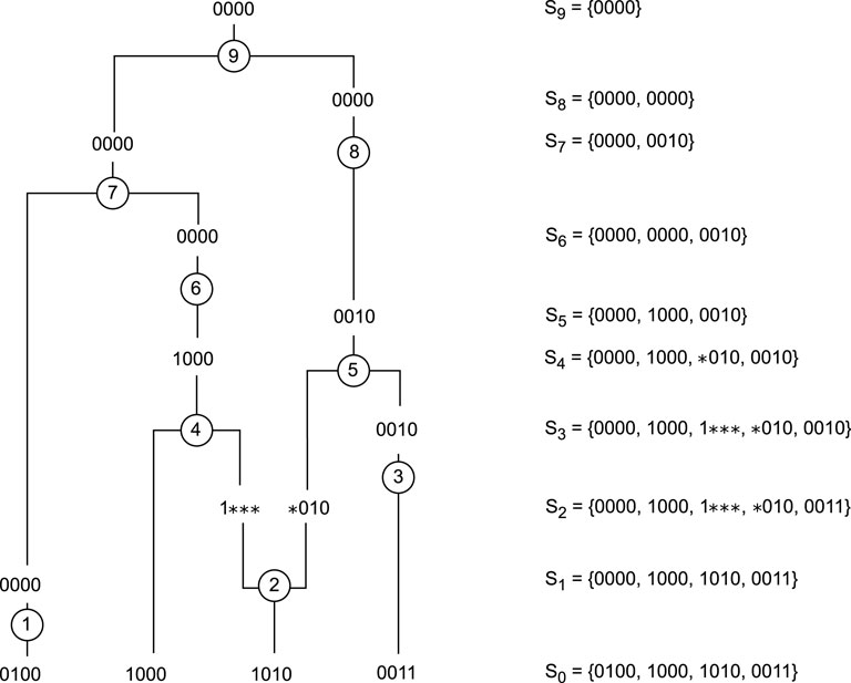
Figure 1. Example of an ARG with 4 sequences of 4 SNPs. Events 1, 3, 6, and 8 are mutations, events 4, 5, 7, and 9 are coalescences, and event 2 is a recombination. The right column represents the state of the system between events.
2.1.2 Mutation
There are several types of mutations, but in this paper, we will focus on those that occur when the allele of a marker is altered. Mutations are represented by events 1, 3, 6, and 8 on Figure 1. There are several models for inserting a mutation into the coalescence process. The infinite sites model is a commonly used model. In this model, only one mutation event is allowed per marker position, resulting in non-recurrent mutations. We represent the allele derived from the MRCA as “0”, and the mutated allele as “1”. Therefore, each sequence in our ARG is represented by a vector of 0s and 1s. Using this model means that in the learning process, it will only be possible to select a mutation event if a mutated allele is present on a single sequence.
2.1.3 Recombination
Recombination occurs when genetic material is shuffled, and a child inherits a mixture of the two homologous chromosomes from one of its parents. The second event on Figure 1 is a recombination. When building ARGs, a recombination event introduces non-ancestral material, genetic material that was not present in the original sample, as shown in Figure 1. In this paper, it is represented by “
Going back in time, recombination events increase the sample size by 1, which may somehow seem to take us away from our goal of ending with a single sequence. However, they are sometimes the only possible events and are therefore necessary. Learning the right recombination events, the ones that lead to the shortest ARGs, represents the main challenge of our learning process.
2.1.4 Heuristic algorithms to build ARGs
Among the different methods used to build ARGs, heuristic algorithms are the closest to what we propose, in the sense that they are optimized to build the shortest graphs. ARG4WG (Nguyen et al., 2016) is one of these algorithms and manages to build short ARGs. It builds ARGs starting from the present and going back in time; starting with coalescence, then doing mutation. If neither coalescence nor mutation is possible, it seeks the pair of sequences with the longest shared end, and performs a recombination event on one of the sequences. The sequence resulting from the recombination that contains the shared segment is then coalesced with the other sequence in the pair.
We will compare the length of the ARGs built with RL to those built with ARG4WG to evaluate the performance of our method.
2.2 Background in reinforcement learning
In this section, we introduce the key concepts of reinforcement learning based on Sutton and Barto (2018).
In reinforcement learning, the learner, also called the agent, learns the action to take in order to maximize a reward given the current situation. In many cases, the problem can be represented as a Markov decision process (MDP) where
representing the probability of going to state
As mentioned in the introduction, with RL, an agent can learn to get out of a maze as quickly as possible (Sutton and Barto, 2018). In this last problem, the set of states is the set of all possible locations in the maze, and the actions are the directions the agent can take, for example, up, down, right, and left. Typically, in this type of problem, the agent receives a reward of
In many RL problems, the interactions between the agent and its environment can be broken into subsequences, which we call episodes. For example, games fall into this category where the agent learns by playing multiple games. Each time a game ends, the agent starts a new one to improve its performance. The end of each game represents the end of a learning episode. In the maze problem, an episode begins when the agent enters the maze and ends when it escapes.
In RL, a policy
Similarly, we have:
These equations are called the Bellman equations. Under optimal policy, they are called Bellman optimality equations and are written as follows:
and
Returning to the maze problem, to learn the shortest escape path, the agent must go through the maze many times. At the beginning of each episode, he is placed in one of the maze’s location, and each time he successfully escapes represents the end of an episode. At each time step
2.2.1 Tabular methods
Solving a RL problem boils down to solving the Bellman optimality equations. If the state space
In a perfect world, we can solve our problem by listing all the states and actions in a table and by using dynamic programming to solve the Bellman equations. The idea is to start with a random policy
Algorithm 1.Value Iteration, output:
1:
2:
3: Initialize
4: repeat
5:
6: for each
7:
8:
9:
10: end for
11: until
12: for each
13:
14: end for
15: Return
In the end, in the optimal policy, all actions
Unfortunately, since we do not live in a perfect world, in practice, these methods are not really applicable to problems with a large set of states, such as backgammon, where there are more than
2.2.2 Approximation methods
Approximation methods in RL can be seen as a combination of RL and supervised learning. Instead of estimating the value of each state by visiting all of them, we are looking for a function that approximates the value of the states such that the value of a state never visited can be approximated based on the value of similar states already encountered. In other words, we are looking for
where
where
In RL, we do not know
From a linear function to a multi-layer artificial neural network (NN) (Montesinos Lo´pez et al., 2022),
For example, in our maze problem, assuming the maze can be represented as a 2D grid, then the feature vector could be
2.3 Proposed methodology
In this section, we propose a new way to build ARGs inspired by the maze problem and the RL methods presented in the previous section.
We assume that the most likely graph is among those with the fewest recombination events, so we are looking for the shortest path between a set of genetic sequences (maze entry) and their MRCA (maze exit). The initial state is a sample of genetic sequences. The graphs are built starting from the present and going back in time. Therefore, the other states of our system are our sample at different moments in the past. The final state is the MRCA, which is represented by a single sequence containing only 0s. For example, in Figure 1, the initial state is
A coalescence between two sequences is possible if all their ancestral material is identical. If the action chosen by the agent is a coalescence between two identical sequences of type
If the coalescence is between two sequences of different types
For the mutations, we assume the infinite sites model, so a mutation is only possible if the mutated allele is present on a single sequence. If the agent chooses a mutation on the
Finally, a recombination is possible on any sequence that has at least two ancestral markers, with the exception of the sequence containing only 0s, because this sequence represents the MRCA and it would not be useful to recombine it, it would even be counterproductive and would lead to strictly longer ARGs. The agent will have to choose which sequence to recombine and the recombination point, which can be between any two ancestral markers. The recombination will result in a new state where the sequence of type
Let’s consider the initial state in Figure 1,
• a mutation on the second marker of the sequence 0100, and one on the fourth marker of the sequence 0011 (under the infinite sites model, mutations on the first and third markers are not possible because they are on two sequences),
• 12 recombinations: for all sequences, a recombination between the first and second markers, one between the second and third markers and one between the third and fourth markers.
There is no coalescence possible because no sequences have identical ancestral material.
The episode ends when the agent reaches the MRCA. The agent will learn to construct short ARGs by running several episodes, i.e., by building several genealogies. The first ones will be very long, but eventually, the agent will find the optimal path to reach the MRCA. Remember that the cumulative sum of rewards is equal to minus the number of actions, so by aiming to maximize its rewards, the agent will eventually find short paths.
2.3.1 Tabular methods: a toy example
The first way to learn to construct short ARGs is to use the tabular methods described in Section 2.2.1. When building ARGs, we know the dynamics of the environment because an action can only lead to one state and because we give a reward of
We use this equation in the value iteration algorithm (Algorithm 1) and can find an optimal policy for a given set of genetic sequences.
Once the optimal policy is determined, we can build a variety of ARGs for a given sample. And since the policy maps each state to a distribution over actions, we can compute the probability of each ARG, which gives us a distribution of genealogies. This can be interesting in genetic mapping, for example, and is a great advantage of RL over heuristic algorithms that consider all ARGs as likely.
The problem is that the dimension of the state space grows extremely fast as the sample size increases (number of SNPs or number of sequences). In fact, Song et al. (2006) have shown that, for a sample of
2.3.2 Approximation methods
As presented in Section 2.2.2, we are now looking for a function
For building ARGs, we have to find a feature vector whose dimension is independent of the number of sequences in a state
To further reduce the dimension of
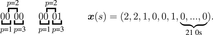
Figure 2. Example of the feature vector for the state with the sequences 0000 and 0001, using blocks of 2 markers with an overlap of one step shift. There are 9 possible blocks of 2 markers and 3 different possible positions. The multiplicity of the first block at position 1 is 2, at position 2 is 2, and at position 3 is 1. The multiplicity of the second block at position 1 is 0, at position 2 is 0, and at position 3 is 1. The multiplicity of all other blocks is 0 for the 3 possible positions.
For example, let’s consider sequences of 4 markers and use blocks of 2 markers with an overlap of one step shift. We have
For example, let’s consider the state
The idea of using blocks of markers came from the four-gametes test (Hudson and Kaplan, 1985). To determine if recombination is necessary to build the ARG of a given set of sequences, we look at blocks of two markers. Under the infinite sites model, since only one mutation event is allowed per marker position, then a recombination is required if blocks 01, 10, and 11 appear at the same site. We tried different block sizes, with and without overlap, and the best results were obtained with blocks of three markers overlapping by one step shift.
Representation by blocks of markers was the best solution we found to reduce the dimension of the feature vector, but it is still computationally intensive. Our method currently only works with sequences of
We start the learning process with a sample of genetic sequences. We keep only one sequence of each type and use this sample as our initial state. After each episode, corresponding to the construction of a genealogy, we update the parameter vector
After generating a certain number of episodes, we use the estimated value function
Even though the agent only learned with a reduced sample (a sequence of each type instead of the entire sample), the policy can be applied to the entire sample, as shown by the results in Section 3.2. It is therefore interesting to note that the agent can learn to build ARGs of a large sample of sequences by keeping only the set of unique sequences from that sample. In other words, if we consider the sample containing 10 sequences 0100, 9 sequences 1000, 3 sequences 1010 and 4 sequences 0011, the agent can learn to build ARGs for this sample by training with a sample containing only 4 sequences: 0100, 1000, 1010 and 0011.
Algorithm 2.Gradient Monte Carlo Algorithm.
1: Input: a differentiable function
2: Algorithm parameters: step size
3: Initialize value-function parameters
4: loop (for each episode):
5: Generate an episode
6: for each step of the episode,
7:
8: end for
9: end loop
10: Return
Applying the optimal policy usually results in the construction of similar ARGs. However, to obtain a greater variety of genealogies, it is possible to adjust the final policy. Instead of following the optimal policy, it is possible to assign a probability to each action or to the
Even though learning how to construct a graph from a specific sample has its uses, this method learns to build genealogies only for a specific sample and the learning process has to be repeated for each new sample. Consequently, the next section describes the process we designed to generalize learning so that the agent learns to build genealogies for any sample with sequences of
2.3.3 Generalization using ensemble methods
Generalization in RL (Korkmaz, 2024) is not an easy task. Zhang et al. (2018) have shown that agents with optimal performance during training can have very poor results in environments not seen during training. One way they alleviated this issue in a maze problem was to spawn the agent at a random initial location. The maze was exactly the same, but the agent always started an episode in a new location. They used this approach as a regularizer during training. Brunner et al. (2018) used a similar approach by changing the initial state, but instead of changing the initial location, they changed the entire maze configuration. At the beginning of each episode, the agent was placed in a maze that was randomly selected from a training set of different mazes.
To generalize learning when building ARGs, our idea was to allow the agent to learn by training with different samples. We take one large set of sequences, a population, and divide it into three smaller sets: a training set, a validation set, and a test set. An episode begins with a sample of sequences and ends when the agent reaches the MRCA. At the start of each episode, the initial state is determined by randomly drawing a fixed number of
Zhang et al. (2018) have shown that agents with similar training performance can have very different performance in environments not seen during training. Therefore, the validation set is divided into
Although the agent eventually succeeds in building graphs for the majority of the
Although the goal is to build short ARGs, we feel it is more important that the model generalize well, even if that means building slightly longer genealogies. Therefore, we consider the best model to be the one with the smallest proportion of infinite-length genealogies. If more than one model has the same proportion, the one with the smallest average minimum length is considered the best.
The test set is then used to evaluate and compare the best models obtained with different values of
However, even with the best models, we still have a problem of infinite-length ARGs. Therefore, to tackle the problem of infinite-length ARGs and to stabilize learning, we use ensemble methods.
Ensemble methods, such as boosting (Freund and Schapire, 1995) and bagging (Breiman, 1996), are often used in supervised learning to address two issues: the stability and the computational complexity of learning (Shalev-Shwartz and Ben-David, 2014). The idea behind boosting is to aggregate weak learners, which we can think of as a model that is slightly better than a random guess, in order to get an efficient learner.
Boosting is also used in RL (Brukhim et al., 2022; Wang and Jin, 2018). For example, Wang and Jin (2018) proposed a Boosting-based deep neural networks. Their approach combines the outputs of
We draw on these different approaches for our problem. We train
In random forests, a well-known example of ensemble methods, Breiman (2001) has shown that two elements have an impact on the generalization error: the strength of each individual tree in the forest and the correlation between them. High strength and low correlation lead to lower generalization error. In particular, random forests can produce low generalization error even with weak individual learners as long as their correlation is low. Therefore, to improve the accuracy of our model based on ensemble methods, we aim to obtain strong individual agents, but more importantly, agents with low correlation between them.
To estimate the value function, we use the same architecture and the same RL algorithm for each agent, but we have changed the initialization of the parameter vector. We stop the training after using the same number of episodes for each agent and compare the stored models with the validation set. For each agent, we select the model that performs best on the validation set (smallest proportion of infinite genealogies). We then use three different approaches. First, we take the average of the outputs of the
We use the test set to compare the performance of the three approaches. The results are presented in Section 3.3.
3 Results
3.1 Tabular methods
We used tabular methods on two samples of 4 sequences of 4 markers. The first sample contained the sequences 0011, 1011, 1000, 1100, while the second sample contained the sequences 0101, 1000, 1010 and 1101. The optimal policy obtained after following the Algorithm 1 allowed us to construct 758 genealogies of length 9 for the first sample and 414 ARGs of length 9 for the second. Using tabular methods and dynamic programming, we actually find all the possible shortest ARGs. We consider the number of actions taken in a genealogy as its length. For example, the length of the ARG in Figure 3 is 9. Using ARG4WG also produced ARGs of length 9, but resulted in the construction of only 8 different genealogies for each sample. This shows that RL allows us to learn a much larger variety of possible ARGs as well as a distribution over them, an interesting advantage of RL over heuristic algorithms.
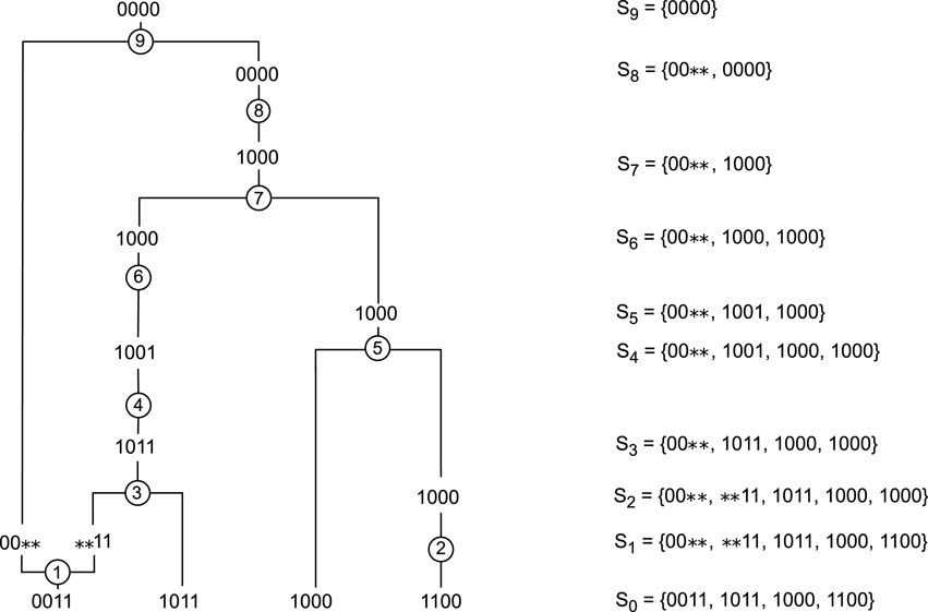
Figure 3. Example of an ARG built starting with
Figure 3 shows an ARG built after following the optimal policy for the first sample,
Although tabular methods cannot be used on large samples, it is still interesting to note that they find different rules than the heuristic algorithms, which makes it possible to generate a wide variety of ARGs.
3.2 Approximation methods: same initial state
For the approximation methods, we simulate 60 different samples on a region of 25 kb long with the Hudson model using msprime (Baumdicker et al., 2022), a widely used package for simulating data sets based on the coalescent process. For all samples, we set the population size to 10,000, and use a mutation rate of
We used
Figure 4 shows the moving average of the lengths over 100 episodes for 20 of the 60 samples used. The results for the 60 samples are available in the Supplementary Material. In many scenarios, the length of the ARGs built during training seems to stabilize after just over 1,000 genealogies. Using the optimal policy obtained after 10,000 episodes, we built ARGs for each of the 60 samples. We compared the length of these genealogies to those obtained using ARG4WG. As shown in Table 1, our method builds ARGs of similar length to those built with ARG4WG. For 48 samples, the ARGs built with RL have the same length as those built with ARG4WG, for 6 samples, the length is shorter with RL, and for 6 samples, the length is shorter with ARG4WG.
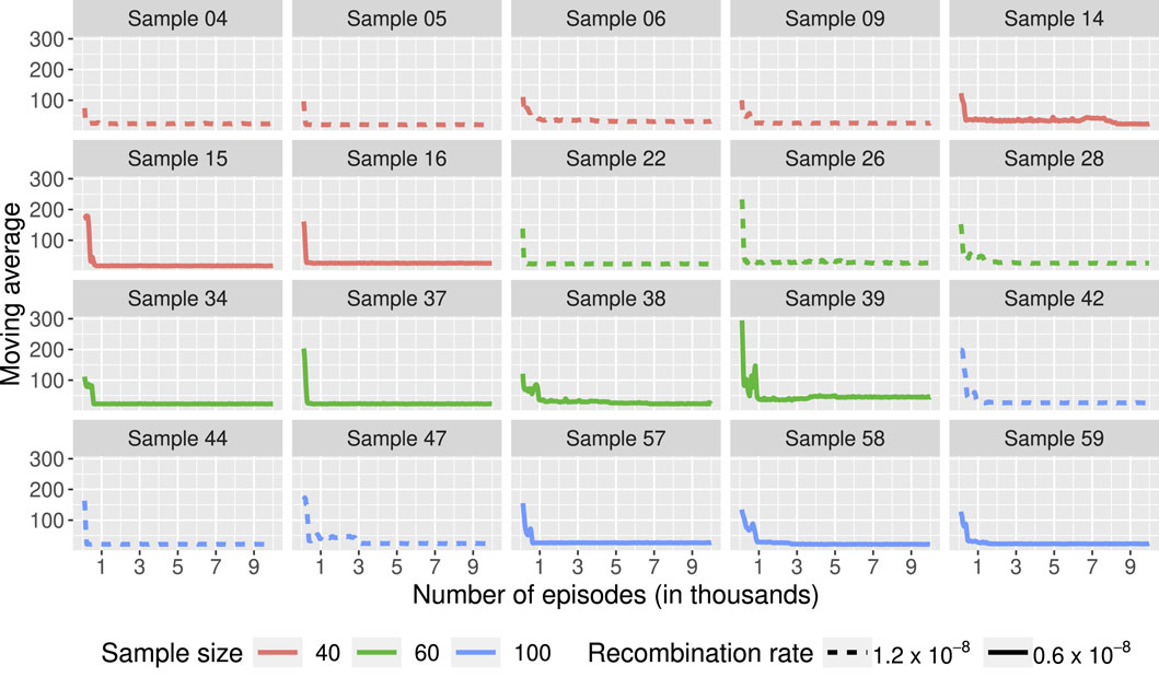
Figure 4. Moving average of the lengths of the ARGs built during training over 100 episodes. Each box represents a learning process using the same sample as initial state. 60 samples were used with different sample sizes (40, 60, 100) and different recombination rates (
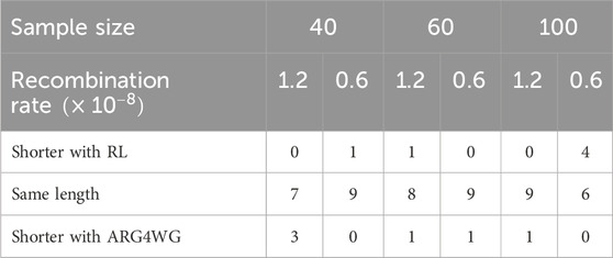
Table 1. Comparison between ARGs built with RL and those built with ARG4WG on 60 different samples. The table shows the number of ARGs shorter with RL, the number of ARGs of the same length, and the number of ARGs shorter with ARG4WG according to the sample size and the recombination rate used to generate the sample.
These results are really interesting: it means that the agent, without any pre-programmed rules, can learn to build ARGs that are as short as those built with a heuristic algorithm optimized to build short ARGs. Even better, in some cases the agent learns new rules that lead to shorter ARGs. The agent can also adjust its optimal policy to get a wider variety of ARGs, another great benefit.
3.3 Generalization and ensemble methods
Now, to generalize our learning, we used msprime to simulate a sample of 15,500 sequences on a region of 10 kb long with the Hudson model. We set the population size to 1,000,000. We used a recombination rate of
We used
We used the validation set to compare models obtained at different times during training. Even though the length of the genealogies seems to stabilize during training, the performance of the models on the validation set is quite variable. We divided the validation set into
We used the test set, divided into
In particular, when we look at the results on different test samples in Figure 5, we can see that one model may be better than another for one sample, but may be worse for another sample. Figure 5 shows the length of the ARGs built by 13 different agents trained with
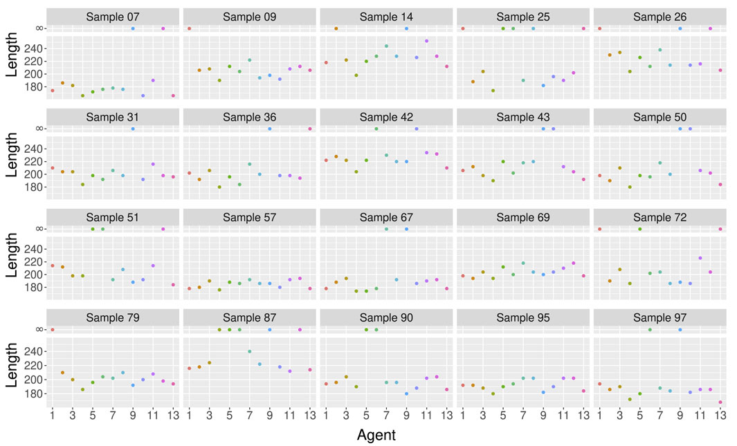
Figure 5. Length of the ARGs built by 13 different agents trained with
To use ensemble methods, we trained
We divided the validation set into
1. Mean: We take the mean of the outputs of the 13 models to estimate the value function. We choose the action
2. Majority: We look at the actions chosen by the 13 models obtained and choose the most frequent one.
3. Minimum: We build an ARG with each of the 13 models and keep the shortest one.
The results obtained are shown in Figure 6. The last method is definitely the best. It builds the shortest genealogy on
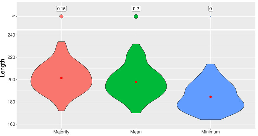
Figure 6. Distribution of lengths of ARGs built from 100 test samples of 50 sequences of 10 SNPs according to three different ensemble methods: majority, mean, and minimum. ARGs of length 400 are considered as infinite-length genealogies. The red dot represents the average length.
Figure 7 shows the proportion of infinite-length genealogies and the average length of the ARGs built on the test set with the third method as a function of the number of models used in the ensemble. As we can see, we eliminate the infinite-length genealogies with only 3 agents in the ensemble. For the average length, we see a great improvement with 4 or 5 agents in the ensemble and the length stabilizes with 11 models. Therefore, our suggestion is to train 12 to 15 independent agents to obtain an efficient ensemble model.
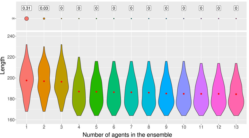
Figure 7. Distribution of lengths of ARGs built from 100 test samples of 50 sequences of 10 SNPs using the third ensemble method (minimum) according to the number of agents used in the ensemble. ARGs of length 400 are considered as infinite-length genealogies. The red dot represents the average length.
The agents were added to the ensemble as they were trained, but we have tried different orders to add them to the ensemble and usually see an improvement in the average length with 5 agents and a stabilization around 10 agents. To eliminate infinite-length genealogies, 2 or 3 agents are usually sufficient. Of the 50 orders we tried, the most agents needed to eliminate infinite-length ARGs was 6. The results are presented in the Supplementary Material.
We compared the results obtained on the test set with the third ensemble method to those obtained with ARG4WG. On average, ARG4WG builds shorter genealogies than our RL method, but the difference is not huge, as shown in Figure 8. For some samples, our method even builds shorter ARGs than ARG4WG.
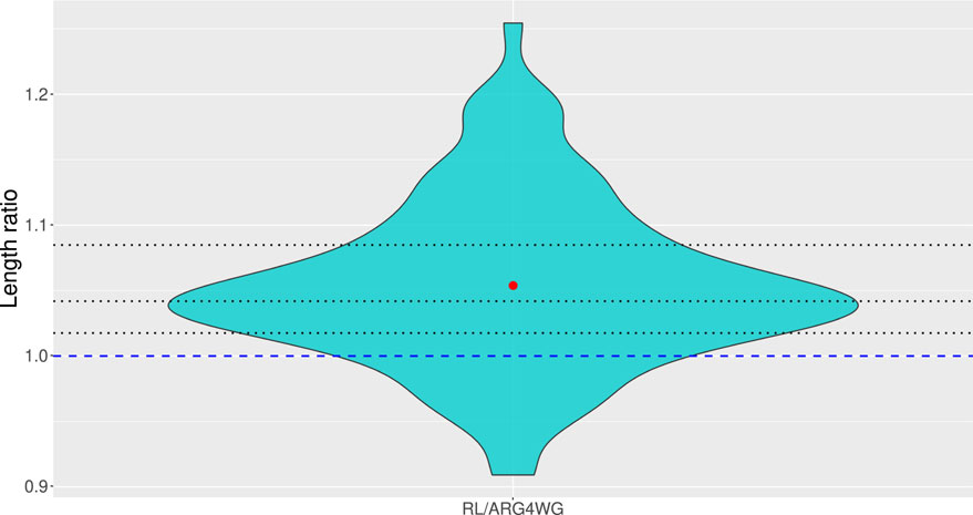
Figure 8. Distribution of ratios between the length of the ARGs built with our third ensemble method (minimum) and those built with ARG4WG from 100 test samples of 50 sequences of 10 SNPs. The dashed blue line represents a ratio of 1, meaning that all ARGs above the line were longer with our method and all ARGs below the line were shorter with our method than with ARG4WG. The dotted black lines represent the quartiles.
It is really interesting to see that our method builds ARGs for any new sample, even samples much larger than those used during training, with lengths around 90%–120% of the lengths of the ARGs built with ARG4WG, an algorithm optimized for building short ARGs. Our method also allows to build a wide variety of short ARGs by adjusting the optimal policy and/or by keeping the ARGs built by different agents, which is a great advantage.
4 Discussion
Our goal with this work was not to compete with existing methods, but rather to explore the potential of a new approach based on machine learning techniques. We wanted to explore how well an RL agent could learn to build short ARGs, without any prior knowledge of genetics, and the first results are very promising. Our results show that RL can be used to obtain a distribution of short ARGs for a given set of genetic sequences, by adapting the optimal policy. The best way to do this is to use this set of sequences as the initial state and to use the same initial state throughout the learning process. However, this means repeating the learning process for each new sample, which is not ideal. To avoid this problem, we have shown that it is possible to learn to build a distribution of short genealogies for different samples from the same population by changing the initial state at the beginning of each episode and by using ensemble methods.
Our results have shown that good performance on the training set does not necessarily translate into good performance on samples not seen during training. Therefore, we recommend using a validation set to determine which models to use as final models. The validation set can also be used to determine when to stop learning, but this remains a question to be discussed. Our results have shown that we can have a good model on the validation set after a certain number of episodes, but we can have a better one after a few more. So for now, we think the best approach is to run more episodes than necessary and select as the final model the one with the best performance on the validation set. Eventually, it would be interesting to establish criteria for determining when to stop learning.
Our results also show that learning can be generalized to larger sample sizes. Thus, it is not necessary to learn with samples of
To evaluate the performance of our method, we compared the length of the ARGs built with RL to those built with a state-of-the-art method used to build short ARGs. Assuming that the most likely graph is among the shortest ones is a strong assumption. In this context, we believe that in future work, it would be really interesting to study the closeness between short ARGs and the true ARGs. In particular, it would be interesting to assess whether our method, being based on data, can build graphs that are close to the real ARGs. As we are currently using samples with sequences of only 10 SNPs, we do not believe that comparing the reconstructed ARGs with the true topology of the ARG would lead to meaningful or relevant results at the moment.
As this work was primarily intended to be exploratory, several improvements are possible and deserve to be explored in future work. The essence of this work was to see if an RL agent could learn rules for building short ARGs on its own, without any prior knowledge of genetics. But we have to face the fact that in order to improve its performance, we might have to introduce some genetic knowledge into the model. This is not surprising, since a similar approach was taken with TD-Gammon. Its first version, TD-Gammon 0.0, was developed with almost no backgammon knowledge, but to improve its performance, hand-crafted backgammon features were incorporated in the second version, TD-Gammon 1.0 (Tesauro, 1994). In our problem, one thing we could do is use a restricted action space (Farquhar et al., 2020) and prohibit some actions. For example, we could forbid the coalescence of two sequences resulting from a recombination. It could also help solve the problem of infinite-length genealogies.
To incorporate genetic knowledge into the model, we could also modify the feature vector
Another possible improvement is to look at more than one action at a time. For example, TD-Gammon 2.0 and 2.1 (Tesauro et al., 1995) improved by performing 2-ply searches, where a ply corresponds to a move made by a player. So instead of just selecting the move that leads to highest value state, the program would also consider the opponent’s possible dice rolls and moves to estimate the value of the states. Versions 3.0 and 3.1 of TD-Gammon (Tesauro, 2002) even perform 3-ply searches. This idea could be really interesting for building ARGs, and could help avoid infinite-length genealogies by preventing recombination followed by coalescence of the resulting sequences.
Using a different RL algorithm is another thing we could try. Instead of waiting until the end of an episode to update the parameter vector
Finally, the main limitation of our method is the number of SNPs used. Since we seem to be able to generalize learning on sample of
In conclusion, our research shows that RL is a promising method to address an important challenge in genetics: building accurate and efficient ARGs. It is a new and innovative approach that allows obtaining a distribution of short ARGs for a specific sample, as well as for new samples not used during the learning process, which can be of interest in genetic mapping, for example,. Our data-driven methodology differs from conventional methods that rely on heuristic rules or complex theoretical models built on strong hypotheses. By learning to build ARGs only from the data, our method has the potential to produce more realistic results and may lead to new rules for building short ARGs.
Data availability statement
The datasets presented in this study can be found in online repositories. The names of the repository/repositories and accession number(s) can be found below: https://github.com/MelaRay/ARGs_through_RL.
Author contributions
MR: Conceptualization, Formal Analysis, Funding acquisition, Methodology, Software, Visualization, Writing – original draft. MD: Conceptualization, Supervision, Writing – review and editing. CB: Conceptualization, Supervision, Writing – review and editing. FL: Conceptualization, Supervision, Writing – review and editing.
Funding
The author(s) declare that financial support was received for the research and/or publication of this article. This work was supported by the Fonds de recherche du Québec–Nature et technologie (#317396 to MR), and the Natural Sciences and Engineering Research Council of Canada (CGS M to MR). The funders had no role in study design, data collection and analysis, decision to publish, or preparation of the manuscript.
Conflict of interest
The authors declare that the research was conducted in the absence of any commercial or financial relationships that could be construed as a potential conflict of interest.
Generative AI statement
The author(s) declare that no Generative AI was used in the creation of this manuscript.
Publisher’s note
All claims expressed in this article are solely those of the authors and do not necessarily represent those of their affiliated organizations, or those of the publisher, the editors and the reviewers. Any product that may be evaluated in this article, or claim that may be made by its manufacturer, is not guaranteed or endorsed by the publisher.
Supplementary material
The Supplementary Material for this article can be found online at: https://www.frontiersin.org/articles/10.3389/fgene.2025.1569358/full#supplementary-material
References
Baumdicker, F., Bisschop, G., Goldstein, D., Gower, G., Ragsdale, A. P., Tsambos, G., et al. (2022). Efficient ancestry and mutation simulation with msprime 1.0. Genetics 220, iyab229. doi:10.1093/genetics/iyab229
Bocicor, M.-I., Czibula, G., and Czibula, I.-G. (2011). “A reinforcement learning approach for solving the fragment assembly problem,” in 2011 13th international symposium on symbolic and numeric algorithms for scientific computing (IEEE), 191–198.
Brukhim, N., Hazan, E., and Singh, K. (2022). A boosting approach to reinforcement learning. Adv. Neural Inf. Process. Syst. 35, 33806–33817.
Brunner, G., Richter, O., Wang, Y., and Wattenhofer, R. (2018). Teaching a machine to read maps with deep reinforcement learning. Proc. AAAI Conf. Artif. Intell. 32, 2763–2770. doi:10.1609/aaai.v32i1.11645
Chan, J., Perrone, V., Spence, J., Jenkins, P., Mathieson, S., and Song, Y. (2018). A likelihood-free inference framework for population genetic data using exchangeable neural networks. Adv. neural Inf. Process. Syst. 31, 8594–8605.
Chuang, L.-Y., Tsai, J.-H., and Yang, C.-H. (2010). “Operon prediction using particle swarm optimization and reinforcement learning,” in 2010 International Conference on Technologies and Applications of Artificial Intelligence (IEEE), 366–372. doi:10.1109/taai.2010.65
Fan, C., Cahoon, J. L., Dinh, B. L., Ortega-Del Vecchyo, D., Huber, C., Edge, M. D., et al. (2023). A likelihood-based framework for demographic inference from genealogical trees. bioRxiv, 561787. doi:10.1101/2023.10.10.561787
Farquhar, G., Gustafson, L., Lin, Z., Whiteson, S., Usunier, N., and Synnaeve, G. (2020). “Growing action spaces,” in Proceedings of the 37th International Conference on Machine Learning. Daumé, H. and Aarti, S. (editors) (PMLR), 3040–3051: 119.
Flagel, L., Brandvain, Y., and Schrider, D. R. (2019). The unreasonable effectiveness of convolutional neural networks in population genetic inference. Mol. Biol. Evol. 36, 220–238. doi:10.1093/molbev/msy224
Freund, Y., and Schapire, R. E. (1995). “A desicion-theoretic generalization of on-line learning and an application to boosting,” in European conference on computational learning theory (Springer), 23–37.
Gower, G., Picazo, P. I., Fumagalli, M., and Racimo, F. (2021). Detecting adaptive introgression in human evolution using convolutional neural networks. Elife 10, e64669. doi:10.7554/eLife.64669
Griffiths, R. C. (1991). The two-locus ancestral graph. Lecture Notes-Monograph Series, (Beachwood, OH: Institute of Mathematical Statistics). 100–117: 18.
Griffiths, R. C., and Marjoram, P. (1996). Ancestral inference from samples of dna sequences with recombination. J. Comput. Biol. 3, 479–502. doi:10.1089/cmb.1996.3.479
Griffiths, R. C., and Marjoram, P. (1997). An ancestral recombination graph. Inst. Math. its Appl. 87, 257–270. doi:10.1007/978-1-4757-2609-1_16
Heine, K., Beskos, A., Jasra, A., Balding, D., and De Iorio, M. (2018). Bridging trees for posterior inference on ancestral recombination graphs. Proc. R. Soc. A 474, 20180568. doi:10.1098/rspa.2018.0568
Hejase, H. A., Mo, Z., Campagna, L., and Siepel, A. (2022). A deep-learning approach for inference of selective sweeps from the ancestral recombination graph. Mol. Biol. Evol. 39, msab332. doi:10.1093/molbev/msab332
Hubisz, M., and Siepel, A. (2020). Inference of ancestral recombination graphs using argweaver. Stat. Popul. genomics 2090, 231–266. doi:10.1007/978-1-0716-0199-0_10
Hubisz, M. J., Williams, A. L., and Siepel, A. (2020). Mapping gene flow between ancient hominins through demography-aware inference of the ancestral recombination graph. PLoS Genet. 16, e1008895. doi:10.1371/journal.pgen.1008895
Hudson, R. R., and Kaplan, N. L. (1985). Statistical properties of the number of recombination events in the history of a sample of dna sequences. Genetics 111, 147–164. doi:10.1093/genetics/111.1.147
Ignatieva, A., Lyngsø, R. B., Jenkins, P. A., and Hein, J. (2021). Kwarg: parsimonious reconstruction of ancestral recombination graphs with recurrent mutation. Bioinformatics 37, 3277–3284. doi:10.1093/bioinformatics/btab351
Kelleher, J., Wong, Y., Wohns, A. W., Fadil, C., Albers, P. K., and McVean, G. (2019). Inferring whole-genome histories in large population datasets. Nat. Genet. 51, 1330–1338. doi:10.1038/s41588-019-0483-y
Kingman, J. F. C. (1982). The coalescent. Stoch. Process. their Appl. 13, 235–248. doi:10.1016/0304-4149(82)90011-4
Korfmann, K., Gaggiotti, O. E., and Fumagalli, M. (2023). Deep learning in population genetics. Genome Biol. Evol. 15, evad008. doi:10.1093/gbe/evad008
Korkmaz, E. (2024). A survey analyzing generalization in deep reinforcement learning. arXiv Prepr. arXiv:2401.02349. doi:10.48550/arXiv.2401.02349
Larribe, F., Lessard, S., and Schork, N. J. (2002). Gene mapping via the ancestral recombination graph. Theor. Popul. Biol. 62, 215–229. doi:10.1006/tpbi.2002.1601
Lewanski, A. L., Grundler, M. C., and Bradburd, G. S. (2024). The era of the arg: an introduction to ancestral recombination graphs and their significance in empirical evolutionary genomics. PLoS Genet. 20, e1011110. doi:10.1371/journal.pgen.1011110
Link, V., Schraiber, J. G., Fan, C., Dinh, B., Mancuso, N., Chiang, C. W., et al. (2023). Tree-based qtl mapping with expected local genetic relatedness matrices. Am. J. Hum. Genet. 110, 2077–2091. doi:10.1016/j.ajhg.2023.10.017
Mahmoudi, A., Koskela, J., Kelleher, J., Chan, Y.-B., and Balding, D. (2022). Bayesian inference of ancestral recombination graphs. PLOS Comput. Biol. 18, e1009960. doi:10.1371/journal.pcbi.1009960
Mahmud, M., Kaiser, M. S., Hussain, A., and Vassanelli, S. (2018). Applications of deep learning and reinforcement learning to biological data. IEEE Trans. neural Netw. Learn. Syst. 29, 2063–2079. doi:10.1109/TNNLS.2018.2790388
Minichiello, M. J., and Durbin, R. (2006). Mapping trait loci by use of inferred ancestral recombination graphs. Am. J. Hum. Genet. 79, 910–922. doi:10.1086/508901
Mirzaei, S., and Wu, Y. (2017). Rent+: an improved method for inferring local genealogical trees from haplotypes with recombination. Bioinformatics 33, 1021–1030. doi:10.1093/bioinformatics/btw735
Montesinos Lo´pez, O. A., Montesinos Lopez, A., and Crossa, J. (2022). Fundamentals of artificial neural networks and deep learning. Cham: Springer International Publishing, 379–425.
Nguyen, T. T. P., Le, V. S., Ho, H. B., and Le, Q. S. (2016). Building ancestral recombination graphs for whole genomes. IEEE/ACM Trans. Comput. Biol. Bioinforma. 14, 478–483. doi:10.1109/TCBB.2016.2542801
Rasmussen, M. D., Hubisz, M. J., Gronau, I., and Siepel, A. (2014). Genome-wide inference of ancestral recombination graphs. PLoS Genet. 10, e1004342. doi:10.1371/journal.pgen.1004342
Sanchez, T., Cury, J., Charpiat, G., and Jay, F. (2021). Deep learning for population size history inference: design, comparison and combination with approximate bayesian computation. Mol. Ecol. Resour. 21, 2645–2660. doi:10.1111/1755-0998.13224
Schaefer, N. K., Shapiro, B., and Green, R. E. (2021). An ancestral recombination graph of human, neanderthal, and denisovan genomes. Sci. Adv. 7, eabc0776. doi:10.1126/sciadv.abc0776
Shalev-Shwartz, S., and Ben-David, S. (2014). Understanding machine learning: from theory to algorithms. New York, NY: Cambridge University Press.
Sheehan, S., and Song, Y. S. (2016). Deep learning for population genetic inference. PLoS Comput. Biol. 12, e1004845. doi:10.1371/journal.pcbi.1004845
Smith, C. C., Tittes, S., Ralph, P. L., and Kern, A. D. (2023). Dispersal inference from population genetic variation using a convolutional neural network. Genetics 224, iyad068. doi:10.1093/genetics/iyad068
Smith, M. L., Ruffley, M., Espíndola, A., Tank, D. C., Sullivan, J., and Carstens, B. C. (2017). Demographic model selection using random forests and the site frequency spectrum. Mol. Ecol. 26, 4562–4573. doi:10.1111/mec.14223
Song, Y. S., Lyngso, R., and Hein, J. (2006). Counting all possible ancestral configurations of sample sequences in population genetics. IEEE/ACM Trans. Comput. Biol. Bioinforma. 3, 239–251. doi:10.1109/TCBB.2006.31
Speidel, L., Forest, M., Shi, S., and Myers, S. R. (2019). A method for genome-wide genealogy estimation for thousands of samples. Nat. Genet. 51, 1321–1329. doi:10.1038/s41588-019-0484-x
Stern, A. J., Wilton, P. R., and Nielsen, R. (2019). An approximate full-likelihood method for inferring selection and allele frequency trajectories from dna sequence data. PLoS Genet. 15, e1008384. doi:10.1371/journal.pgen.1008384
Tesauro, G. (1991). Practical issues in temporal difference learning. Adv. neural Inf. Process. Syst. 4.
Tesauro, G. (1994). Td-gammon, a self-teaching backgammon program, achieves master-level play. Neural Comput. 6, 215–219. doi:10.1162/neco.1994.6.2.215
Tesauro, G. (2002). Programming backgammon using self-teaching neural nets. Artif. Intell. 134, 181–199. doi:10.1016/s0004-3702(01)00110-2
Tesauro, G. (1995). Temporal difference learning and td-gammon. Commun. ACM 38, 58–68. doi:10.1145/203330.203343
Torada, L., Lorenzon, L., Beddis, A., Isildak, U., Pattini, L., Mathieson, S., et al. (2019). Imagene: a convolutional neural network to quantify natural selection from genomic data. BMC Bioinforma. 20, 337. doi:10.1186/s12859-019-2927-x
Torrey, L., and Shavlik, J. (2010). “Transfer learning,” in Handbook of research on machine learning applications and trends: algorithms, methods, and techniques (IGI global), 242–264.
Wang, Y., and Jin, H. (2018). “A boosting-based deep neural networks algorithm for reinforcement learning,” in 2018 annual American control conference (ACC) (IEEE), 1065–1071.
Wiering, M. A., and Van Hasselt, H. (2008). Ensemble algorithms in reinforcement learning. IEEE Trans. Syst. Man, Cybern. Part B Cybern. 38, 930–936. doi:10.1109/TSMCB.2008.920231
Wohns, A. W., Wong, Y., Jeffery, B., Akbari, A., Mallick, S., Pinhasi, R., et al. (2022). A unified genealogy of modern and ancient genomes. Science 375, eabi8264. doi:10.1126/science.abi8264
Xu, S., Chen, M., Feng, T., Zhan, L., Zhou, L., and Yu, G. (2021). Use ggbreak to effectively utilize plotting space to deal with large datasets and outliers. Front. Genet. 12, 774846. doi:10.3389/fgene.2021.774846
Yc Brandt, D., Wei, X., Deng, Y., Vaughn, A. H., and Nielsen, R. (2022). Evaluation of methods for estimating coalescence times using ancestral recombination graphs. Genetics 221, iyac044. doi:10.1093/genetics/iyac044
Zhang, B. C., Biddanda, A., Gunnarsson, Á. F., Cooper, F., and Palamara, P. F. (2023). Biobank-scale inference of ancestral recombination graphs enables genealogical analysis of complex traits. Nat. Genet. 55, 768–776. doi:10.1038/s41588-023-01379-x
Zhang, C., Vinyals, O., Munos, R., and Bengio, S. (2018). A study on overfitting in deep reinforcement learning. arXiv Prepr. arXiv:1804.06893. doi:10.48550/arXiv.1804.06893
Zhu, F., Liu, Q., Zhang, X., and Shen, B. (2015). Protein interaction network constructing based on text mining and reinforcement learning with application to prostate cancer. IET Syst. Biol. 9, 106–112. doi:10.1049/iet-syb.2014.0050
Zhu, Z., Lin, K., Jain, A. K., and Zhou, J. (2023). Transfer learning in deep reinforcement learning: a survey. IEEE Trans. Pattern Analysis Mach. Intell. 45, 13344–13362. doi:10.1109/tpami.2023.3292075
Keywords: genetic statistics, reinforcement learning, neural network, ensemble method, genealogy, ancestral recombination graph
Citation: Raymond M, Descary M-H, Beaulac C and Larribe F (2025) Constructing ancestral recombination graphs through reinforcement learning. Front. Genet. 16:1569358. doi: 10.3389/fgene.2025.1569358
Received: 31 January 2025; Accepted: 16 April 2025;
Published: 29 April 2025.
Edited by:
Yan Cui, University of Tennessee Health Science Center (UTHSC), United StatesReviewed by:
Xin Jin, Biotechnology HPC Software Applications Institute (BHSAI), United StatesDavid Rasmussen, North Carolina State University, United States
Copyright © 2025 Raymond, Descary, Beaulac and Larribe. This is an open-access article distributed under the terms of the Creative Commons Attribution License (CC BY). The use, distribution or reproduction in other forums is permitted, provided the original author(s) and the copyright owner(s) are credited and that the original publication in this journal is cited, in accordance with accepted academic practice. No use, distribution or reproduction is permitted which does not comply with these terms.
*Correspondence: Mélanie Raymond, cmF5bW9uZC5tZWxhbmllLjEwQGNvdXJyaWVyLnVxYW0uY2E=
†These authors have contributed equally to this work