 Martin Hieronymi
 Dagmar Müller
 Roland Doerffer1,2
- 1Department of Remote Sensing, Institute of Coastal Research, Helmholtz-Zentrum Geesthacht, Geesthacht, Germany
- 2Brockmann Consult GmbH, Geesthacht, Germany
The processing scheme of a novel in-water algorithm for the retrieval of ocean color products from Sentinel-3 OLCI is introduced. The algorithm consists of several blended neural networks that are specialized for 13 different optical water classes. These comprise clearest natural waters but also waters reaching the frontiers of marine optical remote sensing, namely extreme absorbing, or scattering waters. Considered chlorophyll concentrations reach up to 200 mg m−3, non-algae particle concentrations up to 1,500 g m−3, and the absorption coefficient of colored dissolved organic matter at 440 nm is up to 20 m−1. The algorithm generates different concentrations of water constituents, inherent and apparent optical properties, and a color index. In addition, all products are delivered with an uncertainty estimate. A baseline validation of the products is provided for various water types. We conclude that the algorithm is suitable for the remote sensing estimation of water properties and constituents of most natural waters.
Introduction
The Sentinel-3 Ocean and Land Colour Instrument (OLCI) was developed by the European Space Agency as part of the Copernicus Earth observation program (Donlon et al., 2012). The first of a row of consecutive satellites, Sentinel-3A, was launched early in 2016. Mission objectives include measuring of the ocean reflectance (color) as well as monitoring of sea-water quality and pollution. OLCI is based on the heritage of the Medium Resolution Imaging Spectrometer (MERIS) on board ENVISAT (mission between 2002 and 2012), but with six additional spectral bands. OLCI operates in full resolution mode with a spatial resolution of approximately 300 m and a swath width of 1,270 km. Thus, the instrument images wide sea areas including details of coastal waters, e.g., estuaries, intertidal mudflats, and lagoons, but also inland waters. The challenge is to extract extensively reliable ocean color products such as chlorophyll concentration, Chl, from such wide-scale satellite observations, which cover the high natural variability of optical water properties.
The spectral water-leaving reflectance or remote sensing reflectance, Rrs, is characterized by absorption and scattering properties of four main components: sea-water, phytoplankton (together with small organisms), colored dissolved organic matter (CDOM), and inorganic particulate material (Mobley, 1994). In addition, wind-dependent air bubbles and boundary conditions may influence the color signal. The composition of water constituents varies considerably, both temporally and regionally. At the open ocean, inherent optical properties (IOPs) of water are determined primarily by phytoplankton and related CDOM and detritus degradation products. In accordance with the classical (and not unambiguous) bipartite differentiation, these are the so called “Case-1” (C1) waters and all other water types correspond to “Case-2” (Morel and Prieur, 1977; Mobley et al., 2004). Coastal and inland waters can be significantly influenced by other constituents whose concentrations do not covary with the phytoplankton concentration, e.g., due to CDOM and mineral runoff from adjacent land areas or resuspension of bottom material in shallow waters. In extreme cases concentrations of CDOM or inorganic particles can be exceptionally high; those are defined as (Case-2) extremely absorbing (C2AX) and extremely scattering (C2SX) waters respectively (Hieronymi et al., 2016). Absorbing waters are characterized by very low marine reflectance and a shift of the Rrs maximum toward the red spectral range. Typically, the CDOM absorption at 440 nm is >1 m−1 in C2AX waters. There are “black lakes,” e.g., many boreal lakes, where the reflectance is negligible in almost the entire visible part of spectrum (VIS: 400–700 nm); signal from chlorophyll is—if at all—only detectable in the near infrared (Kutser et al., 2016; NIR in the sensor response division scheme: 700–1,000 nm). Observations from remote sensing face similar challenges for extreme turbid C2SX waters, because non-algae particles mask optical properties of algae particles over large parts of the visible spectrum. But in general, the water appears much brighter; the water-leaving reflectance spectrum has still significant amplitudes in the NIR (Ruddick et al., 2006) and measurably non-zero reflectance at the last OLCI band at 1,020 nm (Knaeps et al., 2012). Typically, the concentration of inorganic suspended matter, ISM, is >100 g m−3 in C2SX waters (Hieronymi et al., 2016). An overview of water type sub-classification, used for differentiation in this work, is provided in Table 1.
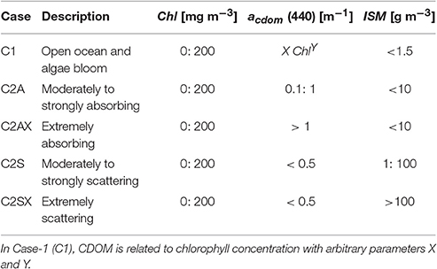
Table 1. Water case sub-classification that characterize the database in view of concentration ranges of chlorophyll, CDOM, and inorganic suspended matter.
Great variability of IOPs causes ambiguousness and therefore a significant degree of uncertainty in the interpretation of the remote sensing signal. We have to deal with a nonlinear and multivariate problem and the ocean color algorithm must be designed accordingly. The capability of bio-(geo)-optical algorithms strongly varies on global, regional, and very small scales and algorithms generally face more difficulties in Case-2 waters (e.g., Blondeau-Patissier et al., 2004; Darecki and Stramski, 2004; Gregg and Casey, 2004; Reinart and Kutser, 2006; Attila et al., 2013; Beltrán-Abaunza et al., 2014; Harvey et al., 2015). Indeed, it is a challenge to bridge the different scales with a high degree of reliability of the ocean color products. And we should not forget that marine atmospheric correction (AC), which is necessary to derive Rrs at the sea surface from satellite imagery and thus, provides input for in-water algorithms, is a complex task with additional uncertainties, in particular for extreme waters.
An artificial neural network (NN) is an appropriate regression technique to parametrize the inverse relationship between optical properties and reflectances. It has been proven in the last years that NNs produce reasonable approximations of ocean color products from optically complex (Case-2) waters. NNs have been applied to different satellite sensors in order to derive concentrations of water constituents, inherent and apparent optical properties (IOPs and AOPs), and photosynthetically available radiation (PAR), or to discriminate algae species (Gross et al., 1999; Schiller and Doerffer, 1999; D'Alimonte and Zibordi, 2003; Zhang et al., 2003; Tanaka et al., 2004; Schiller, 2006; Bricaud et al., 2007; Schroeder et al., 2007; Ioannou et al., 2011; Jamet et al., 2012; Chen et al., 2014; Hieronymi et al., 2015; D'Alimonte et al., 2016). Due to their speed, NN-based ocean color algorithms are deployed for operational and near-real time satellite observations, e.g., the MERIS Case-2 water algorithm (Doerffer and Schiller, 2007) and C2RCC (Brockmann et al., 2016).
The objective of this study is to introduce a new in-water processing scheme designed for OLCI ocean color observations called OLCI Neural Network Swarm (ONNS). The distinctive feature of this algorithm is its wide range of applicability in terms of optical water properties ranging from oligotrophic ocean waters to extremely turbid (scattering) or dark (absorbing) waters. The specific goals of the study are: (1) to reference the fundamental processing scheme, (2) to provide the scientific background, (3) to introduce the derived ocean color products, and (4) to evaluate the basic suitability of the algorithm for oceanic and coastal waters, i.e., C1, C2A, C2AX, C2S, and C2SX waters (Table 1).
ONNS Basis and Algorithm Description
ONNS is an in-water processor, which retrieves ocean color (OC) products from Sentinel-3 OLCI satellite scenes. Inputs to the algorithm are normalized remote sensing reflectances (just above the sea surface). Atmospheric correction is not part of the in-water processing scheme, and thus, ONNS fully relies on proper atmospheric correction (see Section Retrieval Accuracy). The processor logic is illustrated in Figure 1 and documented in the following.
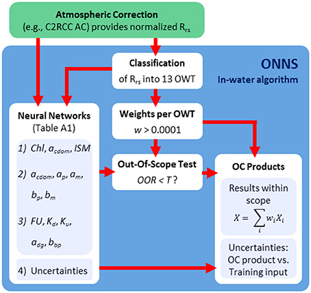
Figure 1. Flowchart of the OLCI Neural Network Swarm in-water ocean color processor.
Neural Network Algorithm
As it is the case for all ocean color algorithms, NNs are valid for a certain range of constituents and their concentrations, and some parameters may be deduced more accurately than others, e.g., retrieval of suspended matter is usually the least critical, whereas CDOM retrievals are the most challenging (Odermatt et al., 2012; Brewin et al., 2015). Our approach proposes to blend various NN algorithms, each optimized for a specific scope. This swarm of neural networks therefore, covers the largest possible variability of water properties including oligotrophic and extreme waters (Table 1).
Neural Network Data Basis
Basis for NN training is knowledge of the relationship between water constituents, i.e., their optical activity, and the spectral remote sensing reflectance, Rrs. The latter is defined as ratio between water-leaving (upwelling) radiance, Lw, and downwelling irradiance, Ed, both just above the water surface. For training and validation (test) purposes, a large (>105) dataset has been simulated using the commercial radiative transfer software Hydrolight (version 5.2; Sequoia Scientific, USA; Mobley, 1994). Hydrolight is a forward model to compute Rrs and many other light field-related quantities from optical specifications of the water body, such as specific absorption and scattering properties. Considered concentration ranges are defined in Table 1. Basis for estimating distributions, ranges, and covariances of optical parameters in the model are different in situ datasets: (1) primarily our data from the North and Baltic Sea (HZG), (2) OC-CCI (ESA, worldwide; Valente et al., 2016), (3) HELCOM (Baltic Sea 1997–2013; ICES, 2011), and (4) NOMAD (NASA, worldwide; Werdell and Bailey, 2005). The simulations cover the spectral range from 380 to 1,100 nm in 2.5 nm steps (hyperspectral over full VIS and NIR). Resulting reflectances and AOPs refer to a solar irradiation from zenith direction and nadir viewing angle, i.e., they are fully normalized. Many standard settings of Hydrolight are utilized (Mobley, 1994; Mobley and Sundman, 2013); specific inputs are defined in the following.
The total absorption contains fractions of absorption of pure water, phytoplankton pigments, minerals (also inorganic detritus or non-algae particles), and colored dissolved organic matter (CDOM, also referred as yellow substance or gelbstoff). The same distinction is made for scattering; only to CDOM no scattering is attributed. The absorption and scattering coefficients of pure water depend on temperature, salinity, and wavelength (data from WOPP v2 by Röttgers et al., 2016).
Phytoplankton absorption is determined by the composition and concentration of pigments, e.g., chlorophyll-a, Chl, which is generally used to quantify the marine biomass concentration. This means that different algae species have unique absorption spectra. Xi et al. (2015) showed the impact of chlorophyll-specific absorption spectra on Rrs. They identified five fundamental absorption shapes from which an inversion of algae species from remote sensing reflectance is possible. Figure 2A illustrates the basic chlorophyll-specific absorption, , spectra normalized at 440 nm that are utilized in this work (from Xi et al., 2015). Mixtures of these spectra represent the variability of spectral shapes that are found in measured data. It has been decided to combine two types of spectra, whereby one component dominates the signal with 80%. The globally most common spectral shape is labeled with “brown group”; it is very similar to the standard absorption spectrum used in Hydrolight and summarizes Heterokontophyta, Dinophyta, Haptophyta, and others that have a similar spectral shape. The “green group” includes Chlorophyta. Cyanobacteria are separated into blue (e.g., Aphanothece clathrata) and red (e.g., Synechococcus red) species. The two spectra for cyanobacteria are derived from in situ absorption measurements in the Baltic Sea. The three other spectra are taken from cultures. The phytoplankton (particle) absorption, ap, is related to the spectral chlorophyll-specific absorption and chlorophyll concentration, . The natural variability of phytoplankton absorption is very high (e.g., Bricaud et al., 2004) and included in the simulations (Figure 2B). Thus, when assessing Chl retrieval performance, this must be kept in mind.
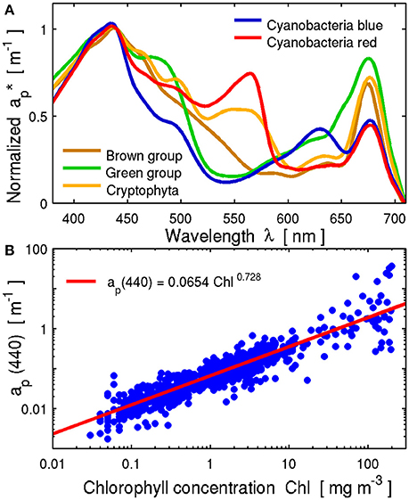
Figure 2. Bio-optical model of phytoplankton absorption. (A), Fundamental absorption spectra of five algae groups. (B), Modelled variability of the absorption coefficient of phytoplankton at 440 nm as function of chlorophyll concentration. The solid line shows the regression line of observations (Bricaud et al., 2004).
The shape of CDOM absorption is nearly exponential. Exponential functions have been used for C1 water simulations (Table 1). Here, CDOM absorption coefficients, acdom, and exponential slopes are varied strongly in order to display the natural variability (e.g., Valente et al., 2016). In addition, the present work uses modeled absorption spectra that are fitted to spectral measurements (by Rüdiger Röttgers, HZG). Based on this, further CDOM spectra are extrapolated toward ultra-extreme absorption with acdom(440) = 20 m−1. The exponential slope of these spectra (between 300 and 400 nm) is approximately 0.014 nm−1.
Fournier-Forand volume scattering functions have been applied for algae and non-algae particles (see Mobley and Sundman, 2013). The particle backscatter fraction, which actually correlates poorly with Chl and mineral (ISM) concentrations, is needed for the selection of appropriate phase functions. The corresponding formula of Twardowski et al. (2001) has been used for Chl-bearing particles. For inorganic particles, the mineral backscattering-ISM relationship of Zhang et al. (2010) has been utilized. The spectral mass-specific scattering coefficients are approximated by exponential functions, following the natural variability shown in measurements of organic-dominated and mineral-dominated waters (Woźniak et al., 2010).
The atmospheric and surface boundary conditions in Hydrolight are set constant, i.e., usage of the semi-empirical sky radiance model, assuming dry air with a marine aerosol type and moderate wind speed of 5 m s−1. The refractive index of water (as it is the case for absorption and scattering) is a function of water temperature (0–30°C) and salinity (0–35 PSU). The water is (virtually) infinitely deep. Effects of light polarization are not taken into account in Hydrolight.
All simulations have been carried out with and without inelastic scattering, i.e., Raman scattering, CDOM and Chl fluorescence, but without internal sources, i.e., no bioluminescence. In the end, data without inelastic scattering have been used for ONNS development. This is unproblematic in the selected setup with the 11 OLCI bands. Seen over the visible spectral range, differences mostly play no role, except for extreme absorbing waters, where high CDOM fluorescence is present. During algae bloom events, very high chlorophyll fluorescence peaks can be observed in nature (e.g., Fawcett et al., 2006), but modeling a certain quantum yield efficiency holds in itself great uncertainties (see Section ONNS Design). However, the simulations have been compared with observations and we generally have found a good agreement (Hieronymi et al., 2016). But we also have found some discrepancies partly related to plausible measuring uncertainties and possibly due to model simplifications.
NN Training
One part of the simulated dataset is put aside for later quasi-independent test purposes (see Section ONNS Application to Validation Data). The rest of the Rrs data is optically classified (Section Out-of-Scope Test) and grouped together. The scopes of concentrations together with median values are given in Table 2.
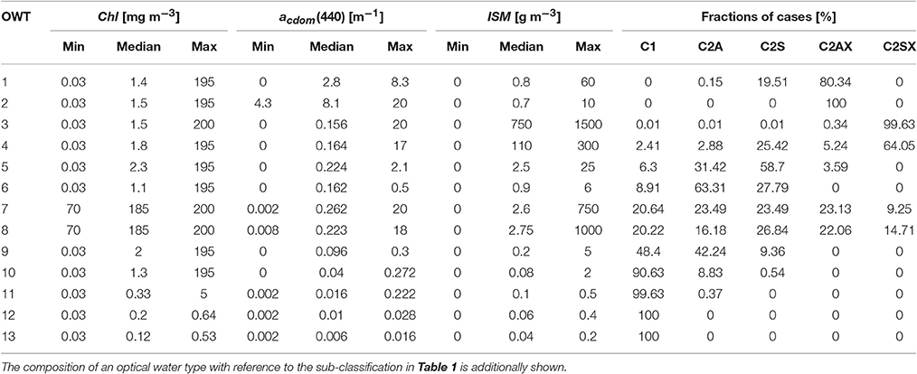
Table 2. Chlorophyll, CDOM, and inorganic suspended matter concentrations for the 13 optical water types.
The usable wavebands of the in-water algorithm are determined by the atmospheric correction at OLCI bands. We selected 11 (out of 21) OLCI wavebands for NN input (bands 1–8, 12, 16, and 17, i.e., at 400, 412.5, 442.5, 490, 510, 560, 620, 665, 755, 777.5, and 865 nm). The instrument's band widths vary and to be precise, the centers of bands 12 and 16 are actually at 753.75 and 778.75 nm respectively (Donlon et al., 2012). In contrast to other NN algorithms (e.g., Doerffer and Schiller, 2007), sun-viewing geometry is no input to the present NNs, instead input reflectances are normalized.
The selected output parameters are mostly common ocean color products (e.g., Nechad et al., 2015; Valente et al., 2016):
(1) Concentration of chlorophyll, Chl [mg m−3],
(2) Concentration of inorganic suspended matter (minerals), ISM [g m−3],
(3) Absorption coefficient of CDOM at 440 nm, acdom(440) [m−1],
(4) Absorption coefficient of phytoplankton particles at 440 nm, ap(440) [m−1],
(5) Absorption coefficient of minerals at 440 nm, am(440) [m−1],
(6) Absorption coefficient of detritus plus gelbstoff at 412 nm, adg(412) [m−1],
(7) Scattering coefficient of phytoplankton particles at 440 nm, bp(440) [m−1],
(8) Scattering coefficient of minerals at 440 nm, bm(440) [m−1],
(9) Total backscattering coefficient of all particles (organic and inorganic) at 510 nm, bbp(510) [m−1],
(10) Downwelling diffuse attenuation coefficient at 490 nm, Kd(490) [m−1],
(11) Upwelling diffuse attenuation coefficient at 490 nm, Ku(490) [m−1], and.
(12) Forel-Ule number, FU [-].
The 12 parameters are results of three independent sets of NNs, one that computes concentrations, one gives IOPs at 440 nm, and the last provides different IOPs and AOPs (see Appendix Table A1). Concentrations can be directly derived with NNs or alternatively, they can be estimated using IOPs, e.g., Chl from ap(440) or ISM from bm(440) (Doerffer and Schiller, 2007). The latter approach allows better adaptation of empirical relationships by means of in situ match-up data (which in case of OLCI is not yet available at present). All absorption and scattering contributions are retrieved at the reference wavelength 440 nm (pure water IOPs are known). Thereby, it is possible to estimate the total absorption, total scattering, and total attenuation coefficients. Mineral particles have usually lower absorption characteristics than CDOM, but shape-wise both are very similar. Following this reasoning, semi-analytical models, designed to retrieve IOPs from satellite data, often combine absorption by detritus (in this work only inorganic fraction) and gelbstoff (all water constituents which pass a filter pore size of 0.2 μm, which is often synonymous with CDOM). This absorption coefficient often corresponds to 412 nm. A similar idea holds true for the backscattering parameter. It is usually the backscattering coefficient of all marine particles together, which is measured in the field (at 510 nm). The diffuse attenuation coefficients are used to describe the attenuation of irradiance as a function of depth in water. It can be used to compute the depth of the euphotic zone. The Forel-Ule color scale was used for natural water classification long before the satellite era. In open ocean regions, the FU number is closely related to Chl concentration. Thus, the index can support ocean color trend analysis in the pre-satellite age and afterwards (Wernand et al., 2013; van der Woerd and Wernand, 2015). The color scale visualizes the color of the water body above a white Secchi disk that is hold at half Secchi depth.
A subsequent set of neural nets serves to evaluate the divergence of final OC products from the original training basis, i.e., Hydrolight simulations. The results are part of an uncertainty estimate (see Section Uncertainty Analysis).
The actual NN training procedure is described in Schiller and Doerffer (1999). The utilized multilayer feedforward-backpropagation neural net program is documented in Schiller (2000). The code was embedded in a program to test many NN architectures, i.e., varying numbers of hidden layers and neurons, and to optimize the learning process.
NN Scoring and Selection
Several hundreds of nets per water class and task with much different architecture have been produced. Afterwards, a ranking system has been applied in order to determine the optimal nets without over-training. In principle, statistical parameters such as root-mean-square error and goodness of fit are transformed into relative scores, which evaluate the quality of individual nets (Müller et al., 2015a). The best performing neural network architectures per water class are specified in Table A1. Inputs and outputs for the NNs are log10(X + 0.001), where X stands for Rrs or an ocean color product. The only exception is the Forel-Ule number, which is an integer between 1 and 21 and not logarithmized. The logarithmic form of input/output enables a distribution of values, which is closer to a uniform distribution within the range of input data, and therefore better approximation of outputs. The addition of 0.001 allows consideration of zero-values as input.
Fuzzy Logic Classification
Optical water type, OWT, classification based on remote sensing reflectance spectra has been developed to overcome the simplifications of Case-1 and Case-2 waters (Moore et al., 2001). It can bridge the gap between regionalized optical models and the global scale by combining several models according to their respective membership to a certain water type (Moore et al., 2009, 2012, 2014).
The classification is based on the simulated Rrs spectra (at 11 OLCI wavebands), but it is used for atmospheric corrected satellite data afterwards. Negative reflectances can occur after AC sometimes, while the spectral shape is still realistic. In order to avoid conflict with negative reflectances, the spectra are therefore transformed by log10(Rrs + 1) (note that Rrs is treated differently during classification and the NN application). Before the clustering, these transformed spectra are normalized by their brightness (sum of log-transformed reflectances), so that the classification is based on the shape of the spectrum alone. As the goal is to derive representative spectra, which have different spectral shapes and in particular a different spectral maximum, the sample from the simulation database does not take into account the frequency of natural occurrence of spectra. Spectra with their maximum at 510, 620, and 777.5 nm come in two distinctive shapes and there is no spectrum with maximum at 865 nm, so that during the agglomerative clustering 13 classes are selected. The 13 OWT classes are described by their class mean and standard deviation per wavelength of the brightness-scaled Rrs, which are used for the classification of spectra furthermore. The mean reflectance spectra of the 13 OWT classes are plotted in Figure 3.
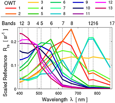
Figure 3. Brightness-scaled remote sensing reflectances for 13 classes of optical water types. Utilized OLCI bands are marked.
The five water type categories (Table 1) are defined by combinations of concentrations and thresholds. The water classes are designed to represent spectra, which have their maximum in the spectral shape at different wavelengths, independent of their brightness. Combining the water classes and the concentration categories is a test, which spectral shapes can be found in certain concentration ranges (Table 2).
Fuzzy set theory allows an element to have membership to one or more OWT classes (Moore et al., 2001). The weight of a class (membership function) is altered to allow for graded memberships, i.e., 0 ≤ wi ≤ 1, and to express partial class membership to the ith class. For constrained fuzzy sets the sum of all 13 weights equals 1. However, the class membership had to be above a minimum threshold, which was set at 0.0001. The membership to a class (weight) is calculated by determining the Mahalanobis distance between the given spectrum and the class means using the classes' covariance matrix respectively. Reconstruction of Rrs spectra by means of the fuzzy classification inversion yields mostly satisfying results. However, Rrs inversion from different atmospheric corrections reveals expected uncertainties in the violet-blue, which can be the case, if the satellite-acquired spectrum provided by the AC is distinctly different from modeled Rrs (which is basis of the classification).
Within the ONNS framework (Figure 1), the fuzzy logic classification scheme is used to assess the atmospheric corrected Rrs, and to determine the corresponding class memberships. The final blended retrieval for each pixel and each ocean color product is a weighted sum of the retrievals of all class-specific NNs (Appendix Table A1).
Out-of-Scope Test
Well-constructed NNs have good interpolation properties but produce unpredictable output when forced to extrapolate (Doerffer and Schiller, 2000). Therefore, measures have to be taken to recognize NN input not foreseen in the NN training phase and thus out of scope of the algorithm. Regarding simulated data, the fuzzy classification is well-constructed; maximum (or high) membership of a water class usually correlates well with the scopes of the corresponding NNs. However, it may happen that the classification yields a broad distribution of weights or that all memberships are such low that the spectrum is not classifiable. In the latter case, the satellite image pixel is flagged out. Despite the memberships, a quality measure is applied that evaluates the deviation of the NN input from the NN training range. The out-of-range parameter, OOR, is zero if the input is within the range but increases with increasing deviation. The assessment treats the input-reflectances spectrally differently; wavebands in the green spectral range have highest weights. The varying signal-to-noise specifications of OLCI are one argument for this (Donlon et al., 2012). Uncertainties in the fluorescence quantum yield efficiency of phytoplankton are another argument. Furthermore, we observe higher uncertainties in violet and blue wavebands generally shown in atmospheric correction validations (Müller et al., 2015a), but also from in situ determinations of Rrs due to the variable surface reflectance factor (Hieronymi, 2016; Zibordi, 2016). The allowance for OOR > 0 is one of the fine-tuning techniques to gain better spatial homogeneity of an OLCI scene and to adapt the algorithm to in situ observations.
Uncertainty Analysis
The determination of uncertainties of OC products is similar to the procedure applied in the C2RCC algorithm (Brockmann et al., 2016). All NNs per water class were reapplied to their training datasets to estimate the OC products. The uncertainty nets compare the estimated value, XE, with the initial training value, XT. The uncertainty per product is given as approximation (percent) error:
As it is the case for all OC products, the final approximation error is a weighted sum of the retrievals of all class-specific uncertainty NNs.
Test Data
Remote sensing reflectance data at OLCI wavelengths in conjunction with bio-geo-optical properties of the top water layer are used to evaluate the capacity of ONNS. For this purpose, different statistical parameters have been utilized. The degree of deviation is presented by the absolute root-mean-square error, RMSE. The Bias shows the average difference and is a measure for systematic over- or underestimation. Furthermore, the correlation coefficient, r, is calculated.
Simulated Data
Hydrolight-simulated data have been used to develop the classification scheme and to train neural nets. From the same data source (>105), a quasi-independent set of 23,445 reflectance spectra is used for testing and validation; these particular data are not used for ONNS development. The test data contain all water types from Table 1 and are shared approximately equally.
Simulated CCRR Data
A second synthetic dataset has been used to evaluate the performance of ONNS for the retrieval of water quality parameters. The “CoastColour Round Robin” (CCRR) dataset by Nechad et al. (2015) compiles inputs and results from 5,000 Hydrolight simulation. Atmospheric boundary conditions and simulation setup are comparable with above mentioned simulations. The used data refer to a sun zenith angle of 0°. Remote sensing reflectance at the 11 needed OLCI bands is interpolated from hyperspectral water-leaving reflectances between 350 and 900 nm with 5 nm steps. Corresponding Chl and ISM concentrations as well as CDOM absorption at 443 nm are tested with the ONNS retrieval (note that ONNS CDOM absorption coefficient refers to 440 nm).
In situ Data
Complete in situ datasets for the evaluation of OLCI-specific algorithms like ONNS are not freely available. The accessible data of CCRR (Nechad et al., 2015) and OC-CCI (Valente et al., 2016), which compiles data from several sources (e.g., MOBY, BOUSSOLE, AERONET-OC, NoMAD, MERMAID), lack of several Rrs bands. The ONNS algorithm needs only 11 out of 21 OLCI bands, but coinstantaneous data at 400, 755, 777.5, and 865 nm are not available. However, many of these sub-datasets are actually measured hyper-spectrally. Ramses radiometers, for example, that are deployed during our in situ campaigns, measure between 320 and 950 nm (TriOS optical sensors, Germany). Extracted multi-spectral reflectances together with Chl, ISM, and CDOM data are included in the CCRR in situ dataset; the corresponding measurement protocols are described in (Nechad et al., 2015). Our 48 data were collected between 2005 and 2006 (but not in winter) onboard a ferry from Cuxhaven to the island Helgoland in the German Bight (see Figure 5). Radiometric measurements were conducted under optimal sun-viewing angles (e.g., Zibordi, 2016), but strictly speaking, ONNS requires angle-normalized Rrs (with the sun in zenith) as input. Nonetheless, these data are used to test ONNS as well.
Sentinel-3 OLCI Scene
One Sentinel-3 OLCI scene is shown with permission to illustrate the qualitative and spatial application of ONNS (Figure 5). The tripartite scene was captured on 20 July 2016 between 9:30 and 9:36 UTC and shows large parts of the North and Baltic Sea. Thus, the scene images many different water types including different algae blooms. The satellite image indicates transparent cirrus clouds over the German Bight and Gulf of Finland, broken clouds over the Skagerrak and Kattegat, and cloud shadows. In comparison with MERIS, OLCI's view is slightly tilted in order to reduce the impact of sun glint, which is somewhat visible at the right edge of the image. Level-1 data of the first OLCI reprocessing are utilized for this work (IPF-OL-1-EO version 06.06). Atmospheric correction of the scene is provided by the C2RCC algorithm (“Case-2 Regional CoastColour,” version 0.15, Brockmann et al., 2016). An additional cloud mask was applied using the provided path radiance and viewing angles. At the same time of the satellite data acquisition, we measured Rrs in the German Bight for Sentinel-3 validation purposes (Figure 5), but these data are not used in this work.
Results
ONNS Application to Validation Data
The classification of simulated test data reveals that a maximum of four classes contribute to the inversion of Rrs spectra (the classes have non-zero weights). In principle, all water types (clear to extremely turbid) can be assigned properly. The classification failed on <3% of validation data; of those 56% are absorbing waters (C2A, C2AX) and approximately 70% have high Chl concentrations (Chl > 10 mg m−3). The classification of the in situ and simulated CCRR data yields no plausible results in approximately 10% of cases. The classifiable 4512 CCRR spectra exhibit maximum memberships in OWTs 1 (9%), 2 (0.5%), 4 (0.16%), 5 (55.2%), 6 (14.9%), 9 (10.6%), 10 (6.9%), 11 (1.7%), 12 (0.3%), and 13 (0.5%). Thus, a high percentage of these data correspond to the Case-1 or moderately to strongly scattering waters (Tables 1, 2). The 43 in situ data points, which are captured in coastal waters of the German Bight (Figure 5), have maximum memberships in OWT 1 (10.4%) and 5 (89.6%).
Examples of the retrieval capabilities of ONNS in comparison with validation data are illustrated in Figure 4. Estimates of concentration of Chl, ISM, and CDOM are shown for different water types, namely Case-1, extreme absorbing, and extreme scattering waters (Table 1). In addition, ONNS retrieval tests are shown for simulated data from the CCRR dataset and our in situ data. The colors characterize the estimated uncertainty in terms of the percent error. Green marks the generic ±5% uncertainty target for satellite ocean color products (defined for oligotrophic and mesotrophic Case-1 waters), orange and red colors signify an overestimation of the retrieved value in comparison with the expected (trained) value, and blue stands for an underestimation respectively. The uncertainty can be high in ambiguous cases with significant masking effects (in extreme waters) or if the NN data basis already provides high (natural) variability, as for example for Chl concentration (compare Figures 4A,D,G with Figure 2B). Despite high Chl variability, the uncertainty target can be achieved for all magnitudes of concentrations (varying over five orders of magnitudes), but with different occurrence in the water types: approximately 30% in C1, 10% in C2AX, and 5% in C2SX waters. An acceptance level of ±50% can be achieved in >97% of cases for C1, >80% in C2AX, and >70% in C2SX respectively. In all the cases, mean and median percentage errors are slightly negative, i.e., ONNS Chl retrieval shows a tendency for underestimation of expected values. Even if the test value is overestimated by ONNS, the uncertainty estimate may point to underestimation. This may be due to blending of NN from different OWT classes with distinctive different ranges of concentrations. In contrast to the simulated validation data, the ONNS Chl retrieval of CCRR and in situ data yields stronger deviations from the one-to-one line (Figures 4J,M).
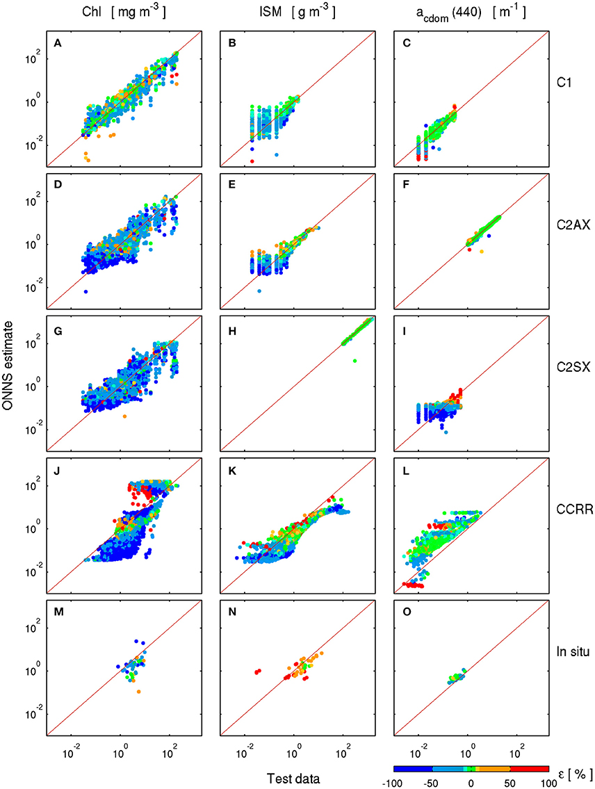
Figure 4. ONNS retrieval capacity for chlorophyll concentration (left), concentration of inorganic suspended matter (center column), and CDOM absorption at 440 nm (right) in comparison with simulated and in situ validation data. (A–C): Case-1 data from database, (D–F): Case-2 extreme absorbing waters, (G–I): Case-2 extreme scattering waters, (J–L): simulated data from CoastColour Round Robin (Nechad et al., 2015), (M–O): HZG in situ data. Colors indicate the retrieved uncertainty.
With regards to ISM, the retrieval performance is less skilled if the optical signal of minerals is weak due to low mineral concentrations—as it is the case in oligotrophic waters (Figure 4B). The 5% uncertainty target is reached within approximately 20% of all cases in C1 waters, 27% in C2AX, and >87% in C2SX. Thus, the more non-algae particles are present, the better ONNS performs. A similar trend can be observed for CDOM retrieval (Figures 4C,F,I). Lowest concentrations vanish in the noise, whereas high concentrations can be retrieved accurately. Approximately 60% target-retrievals can be achieved in C1 and >94% in extreme absorbing waters. Figure 4I illustrates the difficulties to separate the absorption signal due to CDOM and minerals; only 6% of estimates fall in the target-uncertainty range. In comparison to the Chl retrieval, ISM and CDOM retrievals of CCRR and in situ data show better agreement (Figures 4K,L,N,O).
The NN-estimated uncertainties and corresponding color distributions in Figure 4 reflect the comparative statistics that are tabulated for all water types (Table 3). Additional statistics of all OC products are listed in the (Table A2). With reference to the simulated test data and seen over all water types, the smallest differences between estimated and test data occur for the Forel-Ule number and both “mixed” IOPs, adg(412) and bbp(510). In comparison, larger deviations occur for low-concentration mineral-related values. We found weak water type-independent underestimation for the direct phytoplankton-related quantities [Chl, ap(440), and bp(440)] and for FU, Kd(490), Ku(490), adg(412), and bbp(510). But again, largest Biases are observed for the retrieval of non-algae properties in clear oceanic (almost mineral-free) C1 waters. The correlation coefficient reveals strong linear relationship for all cases exclusive of CDOM in extremely scattering waters, here the relation is weak (CDOM retrieval correlation is >0.95 for C2S and the other cases). The statistical values of the comparison with independent CCRR and in situ data paint a somewhat different picture with generally lower correlation coefficients (Table 3). Both datasets include turbid Case-2 waters that are predominantly characterized by one optical water type, i.e., OWT 5 (see Table 2). Most of the other water types are not independently evaluated.
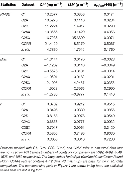
Table 3. Statistics of ONNS retrievals vs. test data.
ONNS Application to OLCI Scene
Application of the new ONNS algorithm to the satellite image is illustrated in Figure 6. Again, up to four optical water type classes are needed for the inversion. In this particular scene, water classes 3, 7, and 8 have no contribution to the products (all rather extreme turbid cases, see Table 2); all other classes give spatially dependent contributions (Figure 6A). Comparison with the mean shapes of the Rrs (Figure 3) meets regional expectations. In the western part of the Baltic Sea, including the Western Gotland Basin and the Bothnian Sea, the spectra show the strongest resemblance to classes 6, 9, and 10. Spectra of the Eastern Gotland Basin and Gulf of Finland fall into class 5 mostly and the Lagoons behind the Bay of Gdansk have some spectra with the shape of class 1. In contrast, we have found maximum memberships of classes 9, 10, and 11 in the clear open North Sea and Norwegian Sea and classes 1, 2, 4, 5, and 9 along the German and Dutch coasts. In some clear water cases (OWT 9, 10, and 11), the out-of-range warning flag for input spectra raises; these cases are mostly in spatial conjunction with transparent cirrus clouds (Figure 5). The Forel-Ule number that is estimated with ONNS provides an intuitively color impression and reconfirms expected geographic characteristics of the sea areas (Figure 6B).
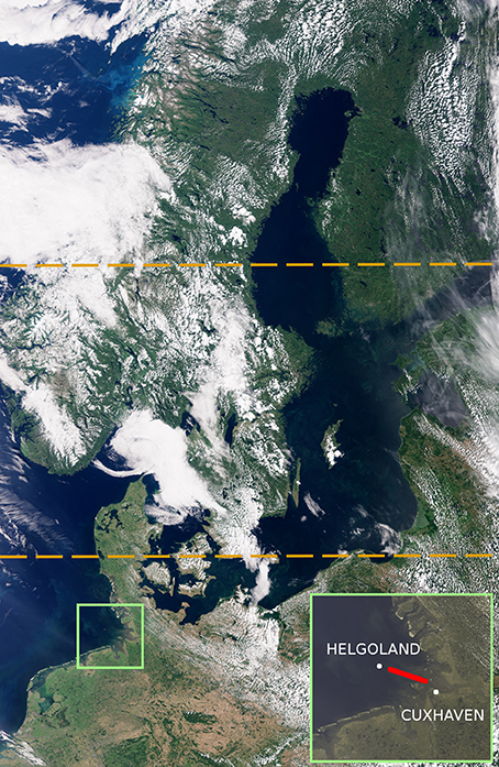
Figure 5. Sentinel-3 OLCI (top-of-atmosphere) scene of 20 July 2016 (contains modified Copernicus Sentinel data [2016] processed by ESA/EUMETSAT/HZG). The boundaries of individual scenes are marked with dashed lines. The picture detail shows the route with reflectance measurements in the German Bight.
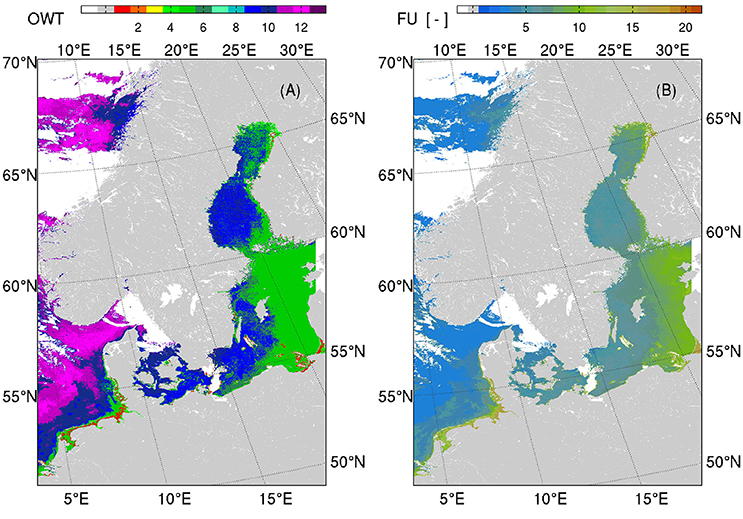
Figure 6. ONNS application to the OLCI scene (20 July 2016, Figure 5). (A): Optical water type classes with maximum membership. The gray color marks land areas, white shows the cloud mask above water and inland waters, and the other colors correspond to the spectra in Figure 3. (B): Retrieved Forel-Ule colors with true color impression.
Concentrations of Chl, ISM, and CDOM together with their accompanied uncertainty estimates are shown in Figure 7. Only valid sea pixels are shown; land areas and clouds are masked out. However, in spatial vicinity to clouds and coasts, apparently wrong assessments of OC products are possible; here, the predictions are overestimating the true values for the most part. Some areas are very shallow, e.g., the Curonian and Vistula Lagoons, and therefore, bottom reflections cannot be ruled out. This again would lead to possible overestimation of (particle) concentrations. All in all, the ranges of derived concentrations are reasonable (the colors on the left side of Figure 7 correspond to the respective units). Previous match-up analyses showed that most of the measured Baltic Chl values range between ~1 and 10 mg m−3 with somewhat smaller values in the Skagerrak-Kattegat region in comparison with the Central Baltic Sea (Pitarch et al., 2016). The ONNS-retrieved Chl values are in this range and reflect the geographic expectations (Figure 7A). But from the filamentous patterns it can be assumed that a cyanobacteria bloom including floating vegetation has developed in the Gotland Basin. In surface blooms, the concentrations are typically much higher, but the estimated biomass concentration seems too low. On the other hand, in some of these cases with visible algae structures, the out-of-range warning flag is raised (mostly OWT 9). Unfortunately, no in situ validation data of this OLCI image are available. The spatial distribution of ISM yields partly implausible features (Figure 7B). Commonly, significant concentrations of non-algae particles are not expected at the open sea. The concentration ranges, however, fit to observations by Berthon and Zibordi (2010). The regional distribution of CDOM, including the east-west gradient and high concentrations in the northern Baltic and Gulf of Finland, is plausible (e.g., Kowalczuk, 1999; Berthon and Zibordi, 2010; Ylöstalo et al., 2016). The corresponding uncertainty maps partly mirror the boundaries of the dominant water classes. Again, the high Chl uncertainties reflect the likewise high modeled variability (Figures 2B, 4, 7D).
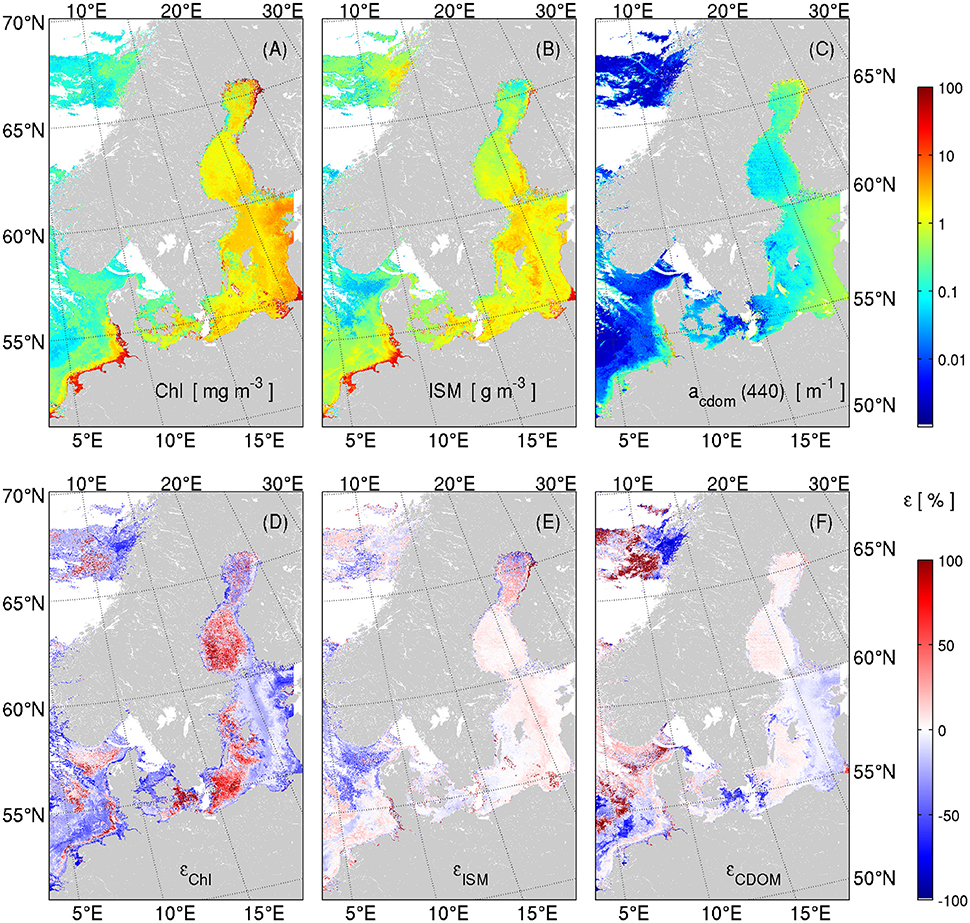
Figure 7. ONNS application to the OLCI scene (20 July 2016, Figure 5). (A–C): Upper panels show concentrations of chlorophyll, inorganic suspended matter, and CDOM (absorption coefficient at 440 nm). (D–F): The panels below show the corresponding retrieval uncertainties. Land and clouds are masked out.
ONNS application to contemporaneous Rrs measurements in the German Bight yield plausible results. All measured spectra exhibit maximum membership in OWT 5, the same as derived from the OLCI image for the transect (Figure 6A) and from 90% of the in situ data from the same area. The results are entirely in the same magnitudes as our previously measured in this area. ONNS estimates Chl along the transect between 1.7 and 4.5 mg m−3, ISM from 0.7 to 3.4 g m−3, and CDOM absorption (at 440 nm) between 0.38 and 0.68 m−1. Due to tides and hydrologic changes of the Elbe river plume, ISM can be higher than 10 g m−3 near the coast.
Discussion
Retrieval Accuracy
In general, the retrieval statistics of ONNS (Tables A1, A2, Figure 4) display the general problems of OC algorithms in the various water types (e.g., Blondeau-Patissier et al., 2004; Gregg and Casey, 2004; IOCCG, 2010; Odermatt et al., 2012; Brewin et al., 2015; Pitarch et al., 2016). All the more, one has to critically assess the quality of the Rrs input spectra, which is influenced by two factors: the sensor calibration (over which we have no control) and the atmospheric correction (AC). A careful atmospheric correction is of systematic importance for the success of the in-water algorithm—in particular for extreme Case-2 waters. Most of the light arriving at the satellite has been scattered by the atmosphere or reflected at the sea surface. The atmospheric path radiance is typically >85% of the total signal in C1 waters, >60% in C2SX, and >94% in C2AX waters (IOCCG, 2010). Existing AC processors address the various modeling aspects quite differently, e.g., the treatment of subvisible cirrus clouds or aerosol properties, and therefore, have strengths and weaknesses for specific water types (Müller et al., 2015a). In view of the new algorithm ONNS, which relies on normalized reflectances, angle-dependent AC processes such as “smile correction” and sun glint handling are important as well to ensure spatial homogeneity of satellite data. OLCI's viewing direction is slightly shifted in comparison with MERIS in order to reduce sun glint contaminated areas. However, some AC processors incorporate sun glint contributions in their reflectance models and derive normalized Rrs in this condition. These AC yield much larger coverage of data (Müller et al., 2015b), but areas with high glint should nevertheless be considered cautiously. One of the AC processors is Polymer (Steinmetz et al., 2011), which reveals good performance in comparison with MERIS match-ups (Müller et al., 2015a). Another processor is C2RCC (Case-2 Regional CoastColour; Brockmann et al., 2016), which is an evolution of the precursors “Case-2 Regional,” “ForwardNN,” and the “MERIS Case-2 water” algorithm (Doerffer and Schiller, 2007). C2RCC is available through ESA's Sentinel toolbox SNAP and it is used in the Sentinel-3 OLCI ground segment processor of ESA for generating Case-2 water products. Both Case-2 AC algorithms, Polymer and C2RCC, provide usable normalized Rrs at OLCI bands and give comparable memberships of OWT classes. Some differences between C2RCC and Polymer-derived Rrs are visible, mainly in the shape of the reflectance spectrum in the violet-blue spectral range. The sensor calibration especially for shorter wavelengths is subject to current investigations. Future versions of AC algorithms may incorporate the specific sensor properties. For this reason, we have to keep in mind that the results of ONNS to a certain degree rely on the applied atmospheric correction and data reprocessing version (subject to ongoing research).
One of the most important ocean color quantity is chlorophyll concentration. It is our general impression that ONNS delivers Chl in the expected orders of magnitude. Future tests must show the suitability of ONNS in comparison with other algorithms, globally and for the specific region (e.g., Blondeau-Patissier et al., 2004; Darecki and Stramski, 2004; Gregg and Casey, 2004; Attila et al., 2013). However, the Baltic Sea for example is known for intense cyanobacteria blooms with small-scale patches and extreme high biomass conditions (Chl > 200 mg m−3) partly associated with surface scums and floating algae. Under these conditions, results from different satellite sensors are very variable, values of Chl may exceed processing limits and atmospheric correction often fails (Reinart and Kutser, 2006). Optical properties of floating (also air bubble containing) material can be distinctly different from the data basis assumed in this work, e.g., higher backscattering and also higher reflectance in the NIR. Consequently, Rrs resembles dry vegetation rather than water (e.g., Kutser, 2004; Matthews et al., 2012), or—in terms of the defined optical water types—looks like (extreme) scattering waters. This means, as a corollary, that high biomass (Chl) is rather interpreted as non-algae particles (ISM). The out-of-range warning is notified for some of the affected areas. But here, it can be useful to raise an additional flag for surface scum conditions as it is suggested by Matthews et al. (2012). With regards to the possible misinterpretation of algae vs. non-algae particles, we must concede a potential weakness of the bio-geo-optical model assumptions underlying the simulated data basis. For example, the data include high variability of scattering properties but do not take scattering properties of different species into account (only chlorophyll-specific absorption), but it is likely that they are different (e.g., Harmel et al., 2016).
The selected OLCI scene is a good example for phytoplankton diversity. It is not well visible in Figure 5, but different algae blooms occur (none of them are confirmed). Very likely, a cyanobacteria bloom occurred in the Gotland Basin of the Baltic Sea. The bright water top left of the image along the Norwegian coast points to the occurrence of blooming coccolithophore. Moreover, west of the island Sylt in the German Bight fingerlike structures related to enhanced biomass are recognizable. The fact that we have to deal with different species within predominant water types increases the uncertainties. Chlorophyll-specific variability is included in the database for ONNS (Figure 2A). This and the high natural variability of phytoplankton absorption vs. Chl concentration are reflected in the uncertainty estimates of ONNS. On this basis, future developments of ONNS may be directed into optical differentiation of diversity with corresponding traceability of uncertainties (Bracher et al., 2017; Mouw et al., 2017).
It is a frequent practice to derive inherent optical properties from ocean color and from this create an empirical relationship to observed concentrations (e.g., Doerffer and Schiller, 2007). Besides the directly retrieved concentrations, ONNS provides a number of IOPs and AOPs. The nets which derive concentrations (Table A1, second column) must balance their estimates indirectly by means of the relationship between absorption and scattering properties. NNs that retrieve IOPs or AOPs can rather focus on either spectral reflectance reduction or enhancement, i.e., absorption or scattering. This is demonstrated by the statistical analysis shown in Table 3, A2. The correlation coefficients of estimated IOPs and AOPs are generally very high, even if we have to deal with cases of significant pigment absorption masking due to the influence of sediments. Once the spectrum is properly classified, the anticipated values are significantly restricted, which leads to high correlation. The derived sets of IOPs and AOPs form closure in a similar manner as the Hydrolight simulations, e.g., if we compare the sum of absorption and scattering coefficients at 440 nm (which is the attenuation coefficient) with the diffuse attenuation coefficient of downwelling irradiance, Kd(490), the correlation coefficient yields 0.856 for the test data and 0.841 for the ONNS-retrieved values, both seen over all water types. Due to the high input-variability of phytoplankton absorption vs. Chl concentration, we expect higher uncertainties related to the biomass concentration than related to other quantities as for example CDOM absorption (Figures 4, 7). The exploitation of various IOPs, e.g., absorption coefficient adg(412) or backscattering coefficient bbp(510), may lead to more accurate and regionalized OC products. Additionally, certain absorption or scattering properties may help identifying oceanographic features such as water masses or (sub-) mesoscale eddies and frontal systems (structures are best visible in total particulate backscattering). ONNS already is a regionally employable algorithm that delivers plausible outputs, and is thus in line with new multi-water type ocean color algorithms (e.g., D'Alimonte et al., 2014; Moore et al., 2014).
ONNS Design
The present version of the bio-geo-optical processing scheme applies 11 (from 21) OLCI bands (namely at 400, 412.5, 442.5, 490, 510, 560, 620, 665, 755, 777.5, and 865 nm). Wavebands that are affected by phytoplankton fluorescence (at 673.75, 681.25, and to only a minor degree at 708.75 nm) are not utilized. In principle, the inclusion of these bands could help the classification and Chl retrieval capacity, in particular for highly eutrophic waters. Admission of the three additional bands, also in the combined form of a fluorescence line height, slightly increases the accuracy of the Chl retrieval with respect to the simulated dataset, where inelastic scattering features with the standard settings of Hydrolight are included. But we have to keep in mind that fluorescence (quantum yield efficiency) is subject to strong fluctuations and potential false assessment; it has diurnal variability, depends on nutrient- and light-availability and algae species (e.g., Greene et al., 1994). The retrieval accuracy slightly decreases if the present fluorescence line height mismatches the expected range from the training dataset. Our tests show that this is less of a problem in case of in situ measured remote sensing reflectance, but deviations can be higher in case of atmospheric corrected satellite data (tested with C2RCC and Polymer). A proper atmospheric correction for these bands is difficult to achieve. For this reason, the Chl fluorescence bands are not used in the present version of the ONNS algorithm.
The main purpose of other OLCI NIR bands is atmospheric correction, e.g., due to oxygen and water vapor absorption and optical features of aerosols. Thus, satellite-derived Rrs is not provided for all of the NIR bands (Steinmetz et al., 2011). In contrast, many radiometers that are deployed for in situ Rrs determination measure hyper-spectrally in the VIS and NIR range (e.g., Ramses sensors). Hence, 20 OLCI bands (or more bands) could be theoretically used for a bio-geo-optical algorithm. The last OLCI band at 1,020 nm is not covered by many radiometers. For this reason and because of the little information gain in most waters, the 1,020 nm band was also not selected for ONNS input. However, we must bear in mind that available spectral bands in compiled in situ datasets (e.g., Nechad et al., 2015; Valente et al., 2016) are limited too, making meaningful validation difficult.
The new algorithm deploys Rrs that are angle-normalized, i.e., the sun is at zenith and the viewing direction is perpendicular. All sun and viewing angle-related effects must be eliminated by the atmospheric correction prior to ONNS application. The approach simplifies for example comparisons of different satellite sensors. The first step of the processing scheme is to transform the input Rrs into brightness-scaled reflectances. The advantage of this approach is that the classification is less sensitive to the amplitude of Rrs spectra, which can be shifted by various scattering processes, e.g., due to wind-dependent micro-bubbles in water (white scatterer), marine particle aggregation, particle size, or just under-estimation of the measured total scattering (e.g., McKee et al., 2013).
OWT Classification
The classification of synthetic validation data with same data source shows general good performance for most of the water types. Occasionally, in <3% of the validation data, the fuzzy classification yields no plausible memberships of the classes and thus no ONNS-retrieval values. Classification of very weak remote sensing reflectance signals, for example, is still challenging but mostly possible. The reason is that, e.g., in CDOM-rich lakes, the reflectance is near zero in almost the entire VIS, but nevertheless, significant phytoplankton biomass can be present (e.g., Kutser et al., 2016).
Fuzzy logic classification of the in situ and simulated CCRR validation data yields no significant memberships in approximately 10% of cases, i.e., in 5 and 488 cases respectively. Hence, the spectra were not considered plausible and the final blended retrieval delivers no results. One possible explanation is that spectral shapes of Rrs appear which not occur in the database with 105 spectra. Moore et al. (2001) propose a minimum threshold for class memberships, which was arbitrarily set at 10−4. If this threshold is lowered to 10−5, the non-plausible cases reduce to <1% of both datasets. Further tests are needed in the framework of an all-water-type-embracing validation.
Applied to a satellite scene, all marine spectra are classifiable, but water classification can be problematic and spatially heterogeneous in association with cloud and adjacency effects. Nonetheless, the optical water type classification of the scene basically yields geographically expected results. Three of the water classes (OWT 3, 7, and 8) gained never significant weights. Therefore, they were not used for blending. Those cases include extreme absorbing or scattering cases with very high biomass, e.g., like the mentioned “black lakes” (Kutser et al., 2016) or the Gulf of Finland (Ylöstalo et al., 2016), which is mostly flagged out due to clouds in the example scene. In global terms, they are restricted very locally. However, the three cases each represent a spectral Rrs with maxima in one of the three selected NIR bands (Figure 3); therefore, they have an essential function in the fuzzy logic classification scheme.
Application to Radiometric In situ Data
The OC processor ONNS can be applied to in situ measurements as well. In this case, an atmospheric correction is not needed. Remote sensing reflectance can be determined from above- or in-water radiometric measurements. Nechad et al. (2015) assembled reflectance measurements that are gained in five different manners. In case of above-water measurements for example, downwelling irradiance, sky radiance, and upwelling radiance are measured under specific sun-viewing angle conditions. From this, Rrs is determined using a surface reflectance factor, which depends on sun-viewing geometry and wind speed and which is usually between 2 and 5% for optimal viewing angles (Hieronymi, 2016; Zibordi, 2016). The surface reflectance factor determines the shape of Rrs mainly in the violet-blue range. Thus, there are some uncertainties for the application of the classification scheme and the overall processor. Optimally, the measured Rrs is adapted to the input criteria for ONNS, i.e., fully normalized, a moderate wind speed, no micro-bubbles in water, etc., In our tests, the fuzzy logic classification scheme is applicable and yields useable inputs for ONNS. Furthermore, ONNS retrieves OC products in the expected orders of magnitude. However, this cannot hide the fact that the retrieval statistic for the comparison with in situ data could be better (Table 3). Thus, more and all-water-type-embracing validation is needed.
Outlook
Proper validation of ONNS products using in situ data and OLCI match-ups will be a future task. Every OWT class must be validated (and possibly readjusted) independently, knowing that it is the balance between the water constituents (phytoplankton, minerals, and CDOM), represented in the training data, that decides on the quality of the OC products (D'Alimonte et al., 2016). Furthermore, higher validation uncertainties must be expected in extreme Case-2 waters and heterogeneous waters in coastal areas or during algae blooms (e.g., Kutser, 2004; Pahlevan et al., 2016). These in situ validation uncertainties must be incorporated into the delivered uncertainty products. The aim of this paper is to provide the scientific background description of the processor together with a baseline validation of the present ONNS version (v0.4). Once the processor has been validated, it is planned to make it freely accessible via ESA's Sentinel toolbox SNAP. After that, the algorithm will be compared with other bio-geo-optical algorithms.
In principle, ONNS can provide results in near-real time. The computational time depends on the (in our case high) number of neurons of the NNs and a swarm of 4 × 13 NNs obviously takes more time. However, single NNs are fast and the processing can occur in parallel. Thus, OC products can be disseminated in near real time mode, which usually comprises the time up to one day after satellite acquisition.
Conclusions
This study presents a novel in-water algorithm for the retrieval of ocean color remote sensing products from atmospheric corrected OLCI-like satellite imagery or in situ radiometric measurements. The algorithm consists of several specialized neural networks with task-optimized architectures (OLCI Neural Network Swarm). The products contain concentrations of water constituents (Chl and ISM), inherent and apparent optical properties [acdom(440), ap(440), am(440), adg(412), bp(440), bm(440), bbp(510), Kd(490), and Ku(490)], and a sea color index (FU). In addition, all products are delivered with an uncertainty estimate that describes the deviation of the product from the original data basis. The algorithm makes use of a comprehensive fuzzy logic classification scheme. Thirteen optical water type classes have been identified based on Hydrolight simulated and brightness-scaled remote sensing reflectances at 11 OLCI bands (400, 412.5, 442.5, 490, 510, 560, 620, 665, 755, 777.5, and 865 nm). The corresponding water types range from clearest sea waters to extreme Case-2 waters (Table 1). This includes chlorophyll concentrations up to 200 mg m−3, non-algae particle concentrations up to 1,500 g m−3, and an absorption coefficient of colored dissolved organic matter up to 20 m−1 at 440 nm. A baseline validation of ONNS products for the various water types is provided, showing principle strengths and weaknesses of the algorithm. With simulated test data the algorithm performs generally well within the wide range of optical properties of the water. Additional tests have been conducted using simulated data from the independent CCRR database and a few in situ data; both datasets contain mostly turbid Case-2 waters, which are classified in few optical water type classes. As might be expected, these comparisons revealed somewhat worse correlation but are overall encouraging, for example regarding ISM and CDOM retrieval. An appropriate full validation for all OWT classes and all provided ocean color products is still to be done. Conclusions on the performance using OLCI Earth observation data can be drawn after throughout validation against field measurements or other bio-geo-optical algorithms. The shown example demonstrates that ONNS-estimated ocean color products are mostly within the range of observed concentrations (e.g., Kowalczuk, 1999; Berthon and Zibordi, 2010; Pitarch et al., 2016; Ylöstalo et al., 2016). From our present point of view, we conclude that the new ONNS in-water algorithm is suited for the remote sensing estimation of water properties and constituents of most natural waters.
Author Contributions
MH and DM developed the concept of the processor ONNS with consultancy of RD. MH prepared the synthetic data basis, trained the neural networks, and wrote the paper. DM developed the water type classification, processed data, and contributed text modules. RD helped with the processor development and fed the discussion.
Funding
This work is a contribution to the European Space Agency (ESA) funded Ocean Colour Climate Change Initiative (OC-CCI: AO-1/6207/09/I-LG), Case-2 Extreme Water project (C2X: 4000113691/15/I-LG), and Living Planet Fellowship Programme (LowSun-OC: 4000112803/15/I-SBo).
Conflict of Interest Statement
The authors declare that the research was conducted in the absence of any commercial or financial relationships that could be construed as a potential conflict of interest.
Acknowledgments
This paper is an outcome of the CLEO Workshop “Colour and Light in the Ocean from Earth Observation,” held in Frascati, Italy in September 2016. The authors would like to acknowledge data processing and discussions with colleagues Rüdiger Röttgers, Hajo Krasemann, Kerstin Heymann, and Wolfgang Schönfeld. In addition, the authors thank the C2X project and science support team for valuable comments throughout the algorithm development, in particular Carsten Brockmann, Kerstin Stelzer, Ana Ruescas, François Steinmetz, Kevin Ruddick, Bouchra Nechad, Gavin Tilstone, Stefan Simis, and Peter Regner. We thank ESA/ EUMETSAT/ EU Copernicus for providing Sentinel-3 data and for permission to use them. Finally, the detailed comments of three reviewers and of the guest associate editor Tiit Kutser are highly appreciated.
References
Attila, J., Koponen, S., Kallio, K., Lindfors, A., Kaitala, S., and Ylöstalo, P. (2013). MERIS Case II water processor comparison on coastal sites of the northern Baltic Sea. Rem. Sens. Environ. 128, 138–149. doi: 10.1016/j.rse.2012.07.009
Beltrán-Abaunza, J. M., Kratzer, S., and Brockmann, C. (2014). Evaluation of MERIS products from Baltic Sea coastal waters rich in CDOM. Ocean Sci. 10, 377–396. doi: 10.5194/os-10-377-2014
Berthon, J. F., and Zibordi, G. (2010). Optically black waters in the northern Baltic Sea. Geophys. Res. Let. 37:L09605. doi: 10.1029/2010gl043227
Blondeau-Patissier, D., Tilstone, G. H., Martinez-Vicente, V., and Moore, G. F. (2004). Comparison of bio-physical marine products from SeaWiFS, MODIS and a bio-optical model with in situ measurements from Northern European waters. J. Optics A 6:875. doi: 10.1088/1464-4258/6/9/010
Bracher, A., Bouman, H., Brewin, R. J., Bricaud, A., Brotas, V., Ciotti, A. M., et al. (2017). Obtaining phytoplankton diversity from ocean color: a scientific roadmap for future development. Front. Mar. Sci. 4:55. doi: 10.3389/fmars.2017.00055
Brewin, R. J., Sathyendranath, S., Müller, D., Brockmann, C., Deschamps, P.-Y., Devred, E., et al. (2015). The ocean colour climate change initiative: III. a round-robin comparison on in-water bio-optical algorithms. Rem. Sens. Environ. 162, 271–294. doi: 10.1016/j.rse.2013.09.016
Bricaud, A., Claustre, H., Ras, J., and Oubelkheir, K. (2004). Natural variability of phytoplanktonic absorption in oceanic waters: influence of the size structure of algal populations. J. Geophys. Res. 109:C11010. doi: 10.1029/2004jc002419
Bricaud, A., Mejia, C., Blondeau-Patissier, D., Claustre, H., Crepon, M., and Thiria, S. (2007). Retrieval of pigment concentrations and size structure of algal populations from their absorption spectra using multilayered perceptrons. Appl. Opt. 46, 1251–1260. doi: 10.1364/AO.46.001251
Brockmann, C., Doerffer, R., Peters, M., Stelzer, K., Embacher, S., and Ruescas, A. (2016). “Evolution of the C2RCC neural network for Sentinel 2 and 3 for the retrieval of ocean colour products in normal and extreme optically complex waters,” in Proceeding of Living Planet Symposium (Prague: ESA SP-740).
Chen, J., Quan, W., Cui, T., Song, Q., and Lin, C. (2014). Remote sensing of absorption and scattering coefficient using neural network model: development, validation, and application. Rem. Sens. Environ. 149, 213–226. doi: 10.1016/j.rse.2014.04.013
D'Alimonte, D., Kajiyama, T., and Saptawijaya, A. (2016). Ocean color remote sensing of atypical marine optical cases. IEEE Trans. Geosci. Rem. Sens. 54, 6574–6586. doi: 10.1109/TGRS.2016.2587106
D'Alimonte, D., and Zibordi, G. (2003). Phytoplankton determination in an optically complex coastal region using a multilayer perceptron neural network. IEEE Trans. Geosci. Rem. Sens. 41, 2861–2868. doi: 10.1109/TGRS.2003.817682
D'Alimonte, D., Zibordi, G., Kajiyama, T., and Berthon, J. F. (2014). Comparison between MERIS and regional high-level products in European seas. Rem. Sens. Environ. 140, 378–395. doi: 10.1016/j.rse.2013.07.029
Darecki, M., and Stramski, D. (2004). An evaluation of MODIS and SeaWiFS bio-optical algorithms in the Baltic Sea. Rem. Sens. Environ. 89, 326–350. doi: 10.1016/j.rse.2003.10.012
Doerffer, R., and Schiller, H. (2000). Neural network for retrieval of concentrations of water constituents with the possibility of detecting exceptional out of scope spectra. in Proceedings IGARSS 2000. IEEE 2000 International, Vol. 2 (Honolulu), 714–717.
Doerffer, R., and Schiller, H. (2007). The MERIS Case 2 water algorithm. Int. J. Rem. Sens. 28, 517–535. doi: 10.1080/01431160600821127
Donlon, C., Berruti, B., Buongiorno, A., Ferreira, M. H., Féménias, P., Frerick, J., et al. (2012). The global monitoring for environment and security (GMES) sentinel-3 mission. Rem. Sens. Environ. 120, 37–57. doi: 10.1016/j.rse.2011.07.024
Fawcett, A., Bernard, S., Pitcher, G. C., Probyn, T. A., and du Randt, A. (2006). Real-time monitoring of harmful algal blooms in the southern Benguela. Afri. J. Mar. Sci. 28, 257–260. doi: 10.2989/18142320609504158
Greene, R. M., Kolber, Z. S., Swift, D. G., Tindale, N. W., and Falkowski, P. G. (1994). Physiological limitation of phytoplankton photosynthesis in the eastern equatorial Pacific determined from variability in the quantum yield of fluorescence. Limnol. Oceanogr. 39, 1061–1074. doi: 10.4319/lo.1994.39.5.1061
Gregg, W. W., and Casey, N. W. (2004). Global and regional evaluation of the SeaWiFS chlorophyll data set. Rem. Sens. Environ. 93, 463–479. doi: 10.1016/j.rse.2003.12.012
Gross, L., Thiria, S., and Frouin, R. (1999). Applying artificial neural network methodology to ocean color remote sensing. Ecol. Mod. 120, 237–246. doi: 10.1016/S0304-3800(99)00105-2
Harmel, T., Hieronymi, M., Slade, W., Röttgers, R., Roullier, F., and Chami, M. (2016). Laboratory experiments for inter-comparison of three volume scattering meters to measure angular scattering properties of hydrosols. Opt. Exp. 24, A234–A256. doi: 10.1364/oe.24.00a234
Harvey, E. T., Kratzer, S., and Philipson, P. (2015). Satellite-based water quality monitoring for improved spatial and temporal retrieval of chlorophyll-a in coastal waters. Rem. Sens. Environ. 158, 417–430. doi: 10.1016/j.rse.2014.11.017
Hieronymi, M. (2016). Polarized reflectance and transmittance distribution functions of the ocean surface. Opt. Exp. 24, A1045–A1068. doi: 10.1364/oe.24.0a1045
Hieronymi, M., Krasemann, H., Müller, D., Brockmann, C., Ruescas, A., Stelzer, K., et al. (2016). “Ocean Colour Remote Sensing of Extreme Case-2 Waters,” in Proceedings of Living Planet Symposium (Prague: ESA SP-740).
Hieronymi, M., Müller, D., Krasemann, H., Schönfeld, W., Röttgers, R., and Doerffer, R. (2015). “Regional ocean colour remote sensing algorithm for the Baltic Sea,” in Proceedings of Sentinel-3 for Science Workshop (Venice: ESA SP-734).
Ioannou, I., Gilerson, A., Gross, B., Moshary, F., and Ahmed, S. (2011). Neural network approach to retrieve the inherent optical properties of the ocean from observations of MODIS. Appl. Opt. 50, 3168–3186. doi: 10.1364/A.O.50.003168
IOCCG (2010). “Atmospheric correction for remotely-sensed ocean-colour products,” in Reports and Monographs of the International Ocean-Colour Coordinating Group, ed M. Wang (Dartmouth: IOCCG).
Jamet, C., Loisel, H., and Dessailly, D. (2012). Retrieval of the spectral diffuse attenuation coefficient Kd (λ) in open and coastal ocean waters using a neural network inversion. J. Geophys. Res. 117:C10023. doi: 10.1029/2012JC008076
Knaeps, E., Dogliotti, A. I., Raymaekers, D., Ruddick, K., and Sterckx, S. (2012). In situ evidence of non-zero reflectance in the OLCI 1020 nm band for a turbid estuary. Rem. Sens. Environ. 120, 133–144. doi: 10.1016/j.rse.2011.07.025
Kowalczuk, P. (1999). Seasonal variability of yellow substance absorption in the surface layer of the Baltic Sea. J. Geophys. Res. 104, 30047–30058. doi: 10.1029/1999JC900198
Kutser, T. (2004). Quantitative detection of chlorophyll in cyanobacterial blooms by satellite remote sensing. Limnol. Oceanogr. 49, 2179–2189. doi: 10.4319/lo.2004.49.6.2179
Kutser, T., Paavel, B., Verpoorter, C., Ligi, M., Soomets, T., Toming, K., et al. (2016). Remote sensing of black lakes and using 810 nm reflectance peak for retrieving water quality parameters of optically complex waters. Rem. Sens. 8:497. doi: 10.3390/rs8060497
Matthews, M. W., Bernard, S., and Robertson, L. (2012). An algorithm for detecting trophic status (chlorophyll-a), cyanobacterial-dominance, surface scums and floating vegetation in inland and coastal waters. Rem. Sens. Environ. 124, 637–652. doi: 10.1016/j.rse.2012.05.032
McKee, D., Piskozub, J., Röttgers, R., and Reynolds, R. A. (2013). Evaluation and improvement of an iterative scattering correction scheme for in situ absorption and attenuation measurements. J. Atmos. Oceanic Tech. 30, 1527–1541. doi: 10.1175/JTECH-D-12-00150.1
Mobley, C. D. (1994). Light and Water: Radiative Transfer in Natural Waters. New York, NY: Academic.
Mobley, C. D., Stramski, D., Bissett, W. P., and Boss, E. (2004). Optical modeling of ocean waters: is the Case 1-Case 2 classification still useful? Oceanography 17, 60–67. doi: 10.5670/oceanog.2004.48
Mobley, C. D., and Sundman, L. K. (2013). Hydrolight 5.2, Ecolight 5.2, Technical Documentation. Bellevue: Sequoia Scientific Inc.
Moore, T. S., Campbell, J. W., and Dowell, M. D. (2009). A class-based approach to characterizing and mapping the uncertainty of the MODIS ocean chlorophyll product. Rem. Sens. Environ. 113, 2424–2430. doi: 10.1016/j.rse.2009.07.016
Moore, T. S., Campbell, J. W., and Feng, H. (2001). A fuzzy logic classification scheme for selecting and blending satellite ocean color algorithms. IEEE Trans. Geosci. Rem. Sens. 39, 1764–1776. doi: 10.1109/36.942555
Moore, T. S., Dowell, M. D., Bradt, S., and Verdu, A. R. (2014). An optical water type framework for selecting and blending retrievals from bio-optical algorithms in lakes and coastal waters. Rem. Sen. Environ. 143, 97–111. doi: 10.1016/j.rse.2013.11.021
Moore, T. S., Dowell, M. D., and Franz, B. A. (2012). Detection of coccolithophore blooms in ocean color satellite imagery: a generalized approach for use with multiple sensors. Rem. Sens. Environ. 117, 249–263. doi: 10.1016/j.rse.2011.10.001
Morel, A., and Prieur, L. (1977). Analysis of variations in ocean color. Limnol. Oceanogr. 22, 709–722. doi: 10.4319/lo.1977.22.4.0709
Mouw, C. B., Hardman-Mountford, N. J., Alvain, S., Bracher, A., Brewin, R. W., Bricaud, A., et al. (2017). A consumer's guide to satellite remote sensing of multiple phytoplankton groups in the global ocean. Front. Mar. Sci. 4:41. doi: 10.3389/fmars.2017.00041
Müller, D., Krasemann, H., Brewin, R. J., Brockmann, C., Deschamps, P. Y., Doerffer, R., et al. (2015a). The ocean colour climate change initiative: I. A methodology for assessing atmospheric correction processors based on in-situ measurements. Rem. Sens. Environ. 162, 242–256. doi: 10.1016/j.rse.2013.11.026
Müller, D., Krasemann, H., Brewin, R. J., Brockmann, C., Deschamps, P. Y., Doerffer, R., et al. (2015b). The ocean colour climate change initiative: II. spatial and temporal homogeneity of satellite data retrieval due to systematic effects in atmospheric correction processors. Rem. Sens. Environ. 162, 257–270. doi: 10.1016/j.rse.2015.01.033
Nechad, B., Ruddick, K., Schroeder, T., Oubelkheir, K., Blondeau-Patissier, D., Cherukuru, N., et al. (2015). CoastColour Round Robin data sets: a database to evaluate the performance of algorithms for the retrieval of water quality parameters in coastal waters. Earth Syst. Sci. Data 7, 319–348. doi: 10.5194/essd-7-319-2015
Odermatt, D., Gitelson, A., Brando, V. E., and Schaepman, M. (2012). Review of constituent retrieval in optically deep and complex waters from satellite imagery. Rem. Sens. Environ. 118, 116–126. doi: 10.1016/j.rse.2011.11.013
Pahlevan, N., Sarkar, S., and Franz, B. A. (2016). Uncertainties in coastal ocean color products: impacts of spatial sampling. Rem. Sens. Environ. 181, 14–26. doi: 10.1016/j.rse.2016.03.022
Pitarch, J., Volpe, G., Colella, S., Krasemann, H., and Santoleri, R. (2016). Remote sensing of chlorophyll in the Baltic Sea at basin scale from 1997 to 2012 using merged multi-sensor data. Ocean Sci. 12, 379–389. doi: 10.5194/os-12-379-2016
Reinart, A., and Kutser, T. (2006). Comparison of different satellite sensors in detecting cyanobacterial bloom events in the Baltic Sea. Rem. Sens. Environ. 102, 74–85. doi: 10.1016/j.rse.2006.02.013
Röttgers, R., Doerffer, R., McKee, D., and Schönfeld, W. (2016). The Water Optical Properties Processor (WOPP): Pure Water Spectral Absorption, Scattering, and Real Part of Refractive Index Model, ATBD, Issue 1.8, ESA Water Radiance project.
Ruddick, K., De Cauwer, V., Park, Y. J., and Moore, G. (2006). Seaborne measurements of near infrared water-leaving reflectance: the similarity spectrum for turbid waters. Limnol. Oceanogr. 51, 1167–1179. doi: 10.4319/lo.2006.51.2.1167
Schiller, H., and Doerffer, R. (1999). Neural network for emulation of an inverse model operational derivation of Case II water properties from MERIS data. Int. J. Rem. Sens. 20, 1735–1746. doi: 10.1080/014311699212443
Schiller, K. (2006). Derivation of photosynthetically available radiation from METEOSAT data in the German Bight with neural nets. Ocean Dyn. 56, 79–85. doi: 10.1007/s10236-006-0058-1
Schroeder, T., Schaale, M., and Fischer, J. (2007). Retrieval of atmospheric and oceanic properties from MERIS measurements: a new Case-2 water processor for BEAM. Int. J. Rem. Sens. 28, 5627–5632. doi: 10.1080/01431160701601774
Steinmetz, F., Deschamps, P. Y., and Ramon, D. (2011). Atmospheric correction in presence of sun glint: application to MERIS. Opt. Exp. 19, 9783–9800. doi: 10.1364/OE.19.009783
Tanaka, A., Kishino, M., Doerffer, R., Schiller, H., Oishi, T., and Kubota, T. (2004). Development of a neural network algorithm for retrieving concentrations of chlorophyll, suspended matter and yellow substance from radiance data of the ocean color and temperature scanner. J. Oceanogr. 60, 519–530. doi: 10.1023/B:JOCE.0000038345.99050.c0
Twardowski, M. S., Boss, E., Macdonald, J. B., Pegau, W. S., Barnard, A. H., and Zaneveld, J. R. V. (2001). A model for estimating bulk refractive index from the optical backscattering ratio and the implications for understanding particle composition in case I and case II waters. J. Geophys. Res. 106, 14129–14142. doi: 10.1029/2000JC000404
Valente, A., Sathyendranath, S., Brotas, V., Groom, S., Grant, M., Taberner, M., et al. (2016). A compilation of global bio-optical in situ data for ocean-colour satellite applications. Earth Syst. Sci. Data 8, 235–252. doi: 10.5194/essd-8-235-2016
van der Woerd, H. J., and Wernand, M. R. (2015). True colour classification of natural waters with medium-spectral resolution satellites: seaWiFS, MODIS, MERIS and OLCI. Sensors 15, 25663–25680. doi: 10.3390/s151025663
Werdell, P. J., and Bailey, S. W. (2005). An improved in-situ bio-optical data set for ocean color algorithm development and satellite data product validation. Rem. Sens. Environ. 98, 122–140. doi: 10.1016/j.rse.2005.07.001
Wernand, M. R., van der Woerd, H. J., and Gieskes, W. W. (2013). Trends in ocean colour and chlorophyll concentration from 1889 to 2000, worldwide. PLoS ONE 8:e63766. doi: 10.1371/journal.pone.0063766
Woźniak, S. B., Stramski, D., Stramska, M., Reynolds, R., Wright, V. M., Miksic, E. Y., et al. (2010). Optical variability of seawater in relation to particle concentration, composition, and size distribution in the nearshore marine environment at Imperial Beach, California. J. Geophys. Res. 115:C08027. doi: 10.1029/2009jc005554
Xi, H., Hieronymi, M., Röttgers, R., Krasemann, H., and Qiu, Z. (2015). Hyperspectral differentiation of phytoplankton taxonomic groups: a comparison between using remote sensing reflectance and absorption spectra. Rem. Sens. 7, 14781–14805. doi: 10.3390/rs71114781
Ylöstalo, P., Seppälä, J., Kaitala, S., Maunula, P., and Simis, S. (2016). Loadings of dissolved organic matter and nutrients from the Neva River into the Gulf of Finland–Biogeochemical composition and spatial distribution within the salinity gradient. Mar. Chem. 186, 58–71. doi: 10.1016/j.marchem.2016.07.004
Zhang, M., Tang, J., Song, Q., and Dong, Q. (2010). Backscattesring ratio variation and its implications for studying particle composition: a case study in Yellow and East China seas. J. Geophys. Res. 115:C12014. doi: 10.1029/2010jc006098
Zhang, T., Fell, F., Liu, Z. S., Preusker, R., Fischer, J., and He, M. X. (2003). Evaluating the performance of artificial neural network techniques for pigment retrieval from ocean color in Case I waters. J. Geophys. Res. 108:3286. doi: 10.1029/2002jc001638
Zibordi, G. (2016). Experimental evaluation of theoretical sea surface reflectance factors relevant to above-water radiometry. Opt. Exp. 24, A446–A459. doi: 10.1364/oe.24.00a446
Appendix
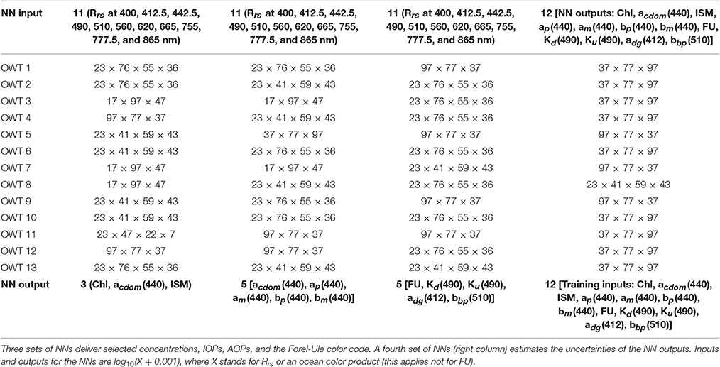
Table A1. Numbers of neurons from selected neural network architectures (input, hidden, and output layers) for all 13 optical water type classes.
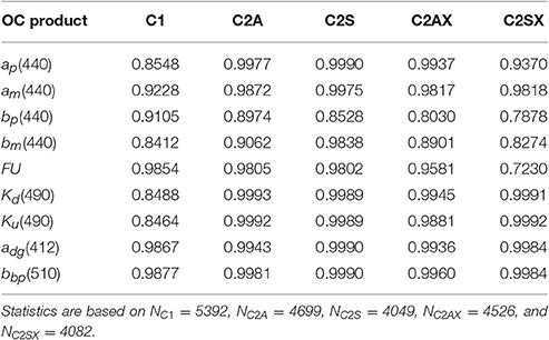
Table A2. Correlation coefficients of additional ONNS retrievals vs. simulated validation data subdivided by water type.
Keywords: ocean color, remote sensing, Sentinel-3, OLCI, extreme Case-2 waters, neural network, fuzzy logic classification
Citation: Hieronymi M, Müller D and Doerffer R (2017) The OLCI Neural Network Swarm (ONNS): A Bio-Geo-Optical Algorithm for Open Ocean and Coastal Waters. Front. Mar. Sci. 4:140. doi: 10.3389/fmars.2017.00140
Received: 15 December 2016; Accepted: 26 April 2017;
Published: 11 May 2017.
Edited by:
Tiit Kutser, University of Tartu, EstoniaReviewed by:
Tim Moore, University of New Hampshire, USAJenni Attila, Finnish Environment Institute, Finland
Mark Matthews, CyanoLakes, South Africa
Copyright © 2017 Hieronymi, Müller and Doerffer. This is an open-access article distributed under the terms of the Creative Commons Attribution License (CC BY). The use, distribution or reproduction in other forums is permitted, provided the original author(s) or licensor are credited and that the original publication in this journal is cited, in accordance with accepted academic practice. No use, distribution or reproduction is permitted which does not comply with these terms.
*Correspondence: Martin Hieronymi, bWFydGluLmhpZXJvbnltaUBoemcuZGU=
†Present Address: Dagmar Müller, Brockmann Consult GmbH, Geesthacht, Germany