 Lennart T. Bach1*
 Nauzet Hernández-Hernández2
 Jan Taucher1
 Carsten Spisla1
 Claudia Sforna1
 Ulf Riebesell1
 Javier Arístegui2
- 1Biological Oceanography, GEOMAR Helmholtz Centre of Ocean Research Kiel, Kiel, Germany
- 2Instituto de Oceanografía y Cambio Global, Universidad de Las Palmas de Gran Canaria, Las Palmas, Spain
Diatoms are silicifying phytoplankton contributing about one quarter to primary production on Earth. Ocean acidification (OA) could alter the competitiveness of diatoms relative to other taxa and/or lead to shifts among diatom species. In spring 2016, we set up a plankton community experiment at the coast of Gran Canaria (Canary Islands, Spain) to investigate the response of subtropical diatom assemblages to elevated seawater pCO2. Therefore, natural plankton communities were enclosed for 32 days in in situ mesocosms (∼8 m3 volume) with a pCO2 gradient ranging from 380 to 1140 μatm. Halfway through the study we added nutrients to all mesocosms (N, P, Si) to simulate injections through eddy-induced upwelling which frequently occurs in the region. We found that the total diatom biomass remained unaffected during oligotrophic conditions but was significantly positively affected by high CO2 after nutrient enrichment. The average cell volume and carbon content of the diatom community increased with CO2. CO2 effects on diatom biomass and species composition were weak during oligotrophic conditions but became quite strong above ∼620 μatm after the nutrient enrichment. We hypothesize that the proliferation of diatoms under high CO2 may have been caused by a fertilization effect on photosynthesis in combination with reduced grazing pressure. Our results suggest that OA in the subtropics may strengthen the competitiveness of (large) diatoms and cause changes in diatom community composition, mostly under conditions when nutrients are injected into oligotrophic systems.
Introduction
Diatoms are a group of globally distributed phytoplankton, with an estimated contribution of ∼25% to global primary production (Nelson et al., 1995; Field et al., 1998; Tréguer and De La Rocha, 2013). All diatom species share the trait of protecting the organic part of the cell with a shell (frustule) made of amorphous silica (opal), probably to reduce grazing pressure (Hamm and Smetacek, 2007; Pondaven et al., 2007; Friedrichs et al., 2013; Liu et al., 2016). To form the frustule, diatoms require dissolved silicate as an additional nutrient, which is often limiting in seawater and hence limiting their proliferation (Brzezinski and Nelson, 1996). Diatoms are strong competitors and typically dominate phytoplankton communities early in the succession when nutrients are sufficiently available (Sarthou et al., 2005).
There are at least 30,000 extant diatom species which span a size range from under 3 micro- up to a few millimeters (Mann and Vanormelingen, 2013). They occur as single cells or cell chains in benthic and/or pelagic habitats, and have free-living, surface-associated, symbiotic, or parasitic lifestyles (Armbrust, 2009; Mann and Vanormelingen, 2013).
Changes in diatom community composition can reorganize the flux of elements in oceans and the flow of energy within food webs (Armbrust, 2009; Tréguer et al., 2018). For example, particulate organic carbon sequestration to the deep ocean was shown to be 1.8 times higher in 1989 when the North Atlantic spring bloom was dominated by a larger species compared to the following year when smaller ones dominated (Boyd and Newton, 1995). Likewise, energy transfer to higher trophic levels is likely to be more efficient in assemblages where primary production is dominated by larger diatoms since less trophic intermediates are involved (Sommer et al., 2002). Thus, it is essential to determine how diatom community composition could be affected by different environmental stressors and in different ocean regions due to their enormous relevance for the Earth system.
In the present study we investigated how ocean acidification (OA) – the anthropogenic perturbation of seawater carbonate chemistry – could affect the composition of natural diatom communities in the subtropical NE Atlantic. Therefore, we set up a mesocosm experiment at the coast of Gran Canaria and perturbed the enclosed plankton communities with different CO2 concentrations. In the study region, diatom blooms often occur in association with meso-/sub-mesoscale structures such as upwelling filaments, zonal fronts, or eddies which inject nutrients into the euphotic zone (Barton et al., 1998; Arístegui et al., 2004; McGillicuddy et al., 2007; Anabalón et al., 2014). To account for this, the mesocosms were enriched with inorganic nutrients (N, P, Si) halfway through the experiment. This allowed us to investigate CO2 effects on diatoms during oligotrophic conditions (phase I) and during a subsequent nutrient injection to the euphotic zone (phase II).
Materials and Methods
Mesocosm Design, Deployment, and Maintenance
On February 23, 2016, we deployed eight in situ mesocosms (M1–M8) at the pier of Taliarte harbor, on the eastern coast of Gran Canaria (Canary Islands, 27° 59′ 24″ N, 15° 22′ 8″ W). The cylindrical mesocosm bags (Ø 2 m, 2.5 m long) were made of transparent polyurethane foil (PU), which is also used for the larger version of the KOSMOS mesocosm design (Riebesell et al., 2013). The PU bags were installed in a floatation frame made of polyethylene with steel reinforcements and deployed inside the harbor (Figure 1). The floatation frame was fixed on the pier and on mooring weights on the water side. A pulley system attached to the mooring weights allowed us to move the entire structure ∼2 m away from the pier in between samplings. This was necessary to reduce the influence of the pier on the light environment inside the mesocosms.
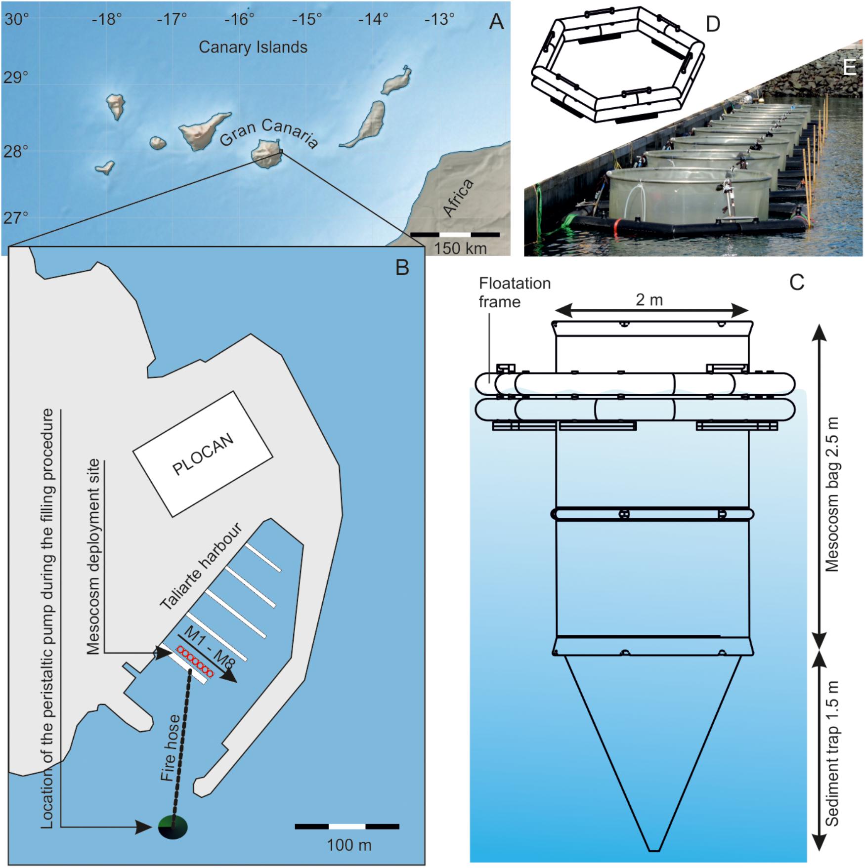
Figure 1. Study site and mesocosm setup. (A) Map of the Canary Islands in the subtropical North Atlantic. (B) Close-up on Taliarte harbor at the east coast of Gran Canaria. Mesocosms were installed in a row near a floating ponton and filled at the beginning of the study with water pumped into the bags from outside the harbor. (C) Technical drawing of one mesocosm and (D) a floatation frame. (E) Photograph of the mesocosm position during sampling. Please note that all mesocosms were only attached to the ponton during the ∼3 h samplings but positioned two meters away from the ponton for the rest of the time.
Conical sediment traps were attached to the bottom of the bags, thereby creating 8 isolated volumes (Figure 1). The sediment traps were 1.5 m long and similar to the KOSMOS design (Boxhammer et al., 2016). The mesocosms were initially empty and filled in the morning of March 2 by pumping seawater from ∼30 m outside Taliarte harbor into the enclosures (Figure 1). Seawater was pumped with a peristaltic pump from 3 to 5 m depth through a hose (Ø 50 mm with a 3000 μm mesh attached to the inlet) into a central volume on the pier, from where the seawater was simultaneously distributed with separate hoses (Ø 37 mm) into the mesocosms. The entire filling procedure lasted ∼4.5 h, and we tried to keep the stress level for pumped organisms low by restricting the speed of the peristaltic pump (3.9 L/s). We cannot fully ensure, however, that particularly sensitive organisms weren’t harmed and excluded from the experiment. Each mesocosm contained a volume of ∼8 m3 after filling. The filling marks the beginning of the experiment and is hereafter referred to as day –3, while day 0 is the day when the CO2 manipulation started (see section “Experimental Design”).
The mesocosm PU foil must be cleaned on a regular basis to avoid the growth of benthic organisms and to maintain light transmission. The outer sides of the mesocosm bags were cleaned by divers with brushes on days 6, 14, 17, and 25. The inner sides were cleaned on days 6, 14, 18, and 25 with a custom made cleaning ring which has approximately the same diameter as the mesocosm bags and thoroughly wipes the foil while sliding downward (Riebesell et al., 2013). The sediment traps were cleaned from the inside on day 15 with custom made “magnetic brushes” since the cleaning ring could not reach this part of the mesocosms. The magnetic brushes are basically two brushes that connect through the PU foil with a magnet and are operated from the outside by divers.
M1 was damaged early in the experiment (day 4) and therefore excluded from the analysis.
Experimental Design
A gradient of 7 CO2 concentrations (ambient to on average ∼1140 μatm) was established in 3 steps over 3 days (day 0 until day 2) by adding differential amounts [between 35 L (M7) and 70 L (M6)] of CO2-saturated seawater evenly to the water columns of M2–M8 with a custom-made distribution device (Riebesell et al., 2013). M5 was left unperturbed and served as a control but received non-aerated seawater during CO2 manipulations. CO2-saturated seawater had to be added at regular intervals during the experiment (days 6, 8, 10, 14, 18, and 25) to counteract CO2 outgassing at the surface. On day 18, we added NaNO3, Na2HPO4, and Na2SiO3 (3.43 ± 0.32, 0.16 ± 0.01, 1.63 ± 0.12 μmol L-1, mean ±SD between mesocosms) to each mesocosm to simulate an upwelling event of nutrient rich deep-water.
Sampling
Sinking detritus is collected in the terminal end of the sediment trap and removed from there through a hose connected to a vacuum system (Boxhammer et al., 2016). Sediment traps were emptied every second day to avoid resuspension and anoxic conditions at the bottom of the mesocosms.
Water samples from each mesocosm were collected between 9:00 and 11:00 a.m., either every second day (day -2–17 and 25–29) or daily (day 19–25) to obtain higher temporal resolution right after nutrient fertilization. Sampling was slightly later on day -3 (1:00–2:30 p.m.) since we wanted to have samples directly after filling the mesocosms with seawater. As sampling gear, we used 2.5 m long polypropylene pipes equipped with a pulley system to close the tube at the upper and the lower end. The pipe was left open on both ends and carefully lowered vertically into the water column until the lower end reached a depth of 2.5 m. The upper and the lower end were then closed from the surface with the pulley system, thereby enclosing a vertically integrated water sample. The integrated sample was gently mixed and transferred from the pipes into different sampling bottles. Between 3 and 5 hauls with the pipes were made to sample enough volume for all measurements.
Samples for dissolved inorganic carbon (DIC), total alkalinity (TA), and dissolved inorganic nutrient concentrations [NO3- + NO2-, NH4+, PO43-, Si(OH)4] were transferred directly from the sampling tubes into air-tight 1 L polycarbonate (carbonate chemistry) and 0.25 L polyethylene (PE) bottles (nutrients), respectively. DIC samples were carefully transferred in the 1 L bottles allowing considerable overflow before closing them with negligible headspace (i.e., <1 mL). Both carbonate chemistry and nutrient samples were transported in a cooling box to the land-based laboratories of the Plataforma Oceánica de Canarias (PLOCAN) which is located next to Taliarte harbor and hosted our study (Figure 1). DIC and TA samples were pumped from the 1 L bottles through a syringe filter (0.2 μm, Whatman) into air-tight 50 mL glass bottles (DIC) and 100 mL PE bottles (TA, nutrients), respectively. We allowed considerable overflow before closing the DIC glass bottles to minimize gas exchange. Filtered DIC, TA, and nutrient samples were stored at 4°C until analysis on the same day.
The seawater used to measure chlorophyll a (chla) and biogenic silica (BSi) concentrations, as well as diatom cell abundance, was carefully transferred from the sampling tubes into 10 L PE carboys and transported into a climate chamber at PLOCAN set to 15°C. Chla and BSi samples were tapped from the carboys (0.5–0.2 L depending on concentration), filtered (Δpressure = 200 mbar) on glass fiber filters (chla, GF/F nominal pore size = 0.7 μm) or cellulose acetate filters (BSi, pore size = 0.65 μm), and stored at -20°C until analysis. Microscopy samples were transferred from the carboys in 200 mL brown glass bottles, fixed with acidic Lugol solution (1% final concentration), and stored for maximally 5 months at room temperature until analysis.
Mesozooplankton (MesoZP) samples were collected every 4 days between 11 a.m. and 1 p.m. with vertical net hauls from 2.5 m to the surface. Sampling was carried out with a 0.6 m long Apstein net (55 μm mesh size), which had a 0.09 m diameter cone-shaped opening. Two consecutive net hauls per mesocosm during every sampling resulted in a sample volume of 32 L for each mesocosm.
Temperature (T) and salinity (S) were measured on every sampling day around noon time with a hand-held self-logging CTD probe (CTD60M, Sea and Sun Technologies). Average T and S were calculated by averaging the vertical profile from the surface (0.3 m) to the bottom of the sediment traps (∼3.5 m).
Analytical Procedures
NO3- + NO2- (NOx-), PO43- (P), and Si(OH)4 (Si) concentrations were measured photometrically within 10 h after sampling (Hansen and Koroleff, 1999). NH4+ concentrations were measured fluorometrically in the same timeframe (Holmes et al., 1999). Precision of nutrient measurements was generally well below ±10% as determined with triplicate measurements of each sample. DIC concentrations were measured within 10 h after sampling with an Autonomous Infra-Red Inorganic Carbon Analyser (AIRICA) system (Marianda, Kiel, Germany). Each sample was measured three times and the precision was in most cases better than ±3 μmol kg-1. TA was determined in an open cell titration within 24 h after sampling (Dickson et al., 2003). Each sample was measured twice with a precision that was in most cases better than ±4 μmol kg-1. Both DIC and TA measurements were accuracy-controlled by measurements of certified reference materials (Dickson et al., 2007). pCO2 partial pressure was calculated from measured (water-column averaged) temperature and salinity, as well as concentrations of DIC, TA, PO43- and Si(OH)4 using Seacarb (Lavigne et al., 2011). We used the recommended default setting and the carbonate dissociation constants (K1 and K2) determined by Lueker et al. (2000). Chla was extracted 1–2 days after sampling in acetone (90%) in plastic vials, by homogenization of the filters using glass beads and a cell mill (5 min). After centrifugation (10 min, 800 g, 4°C), the supernatant was analyzed on a fluorometer (TURNER 10-AU) following Welschmeyer (1994). The fluorometer was calibrated with spinach chla extract as described by Strickland and Parsons (1972). BSi concentrations were determined by leaching the samples with 0.1 M NaOH for 135 min at 85°C. The leaching process was terminated with 0.05 M H2SO4 and dissolved silicate was measured by spectrophotometry following Hansen and Koroleff (1999).
Diatom samples were transferred from the brown glass sampling bottles into 25–100 mL Utermöhl chambers. After at least 24 h of sedimentation, cells were counted with an inverted light microscope (Zeiss Axiovert 100). Cells were classified to the lowest identifiable taxonomical level. Diatom cell volumes were estimated following Olenina et al. (2006). We tried to measure the relevant shape dimensions needed for the geometrical formulas but in cases where this was not possible we used species dimensions provided by Olenina et al. (2006) (see Table 1). Carbon biomasses of individual species (μg C L-1) were calculated with the volume to carbon transfer functions provided by Menden-Deuer and Lessard (2000). Diatom diversity was estimated with the Shannon Weaver diversity index (H’):
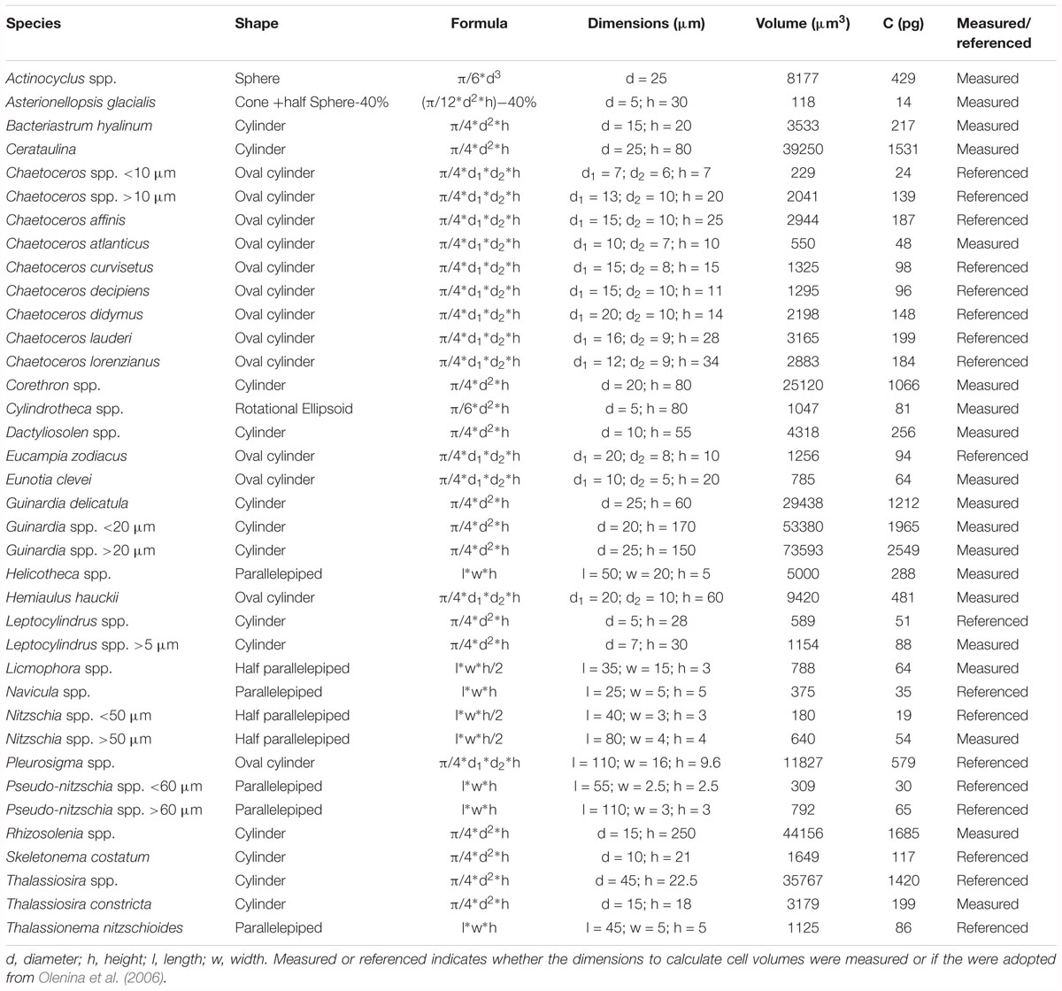
Table 1. List of all diatom species enumerated by means of light microscopy.
where Bi is the C biomass of diatom species i and Btotal the C biomass of all diatoms. Higher H’ is equivalent to a higher diversity.
The average cellular carbon quota (Cq) of the diatom community was calculated as:
where Ci is the carbon content of diatom species i, Ni is the abundance of diatom species i, and Ntotal is the abundance of all diatoms.
MesoZP was preserved with ethanol (70%) and transferred into a Bogorov counting chamber where it was quantified and classified to the lowest possible taxonomic level using a Leica stereomicroscope (MZ12). Copepodites and adult copepods of each species were counted as separate categories but we pooled them for our analysis. Accordingly, MesoZP abundances shown in this paper are copepodites + adults for each species. Nauplii species were not distinguished and counted as one group.
Data Analyses
To analyze the dataset, we split the experiment into 3 consecutive phases. Phase 0 was the time before the CO2 manipulation (day -3–day -1). Phase I (day 0–day 17) comprised the oligotrophic conditions that prevailed prior to the nutrient addition on day 18. Phase II (day 19–day 29) comprised the phytoplankton bloom that formed under eutrophic conditions after nutrient fertilization. For the analyses we calculated the phase averages of pCO2 (i.e., the independent variable) and the phase averages of the various dependent variables (e.g., chla or BSi). Shapiro-Wilk tests revealed non-normal distribution of the datasets so that they were log-transformed. Afterward, we ran regression analyses with the log-transformed data using R1 as in Schulz et al. (2013) and Paul et al. (2015). CO2 was considered to influence the abundance of individual diatom species when we detected a significant (p < 0.05) correlation between pCO2 and diatom abundance.
Dissimilarities in diatom community composition between CO2 levels were mapped by means of Principal Coordinate Analyses (PCoA) using C biomass data (μmol C L-1) from the most important diatom genera: Guinardia, Rhizosolenia, Cerataulina, Thalassiosira, Dactyliosolen, Chaetoceros, Skeletonema, Leptocylindrus, and Pseudo-nitzschia. C biomass data from each species were averaged for phase 0, I, and II to yield one separate dataset for each phase. Two-dimensional PCoA plots (k = 2) were generated thereafter with Bray-Curtis dissimilarity matrices using the ‘vegan’ package for R (Oksanen et al., 2018).
Results
Physicochemical Conditions
The average temperature was initially 17.73 ± 0.01°C (day -3; mean of all mesocosms ±SD) and increased only marginally to 18.86 ± 0.05°C at the end of the study. Temperature developments were almost identical in all mesocosms and closely followed the temperatures in the surrounding water since the heat transfer between the inside and outside of the mesocosms is extremely fast (Bach et al., 2016). The average salinity inside the mesocosms was initially 36.98 ± 0.04 but increased to 38.48 ± 0.08 at the end of the experiment (day 29) due to evaporation (please note that the initial salinity measurement comes from day 1 because the salinity sensor was malfunctioning from day -3 to day 1). Salinity outside the mesocosms was constant around 37 and the salinity increase must be seen as a mesocosm artifact. However, since the salinity increase was almost identical in all mesocosms, it cannot be responsible for the observed CO2-dependent differences in the plankton communities presented herein.
The injection of different amounts of CO2-saturated seawater at the beginning of the experiment resulted in the expected pCO2 gradient, ranging from 375 (ambient) to 1406 μatm on day 3. The relative pCO2 gradient between the mesocosms was maintained throughout the experiment, although the absolute pCO2 values varied. A considerable decline of pCO2 was observed in all mesocosms after the nutrient fertilization due to the net uptake of CO2 by phytoplankton (Figure 2A).
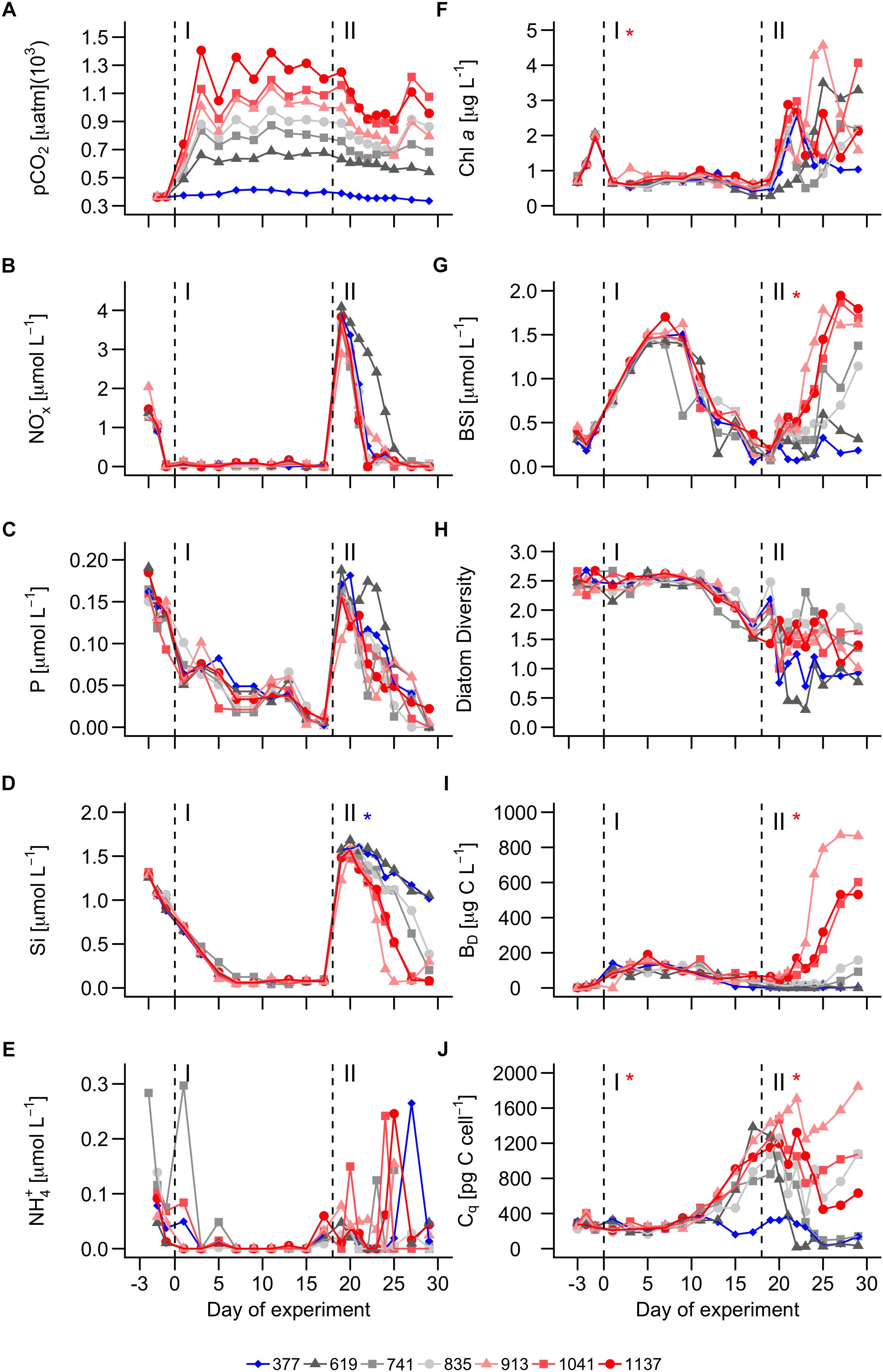
Figure 2. Chemical conditions and bloom formations in the mesocosms. (A) pCO2. (B) Nitrate + Nitrite concentrations. (C) Phosphate concentration. (D) Dissolved silicate concentration. (E) Ammonium concentration. (F) Chlorophyll a concentration. (G) Biogenic silica. (H) Shannon-Weaver diversity of the diatom community. (I) total diatom biomass. (J) Cellular C quota averaged over all diatom species (see Eq. 2). Dashed vertical lines separate the three phases of the experiment. Asterisks indicate significantly (p < 0.05) positive (red) or negative (blue) CO2 effects during phases. The legend at the bottom gives mean pCO2 values (in μatm) of the different treatments.
At the beginning of the study (day -3), nutrient concentrations were 1.46 ± 0.27, 0.17 ± 0.02, 1.29 ± 0.2, 0.47 ± 0.15 μmol L-1 for NOx-, P, Si, and NH4+, respectively. These nutrient concentrations were well within the natural range observed in the surface at the nearby European Station for Time Series in the Ocean at the Canary Islands (ESTOC), located in the NE Atlantic subtropical gyre (Cianca et al., 2007). Nutrient concentrations were declining from day -3 onward but at different rates (NOx- > NH4+ > Si > P; Figure 2). All nutrients were exhausted by the end of phase I and hence before nutrient enrichment on day 18 (Figure 2).
NOx-, P, and Si concentrations were moderately increased on day 18 and averaged at 3.43 ± 0.32, 0.16 ± 0.01, and 1.63 ± 0.12 μmol L-1 directly after the nutrient enrichment. These N:P:Si ratios roughly correspond to those of deep water (∼600 m) around the study area (Taucher et al., 2017). The fertilization induced phytoplankton growth and corresponding nutrient drawdown. NOx- declined fastest reaching values from before the bloom between days 23–25, and on day 27 in the 619 μatm treatment (Figure 2B). P reached pre-bloom values between days 27 and 29, albeit not in the 1137 μatm treatment (Figure 2C). Si reached pre-bloom values between days 25 and 27 in the three highest CO2 treatments, whereas Si remained at significantly (p < 0.05) higher levels in the two lowest CO2 mesocosms until the end of the experiment (>1 μmol L-1; Figure 2D). NH4+ was not added during the nutrient enrichment but concentrations showed a higher day to day variability during phase II (Figure 2E).
Bulk Phytoplankton
Chla concentrations were 0.73 ± 0.07 μmol L-1 on the first sampling day (day -3) and increased quickly to 2 ± 0.04 μmol L-1 on day -1 (Figure 2F), consistent with the decreasing nutrient concentrations (Figures 2B–E). Chla dropped down to the initial values on day 1 and remained quite constant at this level throughout phase I. Chla was slightly, but significantly elevated in the high CO2 treatments during phase I (p = 0.043, Figure 2F). The nutrient enrichment on day 18 led to a rapid chla increase in all mesocosms except for the 619 μatm treatment. Here, the increase was delayed since the chla concentration at the onset of the bloom was considerably lower than in the other mesocosms (check Figure 2F on day 18). CO2 had no significant influence on chla during phase II.
Biogenic silica concentrations were 0.36 ± 0.07 μmol L-1 on the first sampling day (day -3). Concentrations increased thereafter in all mesocosms until peaking at 1.5 ± 0.1 μmol L-1 on day 7. BSi declined after the peak to 0.22 ± 0.11 μmol L-1 at the end of phase I (Figure 2G). CO2 had a significant positive influence on the BSi development after the nutrient fertilization (p = 0.002). BSi increased to values slightly lower than 2 μmol L-1 in the three highest CO2 mesocosms (day 29), while hardly any increase was observed in the two lowest CO2 mesocosms (day 29; Figure 2G). The BSi development over the course of the study is reflected in the development of dissolved Si (compare Figures 2D,G; please note that the BSi decline at the end of phase I is not leading to increasing concentrations of dissolved Si since the BSi sinks out into the sediment traps and is therefore removed from the water columns).
Diatom Communities
The diatom community was initially diverse (Figure 2H) and dominated by species that are frequently found in the region (Anabalón et al., 2014). The genera with highest C biomass contribution in the mesocosms were: Guinardia (Guin), Rhizosolenia (Rhiz), Cerataulina (Cera), Thalassiosira (Thals), Dactyliosolen (Dact), Chaetoceros (Chae), Skeletonema (Skel), Leptocylindrus (Lept), and Pseudo-nitzschia (Ps-n). These are shown on an individual basis in Figures 3, 4. Subdominant species were pooled and shown as one group (“others,” Figures 3, 4). A full species list with calculated biovolumes and C biomasses is provided in Table 1. The PCoA of phase 0 revealed no treatment-specific dissimilarities between mesocosms before the first CO2 addition (Figure 5A). The three highest CO2 treatments were mapped at the extremes of the PCo space. This information is important as it indicates that dissimilarities between treatments later in the experiment are less likely to be predetermined by the initial diatom community structure.
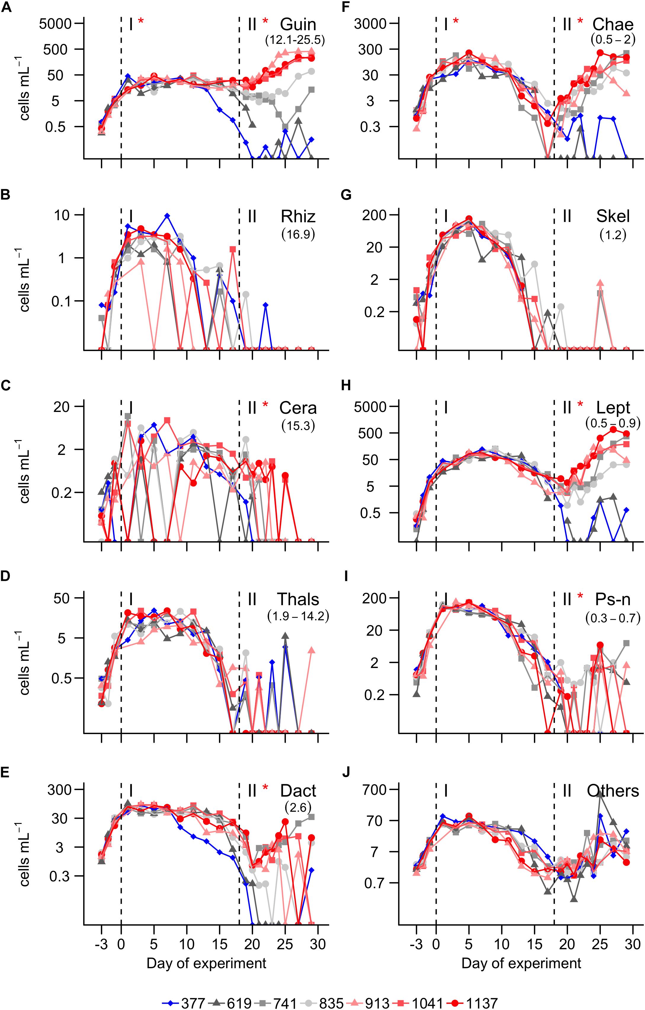
Figure 3. Abundance of the most important diatom genera. (A) Guinardia. (B) Rhizosolenia. (C) Cerataulina. (D) Thalassiosira. (E) Dactyliosolen. (F) Chaetoceros. (G) Skeletonema. (H) Leptocylindrus. (I) Pseudo-nitzschia. (J) Sum of all other diatom species. A full species list is provided in Table 1. Dashed vertical lines separate the three phases of the experiment. Asterisks indicate significantly (p < 0.05) positive (red) or negative (blue) CO2 effects during phases. The legend at the bottom gives mean pCO2 values (in μatm) of the different treatments.
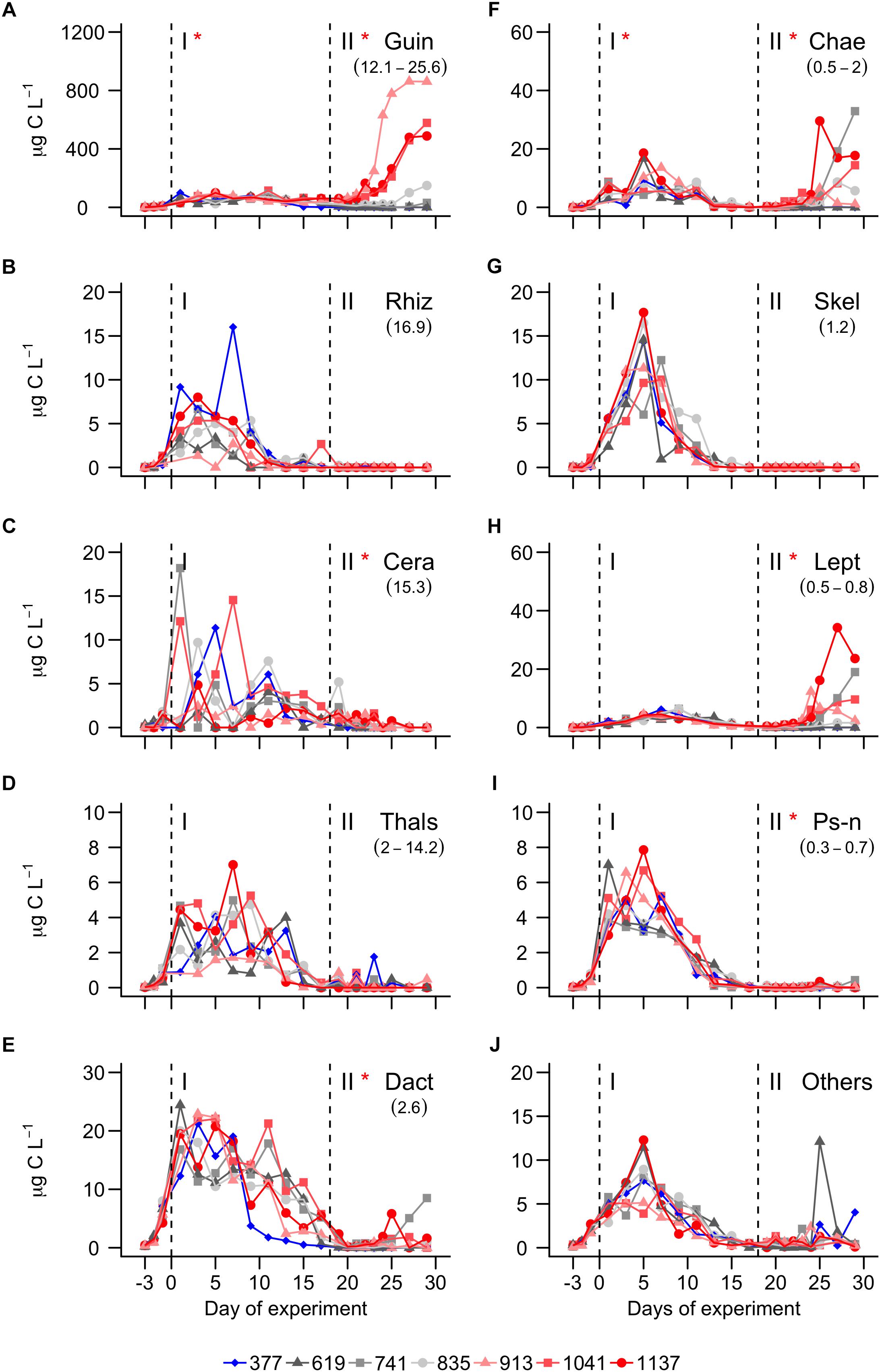
Figure 4. C Biomass of the most important diatom genera. (A) Guinardia. (B) Rhizosolenia. (C) Cerataulina. (D) Thalassiosira. (E) Dactyliosolen. (F) Chaetoceros. (G) Skeletonema. (H) Leptocylindrus. (I) Pseudo-nitzschia. (J) Sum of all other diatom species. A full species list is provided in Table 1. Dashed vertical lines separate the three phases of the experiment. Asterisks indicate significantly (p < 0.05) positive (red) or negative (blue) CO2 effects during phases. The legend at the bottom gives mean pCO2 values (in μatm) of the different treatments.
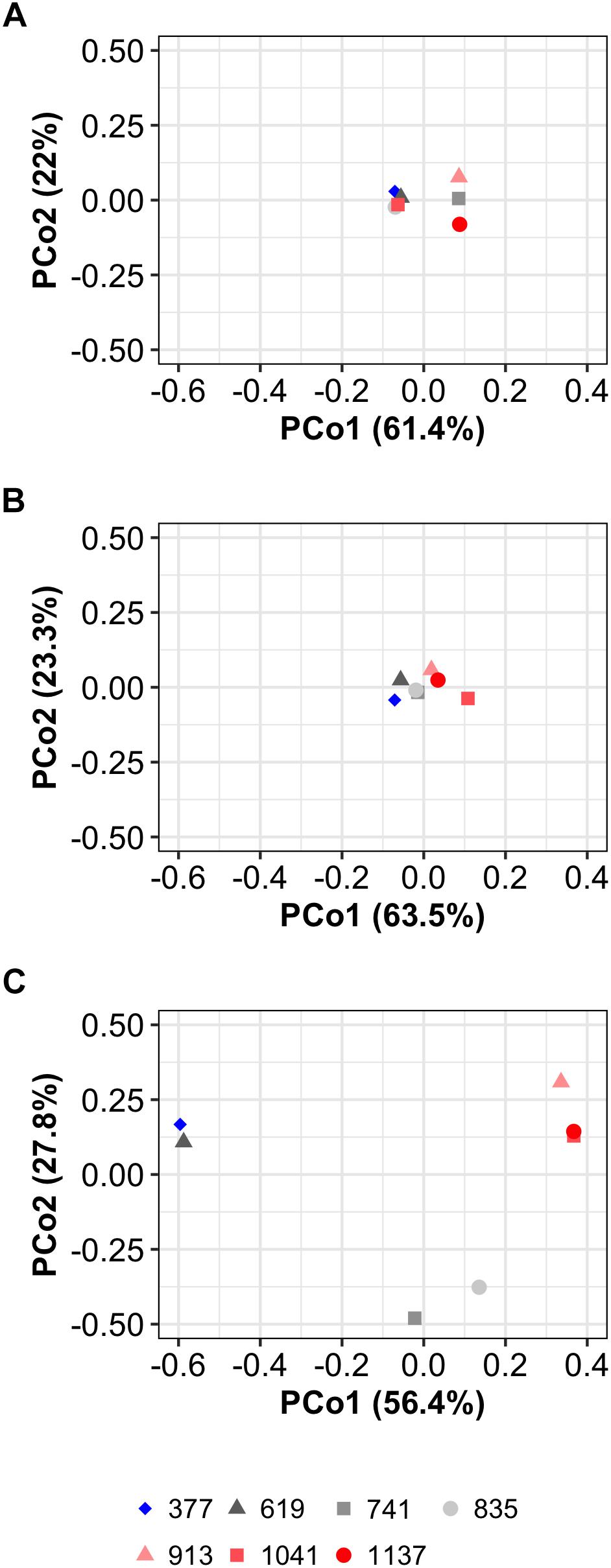
Figure 5. PCoA analyses of the diatom community composition. (A) Phase 0 (i.e., before the CO2 manipulation). (B) Phase I. (C) Phase II. Explained variance for principal coordinates 1 and 2 (PCo1, PCo2) are given on the axis. The legend at the bottom gives mean PCo2 values (in μatm) of the different treatments.
Diatoms started to grow exponentially at the beginning of the study until days 1 to 5, reflected in the BSi build-up and Si drawdown (Figures 2D,G). Abundance and C biomass declined after this initial peak but in some genera (e.g., Skeletonema) more than in others (e.g., Guinardia; compare Figures 3A, 4A with Figures 3G, 4G). The decline of some species to almost undetectable abundances toward the end of phase I led to a decrease of diversity from ∼2 (days -3–13) to ∼1.2 (days 17–29; Figure 2H). Diatoms developed similarly in all treatments during the more oligotrophic conditions in phase I, but we detected significant CO2 effects on abundance and C biomass of Guinardia and Chaetoceros (Figures 3A,F and Table 2). Cq (Eq. 2) of the diatom community averaged over phase I was positively correlated with pCO2 (Figure 2J). The PCoA of phase I revealed no pronounced CO2-dependent dissimilarities of the diatom communities, although there is, perhaps, a mild separation between the three highest CO2 mesocosms and the control along PCo1 (Figure 5B).
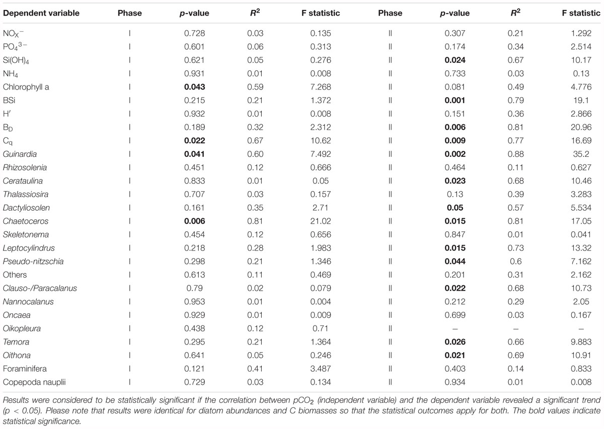
Table 2. Statistics; Regression analyses were performed for time-averaged means for the two experimental phases.
A pronounced diatom bloom was initiated through the nutrient fertilization at the beginning of phase II. However, the onset of the bloom varied among the different diatom genera. While Chaetoceros was responding immediately (day 18), it took most of the other genera a few days before they started to grow (Figure 3B). Nanoflagellates (0.2–2 μm) were profiting from this delay (Filella et al., 2018) and were largely responsible for the first chla peak on day 22, shortly after nutrient fertilization (Figure 2B). Diatoms became more influential on the bulk chla signal about 1 week after fertilization (compare Figures 2B, 4), although other groups like non-diazotrophic cyanobacteria, dinoflagellates, or nanoflagellates still had a noticable influence (Filella et al., 2018).
CO2 had a strong influence on the composition of the diatom assemblage after the nutrient fertilization. Abundance and C biomass of Cerataulina, Chaetoceros, Dactyliosolen, Guinardia, Leptocylindrus, and Pseudo-nitzschia were significantly positively influenced under high CO2. Guinardia was the species with the highest carbon content and profited most strongly from high CO2 levels (Figures 3D, 4D). Cq of the diatom community was positively correlated with pCO2 during phase I and II (Figure 2I, phase I, p = 0.022; phase II p = 0.009). The PCoA for phase II revealed CO2-dependent dissimilarities of the diatom community where the control and the 619 μatm treatment, the 741 and the 835 μatm treatments, and the three highest CO2 treatments were mapped in three different regions of the PCo space (Figure 5C).
Mesozooplankton
The MesoZP communities were numerically dominated by copepods (Figure 6). Individuals of the different species were generally small with even the adults hardly ever being larger than 500 μm. The two genera Clausocalanus and Paracalanus were not distinguishable while counting the sample and were therefore merged into one taxonomic unit, termed CP-calanus in the following (please note that both genera were present in the mesocosms as was determined with meta-barcoding). The most abundant copepod genera during phase I were CP-calanus, Oithona, Oncaea, and Temora (Figures 6A,C,E,F). CP-calanus and Temora reached particularly high abundances during phase II but only in the lower CO2 mesocosms (Figures 6A,E). Copepod nauplii reached abundance peaks on days 13 and 30, although there was a large spread among mesocosms especially during the second peak (Figure 6H). Other MesoZP taxa that occurred in high abundances comprised Oikopleura dioica (appendicularia) and foraminifera (most likely Globigerinidae species). O. dioica was initially not detected but occurred suddenly in some mesocosms during phase I (Figure 6D). It disappeared equally quickly after the bloom and remained detectable only in the 619 and 913 μatm treatments (Figure 6D). Foraminifera were detected in low abundances since the first sampling and they thrived in all mesocosms until day 21–25 (Figure 6G).
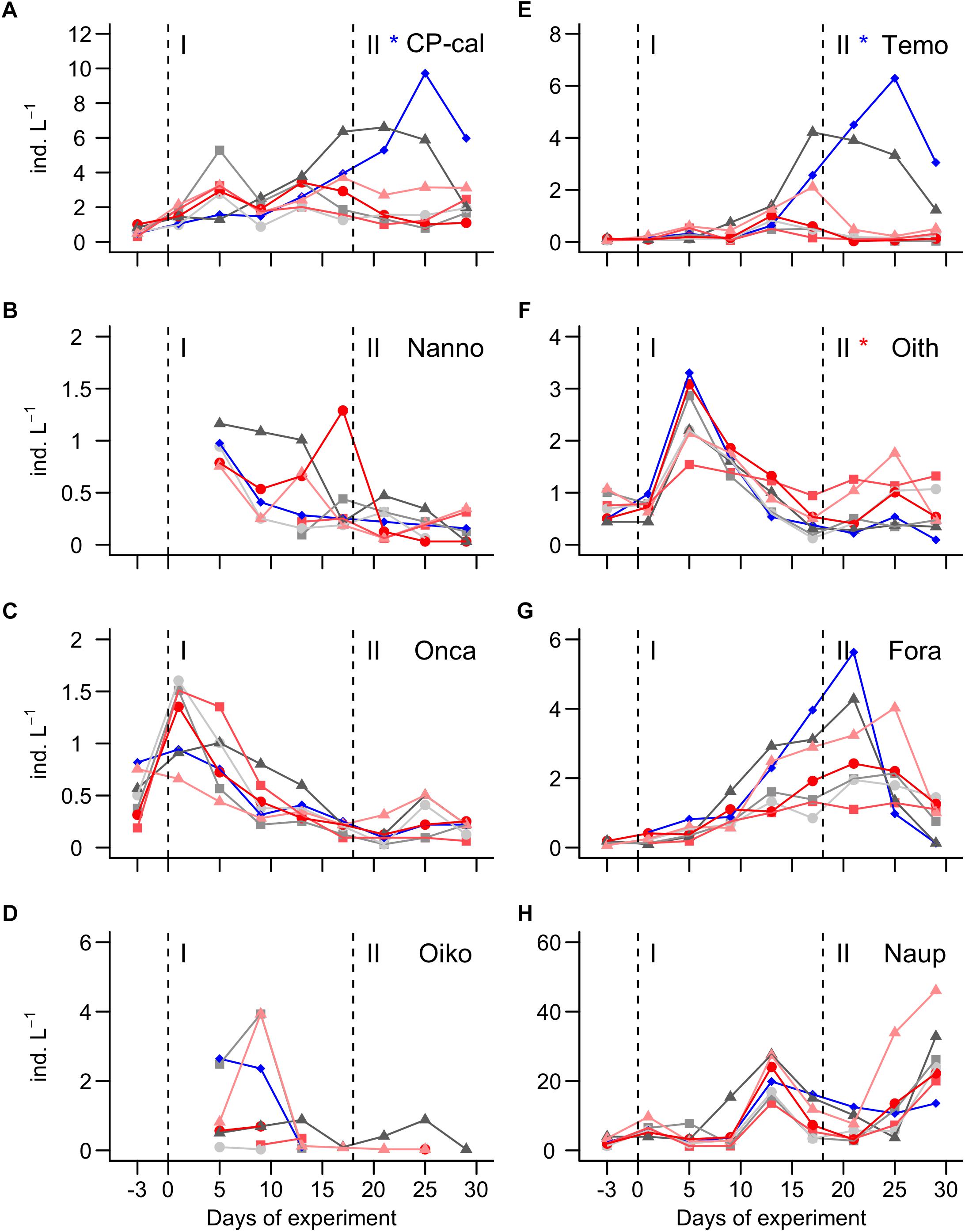
Figure 6. Abundance of the most important mesozooplankton groups (A) CP-calanus. (B) Nannocalanus. (C) Oncaea. (D) Oikopleura dioica. (E) Temora. (F) Oithona. (G) Foraminifera. (H) Nauplii. Dashed vertical lines separate the three phases of the experiment. Asterisks indicate significantly (p < 0.05) positive (red) or negative (blue) CO2 effects during phases. The legend at the bottom gives mean pCO2 values (in μatm) of the different treatments.
CO2 effects on MesoZP were detected only in 3 species and only in phase II. CO2 had a strong positive influence on the abundance of CP-calanus and Temora (Figures 6A,E). Oithona was negatively affected by CO2 but the effect was not as pronounced as in the two other genera (Figure 6F).
Discussion
Physiological studies have shown that growth and the metabolism of diatoms can be affected by increasing seawater CO2 concentrations (Gao and Campbell, 2014). A recent meta-analysis of OA laboratory experiments with diatoms revealed an increase of growth rates under high CO2, although the response varies widely among different diatom species (Dutkiewicz et al., 2015). This inter-specific variability is an important feature as it suggests that high CO2 conditions will affect diatom species differentially and therefore, alter the composure of diatom assemblages (Tortell et al., 2008; Hoppe et al., 2013; Endo et al., 2016). Indeed, our experiment revealed a positive effect on the bulk diatom biomass (Cq) that coincided with shifts in the assemblage structure after the nutrient addition.
The exact mechanisms which control diatom responses to high CO2 are difficult to uncover in mesocosm experiments because the complexity of the food web allows a myriad of explanations (Bach et al., 2017). Therefore, our goal in the discussion is not to mention every imaginable mechanism but to highlight particularly plausible ones while acknowledging that none of them can be proven and none are necessarily exclusive. In fact, several mechanisms could coincide and ultimately explain the observed responses together. After discussing potential mechanisms underlying the observed CO2 responses (section “Potential Mechanisms Explaining Observed CO2 Effects on the Diatoms”), we consider our findings in a wider perspective and discuss their value to assess diatom responses to OA in the subtropical NE Atlantic (section “What Can These Results Tell Us About OA Impacts on Diatoms in the Subtropical NE Atlantic?”).
Potential Mechanisms Explaining Observed CO2 Effects on the Diatoms
CO2 Fertilization of Photosynthesis
When phytoplankton profits from high CO2 then this is usually explained with a CO2 fertilization effect on inorganic carbon acquisition. The idea is that increasing seawater pCO2 facilitates the diffusive uptake of CO2, thereby reducing the energy demand for active carbon acquisition (Giordano et al., 2005; Reinfelder, 2011). The energy that is saved by reducing the operation of this so-called “carbon concentrating mechanism (CCM)” can be diverted into the acquisition of other resources, ultimately leading to faster growth. Physiological studies with diatoms generally support this concept, although variability exists between species (Rost et al., 2003; Hopkinson et al., 2011; Trimborn et al., 2013; Gao and Campbell, 2014).
The CCM related explanation may also apply to our results. Elevated pCO2 may have stimulated resource acquisition in some of the diatom species present in the mesocosms, thereby leading to CO2-dependent restructuring of the assemblage. Recently, Wu et al. (2014) performed laboratory CO2 experiments with four different Thalassiosira species and Coscinodiscus wailesii, and found that the CO2 fertilization effect on growth rates scales positively with cell volume. Although their concept is derived mainly from one genus, it is physiologically well substantiated and based on the positive correlation between cell size and diffusion gradients, which predicts that high CO2 is particularly beneficial for carbon acquisition in larger species (Pasciak and Gavis, 1974; Wolf-Gladrow and Riebesell, 1997; Flynn et al., 2012; Shen and Hopkinson, 2015). Applying the cell volume dependency determined by Wu et al. (2014) to our dataset partially confirms their concept. As predicted, we observed by far the strongest CO2 stimulation in Guinardia, the largest genus present in the experiment. Apart from Guinardia, however, CO2 effects did not seem to scale with diatom biovolumes. There were small genera (e.g., Chaetoceros) that showed clearer CO2 responses than larger ones (e.g., Cerataulina) (Figures 3C,F). Hence, while the Wu et al. (2014) concept provides a great starting point to interpret results observed in field experiments, it still needs to be expanded to account for the ecological complexities occurring outside the laboratory environment and genotype-specific variability. The application of molecular tools in community studies may help to make significant progress on that matter (Endo et al., 2016).
CO2 Effect Through Grazer Interactions
Copepods were the most abundant MesoZP group present in the mesocosms and probably had a top-down impact on the diatom community. Three of the five dominant copepod genera were significantly influenced by high CO2 during phase II. Oithona abundance ranged between 100 and 1800 individuals L-1 and was positively affected (Figure 6F). In contrast, CP-calanus and Temora abundances ranged between 800 to 9700 and 30 to 6900 individuals L-1, respectively, and were both negatively affected by high CO2 (Figures 6A,E). The higher abundances of CP-calanus and Temora, as well as the larger CO2 effect size relative to Oithona, suggests that any CO2-related top-down control was primarily mediated through these two species. Indeed, abundances of several diatom species and bulk diatom biomass were significantly reduced under high CO2 during phase II and particularly low in the control and the lowest CO2 treatment (619 μatm), where considerably more CP-calanus and Temora were present (compare Figures 2I, 6A,E). This anti-correlated pattern points toward a causal relationship between diatom and CP-calanus/Temora abundances that were altered through CO2 concentrations. The key question is: Through which mechanisms could CO2 affect the interaction between copepods and diatoms?
The most straight-forward explanation would be a negative CO2 effect on the physiological performance of CP-calanus and Temora. High CO2/low pH conditions may have reduced growth and grazing of these two copepod genera, thereby reducing their abundances and ultimately grazing pressure on diatoms. To the best of our knowledge, there is no published study to date in which direct CO2 effects on CP-calanus were investigated under controlled laboratory conditions. Such experiments exist for Temora longicornis but it is unclear whether the Temora species in our experiments would show the same insensitivity to high CO2 as the individuals from the English Channel investigated by McConville et al. (2013). Recent OA experiments with Calanus glacialis revealed population-specific CO2 responses with more robust populations found in naturally CO2-rich habitats (Thor et al., 2018). These findings suggest that local carbonate chemistry conditions may be a better predictor to assess CO2 sensitivities of copepods than their taxonomic affiliation (Thor et al., 2018; Zhang et al., 2018). They also suggest that laboratory-based results can only reliably be used to interpret responses observed in experiments with natural assemblages when both experiments were done with individuals from the same population. Thus, with the available data it is not possible to assess the likelihood for such a direct negative CO2 effect on the metabolism of CP-calanus and Temora.
Altered interactions between CP-calanus/Temora and diatoms could also have been provoked through CO2-induced changes in the nutritional quality of the diatoms. If high CO2 triggers a physiological response in diatoms, that cause them to be less nutritious, copepod growth would be reduced ultimately leading to lower grazing pressure and higher diatom abundances. A potential explanation for this hypothesis comes from experiments by Rossoll et al. (2012), who found that the diatom Thalassiosira pseudonana contained less fatty acids under high CO2 and the composition of the produced fatty acids had a lower nutritional value. As a consequence, the copepod Acartia tonsa fed with these T. pseudonana cells grew slower and produced less eggs (Rossoll et al., 2012). Furthermore, carbonate chemistry effects on silicification may have altered the strength of the frustule and therefore the palatability of diatoms (Hamm et al., 2003; Wilken et al., 2011; Friedrichs et al., 2013; Liu et al., 2016). Low seawater pH is considered to be beneficial for the silicification process since opal precipitation does occur in a low pH (pH ∼5) compartment of the diatom cell (Vrieling et al., 1999; Martin-Jézéquel et al., 2000). Indeed, Hervé et al. (2012) found increasing Si incorporation and cellular BSi quota in T. weissflogii with decreasing pH from 8 to 7.2. However, other experiments with T. weissflogii only found increased Si uptake rates (Milligan et al., 2004) but decreasing BSi quota (Milligan et al., 2004) or BSi/C (Mejía et al., 2013). Thus, with the currently available (and partially controversial) information, it is not possible to assess the relevance of carbonate chemistry dependent silicification changes on grazing but it would be worthwhile to further investigate this important feedback in future studies (Milligan et al., 2004; Mejía et al., 2013; Gao and Campbell, 2014).
What Can These Results Tell Us About OA Impacts on Diatoms in the Subtropical NE Atlantic?
The potential of OA impacts on diatom communities will depend on the degree of future CO2 increase. In the present experiment, diatom composition was noticeably affected at pCO2 levels >619 μatm, during the bloom in phase II (Figure 5C). This should not be regarded as a general threshold for diatom OA sensitivity as it is likely to vary regionally, depending on the prevailing diatom community and regional carbonate chemistry conditions. More productive regions near coasts or estuaries have typically larger natural variations in carbonate chemistry (Hofmann et al., 2011; Wallace et al., 2014) and should harbor generalist species, which are less responsive to increased CO2. Conversely, CO2 enrichment studies in more stable oceanic environments should be more likely to induce a response (Duarte et al., 2013). Carbonate chemistry conditions at the coast of Gran Canaria are rather stable with comparatively little seasonal fluctuations (González-Dávila et al., 2010), which may explain why quite pronounced changes in the diatom community composition were observed already above 619 μatm.
The experiment discussed in the present paper took place in spring 2016 but we did a similar OA experiment at the coast of Gran Canaria with larger mesocosms already in autumn 2014 (Taucher et al., 2017). In this earlier experiment we also observed profound shifts in the diatom community composition, although the CO2 threshold above which changes occurred could not be determined (Taucher et al., 2018). The diatom genera Guinardia and Leptocylindrus were important in both the 2016 and the 2014 study and the comparison of their responses to high CO2 is valuable because it allows us to assess the “reproducibility” of our findings. Guinardia benefitted profoundly from high CO2 in both experiments which raises confidence that the Guinardia species enclosed in the mesocosms (G. striata in 2014; G. delicatula, Guinardia spp. in 2016) could become more competitive in an acidified NE Atlantic. Leptocylindrus, however, responded oppositely which could be due to different Leptocylindrus genotypes being enclosed in the mesocosms (L. delicatulum in 2014; Leptocylindrus spp. in 2016). Alternatively, different food web structures could have indirectly caused the opposite responses, for example by altering resource competition or grazing pressure. Such food web related differences could have either developed in the course of the study or were already established at the beginning when the communities were enclosed inside the mesocosms (Moreno de Castro et al., 2017). In this context it is also important remember that the mesocosm bags were filled with pumps in 2016 (section “Mesocosm Design, Deployment, and Maintenance”) while they were lowered into the water column in 2014 (Taucher et al., 2017). The different filling procedures may have amplified differences in the initial community structure.
The Guinardia species enclosed in the mesocosms was a comparatively large diatom and its positive response to high CO2 drove the significant increase of the average cellular carbon quota (Cq) of the diatom community (Figure 2J). Such a CO2-induced shift toward larger diatoms was also observed in several earlier OA experiments with natural communities (Tortell et al., 2008; Feng et al., 2009, 2010; Eggers et al., 2014; Bach et al., 2017; Taucher et al., 2018) while the opposite response (i.e., a CO2-induced shift toward smaller diatoms) was reported only once (Davidson et al., 2016). This suggests that OA will generally favor large diatom species, which is in accordance with the physiological theory described at the beginning of section “Potential Mechanisms Explaining Observed CO2 Effects on the Diatoms”.
Conclusion
In this study we enclosed a natural plankton community from the subtropical NE Atlantic in in situ mesocosms to assess their response to simulated future ocean acidification. Our findings suggest that the bulk diatom community in the subtropical NE Atlantic could benefit from high CO2 conditions projected for the end of this century under nutrient supply (e.g., via seasonal or eddy-induced upwelling). However, the positive CO2 response of the bulk diatom biomass coincided with pronounced shifts in the diatom species composition because not all diatoms benefitted equally from high CO2. The largest diatom genus in the mesocosms (Guinardia) was particularly CO2 responsive and its pronounced dominance under high CO2 caused a significant increase in the average size of the diatom community. The particularly strong CO2 effect on a large diatom is in accordance with physiological theory and has been observed in earlier studies, which adds confidence to this finding. Nevertheless, the discussed example of the response of Leptocylindrus to high CO2 revealed that many uncertainties are yet to be resolved before winners and losers within the diatom community can be determined with high confidence.
Data Availability
The datasets generated for this study are available on request to the corresponding author.
Author Contributions
LB, JT, UR, and JA designed the experiments. All authors conducted the experiments. LB, NH-H, JT, CaS, and ClS measured the data. LB and NH-H analyzed the data. NH-H performed the statistical analysis and plotted the data. LB drafted the manuscript. LB, NH-H, JT, CaS, UR, and JA revised the manuscript.
Funding
This study was financially supported by Cluster of Excellence “The Future Ocean” at the University of Kiel. JA was supported by a Helmholtz International Fellow Award, 2015 (Helmholtz Association, Germany). NH-H and JA benefited also from the FLUXES project (CTM2015-69392-C3-1-R) funded by the Spanish government (Plan Nacional I+D).
Conflict of Interest Statement
The authors declare that the research was conducted in the absence of any commercial or financial relationships that could be construed as a potential conflict of interest.
Acknowledgments
We thank Shaomin Chen, Syrmalenia Kotronaki, Peter Fritzsche, Andrea Ludwig, Jana Meyer, Alice Nauendorf, and Lena Soumpasis for measuring carbonate chemistry, nutrient, and BSi samples, Andrea Ludwig for logistical support and CTD operations, Michael Krudewig, Michael Sswat, Peter Kohnert, Mario Deckelnick, and Jan Czerny for construction of the mesocosm infrastructure. Furthermore, we also thank the Oceanic Platform of the Canary Islands (PLOCAN) and its staff for the use of their facilities, and for their help with the logistics and organization of this experiment.
Footnotes
References
Anabalón, V., Arístegui, J., Morales, C. E., Andrade, I., Benavides, M., Correa-Ramírez, M. A., et al. (2014). The structure of planktonic communities under variable coastal upwelling conditions off Cape Ghir (31°N) in the Canary Current System (NW Africa). Prog. Oceanogr. 120, 320–339. doi: 10.1016/j.pocean.2013.10.015
Arístegui, J., Barton, E. D., Tett, P., Montero, M. F., García-Muñoz, M., Basterretxea, G., et al. (2004). Variability in plankton community structure, metabolism, and vertical carbon fluxes along an upwelling filament (Cape Juby, NW Africa). Prog. Oceanogr. 62, 95–113. doi: 10.1016/j.pocean.2004.07.004
Armbrust, E. V. (2009). The life of diatoms in the world’s oceans. Nature 459, 185–192. doi: 10.1038/nature08057
Bach, L. T., Alvarez-Fernandez, S., Hornick, T., Stuhr, A., and Riebesell, U. (2017). Simulated ocean acidification reveals winners and losers in coastal phytoplankton. PLoS One 12:e0188198. doi: 10.1371/journal.pone.0188198
Bach, L. T., Taucher, J., Boxhammer, T., Ludwig, A., Achterberg, E. P., Algueró-Muñiz, M., et al. (2016). Influence of ocean acidification on a natural winter-to-summer plankton succession: first insights from a long-term mesocosm study draw attention to periods of low nutrient concentrations. PLoS One 11:e0159068. doi: 10.1371/journal.pone.0159068
Barton, E. D., Aristegui, J., Tett, P., Canton, M., García-Braun, J., Hernández-León, S., et al. (1998). The transition zone of the Canary Current upwelling region. Prog. Oceanogr. 41, 455–504. doi: 10.1016/S0079-6611(98)00023-8
Boxhammer, T., Bach, L. T., Czerny, J., and Riebesell, U. (2016). Technical note: sampling and processing of mesocosm sediment trap material for quantitative biogeochemical analysis. Biogeosciences 13, 2849–2858. doi: 10.5194/bg-13-2849-2016
Boyd, P., and Newton, P. (1995). Evidence of the potential influence of planktonic community structure on the interannual variability of particulate organic carbon flux. Deep Sea Res. Part I Oceanogr. Res. Pap. 42, 619–639. doi: 10.1016/0967-0637(95)00017-Z
Brzezinski, M. A., and Nelson, D. M. (1996). Chronic substrate limitation of silicic acid uptake rates in the western Sargasso Sea. Deep Sea Res. Part II Top. Stud. Oceanogr. 43, 437–453. doi: 10.1016/0967-0645(95)00099-2
Cianca, A., Helmke, P., Mouriño, B., Rueda, M. J., Llinás, O., and Neuer, S. (2007). Decadal analysis of hydrography and in situ nutrient budgets in the western and eastern North Atlantic subtropical gyre. J. Geophys. Res. Ocean. 112:C07025. doi: 10.1029/2006JC003788
Davidson, A., McKinlay, J., Westwood, K., Thomson, P., van den Enden, R., de Salas, M., et al. (2016). Enhanced CO2 concentrations change the structure of Antarctic marine microbial communities. Mar. Ecol. Prog. Ser. 552, 93–113. doi: 10.3354/meps11742
Dickson, A. G., Afghan, J. D., and Anderson, G. C. (2003). Reference materials for oceanic CO2 analysis: a method for the certification of total alkalinity. Mar. Chem. 80, 185–197. doi: 10.1016/S0304-4203(02)00133-0
Dickson, A. G., Sabine, C. L., and Christian, J. R. (2007). Guide to Best Practices for Ocean CO2 Measurements. Sidney: North Pacific Marine Science Organization.
Duarte, C. M., Hendriks, I. E., Moore, T. S., Olsen, Y. S., Steckbauer, A., Ramajo, L., et al. (2013). Is ocean acidification an open-ocean syndrome? understanding anthropogenic impacts on seawater pH. Estuaries and Coasts 36, 221–236. doi: 10.1007/s12237-013-9594-3
Dutkiewicz, S., Morris, J. J., Follows, M. J., Scott, J., Levitan, O., Dyhrman, S. T., et al. (2015). Impact of ocean acidification on the structure of future phytoplankton communities. Nat. Clim. Chang. 5, 1002–1006. doi: 10.1038/nclimate2722
Eggers, S. L., Lewandowska, A. M., Barcelos E Ramos, J., Blanco-Ameijeiras, S., Gallo, F., and Matthiessen, B. (2014). Community composition has greater impact on the functioning of marine phytoplankton communities than ocean acidification. Glob. Chang. Biol 20, 713–723. doi: 10.1111/gcb.12421
Endo, H., Sugie, K., Yoshimura, T., and Suzuki, K. (2016). Response of Spring Diatoms to CO2 Availability in the Western North Pacific as Determined by Next-Generation Sequencing. PLoS One 11:e0154291. doi: 10.1371/journal.pone.0154291
Feng, Y., Hare, C. E., Leblanc, K., Rose, J. M., Zhang, Y., DiTullio, G. R., et al. (2009). Effects of increased pCO2 and temperature on the north atlantic spring bloom. I. The phytoplankton community and biogeochemical response. Mar. Ecol. Prog. Ser. 388, 13–25. doi: 10.3354/meps08133
Feng, Y., Hare, C. E., Rose, J. M., Handy, S. M., DiTullio, G. R., Lee, P. A., et al. (2010). Interactive effects of iron, irradiance and CO2 on Ross Sea phytoplankton. Deep. Res. Part I Oceanogr. Res. Pap. 57, 368–383. doi: 10.1016/j.dsr.2009.10.013
Field, C. B., Behrenfeld, M. J., Randerson, J. T., and Falkowski, P. G. (1998). Primary Production of the Biosphere: Integrating Terrestrial and Oceanic Components. Science 281, 237–240. doi: 10.1126/science.281.5374.237
Filella, A., Baños, I., Montero, M. F., Hernández-Hernández, N., Rodriguez-Santos, A., Ludwig, A., et al. (2018). Plankton Community Respiration and ETS Activity Under Variable CO2 and Nutrient Fertilization During a Mesocosm Study in the Subtropical North Atlantic. Front. Mar. Sci. 5:310. doi: 10.3389/fmars.2018.00310
Flynn, K. J., Blackford, J. C., Baird, M. E., Raven, J. A., Clark, D. R., Beardall, J., et al. (2012). Changes in pH at the exterior surface of plankton with ocean acidification. Nat. Clim. Chang. 2, 510–513. doi: 10.1038/nclimate1489
Friedrichs, L., Hörnig, M., Schulze, L., Bertram, A., Jansen, S., and Hamm, C. (2013). Size and biomechanic properties of diatom frustules influence food uptake by copepods. Mar. Ecol. Prog. Ser. 481, 41–51. doi: 10.3354/meps10227
Gao, K., and Campbell, D. A. (2014). Photophysiological responses of marine diatoms to elevated CO2 and decreased pH: A review. Funct. Plant Biol. 41, 449–459. doi: 10.1071/FP13247
Giordano, M., Beardall, J., and Raven, J. A. (2005). CO2 concentrating mechanisms in algae: mechanisms, environmental modulation, and evolution. Annu. Rev. Plant Biol. 56, 99–131. doi: 10.1146/annurev.arplant.56.032604.144052
González-Dávila, M., Santana-Casiano, J. M., Rueda, M. J., and Llinás, O. (2010). The water column distribution of carbonate system variables at the ESTOC site from 1995 to 2004. Biogeosciences 7, 3067–3081. doi: 10.5194/bg-7-3067-2010
Hamm, C., and Smetacek, V. (2007). “Armor: Why, when, and how,” in Evolution of Phytoplankton, eds P. G. Falkowski and A. H. Knoll (Boston, MA: Elsevier), 311–332.
Hamm, C. E., Merkel, R., Springer, O., Jurkojc, P., Maiert, C., Prechtelt, K., et al. (2003). Architecture and material properties of diatom shells provide effective mechanical protection. Nature 421, 841–843. doi: 10.1038/nature01416
Hansen, H. P., and Koroleff, F. (1999). “Determination of nutrients,” in Methods of Seawater Analysis, eds K. Grasshoff, K. Kremling, and M. Ehrhardt (Weinheim: Wiley-VCH), 159–226. doi: 10.1002/9783527613984.ch10
Hervé, V., Derr, J., Douady, S., Quinet, M., Moisan, L., and Lopez, P. J. (2012). Multiparametric Analyses Reveal the pH-Dependence of Silicon Biomineralization in Diatoms. PLoS One 7:e46722. doi: 10.1371/journal.pone.0046722
Hofmann, G. E., Smith, J. E., Johnson, K. S., Send, U., Levin, L. A., Micheli, F., et al. (2011). High-frequency dynamics of ocean pH: A multi-ecosystem comparison. PLoS One 6:e28983. doi: 10.1371/journal.pone.0028983
Holmes, R. M., Aminot, A., Kérouel, R., Hooker, B. A., and Peterson, B. J. (1999). A simple and precise method for measuring ammonium in marine and freshwater ecosystems. Can. J. Fish. Aquat. Sci. 56, 1801–1808. doi: 10.1139/f99-128
Hopkinson, B. M., Dupont, C. L., Allen, A. E., and Morel, F. M. M. (2011). Efficiency of the CO2-concentrating mechanism of diatoms. Proc. Natl. Acad. Sci. U. S. A. 108, 3830–3837. doi: 10.1073/pnas.1018062108
Hoppe, C. J. M., Hassler, C. S., Payne, C. D., Tortell, P. D., Rost, B. R., and Trimborn, S. (2013). Iron limitation modulates ocean acidification effects on Southern Ocean phytoplankton communities. PLoS One 8:e79890. doi: 10.1371/journal.pone.0079890
Lavigne, H., Epitalon, J.-M., and Gattuso, J.-P. (2011). Seacarb: seawater carbonate chemistry with R. R package version 3.0. Available at: http://cran.r-project.org/package=seacarb
Liu, H., Chen, M., Zhu, F., and Harrison, P. J. (2016). Effect of diatom silica content on copepod grazing, growth and reproduction. Front. Mar. Sci. 3:89. doi: 10.3389/fmars.2016.00089
Lueker, T. J., Dickson, A. G., and Keeling, C. D. (2000). Ocean pCO2 calculated from dissolved inorganic carbon, alkalinity, and equations for K1 and K2: Validation based on laboratory measurements of CO2 in gas and seawater at equilibrium. Mar. Chem. 70, 105–119. doi: 10.1016/S0304-4203(00)00022-0
Mann, D. G., and Vanormelingen, P. (2013). An Inordinate Fondness? The Number, Distributions, and Origins of Diatom Species. J. Eukaryot. Microbiol. 60, 414–420. doi: 10.1111/jeu.12047
Martin-Jézéquel, V., Hildebrand, M., and Brzezinski, M. A. (2000). Review Silicon Metabolism in Diatoms: Implications for Growth. J. Phycol. 36, 821–840. doi: 10.1046/j.1529-8817.2000.00019.x
McConville, K., Halsband, C., Fileman, E. S., Somerfield, P. J., Findlay, H. S., and Spicer, J. I. (2013). Effects of elevated CO2on the reproduction of two calanoid copepods. Mar. Pollut. Bull. 73, 428–434. doi: 10.1016/j.marpolbul.2013.02.010
McGillicuddy, D. J., Anderson, L. A., Bates, N. R., Bibby, T., Buesseler, K. O., Carlson, C. A., et al. (2007). Eddy/Wind Interactions Stimulate Extraordinary Mid-Ocean Plankton Blooms. Science 316, 1021–1026. doi: 10.1126/science.1136256
Mejía, L. M., Isensee, K., Méndez-Vicente, A., Pisonero, J., Shimizu, N., González, C., et al. (2013). B content and Si/C ratios from cultured diatoms (Thalassiosira pseudonana and Thalassiosira weissflogii): Relationship to seawater pH and diatom carbon acquisition. Geochim. Cosmochim. Acta 123, 322–337. doi: 10.1016/j.gca.2013.06.011
Menden-Deuer, S., and Lessard, E. J. (2000). Carbon to volume relationships for dinoflagellates, diatoms, and other protist plankton. Limnol. Oceanogr. 45, 569–579. doi: 10.4319/lo.2000.45.3.0569
Milligan, A. J., Varela, D. E., Brzezinski, M. A., and Morel, F. M. M. (2004). Dynamics of Silicon Metabolism and Silicon Isotopic Discrimination in a Marine Diatom as a Function of pCO2. Limnol. Oceanogr. 49, 322–329. doi: 10.4319/lo.2004.49.2.0322
Moreno de Castro, M., Schartau, M., and Wirtz, K. (2017). Potential sources of variability in mesocosm experiments on the response of phytoplankton to ocean acidification. Biogeosciences 14, 1883–1901. doi: 10.5194/bg-14-1883-2017
Nelson, D. M., Tréguer, P., Brzezinski, M. A., Leynaert, A., and Quéguiner, B. (1995). Production and dissolution of biogenic silica in the ocean: Revised global estimates, comparison with regional data and relationship to biogenic sedimentation. Global Biogeochem. Cycles 9, 359–372. doi: 10.1029/95GB01070
Oksanen, A. J., Blanchet, F. G., Friendly, M., Kindt, R., Legendre, P., Mcglinn, D., et al. (2018). Package “ vegan.” version 2.5-3.
Olenina, I., Hajdu, S., Edler, L., Wasmund, N., Busch, S., Göbel, J., et al. (2006). Biovolumes and size-classes of phytoplankton in the Baltic Sea. HELCOM Balt.Sea Environ. Proc. 106, 144.
Pasciak, W. J., and Gavis, J. (1974). Transport limitation of nutrient uptake in phytoplankton. Limnol. Oceanogr. 19, 881–888. doi: 10.1016/j.cub.2014.12.004
Paul, A. J., Bach, L. T., Schulz, K.-G., Boxhammer, T., Czerny, J., Achterberg, E. P., et al. (2015). Effect of elevated CO2 on organic matter pools and fluxes in a summer Baltic Sea plankton community. Biogeosciences 12, 6181–6203. doi: 10.5194/bg-12-6181-2015
Pondaven, P., Gallinari, M., Chollet, S., Bucciarelli, E., Sarthou, G., Schultes, S., et al. (2007). Grazing-induced Changes in Cell Wall Silicification in a Marine Diatom. Protist 158, 21–28. doi: 10.1016/j.protis.2006.09.002
Reinfelder, J. R. (2011). Carbon concentrating mechanisms in eukaryotic marine phytoplankton. Ann. Rev. Mar. Sci. 3, 291–315. doi: 10.1146/annurev-marine-120709-142720
Riebesell, U., Czerny, J., von Bröckel, K., Boxhammer, T., Büdenbender, J., Deckelnick, M., et al. (2013). Technical Note: A mobile sea-going mesocosm system – new opportunities for ocean change research. Biogeosciences 10, 1835–1847. doi: 10.5194/bg-10-1835-2013
Rossoll, D., Bermúdez, R., Hauss, H., Schulz, K. G., Riebesell, U., Sommer, U., et al. (2012). Ocean acidification-induced food quality deterioration constrains trophic transfer. PLoS One 7:e34737. doi: 10.1371/journal.pone.0034737
Rost, B., Riebesell, U., Burkhardt, S., and Sültemeyer, D. (2003). Carbon acquisition of bloom-forming marine phytoplankton. Limnol. Oceanogr. 48, 55–67. doi: 10.4319/lo.2003.48.1.0055
Sarthou, G., Timmermans, K. R., Blain, S., and Tréguer, P. (2005). Growth physiology and fate of diatoms in the ocean: A review. J. Sea Res. 53, 25–42. doi: 10.1016/j.seares.2004.01.007
Schulz, K. G., Bellerby, R. G. J., Brussaard, C. P. D., Büdenbender, J., Czerny, J., Engel, A., et al. (2013). Temporal biomass dynamics of an Arctic plankton bloom in response to increasing levels of atmospheric carbon dioxide. Biogeosciences 10, 161–180. doi: 10.5194/bg-10-161-2013
Shen, C., and Hopkinson, B. M. (2015). Size scaling of extracellular carbonic anhydrase activity in centric marine diatoms. J. Phycol. 51, 255–263. doi: 10.1111/jpy.12269
Sommer, U., Stibor, H., Katechakis, A., Sommer, F., and Hansen, T. (2002). Pelagic food web confgurations at different levels of nutrient richness and their implications for the ratio fish production:primary production. Hydrobiologia 484, 11–20. doi: 10.1023/A:1021340601986
Strickland, J. D. H., and Parsons, T. R. (1972). in A practical handbook of seawater analysis, ed. J. C. Stevenson Ottawa (Ottawa: Fisheries research board of Canada).
Taucher, J., Arístegui, J., Bach, L. T., Guan, W., Montero, M. F., Nauendorf, A., et al. (2018). Response of Subtropical Phytoplankton Communities to Ocean Acidification Under Oligotrophic Conditions and During Nutrient Fertilization. Front. Mar. Sci. 5:330. doi: 10.3389/fmars.2018.00330
Taucher, J., Bach, L. T., Boxhammer, T., Nauendorf, A., Achterberg, E. P., Algueró-Muñiz, M., et al. (2017). Influence of Ocean Acidification and Deep Water Upwelling on Oligotrophic Plankton Communities in the Subtropical North Atlantic: Insights from an In situ Mesocosm Study. Front. Mar. Sci. 4:85. doi: 10.3389/fmars.2017.00085
Thor, P., Bailey, A., Dupont, S., Calosi, P., Søreide, J. E., De Wit, P., et al. (2018). Contrasting physiological responses to future ocean acidification among Arctic copepod populations. Glob. Chang. Biol. 24, e365–e377. doi: 10.1111/gcb.13870
Tortell, P. D., Payne, C. D., Li, Y., Trimborn, S., Rost, B., Smith, W. O., et al. (2008). CO2 sensitivity of Southern Ocean phytoplankton. Geophys. Res. Lett. 35, L04605. doi: 10.1029/2007GL032583
Tréguer, P., Bowler, C., Moriceau, B., Dutkiewicz, S., Gehlen, M., Aumont, O., et al. (2018). Influence of diatom diversity on the ocean biological carbon pump. Nat. Geosci. 11, 27–37. doi: 10.1038/s41561-017-0028-x
Tréguer, P. J., and De La Rocha, C. L. (2013). The World Ocean Silica Cycle. Ann. Rev. Mar. Sci. 5, 477–501. doi: 10.1146/annurev-marine-121211-172346
Trimborn, S., Brenneis, T., Sweet, E., and Rost, B. (2013). Sensitivity of Antarctic phytoplankton species to ocean acidification: growth, carbon acquisition, and species interaction. Limnol. Oceanogr. 58, 997–1007. doi: 10.4319/lo.2013.58.3.0997
Vrieling, E. G., Gieskes, W. W. C., and Beelen, T. P. M. (1999). Silicon deposition in diatoms: control by the pH inside the silicon deposition vesicle. J. Phycol. 35, 548–559. doi: 10.1046/j.1529-8817.1999.3530548.x
Wallace, R. B., Baumann, H., Grear, J. S., Aller, R. C., and Gobler, C. J. (2014). Coastal ocean acidification: The other eutrophication problem. Estuar. Coast. Shelf Sci. 148, 1–13. doi: 10.1016/j.ecss.2014.05.027
Welschmeyer, N. (1994). Fluorometric analysis of chlorophyll a in the presence of chlorophyll b and pheopigments. Limnol. Oceanogr. 39, 1985–1992. doi: 10.4319/lo.1994.39.8.1985
Wilken, S., Hoffmann, B., Hersch, N., Kirchgessner, N., Dieluweit, S., Rubner, W., et al. (2011). Diatom frustules show increased mechanical strength and altered valve morphology under iron limitation. Limnol. Oceanogr. 56, 1399–1410. doi: 10.4319/lo.2011.56.4.1399
Wolf-Gladrow, D., and Riebesell, U. (1997). Diffusion and reactions in the vicinity of plankton: A refined model for inorganic carbon transport. Mar. Chem. 59, 17–34. doi: 10.1016/S0304-4203(97)00069-8
Wu, Y., Campbell, D. A., Irwin, A. J., Suggett, D. J., and Finkel, Z. V. (2014). Ocean acidification enhances the growth rate of larger diatoms. Limnol. Oceanogr. 59, 1027–1034. doi: 10.4319/lo.2014.59.3.1027
Keywords: ocean acidification, climate change, mesocosm, food web, phytoplankton, Bacillariophyceae
Citation: Bach LT, Hernández-Hernández N, Taucher J, Spisla C, Sforna C, Riebesell U and Arístegui J (2019) Effects of Elevated CO2 on a Natural Diatom Community in the Subtropical NE Atlantic. Front. Mar. Sci. 6:75. doi: 10.3389/fmars.2019.00075
Received: 31 October 2018; Accepted: 11 February 2019;
Published: 01 March 2019.
Edited by:
Laura Anne Bristow, University of Southern Denmark, DenmarkReviewed by:
Koji Suzuki, Hokkaido University, JapanAlex J. Poulton, The Lyell Centre, United Kingdom
Copyright © 2019 Bach, Hernández-Hernández, Taucher, Spisla, Sforna, Riebesell and Arístegui. This is an open-access article distributed under the terms of the Creative Commons Attribution License (CC BY). The use, distribution or reproduction in other forums is permitted, provided the original author(s) and the copyright owner(s) are credited and that the original publication in this journal is cited, in accordance with accepted academic practice. No use, distribution or reproduction is permitted which does not comply with these terms.
*Correspondence: Lennart T. Bach, bGJhY2hAZ2VvbWFyLmRl