 Mats Westerbom
 Olli Mustonen
 Kim Jaatinen
 Mikael Kilpi
 Alf Norkko
- 1Tvärminne Zoological Station, Helsinki University, Helsinki, Finland
- 2Nature and Game Management Trust Finland, Ingå, Finland
- 3Baltic Sea Centre, Stockholm University, Stockholm, Sweden
Examining changes in abundance and demographic rates at species distribution margins may provide the first signs of broader species responses to environmental change. Still, the joint impact of space and time have remained relatively unstudied in most marginal regions. In order to examine the influence of climate variability on mussel distribution patterns, we monitored three sublittoral and marginal blue mussel (Mytilus trossulus) populations, spaced along a salinity gradient. Densities and biomasses peaked toward the saltier parts of the study area and showed relatively larger variations toward the low saline edge. Temporally, the areas showed a consistent increase in abundance after a synchronized large-scale recruitment event, which was followed by a decline in population size, occurring much faster toward the very range edge. Salinity, temperature, winter severity, and wave exposure explained most of the spatiotemporal variation in mussel abundances and adults showed positive effects on recruit abundance. We show empirically that the dynamics of edge populations are not driven by large changes in climate variables but that small spatial and temporal changes in key environmental variables have large and non-linear population level effects. Our results also show that fluctuating recruitment is a key factor for population stability affecting the storage potential of marginal populations, which dramatically decrease toward the edge. Our study provides a window into future population patterns and processes that drive marginal mussel populations in an altered sea characterized by rising temperature and declining salinity.
Introduction
The distribution of many species across the globe is shifting in response to global climate change (e.g., Sunday et al., 2012; Poloczanska et al., 2013; Bates et al., 2014) with responses varying from local abundance shifts to expansions or contractions of biogeographic ranges (e.g., Walther et al., 2002; Wernberg et al., 2016; Pecl et al., 2017; Lehikoinen et al., 2019). Exploring how species respond to climatic drivers along environmental gradients may provide important insights into the mechanisms causing species distribution changes. As the earliest signs of climate change often arise at the edge of distribution (Lenoir and Svenning, 2015; Fogarty et al., 2017), knowledge from such marginal areas may help predict population responses to future ecosystem change also in core areas of species distributions (Sexton et al., 2009; Sorte et al., 2017).
The central-marginal hypothesis predicts species abundances to be higher and less variable at the center of their geographical range (Sagarin et al., 2006; Gaston, 2009). The pattern has been explained as a function of declining species-specific niche attributes away from the center, resulting in reduced reproductive success and survivorship causing population decrease and elimination at the edge (Bates et al., 2014). Processes shaping species ranges are dynamic, however, continually imprinted on the edge of the range that is being truncated during harsh times and re-established or extended during favorable periods (Lewis et al., 1982; Channell and Lomolino, 2000). Whilst it is well-known that species distribution edges are dynamic, the joint impact of space and time have remained relatively unstudied in most marginal regions (Channell and Lomolino, 2000; Holt and Barfield, 2003; Grayson and Johnson, 2018). This is unfortunate since the impact of many ecological processes are detectable only over time with abundance changes as early indications of a shifting range (Lenoir and Svenning, 2015). While population increases and declines may reveal differences in demographic responses across the peripheral and core population transition (Goldstein et al., 2017), potential population synchrony are particularly interesting as they may help unravel the mechanisms that affect population size along range margins (Liebhold et al., 2004). Distant populations may show similar dynamics if they are driven by the same environmental factors that operate at scales larger than the occupancy of distinct populations (Wasson et al., 2016). In many cases, however, the causes of population synchrony often remain elusive, due to a paucity of long-term studies (Brown et al., 2011).
While marine climate change research is diversifying into accounting for thematic aspects beyond the effects of ocean warming (cf. Harley et al., 2006), there is still a bias toward thermal aspects when predicting changes in species distribution caused by climate change (Hewitt et al., 2016), which causes an underestimation of the climate change fingerprint (Huang et al., 2017). In coastal and estuarine systems, such as the Baltic Sea, species distributions are dictated by strong gradients also in other climate sensitive variables, such as salinity (Remane, 1934). To date, however, empirical studies that demonstrate shifts in distribution or abundance associated with shifts in climate variables other than temperature are relatively rare, despite the major species shifts anticipated for the future in the Baltic Sea due to reductions in salinity (e.g., Vuorinen et al., 2015). Predicting how key species in productive brackish and estuarine areas respond to climate change through altered salinity and temperature regimes is important, given the potential for large shifts in ecosystem functions, services and their associated socio-economic consequences.
We focused on the factors affecting the dynamics of marginal blue mussel (Mytilus trossulus) populations living at the edge of their lower tolerance limits to salinity. Our aim was to unravel the consequences of predicted changes in climate and its effects on mussel populations spaced along a salinity gradient under change. Climate scenarios suggest that the Baltic Sea, on top of ocean warming, will face increased freshening due to higher precipitation and increased runoff (Meier et al., 2012). Even a slight change in salinity would have wide-ranging consequences for the Baltic ecosystem, which is truncated in functions and species numbers by naturally low salinity (Vuorinen et al., 2015). Westerbom et al. (2002) described this marginal range area of the blue mussel in the Baltic Sea as a ramp (Caughley et al., 1988) of unidirectional declining adult biomass, eventually terminating at the very range edge. Here we address temporal dynamics of space occupancy and test the strength of environmental forcing in structuring the populations along the edge to address the shortage of spatiotemporal observations in sparsely sampled marginal populations.
The Baltic Sea is among the largest brackish water bodies in the world encompassing ecosystems and species strongly affected by atmospheric and anthropogenic (e.g., eutrophication, pollution) drivers. It is one of the fastest warming seas globally (Belkin, 2009; BACC II Author Team, 2015). Blue mussels in the Baltic Sea experience constant physiological stress due to the low salinity conditions (Tedengren and Kautsky, 1986) which is accentuated during the spring period (Leiniö and Lehtonen, 2005). Despite being salinity stressed, they are dominant occupiers of space on the rocky bottoms, contributing to 90–95% of the animal biomass (Kautsky, 1982; Koivisto and Westerbom, 2012). Blue mussel beds are mainly found in the depth range 3–20 m, although mussels dominate the animal community down to at least 30 m. Traditionally, populations have been considered stable, living near the carrying capacity with regard to food and space (Kautsky, 1982). Toward the margins, the demography and dynamics are different (Westerbom et al., 2002) – with lower biomasses, shorter life span and higher turnover of populations – and mainly driven by environmental factors, foremost by salinity (Westerbom et al., 2002; Nyström Sandman et al., 2013; Kotta et al., 2015).
In accordance to the central-marginal theory, we would expect that recruitment variation increases toward the range margin as critical environmental factors deteriorate, approaching levels critical for species existence. We predicted that recruitment is responsive to annual salinity variation showing synchronous patterns across distinct populations. We ask if recruitment is affected by adults through either facilitation or competition. Finally, based on Westerbom et al. (2002) we predict, a priori, that the longevity of established populations is shorter toward the margin reducing the storage potential of populations (Halpern et al., 2005). We hypothesize firstly that salinity is the key driver of population change in this range area and populations are responsive to spatiotemporal changes in salinity. Secondly, we hypothesize that failure in recruitment and/or failure in post-recruit survival is the principle mechanism causing density changes in populations that increase proportionally toward the margin. We also test the influence of temperature and sea ice disturbance, to elucidate how a warming sea may influence on mussel populations.
Materials and Methods
Study Area
The study was conducted in the outer archipelago at the three study areas arranged along a salinity gradient, Tvärminne (59°55 N, 23°15 E; hereafter TV) in the western Gulf of Finland, Rönnskär (59°55 N, 24°25 E; hereafter RÖ) and Söderskär (60°07 N, 25°25 E; hereafter SÖ) in the central Gulf of Finland, northern Baltic Sea (Figure 1). The distance between the centroid of neighboring areas is ca 65 km. The Gulf of Finland is characterized by a strong salinity gradient influenced by saltwater intrusions from the Baltic Proper and large river runoffs of fresh water in the eastern bight. Average sea temperature is low (5–7°C, yearly mean) but highly variable among seasons (from 0°C in winter to over 20°C in summer in most years). There is an annual ice cover lasting 1–4 months, seasonally fluctuating primary production, and constantly low salinity conditions (4–7 g kg–1).
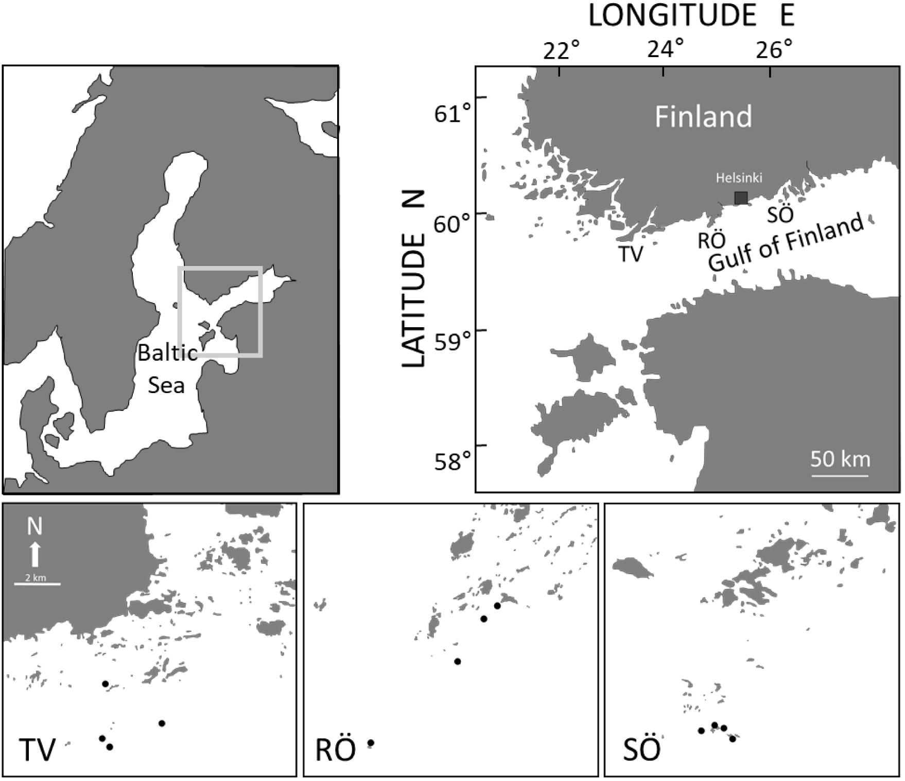
Figure 1. Gulf of Finland and study areas Tvärminne (TV), Rönnskär (RÖ), and Söderskär (SÖ). Distance between areas ca 130 km. Sampling stations are shown in the lower panel. The scale is equal among all figures in the lower panel.
Salinity, Temperature, and Sea Ice Data
Decadal (1970–2017) and frequently sampled environmental data including sea surface salinity and temperature were extracted from two national coastal water monitoring stations (UUS10A and UUS23) at different ends of the study area to provide indications for long-term salinity and temperature evolution. For mussel distribution modeling, we used salinity data sampled in May and temperature data sampled in August (one measurement station–1 year–1) from the closest available national monitoring stations [UUS23 (TV), Stora Mickelskären (RO), and UUS10A (SO)]. The distance from the national water monitoring stations to the three sampling areas varies from ca 3 km at TV to ca 15 km at RO and SO. We used May values for salinity as low salinity conditions were anticipated to affect reproduction success (either directly through larval condition or indirectly through gonad development, gonad condition and reproductive output) and as May coincides with annual salinity low and with the onset of the spawning period (Kautsky, 1982). In the Gulf of Finland, blue mussels show the highest seasonal salinity stress during the late spring period (Leiniö and Lehtonen, 2005). Such increased stress may lead to increased mortality of particularly larvae and juveniles or lead to a lower adult investment in reproduction that would show lagged changes in population metrics. Since only high temperatures were expected to affect populations (Fly and Hilbish, 2013), August measurements were used as they coincide with the annual temperature high. To test the influence of salinity and temperature on recruits and adults at year y, we used y–1 salinity and temperature measurements that showed the strongest response in linear mixed effects models and its backward stepwise model reduction procedure. To estimate the effects of sea ice disturbance, we used the Baltic ice extent data (km2, see, e.g., Omstedt et al., 2014) provided by the Finnish Meteorological Institute as a proxy for winter severity. The Baltic ice extent is strongly related to winter conditions (Omstedt et al., 2014).
Sampling Design
To examine population structure, abundance and biomass of M. trossulus, 48 quadrates, 400 cm–2, were sampled (SCUBA) in late May – late June during the period 1996–2005 from each of the three areas. In 1996, samples were taken from 8 m only and the available data is only used as a descriptive baseline for the study. In 2000, no samples were taken. Using a metal frame with one side ending in a net bag (mesh < 0.1 mm), benthic samples were collected from stations in the outer archipelago area (Figure 1). In each area, four haphazardly selected sampling stations were selected. Depth profiles, wave exposure and substrate quality were used as criteria to standardize stations among areas as best possible. Only stations with rocky slopes were included. Stations were further selected so that the deepest sampling depth was reached within 100 m from the shoreline (safety regulations when diving with only one diver). Using these as selection criteria and avoiding very proximate stations, neighboring stations, within areas, were dispersed by a distance of ca. <1–5 km within areas. At each station, three replicates, dispersed by 10–20 m, were randomly taken from each of four depths: 3, 5, 8, and 12 m. Hence, 48 annual quadrates were obtained for each study area (sample total = 1137 excluding samples from 1996). The sampling areas represent typical hard bottoms of the outer archipelago where the outermost islets and reefs meet the open sea (Figure 1). Within areas, wave exposure is the most significant factor affecting population size (e.g., Westerbom and Jattu, 2006). Therefore, also wave exposure was an important variable to standardize among areas and it was indifferent between areas (Kruskal–Wallis, H = 0.16, df = 2, P = 0.93). The same SCUBA divers (MW and OM) collected samples throughout the study, thus minimizing biases caused by interpersonal differences in sampling.
Sample Processing
In the laboratory, samples were sequentially passed through 9.5, 4, 2, and 1 mm sieves. Upon sieving, mussels were emptied on trays and counted. To obtain an accurate assessment of size distributions and biomass, subsamples from each station and year were randomly selected and measured for length to the nearest 0.1 mm using calipers. This was done as data originating from sieves only roughly grouped mussels into coarse and partly overlapping size classes and as sieving alone doesn’t separate mussels in an equal manner among samples (the effectiveness of sieving depends, e.g., on how much material there is in each sample). Based on the measured mussel size distribution from random subsamples, mussel count data originating from sieves was converted into size distribution data that was rounded to the nearest 1 mm in mussel length. As the discrete count data from the sieves was transformed into 1 mm size classes, and as the transformation to each mm group was done based on the ratio of different mussel lengths from subsamples (not the total), the discrete count data from sieves turned into a continuous variable. When differences in size distribution among samples were large, the procedure was repeated also among depths and samples. Based on these measurements, sample biomasses (flesh DW) were counted (Westerbom et al., 2002) and mussels were categorized into two operational classes – recruits and adults.
Definition of Recruits and Adults
Recruitment is an operational term, rather than a biological event, and the definition varies highly among studies (Booth and Brosnan, 1995). We define recruits as individuals with a length of 2–3.5 mm that mainly correspond to individuals with an age of 1–2 years (Antsulevich et al., 1999; Westerbom et al., 2002) but that have not yet reached adulthood (Kautsky, 1982). Correspondingly, adults are defined as individuals larger than 3.5 mm.
Data Analysis
To test changes or differences in background environmental parameters, parametric tests (ANOVA, t-test and Pearson’s correlation) were conducted. When assumptions of normality, linearity (Pearson’s) and variance homogeneity were not met (even after transformations), non-parametric tests were used (Kruskal–Wallis and Spearman’s rho).
To study the influence of environmental variables on the abundance of both recruits and adult mussels, we constructed two linear mixed effects models (LMM) where the abundance of recruits or adults were explained by area (entered as a factor with the levels TV, RÖ, and SÖ), summer water temperature, salinity, wave exposure, depth, and sea-ice extent. The abundance of adult mussels was added to the model describing the abundance of recruits, since adult mussels serve as a settling structure for recruits. We used station nested within study area as a random effect in the models to account for potential pseudoreplication arising from repeated observations within station and study area. To study differences in responses of recruit or adult abundance to environmental variables among the study areas, two-way interactions between study area and environmental variables were entered in the models. Models were fitted using restricted maximum likelihood. Although representing an abundance of individuals, the response variables in these analyses adhere to a normal distribution and not a Poisson distribution due to the size class assignment procedure during counting of mussel abundance that produces continuous data (see section “Sample Processing”).
For the residuals of both models, and to adhere to the assumption of normality, the abundances of both recruits and adults were square root transformed. Model selection was done by removing all non-significant variables (α = 0.05) using backward stepwise model reduction, where the least significant covariates were removed one at a time until the model contained only significant variables and interactions. Here we used an X2 analysis of deviance with type II sums of squares, which is not sensitive to the order of the covariates in the model (Langsrud, 2003). When significant interactions were detected, the area-specific slopes for each covariate was tested using a covariate-specific t-test. All statistical analyses were performed using the software RStudio 1.0.136 (R Core Team, 2016).
Results
Long-Term Environmental Trends
A significant and highly correlated 40-year trend of declining seawater salinity is shown throughout the study area (Pearson r = 0.84, P < 0.001). This trend corresponds to a westward geographic shift in the average salinity regime of 50–100 km and an average decline of 0.5 g kg–1 along the gradient (Figure 2A). Since the 1970s, seawater temperature has risen by 3–4°C in the study area showing no differences between the two monitoring stations (t-test −0.23, P = 0.82, Figure 2B).
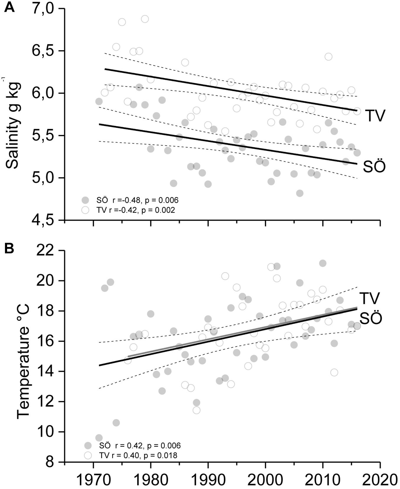
Figure 2. Long-term salinity (A) (annual mean) and temperature (B) (August) trends with 95% confidence intervals at Tvärminne (TV) and Söderskär (SÖ) in the western and central Gulf of Finland.
Mussel Population Trends
A single synchronous and massive recruitment peak was recorded in 1998 that triggered population growth in all areas. The recruitment event was preceded by a marked rise in salinity in 1997 throughout the study area (Figure 3A). The event caused an increase in adult numbers in all areas but the size of population growth was area specific reaching a peak earlier in the peripheral east compared to the west (Figure 3A). The population size showed a fourfold change between low and high years at TV, eightfold at RÖ and 64-fold at SÖ. Recruitment showed moderate synchrony between areas and years (TV-RÖ, Spearman rs = 0.54, TV-SÖ rs = 0.39, RÖ-SÖ rs = 0.49, P < 0.001 in all cases), whereas the temporal relation in adult abundances was lower (TV-RÖ rs = 0.38, P < 0.001, TV-SÖ rs = 0.06, P = 0.23, RÖ-SÖ rs = 0.27, P < 0.001). Populations differed highly in biomass, showing consistently lower biomass from west to east and a threshold of change in biomass between TV and RÖ where biomasses dropped by more than 80% over a salinity change of merely 0.5 g kg–1 (Figure 3B).
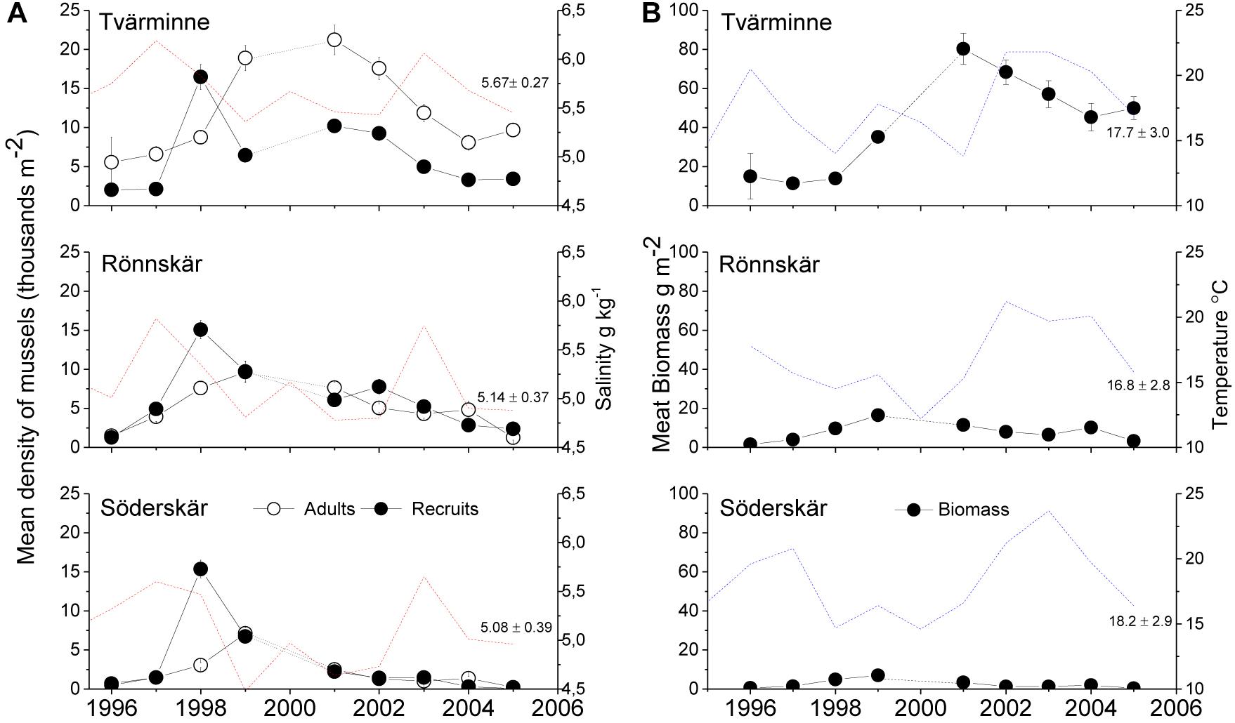
Figure 3. Mean density ( ± SE) of adult mussels and recruits at the three study areas (A) 1996–2005 and concomitant changes in salinity and temperature. Salinity (May) and temperatures changes (August) during the study period are also shown, as well as mean ± SD for the entire period). Mean ( ± SE) biomass at the three study areas is shown in the right panel (B). Between 1995 and 2005 salinity was higher at Tvärminne compared to Rönnskär and Söderskär (ANOVA, F2,27 = 11.1, P < 0.001), whereas temperature (1996–2005, as RO lacked temperature data in 1995) was similar among areas (ANOVA, F2,24 = 0.74, P = 0.5).A clear spatial tipping point is seen between TV and RÖ where long-term salinity declines by ca 0.5 g kg–1, but shows a > 5-fold drop in average biomass.
Recruit Dynamics
The abundance of recruits was significantly related to the covariates summer water temperature and wave exposure and by interactions between area and the covariates: salinity, winter severity, depth, and adult abundance (Supplementary Table S1). The fixed effects in the model explained a high proportion of the variation in the data with a marginal R2 value of 0.45. The negative effect of summer temperature (b = −0.47, 2 = 52.29, df = 1, P < 0.0001) and the lack of an interaction between area and temperature shows that the effect of temperature on recruit abundance had a uniform effect across the area (Figure 4A). Similarly, the effect of wave exposure was uniformly positive (b = 0.30, 2 = 18.16, df = 1, P < 0.0001). Salinity had a positive effect on recruit abundance across the study area, but the strength of the effect differed among areas, as shown by the significant interaction between area and salinity (b = 2.55, 2 = 8.53, df = 1, P = 0.003; Figure 4B). This interaction shows that salinity affects recruitment strongest at SÖ (b = 12.79, t1112 = 12.36, P < 0.0001) and TV (b = 12.33, t1112 = 8.32, P < 0.0001) and weaker at RÖ (b = 3.59, t1112 = 4.07, P < 0.0001). The extent of sea ice affected recruit abundance negatively across the entire study area, but the strength of the effect differed among areas, as shown by the significant interaction between area and the extent of sea ice (b = −0.00001, 2 = 7.22, df = 1, P = 0.007; Figure 4C) with strongest effects at SÖ (b = −0.00006, t1112 = −9.36, P < 0.0001) followed by TV (b = −0.00005, t1112 = −7.36, P < 0.0001) and RÖ (b = −0.00003, t1112 = −4.99, P < 0.0001). The effect sizes of this interaction were modest, indicating an almost uniform effect across the study area. Depth had a disparate effect on recruit abundance at different areas (b = 0.19, 2 = 7.18, df = 1, P = 0.007) as recruits decreased with depth at TV (b = −0.34, t1112 = −3.30, P < 0.0001) but showed no effects at RÖ (b = 0.01, t1112 = 0.12, P = 0.90) or SÖ (b = 0.11, t1112 = 1.16, P = 0.25).
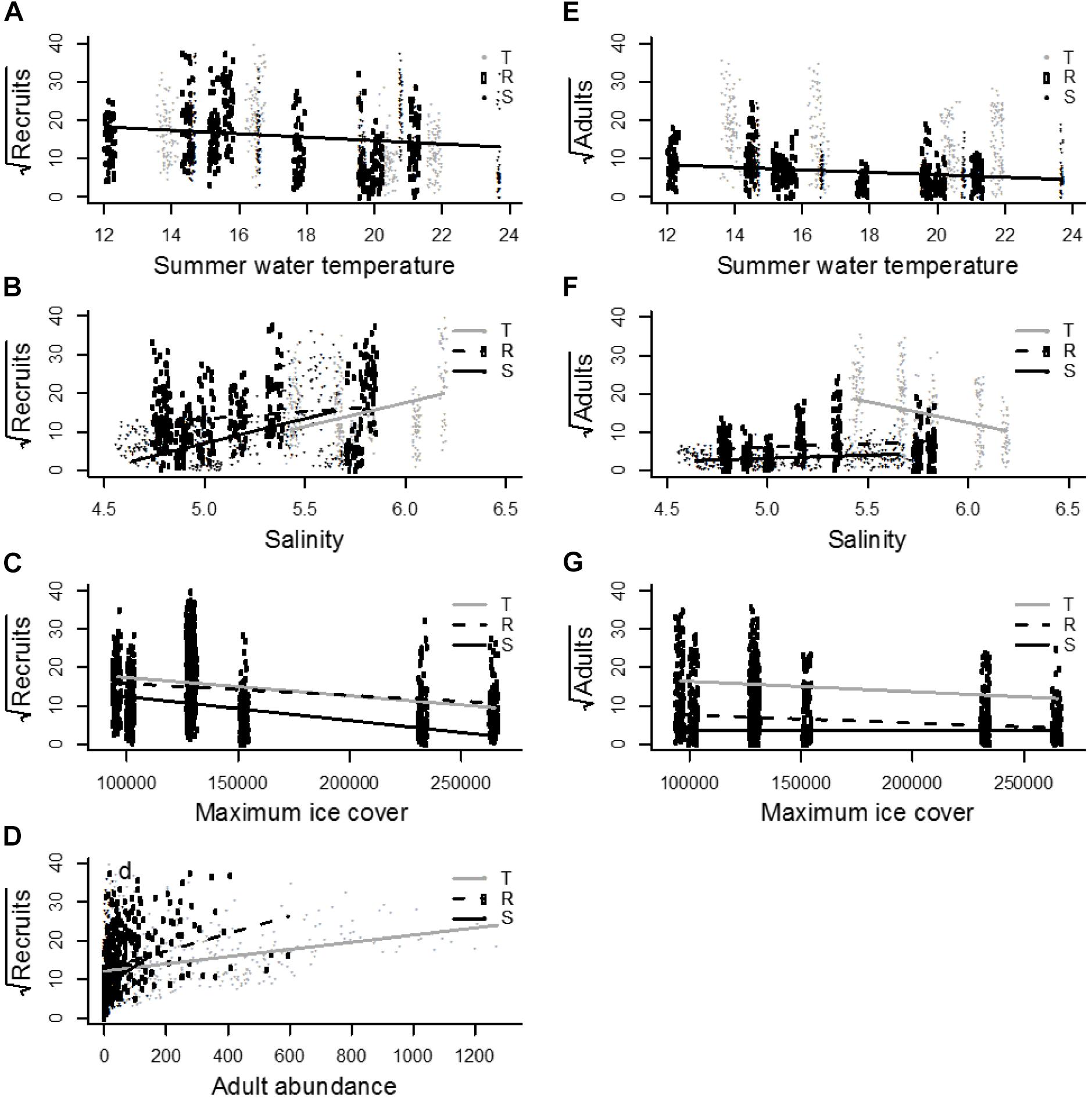
Figure 4. August water temperature had a uniform and negative effect on both recruits (A) and adults (E). (B) Salinity had a positive effect on the number of recruits in all areas. (C) Severe ice winters (unit is km2) decreased the number of recruits with the strongest effect at Söderskär and affected negatively adults at TV and RÖ, but was insignificant at SÖ (G). (D) Adult abundance had a positive effect on the number of recruits at all areas with an increase in the strength of this effect from Tvärminne to Söderskär. (F) Salinity had a positive effect on the number of adult mussels at Söderskär and Rönnskär but not at Tvärminne.
The abundance of adults affected recruit abundance positively throughout the study area. Yet a significant interaction term showed that the strength of the effect differed among areas (b = 0.01, 2 = 12.52, df = 1, P = 0.0004; Figure 4D), with the strongest effect of adult abundance on recruits at SÖ (b = 0.05, t1112 = 2.96, P = 0.003), followed by RÖ (b = 0.02, t1112 = 5.67, P < 0.0001) and TV where the effect was weakest (b = 0.009, t1112 = 5.99, P < 0.0001).
Adult Dynamics
Adult abundance was significantly related to summer water temperature and the interactions between area and the following covariates: salinity, winter severity, wave exposure, and depth (Supplementary Table S1). The fixed effects in the model explained a high proportion of the variation in adult abundance, with a marginal R2 value of 0.65. Summer water temperature had a spatially uniform, significant negative effect on adult abundance across the study area (b = −0.37, 2 = 59.34, df = 1, P < 0.0001; Figure 4E). A significant interaction term between area and salinity showed that salinity effects were area specific (b = 5.30, 2 = 81.97, df = 1, P < 0.0001; Figure 4F). Salinity had a positive effect on adult abundance at SÖ (b = 1.64, t1115 = 2.39, P = 0.02) and RÖ (b = 1.78, t1115 = 3.01, P = 0.003), but a negative effect at TV (b = −10.98, t1115 = −11.65, P < 0.0001). A significant interaction between winter severity and area showed that ice effects differed among areas (b = 0.00001, 2 = 18.23, df = 1, P < 0.0001; Figure 4G) with adult abundances decreasing during harsh winters at TV (b = −0.00003, t1115 = −6.33, P < 0.0001) and RÖ (b = −0.00002, t1115 = −4.97, P < 0.0001), but showing no significant effect at SÖ (b < −0.00001, t1115 = 0.01, P = 0.99). The effect sizes of this interaction were, however, modest, indicating an almost uniform effect over the study area. The effect of wave exposure differed between areas, as indicated by the significant interaction term (b = −0.32, 2 = 11.74, df = 1, P = 0.0006). Adult abundance increased with increasing wave exposure at TV (b = 0.80, t6 = 6.69, P = 0.0005) and RÖ (b = 0.20, t6 = 2.65, P = 0.04), but showed no significant effect at SÖ (b = 0.09, t6 = 0.93, P = 0.39). Finally, the effect of depth on adult abundance differed among areas (b = −0.41, 2 = 75.81, df = 1, P < 0.0001). At TV, increasing depth affected adult abundances negatively (b = 0.73, t1115 = 11.15, P < 0.0001), whereas no significant depth effects were observed at RÖ (b = 0.04, t1115 = 0.63, P = 0.53) or SÖ (b = −0.10, t1115 = −1.51, P = 0.13).
Discussion
Here we significantly extend previous snapshot assessments of spatial distribution patterns of Baltic Sea blue mussels along environmental gradients (e.g., Westerbom et al., 2002; Nyström Sandman et al., 2013; Kotta et al., 2015) by adding time into the spatial analysis. While not sampling the entire range, our areas that were spaced along a salinity gradient, showed responses that fit the central-marginal prediction (e.g., Hengeveld and Haeck, 1982). First, abundances declined toward the range edge at SÖ, paralleling concurrent changes in salinity. According to the central-marginal prediction, environmental gradients cause species to be abundant where species encounter favorable conditions and they decline where conditions become less favorable (Hengeveld and Haeck, 1982; Gaston, 2009). We showed that only subtle changes in salinity caused abrupt declines in abundance, which were manifested in space as well as in time. This suggests that the transition from favorable to unfavorable (or spatially from core to periphery) doesn’t necessarily stem from large environmental changes but arises from small fluctuations around critical thresholds (Welch et al., 1995; Sagarin et al., 2006; Chang et al., 2018). Identifying the location of such tipping points along environmental gradients is critically important as they may unlock the mechanisms for change and provide projections for whole-scale community development in a changing climate (Chang et al., 2018). Second, the survival of recruits was much lower at the range edge, which was also manifested as a constantly low biomass, despite an equally sized recruitment pulse in 1998 throughout the area. Longevity and size of individuals should decrease toward the margin, because here resources are increasingly allocated to homeostasis instead of allocated to somatic growth (Samis and Eckert, 2007, see however Tam and Scrosati, 2011). Even if the abundant center model cannot be tested on this data because of the limited geographical coverage, we show that the model and its fundamental assumptions can (1) provide insights into understanding the mechanisms affecting distribution patterns of mussels in this marginal area and (2) provide predictions for population specific responses. We also show that abundances are high throughout the range in some years, showing a distribution pattern that contrasts the prediction. This strengthens the notion that investigating distribution patterns in the margin asks for the inclusion of time, as single observations may deviate highly from the average pattern (e.g., Sexton et al., 2009). In addition, we show that critical tipping points may remain undetected in one-off spatial surveys as the location of such tipping points may be revealed only over time.
At the edge therefore, recruitment may be highly variable and recruit mortality high, preventing new recruits from entering the adult population in most years (Zacherl et al., 2003; Sorte et al., 2017). Occasionally however, this general pattern may break down by sporadic recruitment causing a narrowing of the traditional bell-shaped center-periphery pattern. Such synchronous recruitment over distant populations may be caused either by larval supply or by environmental drivers that are spatially synchronized (Liebhold et al., 2004). Synchronic recruitment patterns have been demonstrated in terrestrial and marine systems, spanning, e.g., valley oaks (Koenig et al., 2017), caribou and musk oxen (Post and Forchhammer, 2002), kelps (Cavanaugh et al., 2013), fish (Kelly et al., 2009; Weber et al., 2017), oysters (Wasson et al., 2016), clams (Beukema et al., 2010, 2017), and barnacles (Burrows et al., 2002; Lagos et al., 2007). Understanding the mechanism causing synchronic recruitment at range edges is important as it may explain the setting of the range boundary (Gaston, 2009). Here we showed that recruitment pulses caused sporadic but ephemeral replenishment of populations, particularly at the very range edge (see also Zacherl et al., 2003). We identified a single peak in recruitment that was uniform in strength over the entire gradient, indicating a large-scale process that triggered an identical response in the three disparate populations. This synchronous and equally sized recruitment event across the area, suggests that propagule delivery processes are important for structuring and maintaining the studied populations, especially at the very range edge. Delivery dynamics may also explain the lack of recruitment response in 2004, when sea salinity was exceptionally high in the entire Gulf of Finland in 2003. In addition to very warm waters in July and August that may have had a negative effect, exceptionally strong and consistent eastward winds prevailed the summer months of 2003 (Jouni Lehtoranta, personal communication) that possibly prevented recruit arrival, especially in the eastern areas. Our results also indicate that population longevity is driven by the local climate as recruits were increasingly short-lived toward the edge causing only a short temporal increase in the adult population size (Figure 3). These findings reinforce earlier comparisons showing that source populations can maintain marginal sink populations that collapse without immigration (Pulliam, 1988; Wilson et al., 2002). In dispersal mediated range edges, average individuals are often smaller at the range edge as recruits dominate the populations. At SÖ, we saw highly variable recruitment over time, a high share of recruits in all years and a very low storage potential over the years. These combined results suggest that the edge in this marginal area (SÖ) is populated because of sporadic immigration events from more central areas (Figure 3) whereas a more even recruitment over time away from the edge suggest either local net production, higher survival of recruits or a shorter distance to the possible source. Variation in individual growth rate among the studied areas is not a factor that explains differences in population growth rate (Westerbom et al., 2002).
Blue mussels are euryhaline osmoconformers (Tedengren and Kautsky, 1986) with minimum salinity requirements around 5 g kg–1 (e.g., Vuorinen et al., 2015). Here we showed that recruitment was positively affected by salinity in all areas. Salinity also explained adult numbers at SÖ and RÖ, but surprisingly showed a negative effect at TV. This negative effect is likely an artifact of few adults in the beginning of the study when salinity was high and high number of adults at the later stages of the study when salinity was lower, reflecting different storage potential (history) between areas rather than effects of salinity on adult survival at TV.
The effects of temperature alone on mussel condition and populations is well-documented and thermal stress is considered one of the strongest mechanisms setting species range limits (Jones et al., 2010; Sorte et al., 2017). Environmental stress caused by temperature or salinity can strongly affect the energy balance of an organism due to the additional energy needed to maintain homeostasis with most distinct effects in low food regimes (Schneider et al., 2010). Fly and Hilbish (2013) showed that the energetic balance of M. trossulus turns unfavorable above 17°C and that the geographic range of the species largely follows areas with maximum annual temperatures ranging between 15 and 20°C. Such temperatures are common during the late summer peak in the Baltic Sea (Figure 3B), likely causing temperature stress during warm summers that on top of continuous salinity stress may cause increased mortality during heat periods. Here, adult and recruit abundance were negatively affected by high temperatures indicating a uniform population level and life history effect of high water temperatures throughout the range.
Adult conspecifics had a positive effect on recruit abundance throughout the range and the effect size increased toward the range margin where adults were few. As adults form the habitat for early recruits (e.g., McGrath et al., 1988), a shortage of adults may affect future population size. Therefore, toward the eastern margin, declines in adult coverage can have negative effects on mussel replenishment suggesting that declines or extirpations are not readily reversible. Hence, degradation of adult populations may jeopardize recovery processes and lead to permanently low recruitment and a treadmill-process of periods of weak and ephemeral recovery followed by periods of severe declines. It is also possible that the decreasing facilitation effect toward the west is a result of a balancing process between positive and negative density-dependency where positive effects of environment quality are counteracted by negative adult competition effects. The stronger positive effect of adults on recruit survival toward the margin may therefore be a consequence of lower resource competition, which may mask other density-dependent mechanisms that become more important toward the west where adult abundances are high.
We have shown the effects of high temperatures and low salinity on mussel dynamics, but environmental changes are only on their rise; reduced salinity and increases in temperature have already been observed (Figure 2), with clear repercussions for mussels as shown in this study. A warmer climate may reduce winter severity through reduced ice scouring effects (Figure 4), but warmer winters may also come with many other effects, including increased metabolic demand (e.g., Beukema et al., 2017). Climate change forecasts predict a continued and escalating warming of the Baltic Sea. Summer surface water temperature increases by 4°C by the end of this century have been anticipated (Meier, 2006; BACC II Author Team, 2015). Such changes would alone cause prolonged periods of energetically stressful temperatures (Fly and Hilbish, 2013), that likely would be intensified along with other changes in the sea. Predictions for future salinities are uncertain, but suggest a continued freshening of the sea (Meier et al., 2012; BACC II Author Team, 2015). Meier (2006) predicted a decline in salinity in the range 8–50% within the next century. Changes at the lower end of the scenarios would push the range limit westward and future structure at TV would be somewhat comparable with those at current SÖ. Predictions at the upper end would likely push mussels out from the entire northern Baltic Sea. Population density and structure changes would also be caused by alternate drivers that are linked to altered salinity or temperature levels such as changes in food composition or food-quality and alterations in predator pressure (Westerbom et al., 2018). This raises the question of how populations and their distribution will continue to change and the ecological consequences of shifting abundances. Given the decisive role Baltic blue mussels have for ecosystem health and ecosystem resilience; any shift in abundance and distribution will cascade through the ecosystem causing radical alterations in entire communities including several Baltic Sea flag ship species.
Data Availability
The datasets generated for this study are available on request to the corresponding author.
Ethics Statement
This study was carried out in accordance with the current laws in Finland. There are no legal or ethical restrictions involving benthic invertebrates.
Author Contributions
MW, OM, and MK designed the study. MW and OM collected data. KJ and MW analyzed data. MW and KJ wrote a draft of the manuscript. All authors contributed to the revision of the work.
Funding
The dataset was a result of a private activity and endeavor including > 2500 person-hours for which funding was partially covered by Walter and Andrée de Nottbecks Foundation (MW and OM), Svenska Kulturfonden (AN, KJ, and MW) and Academy of Finland (MW) (Project No. 126831).
Conflict of Interest Statement
The authors declare that the research was conducted in the absence of any commercial or financial relationships that could be construed as a potential conflict of interest.
Acknowledgments
We thank Martti Hario for all help at Söderskär. We are grateful to Nils Kautsky for comments on an earlier version of this manuscript. Jukka Lehtonen, Avi Rahman, Eva Sjöblom, and Malin Sandberg assisted in field and laboratory. Valuable comments by the two reviewers helped us much to clarify the manuscript.
Supplementary Material
The Supplementary Material for this article can be found online at: https://www.frontiersin.org/articles/10.3389/fmars.2019.00292/full#supplementary-material
TABLE S1 | Results of the linear mixed-effects models (LMMs) testing the influence of environmental variables on the abundance of recruits and adults.
References
Antsulevich, A., Maximovich, N., and Vuorinen, I. (1999). Population structure growth and reproduction of the common mussel (Mytilus edulis L.) off the Island of Seili (SW Finland). Bor. Environ. Res. 4, 367–375.
BACC II Author Team (2015). Second Assessment of Climate Change for the Baltic Sea Basin. New York, NY: Springer International Publishing.
Bates, A. E., Pecl, G. T., Frusher, S., Hobday, A. J., Wernberg, T., Smale, D. A., et al. (2014). Defining and observing stages of climate-mediated range shifts in marine systems. Glob. Environ. Chang. 26, 27–38. doi: 10.1016/j.gloenvcha.2014.03.009
Belkin, I. M. (2009). Rapid warming of large marine ecosystems. Progr. Oceanogr. 81, 207–213. doi: 10.1016/j.pocean.2009.04.011
Beukema, J. J., Dekker, R., and Drent, J. (2017). Parallel changes of Limecola (Macoma) balthica populations in the Dutch Wadden Sea. Mar. Ecol. Progr. Ser. 585, 71–79. doi: 10.3354/meps12360
Beukema, J. J., Dekker, R., and Philippart, C. J. M. (2010). Long-term variability in bivalve recruitment, mortality, and growth and their contribution to fluctuations in food stocks of shellfish-eating birds. Mar. Ecol. Progr. Ser. 414, 117–130. doi: 10.3354/meps08706
Booth, D. J., and Brosnan, D. M. (1995). The role of recruitment dynamics in rocky shore and coral reef fish communities. Adv. Ecol. Res. 26, 309–385. doi: 10.1016/S0065-2504(08)60068-9
Brown, C. J., Schoeman, D. S., Sydeman, W. J., Brander, K., Buckley, L. B., Burrows, M., et al. (2011). Quantitative approaches in climate change ecology. Glob. Change Biol. 17, 3697–3713. doi: 10.1111/j.1365-2486.2011.02531.x
Burrows, M. T., Moore, J. J., and James, B. (2002). Spatial synchrony of population changes in rocky shore communities in Shetland. Mar. Ecol. Progr. Ser. 240, 39–48. doi: 10.3354/meps240039
Caughley, G., Grice, D., Braker, R., and Brown, B. (1988). The edge of the range. J. Anim. Ecol. 57, 771–785. doi: 10.2307/5092
Cavanaugh, K. C., Kendall, B. E., Siegel, D. A., Reed, D. C., Alberto, F., and Assis, J. (2013). Synchrony in dynamics of giant kelp forests is driven by both local recruitment and regional environmental controls. Ecology 94, 499–509. doi: 10.1890/12-0268.1
Chang, A. L., Brown, C. W., Crooks, J. A., and Ruiz, G. M. (2018). Dry and wet periods drive rapid shifts in community assembly in an estuarine ecosystem. Glob. Change Biol. 24, e627–e642. doi: 10.1111/gcb.13972
Channell, R., and Lomolino, M. V. (2000). Trajectories to extinction, spatial dynamics of the contraction of geographical ranges. J. Biogeogr. 27, 169–179. doi: 10.1046/j.1365-2699.2000.00382.x
Fly, E. K., and Hilbish, T. J. (2013). Physiological energetics and biogeographic range limits of three congeneric mussel species. Oecologia 172, 35–46. doi: 10.1007/s00442-012-2486-6
Fogarty, H. E., Burrows, M. T., Pecl, G. T., Robinson, L. M., and Poloczanska, E. S. (2017). Are fish outside their usual ranges early indicators of climate-driven range shifts? Glob. Change Biol. 23, 2047–2057. doi: 10.1111/gcb.13635
Gaston, K. J. (2009). Geographic range limits: achieving synthesis. Proc. R. Soc. Lond. Ser. B Biol. Sci. 276, 1395–1406. doi: 10.1098/rspb.2008.1480
Goldstein, E., Merrick, M. J., and Koprowski, J. L. (2017). Functional semelparity drives population dynamics and endangers a peripheral population. Biol. Conserv. 205, 52–59. doi: 10.1016/j.biocon.2016.11.017
Grayson, K. L., and Johnson, D. M. (2018). Novel insights on population and range edge dynamics using an unparalleled spatiotemporal record of species invasion. J. Anim. Ecol. 87, 581–593. doi: 10.1111/1365-2656.12755
Halpern, B. S., Gaines, S. D., and Warner, R. R. (2005). Habitat size, recruitment, and longevity as factors limiting population size in stage-structured species. Am. Natural. 165, 82–94. doi: 10.1086/426672
Harley, C. D. G., Hughes, A. R., Hultgren, K. M., Miner, B. G., Sorte, C. J. B., Thornber, C. S., et al. (2006). The impacts of climate change in coastal marine systems. Ecol. Lett. 9, 228–241. doi: 10.1111/j.1461-0248.2005.00871.x
Hengeveld, R., and Haeck, J. (1982). The distribution of abundance. I. measurements. J. Biogeogr. 9, 303–316. doi: 10.2307/2844717
Hewitt, J. E., Ellis, J. I., and Thrush, S. F. (2016). Multiple stressors, nonlinear effects and the implications of climate change impacts on marine coastal ecosystems. Glob. Change Biol. 22, 2665–2675. doi: 10.1111/gcb.13176
Holt, R. D., and Barfield, M. (2003). Impacts of temporal variation on apparent competition and coexistence in open ecosystems. Oikos 101, 49–58. doi: 10.1034/j.1600-0706.2003.12570.x
Huang, Q., Sauer, J. R., and Dubayah, R. O. (2017). Multidirectional abundance shifts among North American birds and the relative influence of multifaceted climate factors. Glob. Change Biol. 23, 3610–3622. doi: 10.1111/gcb.13683
Jones, S. J., Lima, F. P., and Wethey, D. S. (2010). Rising environmental temperatures and biogeography: poleward range contraction of the blue mussel, Mytilus edulis L., in the western Atlantic. J. Biogeogr. 37, 2243–2259. doi: 10.1111/j.1365-2699.2010.02386.x
Kautsky, N. (1982). Quantitative studies on the gonad cycle, fecundity, reproductive output and recruitment in a Baltic Mytilus edulis L. population. Mar. Biol. 68, 143–168. doi: 10.1007/BF00397601
Kelly, J. E., Frank, K. T., and Leggett, W. C. (2009). Degraded recruitment synchrony in Northwest Atlantic cod stocks. Mar. Ecol. Progr. Ser. 393, 131–146. doi: 10.3354/meps08241
Koenig, W. D., Knops, J. M. H., Pesendorfer, M. B., Zaya, D. N., and Ashley, M. V. (2017). Drivers of synchrony of acorn production in the valley oak (Quercus lobata) at two spatial scales. Ecology 98, 3056–3062. doi: 10.1002/ecy.2010
Koivisto, M., and Westerbom, M. (2012). Invertebrate communities associated with blue mussel beds in a patchy environment: a landscape ecology approach. Mar. Ecol. Progr. Ser. 471, 101–110. doi: 10.3354/meps10010
Kotta, J., Oganjan, K., Lauringson, V., Pärnoja, M., Kaasik, A., Rohtla, L. I., et al. (2015). Establishing functional relationships between abiotic environment, macrophyte coverage, resource gradients and the distribution of Mytilus trossulus in a brackish non-tidal environment. PLoS One 10:e0136949. doi: 10.1371/journal.pone.0136949
Lagos, N. A., Tapia, F. J., Navarrete, S. A., and Castilla, J. C. (2007). Spatial synchrony in recruitment of intertidal invertebrates along central Chile. Mar. Ecol. Progr. Ser. 350, 29–39. doi: 10.3354/meps07105
Langsrud, Ø. (2003). ANOVA for unbalanced data: use type II instead of type III sums of squares. Stat. Comp. 13, 163–167. doi: 10.1023/A:1023260610025
Lehikoinen, P., Santangeli, A., Jaatinen, K., Rajasärkkä, A., and Lehikoinen, A. (2019). Protected areas act as a buffer against detrimental effects of climate change — evidence from large-scale, long-term abundance data. Glob. Change Biol. 25, 304–313. doi: 10.1111/gcb.14461
Leiniö, S., and Lehtonen, K. (2005). Seasonal variability in biomarkers in the bivalves Mytilus edulis and Macoma balthica from the northern Baltic Sea. Comp. Biochem. Physiol. 140, 408–421. doi: 10.1016/j.cca.2005.04.005
Lenoir, J., and Svenning, J. C. (2015). Climate-related range shifts — a global multidimensional synthesis and new research directions. Ecography 38, 15–28. doi: 10.1111/ecog.00967
Lewis, J. R., Bowman, R. S., and Williamson, P. (1982). Some geographic components in population dynamics: possibilities and realities in some littoral species. Netherlands J. Sea Res. 16, 18–28. doi: 10.1016/0077-7579(82)90013-8
Liebhold, A., Koenig, W. D., and Bjørnstad, O. N. (2004). Spatial synchrony in population dynamics. Ann. Rev. Ecol. Evolu. Syst. 35, 467–490. doi: 10.1146/annurev.ecolsys.34.011802.132516
McGrath, D., King, P. A., and Gosling, E. M. (1988). Evidence for the direct settlement of Mytilus edulis larvae on adult mussel beds. Mar. Ecol. Progr. Ser. 47, 103–106. doi: 10.3354/meps047103
Meier, H. E. M. (2006). Baltic Sea climate in the late 21st century: a dynamical downscaling approach using two global models and two emission scenarios. Clim. Dyn. 27, 39–68. doi: 10.1007/s00382-006-0124-x
Meier, H. E. M., Hordoir, R., Andersson, H. C., Dieterich, C., Eilola, K., Gustafsson, B. G., et al. (2012). Modeling the combined impact of changing climate and changing nutrient loads on the Baltic Sea environment in an ensemble of transient simulations for 1961–2099. Clim. Dyn. 39, 2421–2441. doi: 10.1007/s00382-012-1339-7
Nyström Sandman, A. N., Wikström, S. A., Blomqvist, M., Kautsky, H., and Isaeus, M. (2013). Scale-dependent influence of environmental variables on species distribution: a case study on five coastal benthic species in the Baltic Sea. Ecography 36, 354–363. doi: 10.1111/j.1600-0587.2012.07053.x
Omstedt, A., Elken, J., Lehmann, A., Leppäranta, M., Meier, H. E. M., Myrberg, K., et al. (2014). Progress in physical oceanography of the Baltic Sea during the 2003–2014 period. Progr. Oceanogr. 128, 139–171. doi: 10.1016/j.pocean.2014.08.010
Pecl, G. T., Araújo, M. B., Bell, J. D., Blanchard, J., Bonebrake, T. C., Chen, I.-C., et al. (2017). Biodiversity redistribution under climate change: Impacts on ecosystems and human well-being. Science 355:eaai9214. doi: 10.1126/science.aai9214
Poloczanska, E. S., Brown, C. J., Sydeman, W. J., Kiessling, W., Schoeman, D. S., Moore, P. J., et al. (2013). Global imprint of climate change on marine life. Nat. Clim. Chang. 2, 919–925. doi: 10.1038/nclimate1958
Post, E., and Forchhammer, M. C. (2002). Synchronization of animal population dynamics by largescale climate. Nature 420, 168–171. doi: 10.1038/nature01064
Pulliam, H. R. (1988). Sources, sinks and population regulation. Am. Natural. 132, 652–661. doi: 10.1086/284880
R Core Team (2016). R: A Language and Environment for Statistical Computing. Vienna: R Foundation for Statistical Computing.
Sagarin, R. D., Gaines, S. D., and Gaylord, B. (2006). Moving beyond assumptions to understand abundance distributions across the ranges of species. Trends Ecol. Evol. 21, 524–530. doi: 10.1016/j.tree.2006.06.008
Samis, K. E., and Eckert, C. G. (2007). Testing the abundant centre model using range-wide demographic surveys of two coastal dune plants. Ecology 88, 1747–1758. doi: 10.1890/06-1153.1
Schneider, K. R., Van Thiel, L. E., and Helmuth, B. (2010). Interactive effects of food availability and aerial body temperature on the survival of two intertidal Mytilus species. J. Ther. Biol. 35, 161–166. doi: 10.1016/j.jtherbio.2010.02.003
Sexton, J. P., McIntyre, P. J. A., Angert, L., and Rice, K. J. (2009). Evolution and ecology of species range limits. Ann. Rev. Ecol. Evol. Syst. 40, 415–436. doi: 10.1146/annurev.ecolsys.110308.120317
Sorte, C. J. B., Davidson, V. E., Franklin, M. C., Benes, K. M., Doellman, M. M., Etter, R. J., et al. (2017). Long-term declines in an intertidal foundation species parallel shifts in community composition. Glob. Change Biol. 23, 341–352. doi: 10.1111/gcb.13425
Sunday, J. M., Bates, A. E., and Dulvy, N. K. (2012). Thermal tolerance and the global redistribution of animals. Nat. Clim. Chang. 2, 686–690. doi: 10.1038/NCLIMATE1539
Tam, J. C., and Scrosati, R. A. (2011). Mussel and dogwhelk distribution along the northwest Atlantic coast: testing predictions derived from the abundant-centre model. J. Biogeogr. 38, 1536–1545. doi: 10.1111/j.1365-2699.2011.02498.x
Tedengren, M., and Kautsky, N. (1986). Comparative study of the physiology and its probable effect on size in blue mussels (Mytilus edulis L.) from the North Sea and the Northern Baltic Proper. Ophelia 25, 147–155. doi: 10.1080/00785326.1986.10429746
Vuorinen, I., Hänninen, J., Rajasilta, M., Laine, P., Eklund, J., Montesino-Pouzols, F., et al. (2015). Scenario simulations of future salinity and ecological consequences in the Baltic Sea and adjacent North Sea areas–implications for environmental monitoring. Ecol. Indic. 50, 169–205. doi: 10.1016/j.ecolind.2014.10.019
Walther, G. R., Post, E., Convey, P., Menzel, A., Parmesan, C., Beebee, T. J., et al. (2002). Ecological responses to recent climate change. Nature 416, 389–395. doi: 10.1038/416389a
Wasson, K., Hughes, B. B., Berriman, J. S., Chang, A. L., Deck, A. K., Dinnel, P. A., et al. (2016). Coast-wide recruitment dynamics of Olympia oysters reveal limited synchrony and multiple predictors of failure. Ecology 97, 3503–3516. doi: 10.1002/ecy.1602
Weber, M. J., Brown, M. L., Wahl, D. H., and Shoupc, D. E. (2017). Quantifying the spatial scale of common carp (Cyprinus carpio) recruitment synchrony. Can. J. Fish. Aqu. Sci. 74, 1682–1691. doi: 10.1139/cjfas-2016-0254
Welch, D. W., Chigirinsky, A. I., and Ishida, Y. (1995). Upper thermal limits on the oceanic distribution of Pacific salmon (Oncorhynchus spp.) in the spring. Can. J. Fish. Aqu. Sci. 52, 489–503. doi: 10.1139/f95-050
Wernberg, T., Bennett, S., Babcock, R. C., de Bettignies, T., Cure, K., Depczynski, M., et al. (2016). Climate- driven regime shift of a temperate marine ecosystem. Science 53, 169–172. doi: 10.1126/science.aad8745
Westerbom, M., and Jattu, S. (2006). Effects of wave exposure on the sublittoral distribution of blue mussels (Mytilus edulis) in a heterogeneous archipelago. Mar. Ecol. Prog. Ser. 306, 191–200. doi: 10.3354/meps306191
Westerbom, M., Kilpi, M., and Mustonen, O. (2002). Blue mussels, Mytilus edulis, at the edge of the range: population structure, growth and biomass along a salinity gradient in the north-eastern Baltic Sea. Mar. Biol. 140, 991–999. doi: 10.1007/s00227-001-0765-6
Westerbom, M., Lappalainen, A., Mustonen, O., and Norkko, A. (2018). Trophic overlap between expanding and contracting fish predators in a range margin undergoing change. Sci. Rep. 8:7895. doi: 10.1038/s41598-018-25745-6
Wilson, R. J., Ellis, S., Baker, J. S., Lineham, M. E., Whitehead, R. W., and Thomas, C. D. (2002). Large-scale patterns of distribution and persistence at the range margins of a butterfly. Ecology 83, 3357–3368. doi: 10.2307/3072085
Keywords: climate variability, environmental gradient, edge of the range, estuarine, rocky shore, synchronized recruitment, monitoring, central-marginal hypothesis
Citation: Westerbom M, Mustonen O, Jaatinen K, Kilpi M and Norkko A (2019) Population Dynamics at the Range Margin: Implications of Climate Change on Sublittoral Blue Mussels (Mytilus trossulus). Front. Mar. Sci. 6:292. doi: 10.3389/fmars.2019.00292
Received: 06 March 2019; Accepted: 20 May 2019;
Published: 07 June 2019.
Edited by:
Paul E. Renaud, Akvaplan-niva, NorwayReviewed by:
Alexey Sukhotin, Zoological Institute (RAS), RussiaJakob Thyrring, British Antarctic Survey (BAS), United Kingdom
Copyright © 2019 Westerbom, Mustonen, Jaatinen, Kilpi and Norkko. This is an open-access article distributed under the terms of the Creative Commons Attribution License (CC BY). The use, distribution or reproduction in other forums is permitted, provided the original author(s) and the copyright owner(s) are credited and that the original publication in this journal is cited, in accordance with accepted academic practice. No use, distribution or reproduction is permitted which does not comply with these terms.
*Correspondence: Mats Westerbom, bWF0cy53ZXN0ZXJib21AaGVsc2lua2kuZmk=; bXdlc3RlcmJvbUBnbWFpbC5jb20=