 Thomas J. Ryan-Keogh
 Sandy J. Thomalla
- 1Southern Ocean Carbon and Climate Observatory, Smart Places, Council of Scientific and Industrial Research, Cape Town, South Africa
- 2Marine Research Institute, Department of Oceanography, University of Cape Town, Cape Town, South Africa
Chlorophyll fluorescence, primarily used to derive phytoplankton biomass, has long been an underutilized source of information on phytoplankton physiology. Diel fluctuations in chlorophyll fluorescence are affected by both photosynthetic efficiency and non-photochemical quenching (NPQ), where NPQ is a decrease in fluorescence through the dissipation of excess energy as heat. NPQ variability is linked to iron and light availability, and has the potential to provide important diagnostic information on phytoplankton physiology. Here we establish a relationship between NPQsv (Stern-Volmer NPQ) and indices of iron limitation from nutrient addition experiments in the sub-Antarctic zone (SAZ) of the Atlantic Southern Ocean, through the derivation of NPQmax (the maximum NPQsv value) and αNPQ (the light limited slope of NPQsv). Significant differences were found for both Fv/Fm and αNPQ for iron versus control treatments, with no significant differences for NPQmax. Similar results from CTDs indicated that changes in NPQ were driven by increasing light availability from late July to December, but by both iron and light from January to February. We propose here that variability in αNPQ, which has removed the effect of light availability, can potentially be used as a proxy for iron limitation (as shown here for the Atlantic SAZ), with higher values being associated with greater iron stress. This approach was transferred to data from a buoyancy glider deployment at the same location by utilizing the degree of fluorescence quenching as a proxy for NPQGlider, which was plotted against in situ light to determine αNPQ. Seasonal increases in αNPQ are consistent with increased light availability, shoaling of the mixed layer depth (MLD) and anticipated seasonal iron limitation. The transition from winter to summer, when positive net heat flux dominates stratification, was coincident with a 24% increase in αNPQ variability and a switch in the dominant driver from incident PAR to MLD. The dominant scales of αNPQ variability are consistent with fine scale variability in MLD and a significant positive relationship was observed between these two at a ∼10 day window. The results emphasize the important role of fine scale dynamics in driving iron supply, particularly in summer when this micronutrient is limiting.
Introduction
Chlorophyll fluorescence has previously been adopted as a proxy for chlorophyll concentration (Lorenzen, 1966), however accurately measuring and interpreting these data is not trivial, in particular during daytime periods of high irradiance when fluorescence is depressed and no longer correlated with chlorophyll (Yentsch and Ryther, 1957; Slovacek and Hannan, 1977; Owens et al., 1980; Abbott et al., 1982; Falkowski and Kolber, 1995). These diel fluctuations in chlorophyll fluorescence are caused by a decrease in the fluorescence quantum yield when light energy absorption exceeds the photosynthetic capacity for light utilization (Müller et al., 2001; Behrenfeld et al., 2009). The resultant decrease in the ratio of photons emitted as fluorescence to those absorbed by photosynthetic pigments is a process termed non-photochemical quenching (NPQ) (Kiefer, 1973; Cullen, 1982; Falkowski and Kolber, 1995; Sackmann et al., 2008), whereby excess energy is dissipated as heat at the cost of fluorescence (Milligan et al., 2012) as a mechanism to protect the photosynthetic apparatus (Demmig-Adams and Adams, 1996). If fluorescence quenching is not corrected, daytime fluorescence will generate under-representative approximations of chlorophyll concentrations (Biermann et al., 2015), which is a major concern for generating long-term, high quality datasets from which trends of climatic relevance can be ascertained (Xing et al., 2012). Despite the hindrance to accurate chlorophyll estimates, this physiological variability within NPQ has the potential to provide important information on phytoplankton photosynthetic efficiency.
Non-photochemical quenching, which can originate in either the light-harvesting antenna or the photosynthetic reaction center (Falkowski and Raven, 2007), is known to vary in response to light under saturating conditions (Milligan et al., 2012; O’Malley et al., 2014; Schuback et al., 2016), to changes in community structure (Kropuenske et al., 2009), and to iron limiting conditions (Schallenberg et al., 2008, 2020; Alderkamp et al., 2012; Schuback et al., 2015). An empirical relationship with SST has also been described (Browning et al., 2014), however the underlying controls of this relationship are still not entirely understood. Derivation of NPQ in situ has typically consisted of measurements of active chlorophyll fluorescence alongside the derivation of the maximum quantum yield of photosystem II, Fv/Fm, which has long been established as a key physiological indicator of phytoplankton, and in particular the significant decreases that occur under conditions of iron limitation (Geider, 1993; Moore et al., 2007). Measurements of both NPQ and Fv/Fm are routinely performed using active fluorometers, however these are currently not readily available to be deployed on autonomous platforms. Instead, autonomous platforms, ships’ underway systems, and CTD rosette systems typically employ standard fluorometers in a capacity to estimate phytoplankton biomass and distribution. This fluorescence is then corrected for quenching to derive chlorophyll, a key ecosystem Essential Ocean Variable (Constable et al., 2016). Whilst Fv/Fm cannot yet be routinely measured on autonomous platforms, if quenching is corrected then the degree of quenching can provide useful information on NPQ.
There are various quenching correction methods that exist in the literature (Sackmann et al., 2008; Xing et al., 2012; Biermann et al., 2015; Hemsley et al., 2015; Swart et al., 2015), however, the optimized method proposed by Thomalla et al. (2018) reduces the reliance on various assumptions and was shown to perform best across multiple oceanic scenarios in the Southern Ocean, including regions dominated by a deep chlorophyll maxima.
Utilization of data from autonomous platforms is at the forefront of oceanographic exploration as these platforms are able to address the space-time gaps of a hitherto radically undersampled ocean. Such measurements are required to improve estimates of phytoplankton biomass and distribution, however an assessment of photosynthetic efficiency on similar scales is also necessary for improved validation of biogeochemical models of oceanic productivity. This is of particular importance in the Southern Ocean where iron limitation is prevalent (Boyd et al., 2007; Moore et al., 2013; Ryan-Keogh et al., 2018b), and the effects of iron limitation on primary production models is poorly constrained (Hiscock et al., 2008; Ryan-Keogh et al., 2017). Here, we utilize iron addition incubation experiments to estimate the effect of iron limitation upon NPQ capacity, along with in situ measurements at a single location in the sub-Antarctic Zone (SAZ). We then use the degree of quenching as a proxy for realized in situ NPQ from standard fluorometers on autonomous platforms to infer iron limitation in the Southern Ocean.
Materials and Methods
Experimental data were obtained as part of the third Southern Ocean Seasonal Cycle Experiment (SOSCEx III) (Swart et al., 2012) on two cruises to the Atlantic sector of the Southern Ocean during winter (July 2015) and summer (December 2015–February 2016). The cruises were onboard the SA Agulhas II, and were spanned by continuous high resolution robotics-based observations in the SAZ. Iron addition incubation experiments were performed as described in Ryan-Keogh et al. (2018a). Briefly, water for incubation experiments was collected from the mixed layer using a trace metal clean CTD rosette system with GoFlo bottles, whereas water for CTD profiles was collected from a CTD rosette system with Niskin bottles at the same location. Experiments were run for 144–168 h in light and temperature-controlled fridge incubators, with two treatments per experiment, an iron addition (+2.0 nM Fe) and a control. Results from experiment 1 from Ryan-Keogh et al. (2018b) where there was no evidence of iron limitation, were excluded from further analysis, as were measurements beyond 120 h from experiments 2 and 3 (where bottle effects and community structure changes were prominent). Samples for active chlorophyll fluorescence light curves (FLCs) were collected at various time points of the experiments from 1 bottle per treatment. Profiles of dissolved iron (DFe) concentrations were collected at the same locations as the incubation experiments. For the detailed methodology of collection and analysis see Mtshali et al. (2019).
Fluorescence light curves were performed using a Chelsea Scientific Instruments FastOceanTM fast repetition rate fluorometer (FRRf) integrated with a FastActTM laboratory system. Samples were dark acclimated for 30 min at incubation temperatures, and measurements were blank corrected using carefully prepared 0.2 μm filtrates (Cullen and Davis, 2003). Active chlorophyll fluorescence measurements consisted of a single turnover protocol with a saturation sequence (100 × 1 μs flashlets with a 2 μs interval) and a relaxation sequence (25 × 1 μs flashlets with an interval of 84 μs), with a sequence interval of 100 ms which was repeated 32 times resulting in a total acquisition time of 3.2 s. The power of the excitation LED (λ450 nm) was adjusted between samples to saturate the observed fluorescence transients following manufacturer specifications but was kept constant during a FLC. The FLCs were determined by sample measurements at 20 actinic irradiances from 0 μmol photons m–2 s–1 to 1865 μmol photons m–2 s–1, with an optimized duration per light level consisting of 12 acquisitions per light level (10 s per light level), except for the first light level (10 μmol photons m–2 s–1) which consisted of 24 acquisitions, resulting in a total measurement time of 42 min.
Data from the FLCs were analyzed to derive fluorescence parameters, as defined in Roháček (2002), by fitting transients to the model of Kolber et al. (1998), using custom processing software in Python 3.7 (Ryan-Keogh and Robinson, Submitted; gitlab.com/tjryankeogh/phytophotoutils). The derived parameters were quality controlled (mean ± σ × 3) to create a mean per light level, with levels excluded if there were less than three successful acquisitions. The parameters Fm and Fm’ were used to derive the Stern–Volmer NPQ parameter (Bilger and Björkman, 1990):
where Fm is the maximum fluorescence level after a period of dark adaptation (i.e., the maximum potential for fluorescence with no effects of quenching), and Fm’ is the maximum fluorescence level after a period of acclimation under actinic light saturation (i.e., under quenching conditions). However, if Fm’ values are higher than Fm, due to not completely removing the effects of in situ quenching from the sample before measurement, NPQsv can also be calculated as described in Serôdio et al. (2005):
where Fm’,m is the maximum Fm’ value measured during the FLC. NPQ was calculated this way to avoid overestimating values of NPQsv, which can occur when dark acclimating samples. Dark acclimation has long been considered the best practice for performing active chlorophyll fluorescence measurements, however these best practices are currently under review by the fluorescence community who now suggest that low light acclimation is more appropriate for field samples. Under these scenarios the minimum NPQsv value was used to determine ENPQmin, the light value at which the maximum Fm’m is measured, and the Platt et al. (1980) model was iteratively fitted to the NPQsv versus E for all E > ENPQmin (FastAct LEDs, μmol photons m–2 s–1), following spectral correction (see below). The data were fit using a least-squares trust-reflective region algorithm (Eq. 3) (Coleman and Li, 1994, 1996). The algorithm was used to derive NPQmax (the maximum value of NPQsv – equivalent to PBm from Platt et al., 1980) and αNPQ (the light limited slope of NPQsv – equivalent to α from Platt et al., 1980).
A spectral correction factor for the FLC data was determined as the light emitting diodes of the actinic light source for the FastAct chamber do not directly represent the in situ light field of the water column. Failure to account for these differences can lead to over/underestimations in key fluorescence parameters and is therefore considered best practice to account for them where possible (Hughes et al., 2018). The spectral correction factor for the FLC curves was calculated as follows:
Where Ein situ is the in situ light spectra determined using a typical incident solar spectrum from Stomp et al. (2007a;b) and the spectrally dependent light attenuation coefficient following Morel et al. (2007). ELED is the spectral light distribution of the actinic light sources in the FastAct chamber as supplied by the manufacturer. a is the chlorophyll-a specific phytoplankton pigment absorption determined by the quantitative filter pad technique (Mitchell et al., 2002) following the IOCCG best practice protocols (IOCCG Protocol Series, 2018). Between 0.5 and 2.0 L of seawater were filtered onto 25 mm GF/F filters before analysis at sea on a Shimadzu UV-2501 spectrophotometer. Optical density was measured from 350 to 750 nm (1 nm resolution) before detrital corrections following the method of Bricaud and Stramski (1990). The wavelength specific phytoplankton pigment absorption spectrum was calculated following corrections for particulate retention area of the filter, volume filtered and the path-length amplification coefficients (Stramski et al., 2015). a was determined following normalization to the corresponding chlorophyll a concentration. The spectral correction factor averaged 0.94 ± 0.02, ranging from 0.91 to 0.96, which was then multiplied by the actinic light levels (E > ENPQmin) before fitting with the modified Platt et al. (1980) equation.
Two autonomous profiling buoyancy Seagliders were deployed consecutively in mooring mode in the SAZ at −43°S, 8.52°E, covering a horizontal distance of 1.4 km per dive (SD: 1.1 km) (du Plessis et al., 2019). Seaglider (SG543) was deployed in winter on 28 July 2015 and was replaced with SG542 in early summer (08 December 2015) and retrieved in late summer (08 February 2016). The combined continuous sampling resulted in a high-resolution time series of 196 days spanning winter through spring to late summer with measurements of conductivity, temperature, pressure, fluorescence, PAR and optical backscattering at two wavelengths (λ470 and λ700 nm). Glider fluorescence from the WETLabs ECO puckTM was processed using GliderTools, custom code developed in Python 3.7 (Gregor et al., 2019) and corrected for quenching according to the protocols outlined in Thomalla et al. (2018). This method corrects daytime quenched fluorescence using a mean night time profile of the fluorescence to backscattering ratio multiplied by daytime profiles of backscattering from the surface to the depth of quenching (determined as the depth at which the day fluorescence profile diverges from the mean night profile). Daily means of fluorescence data collected between local sunrise and sunset (i.e., during periods when quenching was in effect) were used to generate a proxy for NPQ as follows:
where FQ is the quenched fluorescence and FQC is the quenching corrected fluorescence. Assumptions were made that FQ is representative of Fm’ (i.e., maximum fluorescence yield under daytime quenching conditions) and FQC is representative of Fm (maximum fluorescence yield with no effects of quenching, i.e., quenching corrected). The Platt et al. (1980) model was similarly applied to the NPQGlider versus E (in situ PAR, μmol photons m–2 s–1) curves to derive NPQmax and αNPQ. Curve parameters from both fitting routines were excluded from further analysis if the r2 of the individual fit was less than the total deployment mean r2 of 0.90. The mixed layer depth (MLD) was calculated from the Seaglider density profiles following de Boyer Montégut et al. (2004), where the density differs from the density at 10 m by more than 0.03 kg m–3. The euphotic depth was defined as the depth at which the photosynthetically active radiation (PAR) is 1% of surface PAR.
Empirical Mode Decomposition (EMD) analysis was performed on glider data according to the methods outlined in Little et al. (2018). Briefly, primary signals from glider sea surface temperature (SST), MLD, surface chlorophyll concentration and αNPQ were decomposed into Intrinsic Mode Functions (IMFs) (Rato et al., 2008). The mean temporal scales for each IMF were calculated by averaging the times between peaks and troughs of each IMF. The EMD analysis was performed for the individual seasons split into winter and summer at the 26 of November, and the seasonal signal removed by subtracting the EMD residual from the time series. Linear correlations were performed between each IMF and the original dataset to determine the percentage of variance explained by each IMF. In cases of missing αNPQ, data gaps were filled using a linear interpolation and a linear regression with MLD.
Results
To estimate whether changes in NPQ variability can be directly linked to nutrient availability, specifically iron limitation, a series of FLC measurements were performed on nutrient addition incubation experiments. Results from these experiments displayed a seasonal development of iron limitation in the Atlantic sector of the SAZ (Ryan-Keogh et al., 2018b), with the addition of iron in December showing no significant differences in Fv/Fm, the photochemical efficiency of phytoplankton, [where Fv is the dark adapted variable fluorescence level, calculated as (Fm – Fo) and Fo is the minimum dark adapted fluorescence level], whereas in January and February the addition of iron resulted in significant increases in Fv/Fm. Concurrent with the results of these experiments were changes in the profiles of DFe (Supplementary Figure S1), where euphotic zone integrated inventories of iron decreased from 11.02 μmol m–2 in December to 4.55 μmol m–2 in February (Mtshali et al., 2019). The decrease in DFe combined with the physiological responses of Fv/Fm to iron addition implies that December was iron replete followed by the development of iron limitation in January and February. We are thus able to compare changes in NPQsv from the incubation experiments to changes in Fv/Fm, photosynthetic efficiency, and relief from iron stress as the season progressed. Figure 1 displays example data from experiment 2 at 120 h for both the iron addition and control treatments. In all cases Fm’ was higher than Fm (Figure 1A), with ENPQmin ranging from 30 to 216 μmol photons m–2 s–1, requiring Eq. 2 to be applied (Figure 1B) before fitting NPQsv to the Platt et al. (1980) model (Figure 1B). Significant differences were found for both Fv/Fm and αNPQ (p < 0.05, n = 4) between iron and control treatments, with significantly higher Fv/Fm (Figure 2A) and significantly lower αNPQ (Figure 2B) values in the iron addition treatment. However, no significant differences (p > 0.05, n = 4) were found for NPQmax (Figure 2C). Results from experiment 1 were excluded as there were no signs of iron limitation from Ryan-Keogh et al. (2018b), example data from experiment 1 at 120 h (Supplementary Figure S2) did not display any difference between the iron and control treatments, displaying αNPQ values that were similar to the mean αNPQ values of the iron addition treatments (Figure 2B). Similar results were found in samples from CTD profiles across the growing season, where Fv/Fm decreases from late July to February (Figure 3A), but there are similar values for late July and December (∼0.40) compared to January (∼0.30) and February (∼0.20). This same pattern was also evident for αNPQ (Figure 3B), with similar values for late July to December (6.34–6.64 × 10⁻⁴) before increasing to (8.79–8.8710–4) for January and February. However, NPQmax (Figure 3C) displayed an increase between late July and December before increasing again and remaining similar for January and February.
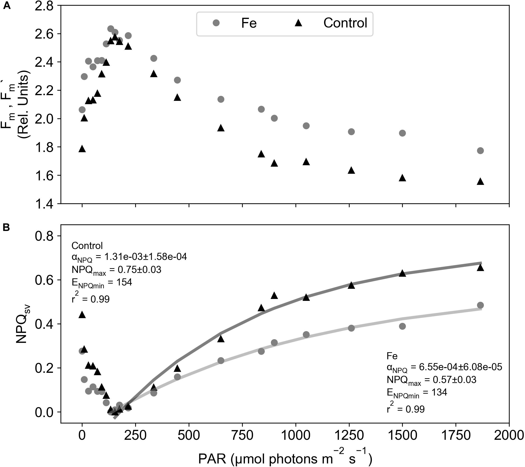
Figure 1. Example chlorophyll fluorescence data from the iron and control treatments of nutrient addition incubation experiment 2 measured at 120 h from Ryan-Keogh et al. (2018a, b); (A) Maximum fluorescence in the dark (Fm) and under actinic light (Fm’), (B) non-photochemical quenching (NPQsv) and (C) NPQsv corrected for ENPQmin fitted with the Platt et al. (1980) model.
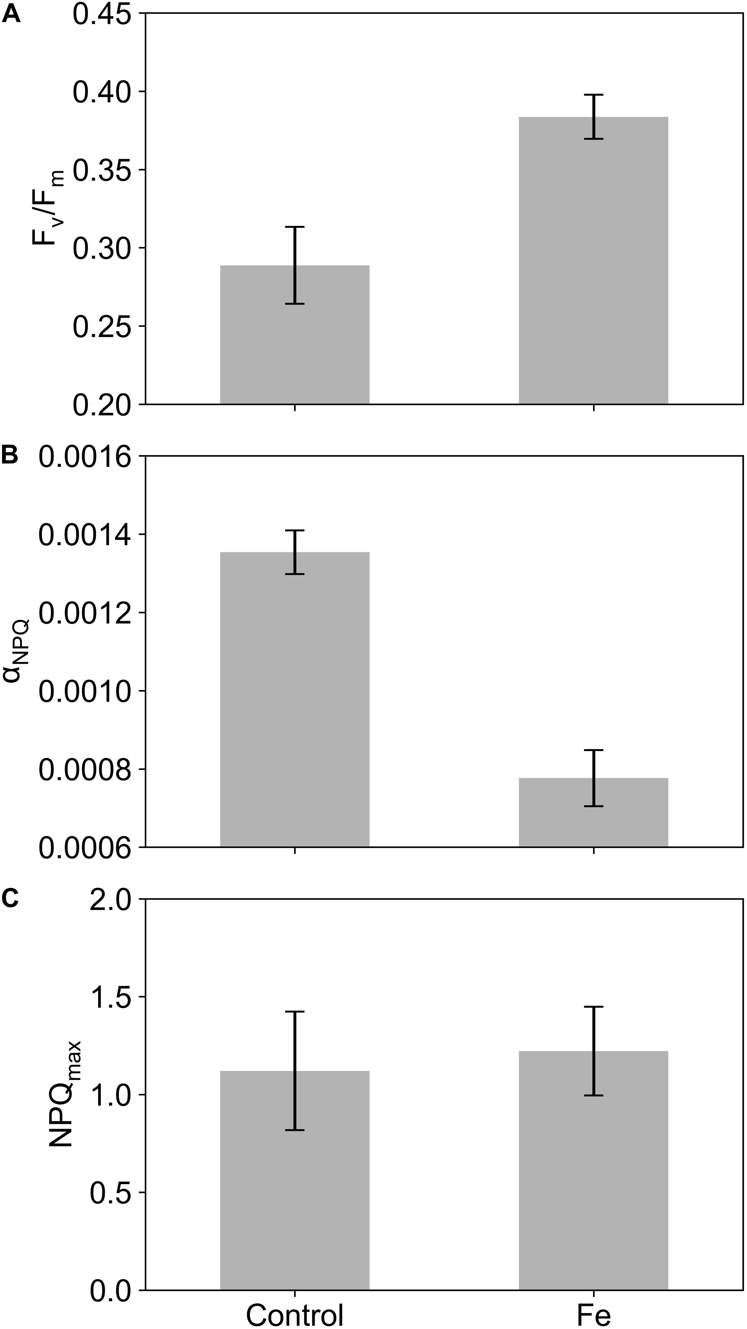
Figure 2. The mean and standard errors of (A) Fv/Fm, (B) αNPQ, and (C) the maximum NPQ value (NPQmax) derived from Platt et al. (1980) from the control and iron addition (Fe) treatments of the nutrient addition incubation experiments, excluding measurements after 120 h (n = 8).
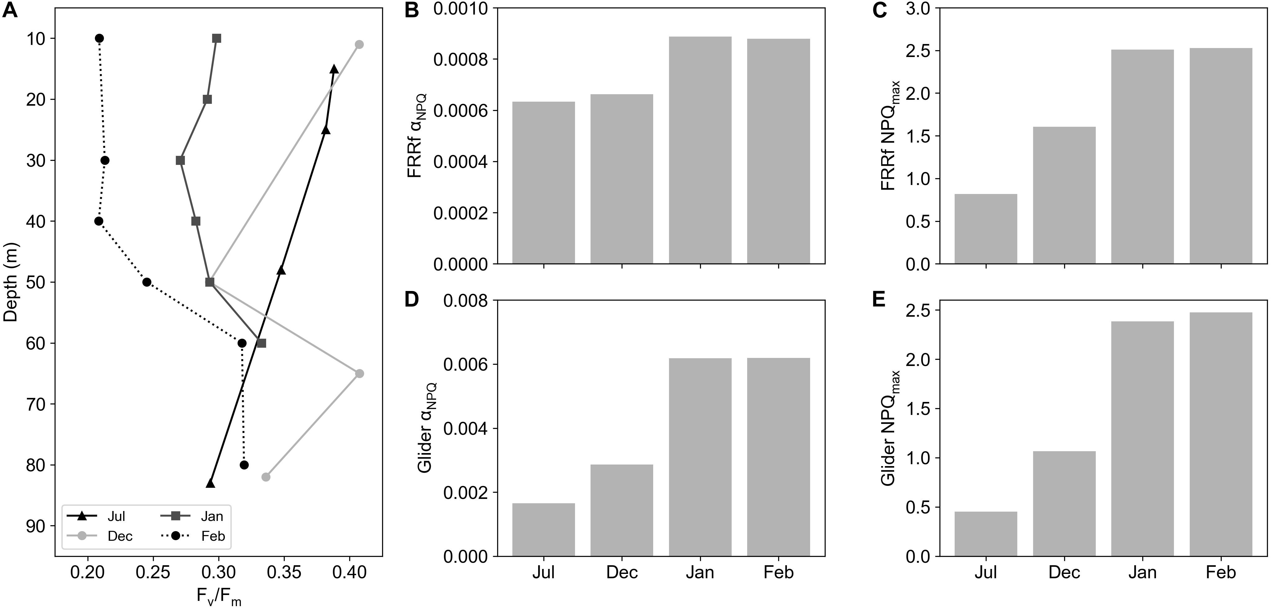
Figure 3. (A) CTD depth profile of Fv/Fm for July, December, January, and February in the Sub-Antarctic Zone. Bar plots of (B) FRRf derived αNPQ, (C) FRRf derived NPQmax, (D) Glider derived αNPQ and (E) Glider derived NPQmax values from surface CTD FLC samples and coincident Glider profiles in July, December, January, and February.
A seasonal signal was evident within NPQGlider, increasing from low values in late July to high values in February (Figure 4). This NPQGlider variability appears to be linked to changes in the MLD (Figure 4A) and increases in surface PAR (Figure 4B). The initial ramp in NPQGlider (e.g., increase in surface NPQGlider from ∼0.3 to ∼3) is coincident with an increase in surface PAR from ∼400 μmol photons m–2 s–1 in late July to ∼800 μmol photons m–2 s–1 in November. PAR beyond November levels out for the remainder of the time series (oscillating around ∼700 μmol photons m–2 s–1) while NPQGlider (surface and mean in MLD) displays large excursions that appear to be linked to variability in the MLD, suggesting a possible switch in the dominant control. Indeed, mean NPQGlider in the MLD remains similar to the mean NPQGlider in the euphotic zone from late July to October (Figure 4B), following which it begins to deviate with increases that are linked to shoaling events in December and January. This same pattern is evident in surface NPQGlider, where a significant positive relationship was observed with surface PAR (Supplementary Figure S3a: r = 0.65, p < 0.05) and a significant negative relationship with MLD (Supplementary Figure S3b: r = −0.82, p < 0.05). These results suggest that both drivers (PAR and MLD) act to increase NPQ, where increased PAR increases phytoplankton light stress, and shoaling events of the MLD increase both light and nutrient stress. By accounting for the effects of light on NPQGlider the remaining variability in NPQGlider across the season can be assumed to be driven primarily by nutrient stress, and secondarily by changes in community structure. However, previous studies have shown that the community structure remained dominated by Haptophytes (>40% of total chlorophyll) throughout winter and summer (Ryan-Keogh et al., 2018a, b). Therefore, we can assume that the majority of variability observed in NPQGlider is driven by iron and light.
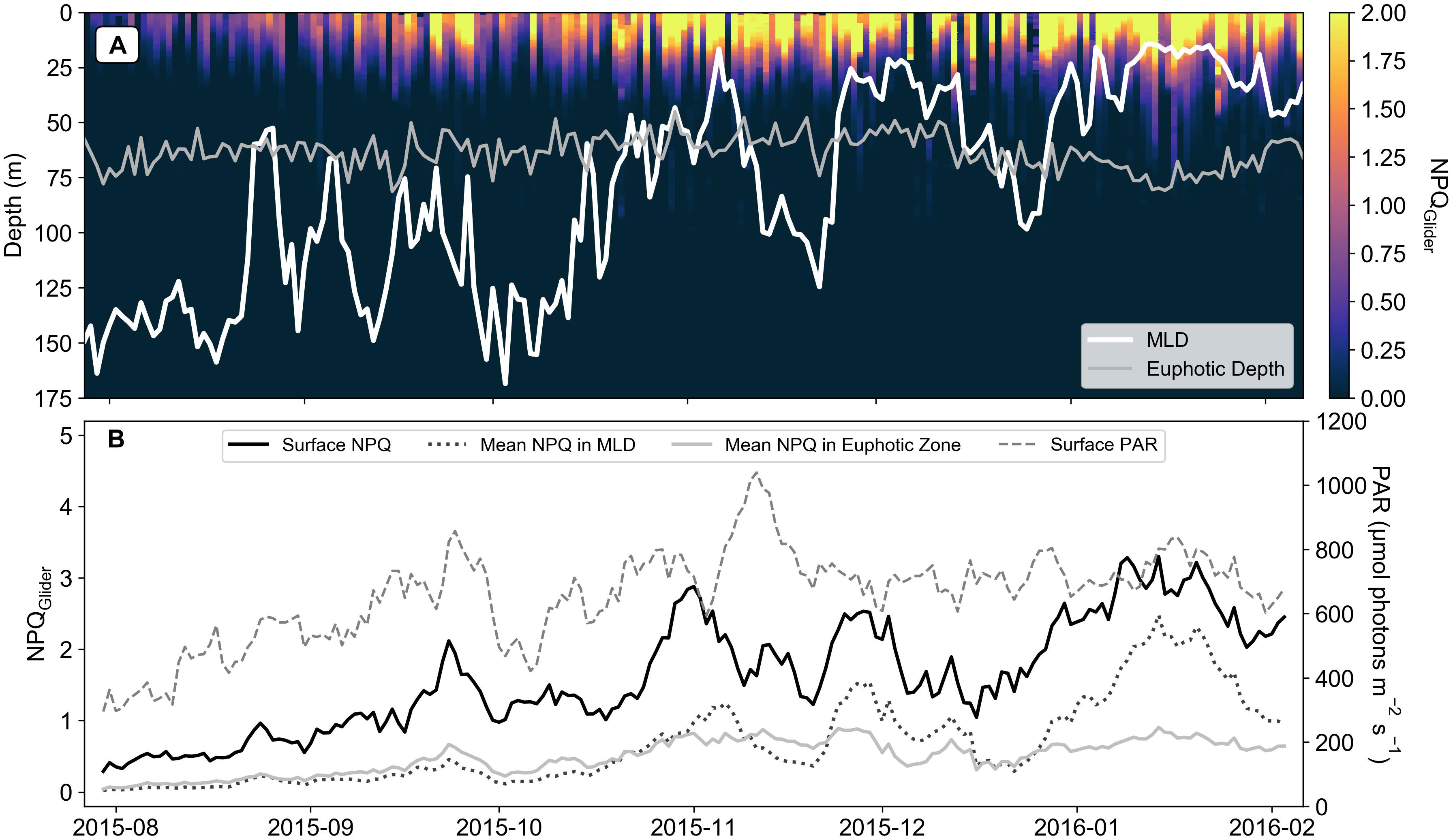
Figure 4. (A) Section of glider derived NPQ (NPQGlider), with the daily mean mixed layer depth (MLD) and euphotic depth (n = 195). (B) A 7-day rolling mean of Surface NPQGlider, mean NPQGlider in MLD, mean NPQGlider in the euphotic zone and surface PAR (μmol photons m– 2 s– 1) for the glider time series.
The depth profile of NPQGlider (Figure 5A) reveals high values in the surface that decrease with depth, similar in shape to the PAR profile (Figure 5B). Moreover, the extent and shape of these profiles is markedly different between winter and summer. By plotting NPQGlider against its relative in situ PAR (Figure 5C) we were able derive the light limited slope of NPQ (αNPQ). This was however not always possible and on six occasions a curve could not be fitted as the daily mean in NPQGlider was zero, in which case the curves were excluded from the analysis. Further quality control (QC) was applied to the data utilizing r2, which ranged from 0.11 to 0.99, with mean and median values of 0.91 and 0.95 respectively. If the r2 value of a fit was less than the total deployment mean r2, the curve was excluded. This QC step resulted in the exclusion of an additional 17 curves, while a total of 172 curves met all QC procedures and were retained. A time series of αNPQ for the glider deployment is plotted in Figure 6A. Between late July and November, before we see the first major deviation between the mean NPQGlider in the MLD and mean NPQGlider in the euphotic zone (Figure 4B), αNPQ increased from a minimum value of 1.65 × 10⁻³ to a maximum value of 1.54 × 10⁻² (Figure 6A and Supplementary Figure S4a), with an interquartile range (IQR) of 3.02 × 10⁻³. After November there is a ∼24% increase in the mean and standard deviation of αNPQ, and this increase in variability can also be seen with a greater standard deviation and range in NPQmax, the maximum NPQGlider value (Supplementary Figure S4b).
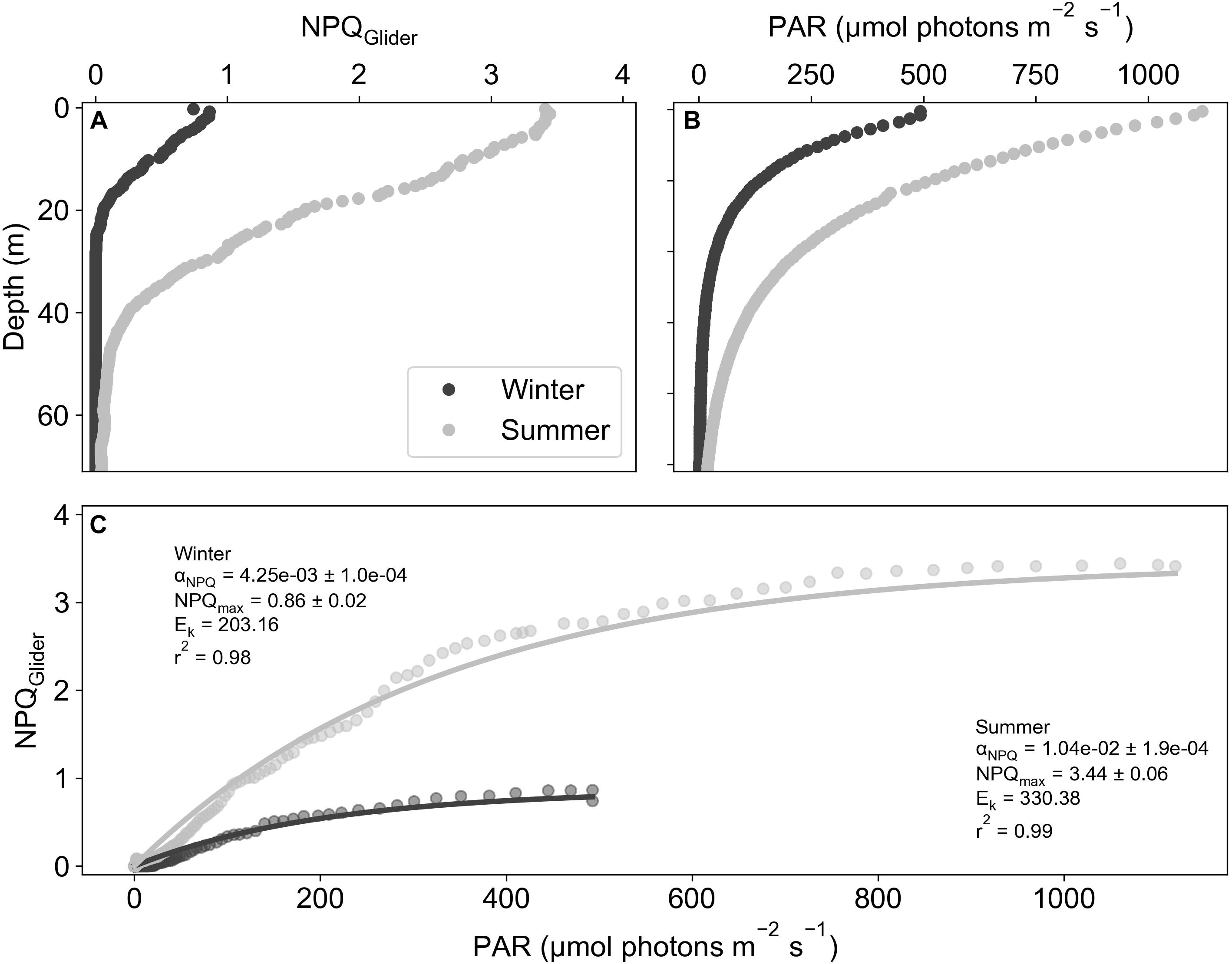
Figure 5. Example depth profiles from glider dives on 13/08/2015 (winter) and 05/01/2016 (summer) of (A) NPQGlider and (B) PAR (μmol photons m– 2 s– 1). (C) Example NPQGlider versus PAR curves for both winter and summer.
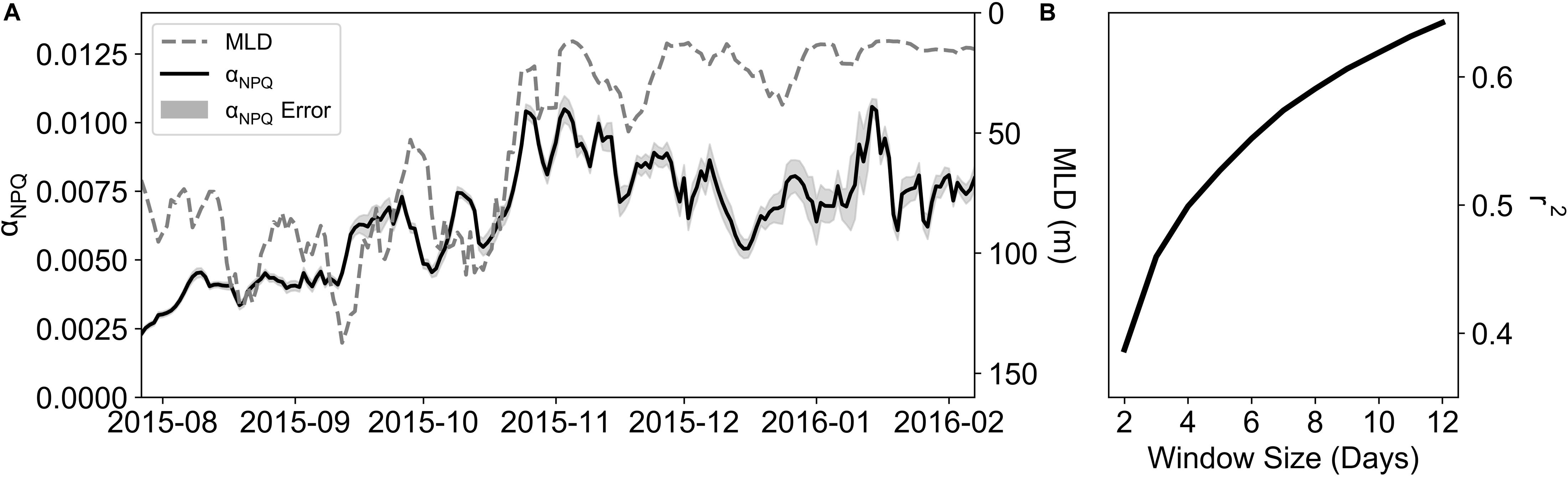
Figure 6. (A) A time-series of a 5-day rolling mean of αNPQ and MLD (m). (B) Correlation coefficients of rolling averages of αNPQ and MLD using different time windows (days).
To estimate the degree to which variability in αNPQ could be linked to nutrient limitation, its relationship to the MLD was examined, where the MLD was used as a proxy for mixing (Fauchereau et al., 2011). αNPQ and MLD (Figure 6A) show similar patterns with time, with increasing αNPQ associated with shallower MLDs. However, no relationship was found between daily changes in MLD and αNPQ (Supplementary Figure S5), which could be linked to the different time scales of variability in physical and biological processes. To examine this further, a series of rolling means of both αNPQ and MLD were created on timescales of 2 to 12 days matching the synoptic variability of storms for this region (Little et al., 2018). Results revealed a high degree of correlation between them with increasing correlation coefficients (r2; Figure 6B) as you increase the time window (r2 = 0.6 for a 10-day window) with 39 to 62% of the variability in αNPQ being explained by MLD on 2 to 10 day time scales.
Discussion
Autonomous platforms, such as buoyancy gliders, can provide unprecedented spatial and temporal coverage of oceanic systems addressing the space-time gaps in observations needed to validate Earth system models. Buoyancy gliders have been successfully deployed in the Atlantic Southern Ocean SAZ under SOSCEx (Swart et al., 2012) to assess the seasonal cycle in this climatically important region (Takahashi et al., 2009; Le Quéré et al., 2013; Frölicher et al., 2014). The seasonal cycle determines environmental variability in light, nutrients and grazing pressure, and as such ascribes the growing conditions that phytoplankton are exposed to over an annual cycle. The seasonal cycle is also the mode of variability that couples the physical mechanisms of climate forcing to the ecosystem response in terms of production, diversity and carbon export (Monteiro et al., 2011). Results from these SAZ glider deployments have been used to examine how variability in physical forcing mechanisms characterize the seasonal cycle of phytoplankton biomass (Swart et al., 2015), to ascertain the role of submesoscale wind-front interactions on driving seasonal restratification (du Plessis et al., 2019), to determine the dominant temporal and spatial scales of variability (Little et al., 2018), to estimate bloom phenology and net community production (Thomalla et al., 2015) and to shed light on the seasonal depletion of dissolved iron reservoirs (Mtshali et al., 2019). The advantages that glider platforms provide (in particular through their high resolution and extended temporal coverage) is clear, however, no studies to date have been able to use these platforms for physiological measurements. Arguably, the most important physiological proxy in large areas of the world’s Ocean, and especially the Southern Ocean, is the response of phytoplankton to iron limitation. This substantiates the appeal for deriving an iron limitation proxy from chlorophyll fluorescence as measured by standard fluorometers on glider platforms.
Here, we develop a method that uses the degree of quenching as a proxy for NPQ similar to that proposed by Schallenberg et al. (2020). In their study, they showed that changes in Fv/Fm in response to iron addition correlated well with NPQsv estimated at a set light level (1000 μmol photons m–2 s–1), such that NPQsv estimated from standard fluorometers could be used as a physiological indicator for iron limitation. However, NPQ is known to increase significantly under saturating light conditions (Schuback et al., 2016) as well as under iron limiting conditions (Schuback et al., 2015; Schuback and Tortell, 2019) making it challenging to separate out one driver from the other. We instead consider the slope of NPQ in relation to in situ light availability, which effectively removes light as a possible driver of variability and instead generates a physiological indicator that is more sensitive to iron limiting growth conditions. To this end, a series of nutrient addition incubation experiments were performed at the same location as the glider deployment on three occasions spanning early to late summer. Concurrent measurements of Fv/Fm and NPQ from FRRf reveal distinct differences in the relationship between NPQ and light in iron addition versus control treatments (Figure 1). By iteratively fitting the model of Platt et al. (1980), key parameters of the relationship between NPQsv and light can be derived (αNPQ and NPQmax). Significant differences were observed between Fv/Fm and αNPQ between the iron and control treatments (Figures 2A,B), highlighting their usefulness as potential proxies for iron limitation. Significant differences were however not apparent for either NPQsv or NPQmax (Figures 2C,D). Since NPQ is affected by both iron and light, these results further advocate for the use of αNPQ as a more reliable proxy for iron limitation. Similar results were found in Fv/Fm data collected from CTD profiles at the same location (Figure 3A), which decreased as the season progressed, indicative of a response to seasonal iron limitation as proposed by Ryan-Keogh et al. (2018b). FLC measurements from the CTD surface samples similarly showed the seasonal progression of in situ changes in NPQ with low αNPQ (Figure 3B) in winter and early summer (July-December) increasing in mid to late summer (January-February) when iron is considered limiting. Unlike in the iron addition incubations however, NPQ also appeared to respond to iron availability with NPQmax (Figure 3C) and NPQsv at 1049 μmol photons m–2 s–1 (Figure 3D) both showing a seasonal increase from late July to December. These results demonstrate how NPQsv can indeed be used as a proxy for iron limitation, however light is simultaneously influencing the variable, driving much lower NPQsv in late July when light is limiting (relative to αNPQ for the same time of year).
The lack of a significant change in Fv/Fm between late July (0.36 ± 0.04) and December (0.35 ± 0.03) combined with the lack of response to iron addition in experiment 1 from Ryan-Keogh et al. (2018b) suggest that during this period (i.e., winter and early summer) iron is not limiting. This is similarly reflected in the lack of change in αNPQ between winter (July) and early summer (December). The increase in NPQ values (from late July to December) is thus likely driven by an increase in available PAR (Figure 4B), while beyond December the changes in NPQ are likely driven by both iron and light. These results suggest that αNPQ variability, which accounts for the effect of light availability, provides a more suitable proxy for iron limitation, bearing in mind that community structure will also play a role. However, this was not the case for this study where the community structure remained relatively unchanged (>40% Haptophytes) throughout the growing season (Ryan-Keogh et al., 2018a, b).
Determining this proxy from gliders however requires measurements of NPQ in the absence of active chlorophyll fluorescence from a FRRf (or similar). Instead, the ratio of quenched fluorescence to quenching corrected fluorescence (Thomalla et al., 2018) was used to derive a proxy for NPQ. NPQGlider showed a clear seasonal cycle, increasing as the growing season progressed (Figure 4A), consistent with increased light availability (Figure 4B), a shoaling of the MLD (Figure 4A) and anticipated iron limitation (Ryan-Keogh et al., 2018b; Mtshali et al., 2019). Since both incident PAR and MLD determine the extent of light exposure to phytoplankton, it is not surprising that a strong seasonal relationship is observed with the initial ramp in NPQGlider. From November onwards however, NPQGlider remained variable despite similar levels of PAR, which oscillates around ∼700 μmol photons m–2 s–1 suggesting a switch in the dominant control of NPQGlider from surface PAR variability to MLD variability (which influences water column integrated light as well as nutrient availability). Surface NPQGlider showed both a significant positive relationship with surface PAR (Supplementary Figure S3a) and a significant negative relationship with MLD (Supplementary Figure S3b), as both of these drivers act to increase NPQGlider, through an increase in light and nutrient stress. If the specific effect of light can be accounted for, then the remaining variability in NPQGlider will primarily be driven by either nutrient stress or community structure. One way to account for in situ light is to utilize the relationship between the PAR and NPQGlider profiles (Figure 5), which reveals a markedly similar shape to that of NPQsv derived from a FLC. By applying the same analytical approach as the FLC data, we were able to fit the model of Platt et al. (1980) to derive the same NPQ parameters (Glider αNPQ and Glider NPQmax), with variation in αNPQ having already been established from in situ data as a suitable proxy for iron limitation. As a further test of the robustness of our method, glider derived estimates of αNPQ and NPQmax (daily means) were compared with independent measurements of αNPQ and NPQmax from FRRf (measured at the same station on the same day but an instantaneous measurement rather than a daily mean). Bearing in mind that the absolute values are not comparable, similar trends should at least be evident in both measurements. This is the case for both glider and FRRf derived αNPQ (Figures 3B,D) and NPQmax (Figures 3C,E) which increased across the growing season with lower values in late July and December compared to January and February when iron was considered limiting.
A closer look at the time series of glider derived αNPQ showed the greatest increase in variability after November, with a 24% increase in the mean and standard deviation. A similar increase in variability is also evident within NPQmax (Supplementary Figure S4b). The transition period for the different modes of variability appears to coincide with the date of mixed layer restratification (26th November) determined for the same glider time series by du Plessis et al. (2019) as the date when mean stratification above the winter mixed layer persistently increases and positive net heat flux takes over as the dominant driver of stratification (as opposed to transient stratification events associated with submesoscale processes). Similarly, a study by Swart et al. (2015) from a different glider time series but also in the Atlantic SAZ identified the 28th of November as the date which separated their time series into spring and summer based on contrasting characteristics of upper ocean physics and chlorophyll. In their study, the summer period was characterized by enhanced stratification that prevented extensive deepening of the MLD, which nonetheless remained highly variable at subseasonal time scales (Swart et al., 2015) driven by wind stress from synoptic storm events (4–9 days). They proposed that the observed MLD variability was responsible for regulating light and iron supply to surface waters at appropriate time scales for phytoplankton growth, thereby sustaining the SAZ phytoplankton bloom into late summer. Since then, there have been a number of additional studies which suggest that in addition to deep winter entrainment and recycling (Tagliabue et al., 2014), intermittent storm-driven mixing may play an important role in extending the duration of summertime production in the SAZ and other regions through intraseasonal entrainment of iron from a subsurface reservoir beneath the productive layer (Smith et al., 2011; Carranza and Gille, 2015; Thomalla et al., 2015; Nicholson et al., 2016, 2019; Mtshali et al., 2019). As an example, Mtshali et al. (2019) examined the seasonal evolution of dissolved iron profiles at a single station in the SAZ to explore different mechanisms driving iron availability (convective mixing, biological consumption, scavenging, recycling, and entrainment). While this study provides useful insight into ecosystem dynamics, the four CTD occupations fail to capture event scale dynamics of how the ecosystem evolves over the growing season. With the use of passive chlorophyll fluorescence on gliders to derive photophysiological indicators of nutrient stress and relief, we can for the first time try to address these questions at the full range of scales appropriate to the dynamics of nutrient supply and demand.
Whilst the MLD does not exhibit particularly large excursions after November (Supplementary Figure S5), this is the period when phytoplankton begin to exhibit signs of nutrient stress (Ryan-Keogh et al., 2018b), there are large decreases in iron availability (Mtshali et al., 2019) and αNPQ is most variable (Supplementary Figure S4). The seasonal relationship between αNPQ and MLD agrees with the notion that as summer progresses there is an increase in nutrient stress and an associated increase in αNPQ (Figure 6A). However, the correlation between MLD and αNPQ was poor (r2 = 0.22; data not shown), potentially driven by several shallow MLDs with a wide range of αNPQ. This finding was not unexpected given the variable response of phytoplankton to changes in the MLD, e.g., dilution (a decrease in biomass with a deepening of the MLD), growth (an increase in biomass with both a deepening of the MLD in response to nutrient entrainment and a shoaling of the MLD in response to increased light availability) (Fauchereau et al., 2011), and both nutrient and light stress associated with shallow MLDs. Similarly, weak linear correlations were observed between physical variables and chlorophyll by Swart et al. (2015) and Little et al. (2018). However, a comparison by Little et al. (2018) of the dominant modes of variability in wind stress, MLD, SST and chlorophyll showed that in spring all variables displayed similar scales of variability (2, 8, and 10 days) with fine scales (<10 days) accounting for 97% of the chlorophyll variability. In summer, a larger scale signal dominated chlorophyll (27 days, 54%) with fine scales (2, 4, and 9 days) still accounting for a significant amount of the chlorophyll variability (27%) comparable to fine scale (<10 days) variability in the physical variables (wind stress, MLD and salinity) from synoptic storm events (Carranza and Gille, 2015; Swart et al., 2015), which have been linked to the entrainment of subsurface iron (Nicholson et al., 2016).
Given a better understanding of the dominant scales of variability, a series of correlations were performed between αNPQ and MLD using rolling means of time scales ranging from 2 to 12 days and indeed, correlation coefficients increased from 0.39 to 0.64 (Figure 6B). EMD analysis (as per Little et al., 2018) similarly confirmed the dominance of fine scale variability (Supplementary Table S1), with 46–53% of αNPQ variability in summer occurring on time scales of less than 7 days (with 48–66% in spring). Whilst the correlation coefficients continued to increase to a maximum of 0.79 (data not shown), they do so close to a monthly time scale (>25 days) and may be representative of other physical processes at play. Moreover, the EMD analysis of αNPQ found that at these time scales none of the IMFs were significant (p > 0.01). Given that the dominant scales of variability of summer αNPQ are coincident with the physical drivers of MLD variability and that there is a strong correlation between αNPQ and MLD at a ∼10 day window, we can suggest that synoptic storms which pass through the SAZ alter the MLD which in turn alters the nutrient supply to phytoplankton driving the observed variability in αNPQ; i.e., event-scale entrainment of iron is taking place and likely contributing to the sustained summer blooms characteristic of the SAZ.
Conclusion
Whilst gliders have provided extensive in depth understanding of fine scale physical dynamics and phytoplankton production in the SAZ (Swart et al., 2015; du Plessis et al., 2017, 2019; Little et al., 2018) and other regions (Briggs et al., 2011; Alkire et al., 2014; Biddle et al., 2015; Erickson et al., 2016; Bol et al., 2018; Queste et al., 2018; Viglione et al., 2018), our ability to attain a similar degree of resolution from physiological applications is somewhat lacking. This study suggests that if you can correct fluorescence quenching, you can use the degree of quenching to estimate NPQ which when plotted against available light (i.e., derive the slope) can provide physiological information of phytoplankton (i.e., iron stress). This novel method is particularly suited to autonomous platforms such as floats and buoyancy gliders, whose use in open ocean oceanography is seeing a rapid increase. Application of this method to our glider deployment in the Atlantic SAZ spanning winter to late summer shows a seasonal increase in αNPQ, a shoaling of the MLD and seasonal iron limitation (Ryan-Keogh et al., 2018b; Mtshali et al., 2019). The dominant scales of variability of αNPQ (with the seasonal signal removed) are consistent with fine scale (<10 day) variability in the physical drivers of wind (Little et al., 2018) and MLD and a significant positive relationship (r2 = 0.62) is observed between αNPQ and MLD at a ∼10 day window. These results emphasize the important role of fine scale dynamics linked to synoptic storms in driving iron supply to the SAZ, particularly in summer when this micronutrient is especially limiting. Application of this methodology to different biogeochemical regimes will begin to shed light on the seasonal dynamics of both iron limitation and iron co-limitation, with downstream implications for understanding changes in chlorophyll biomass and primary production at the required scales necessary for validation and improved parameterisation of Earth system models. We are cognisant of the fact that this approach has been developed from the results of iron incubation experiments in the Atlantic SAZ and would thus benefit from additional experiments in a variety of ocean regions to warrant a more confident global application. As such, we invite the fluorescence community to perform similar experiments to confirm that significant differences are observed between Fv/Fm and αNPQ between nutrient addition and control treatments.
Data Availability Statement
Glider data is available at ftp://socco.chpc.ac.za/GliderTools/SOSCEx3. Experimental and CTD data are at ftp://socco.chpc.ac.za/RyanKeogh_Thomalla_Glider_2020/.
Author Contributions
TR-K and ST designed the study, analyzed the data, and wrote the manuscript.
Conflict of Interest
The authors declare that the research was conducted in the absence of any commercial or financial relationships that could be construed as a potential conflict of interest.
The reviewer WS declared a past co-authorship with one of the authors TR-K to the handling Editor.
Funding
This work was undertaken through the CSIR’s Southern Ocean Carbon and Climate Observatory (SOCCO) Programme (http://socco.org.za) and supported by CSIR’s Parliamentary Grant funding (SNA2011112600001) and NRF SANAP grants (SNA2011120800004 and SNA14071475720).
Acknowledgments
We thank the South African National Antarctic Programme (SANAP) and the captain, officers, and crew of the SA Agulhas II for their professional support throughout the cruise. We are thankful for the professional service delivered by the engineers and glider pilots from Sea Technology Services.
Supplementary Material
The Supplementary Material for this article can be found online at: https://www.frontiersin.org/articles/10.3389/fmars.2020.00275/full#supplementary-material
References
Abbott, M. R., Richerson, P. J., and Powell, T. M. (1982). In situ response of phytoplankton fluorescence to rapid variations in light. Limnol. Oceanogr. 27, 218–225. doi: 10.4319/lo.1982.27.2.0218
Alderkamp, A. C., Kulk, G., Buma, A. G. J., Visser, R. J. W., Van Dijken, G. L., Mills, M. M., et al. (2012). The effect of iron limitation on the photophysiology of phaeocystis antarctica (prymnesiophyceae) and fragilariopsis cylindrus (bacillariophyceae) under dynamic irradiance. J. Phycol. 48, 45–59. doi: 10.1111/j.1529-8817.2011.01098.x
Alkire, M. B., Lee, C., D’Asaro, E., Perry, M. J., Briggs, N., Cetiniæ, I., et al. (2014). Net community production and export from Seaglider measurements in the North Atlantic after the spring bloom. J. Geophys. Res. Oceans 119, 6121–6139. doi: 10.1002/2014jc010105
Behrenfeld, M. J., Westberry, T. K., Boss, E. S., O’Malley, R. T., Siegel, D. A., Wiggert, J. D., et al. (2009). Satellite-detected fluorescence reveals global physiology of ocean phytoplankton. Biogeosciences 6, 779–794. doi: 10.5194/bg-6-779-2009
Biddle, L. C., Kaiser, J., Heywood, K. J., Thompson, A. F., and Jenkins, A. (2015). Ocean glider observations of iceberg-enhanced biological production in the northwestern Weddell Sea. Geophys. Res. Lett. 42, 459–465. doi: 10.1002/2014gl062850
Biermann, L., Guinet, C., Bester, M., Brierley, A., and Boehme, L. (2015). An alternative method for correcting fluorescence quenching. Ocean Sci. 11, 83–91. doi: 10.5194/os-11-83-2015
Bilger, W., and Björkman, O. (1990). Role of the xanthophyll cycle in photoprotection elucidated by measurements of light-induced absorbance changes, fluorescence and photosynthesis in leaves of Hedera canariensis. Photosynth. Res. 25, 173–186. doi: 10.1007/BF00033159
Bol, R., Henson, S. A., Rumyantseva, A., and Briggs, N. (2018). High-frequency variability of small-particle carbon export flux in the northeast Atlantic. Glob. Biogeochem. Cycles 32, 1803–1814. doi: 10.1029/2018gb005963
Boyd, P. W., Jickells, T., Law, C. S., Blain, S., Boyle, E. A., Buesseler, K. O., et al. (2007). Mesoscale iron enrichment experiments 1993-2005: synthesis and future directions. Science 315, 612–617. doi: 10.1126/science.1131669
Bricaud, A., and Stramski, D. (1990). Spectral absorption coefficients of living phytoplankton and nonalgal biogenous matter: a comparison between the Peru upwelling area and the Sargasso Sea. Limnol. Oceanogr. 35, 562–582. doi: 10.4319/lo.1990.35.3.0562
Briggs, N., Perry, M. J., Cetiniæ, I., Lee, C., D’Asaro, E., Gray, A. M., et al. (2011). High-resolution observations of aggregate flux during a sub-polar North Atlantic spring bloom. Deep Sea Res. Part I Oceanogr. Res. Pap. 58, 1031–1039. doi: 10.1016/j.dsr.2011.07.007
Browning, T. J., Bouman, H. A., and Moore, C. M. (2014). Satellite detected fluorescence: decoupling nonphotochemical quenching form iron stress signals in the South Atlantic and Southern Ocean. Glob. Biogeochem. Cycles 28, 510–524. doi: 10.1002/2013gb004773
Carranza, M. M., and Gille, S. T. (2015). Southern Ocean wind-driven entrainment enhances satellite chlorophyll-a through the summer. J. Geophys. Res. Oceans 120, 304–323. doi: 10.1002/2014jc010203
Coleman, T., and Li, Y. (1996). An interior trust region approach for nonlinear minimization subject to bounds. SIAM J. Optim. 6, 418–445. doi: 10.1137/0806023
Coleman, T. F., and Li, Y. (1994). On the convergence of interior-reflective Newton methods for nonlinear minimization subject to bounds. Math. Program. 67, 189–224. doi: 10.1007/bf01582221
Constable, A. J., Costa, D. P., Schofield, O., Newman, L., Urban, E. R., Fulton, E. A., et al. (2016). Developing priority variables (“ecosystem Essential Ocean Variables” — eEOVs) for observing dynamics and change in Southern Ocean ecosystems. J. Mar. Syst. 161, 26–41. doi: 10.1016/j.jmarsys.2016.05.003
Cullen, J. J. (1982). The deep chlorophyll maximum: comparing vertical profiles of chlorophyll a. Can. J. Fish. Aquat. Sci. 39, 791–803. doi: 10.1139/f82-108
Cullen, J. J., and Davis, R. F. (2003). The blank can make a big difference in oceanographic measurements. Limnol. Oceanogr. Bull. 12, 29–35. doi: 10.1002/lob.200312229
de Boyer Montégut, C., Madec, G., Fischer, A. S., Lazar, A., and Iudicone, D. (2004). Mixed layer depth over the global ocean: an examination of profile data and a profile-based climatology. J. Geophys. Res. Oceans 109:C12003. doi: 10.1029/2004JC002378
Demmig-Adams, B., and Adams, W. W. (1996). Xanthophyll cycle and light stress in nature: uniform response to excess direct sunlight among higher plant species. Planta 198, 460–470. doi: 10.1007/bf00620064
du Plessis, M., Swart, S., Ansorge, I. J., and Mahadevan, A. (2017). Submesoscale processes promote seasonal restratification in the Subantarctic Ocean. J. Geophys. Res. Oceans 122, 2960–2975. doi: 10.1002/2016jc012494
du Plessis, M., Swart, S., Ansorge, I. J., Mahadevan, A., and Thompson, A. F. (2019). Southern ocean seasonal restratification delayed by Submesoscale wind–front interactions. J. Phys. Oceanogr. 49, 1035–1053. doi: 10.1175/jpo-d-18-0136.1
Erickson, Z. K., Thompson, A. F., Cassar, N., Sprintall, J., and Mazloff, M. R. (2016). An advective mechanism for deep chlorophyll maxima formation in southern Drake Passage. Geophys. Res. Lett. 43, 10,846–10,855. doi: 10.1002/2016GL070565
Falkowski, P. G., and Kolber, Z. (1995). Variations in chlorophyll fluorescence yields in phytoplankton in the world oceans. Aust. J. Plant Physiol. 22, 341–355. doi: 10.1071/PP9950341
Falkowski, P. G., and Raven, J. A. (2007). Aquatic Photosynthesis, 2nd Edn. Princeton, NJ: Princeton University Press.
Fauchereau, N., Tagliabue, A., Bopp, L., and Monteiro, P. M. S. (2011). The response of phytoplankton biomass to transient mixing events in the Southern Ocean. Geophys. Res. Lett. 38:L17601. doi: 10.1029/2011GL048498
Frölicher, T. L., Sarmiento, J. L., Paynter, D. J., Dunne, J. P., Krasting, J. P., and Winton, M. (2014). Dominance of the Southern ocean in anthropogenic carbon and heat uptake in CMIP5 models. J. Clim. 28, 862–886. doi: 10.1175/jcli-d-14-00117.1
Geider, R. J. (1993). Quantitative phytoplankton physiology: implications for primary production and phytoplankton growth. ICES Mar. Sci. Symp. 197, 52–62.
Gregor, L., Ryan-Keogh, T. J., Nicholson, S.-A., du Plessis, M. D., Giddy, I., and Swart, S. (2019). GliderTools: a python toolbox for processing underwater glider data. Front. Mar. Sci. 6:738. doi: 10.3389/fmars.2019.00738
Hemsley, V. S., Smyth, T. J., Martin, A. P., Frajka-Williams, E., Thompson, A. F., Damerell, G., et al. (2015). Estimating oceanic primary production using vertical irradiance and chlorophyll profiles from ocean gliders in the north Atlantic. Environ. Sci. Technol. 49, 11612–11621. doi: 10.1021/acs.est.5b00608
Hiscock, M. R., Lance, V. P., Apprill, A. M., Bidigare, R. R., Johnson, Z. I., Mitchell, B. G., et al. (2008). Photosynthetic maximum quantum yield increases are an essential component of the Southern Ocean phytoplankton response to iron. Proc. Natl. Acad. Sci. U.S.A. 105, 4775–4780. doi: 10.1073/pnas.0705006105
Hughes, D. J., Campbell, D. A., Doblin, M. A., Kromkamp, J. C., Lawrenz, E., Moore, C. M., et al. (2018). Roadmaps and detours: active chlorophyll- a assessments of primary productivity across marine and freshwater systems. Environ. Sci. Technol. 52, 12039–12054. doi: 10.1021/acs.est.8b03488
IOCCG Protocol Series (2018). Inherent Optical Property Measurements and Protocols: Absorption Coefficient, eds A. R. Neely and A. Mannino (Dartmouth: IOCCG).
Kiefer, D. A. (1973). Fluorescence properties of natural phytoplankton populations. Mar. Biol. 22, 263–269. doi: 10.1007/bf00389180
Kolber, Z. S., Prášil, O., and Falkowski, P. G. (1998). Measurements of variable chlorophyll fluorescence using fast repetition rate techniques: defining methodology and experimental protocols. Biochim. Biophys. Acta 1367, 88–106. doi: 10.1016/s0005-2728(98)00135-2
Kropuenske, L. R., Mills, M. M., van Dijken, G. L., Bailey, S., Robinson, D. H., Welschmeyer, N. A., et al. (2009). Photophysiology in two major Southern Ocean phytoplankton taxa: photoprotection in phaeocystis antarctica and fragilariopsis cylindrus. Limnol. Oceanogr. 54, 1176–1196. doi: 10.4319/lo.2009.54.4.1176
Le Quéré, C., Andres, R. J., Boden, T., Conway, T., Houghton, R. A., House, J. I., et al. (2013). The global carbon budget 1959–2011. Earth Syst. Sci. Data 5, 165–185.
Little, H. J., Vichi, M., Thomalla, S. J., and Swart, S. (2018). Spatial and temporal scales of chlorophyll variability using high-resolution glider data. J. Mar. Syst. 187, 1–12. doi: 10.1016/j.jmarsys.2018.06.011
Lorenzen, C. J. (1966). A method for the continuous measurement of in vivo chlorophyll concentrations. Deep Sea Res. Oceanogr. Abstr. 13, 223–277.
Milligan, A. J., Aparicio, U. A., and Behrenfeld, M. J. (2012). Fluorescence and nonphotochemical quenching responses to simulated vertical mixing in the marine diatom Thalassiosira weissflogii. Mar. Ecol. Prog. Ser. 448, 67–78. doi: 10.3354/meps09544
Mitchell, B., Kahru, M., Wieland, J., and Stramska, M. (2002). “Determination of spectral absorption coefficients of particles, dissolved material and phytoplankton for discrete water samples,” in Ocean Optics Protocols for Satellite Ocean Color Sensor Validation, eds J. L. Mueller and G. S. Fargion (Greenbelt, MD: NASA Goddard Space Flight Centre), 231–257.
Monteiro, P. M. S., Boyd, P., and Bellerby, R. (2011). Role of the seasonal cycle in coupling climate and carbon cycling in the subantarctic zone. Eos Trans. Am. Geophys. Union 92, 235–236. doi: 10.1029/2011eo280007
Moore, C. M., Mills, M. M., Arrigo, K. R., Berman-Frank, I., Bopp, L., Boyd, P. W., et al. (2013). Processes and patterns of oceanic nutrient limitation. Nat. Geosci. 6, 701–710. doi: 10.1038/ngeo1765
Moore, C. M., Seeyave, S., Hickman, A. E., Allen, J. T., Lucas, M. I., Planquette, H., et al. (2007). Iron-light interactions during the CROZet natural iron bloom and EXport experiment (CROZEX) I: phytoplankton growth and photophysiology. Deep Sea Res. Part II Top. Stud. Oceanogr. 54, 2045–2065. doi: 10.1016/j.dsr2.2007.06.011
Morel, A., Claustre, H., Antoine, D., and Gentili, B. (2007). Natural variability of bio-optical properties in Case 1 waters: attenuation and reflectance within the visible and near-UV spectral domains, as observed in South Pacific and Mediterranean waters. Biogeosciences 4, 913–925. doi: 10.5194/bg-4-913-2007
Mtshali, T. N., van Horsten, N. R., Thomalla, S. J., Ryan-Keogh, T. J., Nicholson, S.-A., Roychoudhury, A. N., et al. (2019). Seasonal depletion of the dissolved iron reservoirs in the sub-Antarctic zone of the southern Atlantic ocean. Geophys. Res. Lett. 46, 4386–4395. doi: 10.1029/2018gl081355
Müller, P., Li, X.-P., and Niyogi, K. K. (2001). Non-photochemical quenching. A response to excess light energy. Plant Physiol. 125, 1558–1566. doi: 10.1104/pp.125.4.1558
Nicholson, S.-A., Lévy, M., Jouanno, J., Capet, X., Swart, S., and Monteiro, P. M. S. (2019). Iron supply pathways between the surface and subsurface waters of the Southern Ocean: from winter entrainment to summer storms. Geophys. Res. Lett. 46, 14567–14575. doi: 10.1029/2019GL084657
Nicholson, S.-A., Lévy, M., Llort, J., Swart, S., and Monteiro, P. M. S. (2016). Investigation into the impact of storms on sustaining summer primary productivity in the Sub-Antarctic Ocean. Geophys. Res. Lett. 43, 9192–9199. doi: 10.1002/2016gl069973
O’Malley, R. T., Behrenfeld, M. J., Westberry, T. K., Milligan, A. J., Shang, S., and Yan, J. (2014). Geostationary satellite observations of dynamic phytoplankton photophysiology. Geophys. Res. Lett. 41, 5052–5059. doi: 10.1002/2014gl060246
Owens, T. G., Falkowski, P. G., and Whitledge, T. E. (1980). Diel periodicity in cellular chlorophyll content in marine diatoms. Mar. Biol. 59, 71–77. doi: 10.1007/bf00405456
Platt, T., Gallegos, C. L., and Harrison, W. G. (1980). Photoinhibition of photosynthesis in natural assemblages of marine phytoplankton. J. Mar. Res. 38, 687–701.
Queste, B. Y., Vic, C., Heywood, K. J., and Piontkovski, S. A. (2018). Physical controls on oxygen distribution and denitrification potential in the North West Arabian sea. Geophys. Res. Lett. 45, 4143–4152. doi: 10.1029/2017gl076666
Rato, R. T., Ortigueira, M. D., and Batista, A. G. (2008). On the HHT, its problems, and some solutions. Mech. Syst. Signal Process. 22, 1374–1394. doi: 10.1016/j.ymssp.2007.11.028
Roháček, K. (2002). Chlorophyll fluorescence parameters: the definitions, photosynthetic meaning, and mutual relationships. Photosynthetica 40, 13–29. doi: 10.1023/A:1020125719386
Ryan-Keogh, T. J., and Robinson, C. M. (0000). Phytoplankton photophysiology utilities: tools for the standardisation of processing active chlorophyll fluorescence data. Front. Mar. Sci.
Ryan-Keogh, T. J., Thomalla, S. J., Little, H. J., and Melanson, J. R. (2018a). Seasonal regulation of the coupling between photosynthetic electron transport and carbon fixation in the Southern Ocean. Limnol. Oceanogr. 63, 1856–1876. doi: 10.1002/lno.10812
Ryan-Keogh, T. J., Thomalla, S. J., Mtshali, T. N., van Horsten, N. R., and Little, H. J. (2018b). Seasonal development of iron limitation in the sub-Antarctic zone. Biogeosciences 15, 4647–4660. doi: 10.5194/bg-15-4647-2018
Ryan-Keogh, T. J., Thomalla, S. J., Mtshali, T. N., and Little, H. (2017). Modelled estimates of spatial variability of iron stress in the Atlantic sector of the Southern Ocean. Biogeosciences 14, 3883–3897. doi: 10.5194/bg-14-3883-2017
Sackmann, B. S., Perry, M. J., and Eriksen, C. C. (2008). Fluorescene quenching from Seaglider observations of variability in daytime fluorescence quenching of chlorophyll-a in Northeastern Pacific coastal waters Fluorescence quenching from Seaglider. Biogeosci. Discuss. 5, 2839–2865. doi: 10.5194/bgd-5-2839-2008
Schallenberg, C., Lewis, M. R., Kelley, D. E., and Cullen, J. J. (2008). Inferred influence of nutrient availability on the relationship between Sun-induced chlorophyll fluorescence and incident irradiance in the Bering Sea. J. Geophys. Res. Oceans 113, 1–21. doi: 10.1029/2007JC004355
Schallenberg, C., Strzepek, R. F., Schuback, N., Clementson, L. A., Boyd, P. W., and Trull, T. W. (2020). Diel quenching of Southern Ocean phytoplankton fluorescence is related to iron limitation. Biogeosciences 17, 793–812. doi: 10.5194/bg-17-793-2020
Schuback, N., Flecken, M., Maldonado, M. T., and Tortell, P. D. (2016). Diurnal variation in the coupling of photosynthetic electron transport and carbon fixation in iron-limited phytoplankton in the NE subarctic Pacific. Biogeosciences 13, 1019–1035. doi: 10.5194/bg-13-1019-2016
Schuback, N., Schallenberg, C., Duckham, C., Maldonado, M. T., and Tortell, P. D. (2015). Interacting effects of light and iron availability on the coupling of photosynthetic electron transport and CO2-assimilation in marine phytoplankton. PLoS One 10:e0133235. doi: 10.1371/journal.pone.0133235
Schuback, N., and Tortell, P. D. (2019). Diurnal regulation of photosynthetic light absorption, electron transport and carbon fixation in two contrasting oceanic environments. Biogeosciences 16, 1381–1399. doi: 10.5194/bg-16-1381-2019
Serôdio, J., Cruz, S., Vieira, S., and Brotas, V. (2005). Non-photochemical quenching of chlorophyll fluorescence and operation of the xanthophyll cycle in estuarine microphytobenthos. J. Exp. Mar. Bio. Ecol. 326, 157–169. doi: 10.1016/j.jembe.2005.05.011
Slovacek, R. E., and Hannan, P. J. (1977). In vivo fluorescence determinations of phytoplankton chlorophyll a. Limnol. Oceanogr. 22, 919–925. doi: 10.4319/lo.1977.22.5.0919
Smith, W. O., Asper, V., Tozzi, S., Liu, X., and Stammerjohn, S. E. (2011). Surface layer variability in the Ross Sea, Antarctica as assessed by in situ fluorescence measurements. Prog. Oceanogr. 88, 28–45. doi: 10.1016/j.pocean.2010.08.002
Stomp, M., Huisman, J., Stal, L. J., and Matthijs, H. C. P. (2007a). Colorful niches of phototrophic microorganisms shaped by vibrations of the water molecule. ISME J. 1, 271–282. doi: 10.1038/ismej.2007.59
Stomp, M., Huisman, J., Vörös, L., Pick, F. R., Laamanen, M., Haverkamp, T., et al. (2007b). Colourful coexistence of red and green picocyanobacteria in lakes and seas. Ecol. Lett. 10, 290–298. doi: 10.1111/j.1461-0248.2007.01026.x
Stramski, D., Reynolds, R. A., Kaczmarek, S., Uitz, J., and Zheng, G. (2015). Correction of pathlength amplification in the filter-pad technique for measurements of particulate absorption coefficient in the visible spectral region. Appl. Opt. 54, 6763–6782. doi: 10.1364/AO.54.006763
Swart, S., Chang, N., Fauchereau, N., Joubert, W., Lucas, M., Mtshali, T., et al. (2012). Southern Ocean Seasonal Cycle Experiment 2012: seasonal scale climate and carbon cycle links. S. Afr. J. Sci. 108, 11–13. doi: 10.4102/sajs.v108i3/4.1089
Swart, S., Thomalla, S. J., and Monteiro, P. M. S. (2015). The seasonal cycle of mixed layer dynamics and phytoplankton biomass in the Sub-Antarctic Zone: a high-resolution glider experiment. J. Mar. Syst. 147, 103–115. doi: 10.1016/j.jmarsys.2014.06.002
Tagliabue, A., Sallée, J. B., Bowie, A. R., Lévy, M., Swart, S., and Boyd, P. W. (2014). Surface-water iron supplies in the Southern Ocean sustained by deep winter mixing. Nat. Geosci. 7, 314–320. doi: 10.1038/ngeo2101
Takahashi, T., Sutherland, S. C., Wanninkhof, R., Sweeney, C., Feely, R. A., Chipman, D. W., et al. (2009). Climatological mean and decadal change in surface ocean pCO2, and net sea–air CO2 flux over the global oceans. Deep Sea Res. Part II Top. Stud. Oceanogr. 56, 554–577. doi: 10.1016/j.dsr2.2008.12.009
Thomalla, S. J., Moutier, W., Ryan-Keogh, T. J., Gregor, L., and Schütt, J. (2018). An optimized method for correcting fluorescence quenching using optical backscattering on autonomous platforms. Limnol. Oceanogr. Methods 16, 132–144. doi: 10.1002/lom3.10234
Thomalla, S. J., Racault, M., Swart, S., and Monteiro, P. M. S. (2015). High-resolution view of the spring bloom initiation and net community production in the Subantarctic Southern Ocean using glider data. ICES J. Mar. Sci. 72, 1999–2020. doi: 10.1093/icesjms/fsv105
Viglione, G. A., Thompson, A. F., Flexas, M. M., Sprintall, J., and Swart, S. (2018). Abrupt transitions in Submesoscale structure in southern drake passage: glider observations and model results. J. Phys. Oceanogr. 48, 2011–2027. doi: 10.1175/jpo-d-17-0192.1
Xing, X., Claustre, H., Blain, S., D’Ortenzio, F., Antoine, D., Ras, J., et al. (2012). Quenching correction for in vivo chlorophyll fluorescence acquired by autonomous platforms: a case study with instrumented elephant seals in the Kerguelen region (Southern Ocean). Limnol. Oceanogr. Methods 10, 483–495. doi: 10.4319/lom.2012.10.483
Keywords: iron, fluorescence, gliders, chlorophyll, non-photochemical chlorophyll fluorescence quenching
Citation: Ryan-Keogh TJ and Thomalla SJ (2020) Deriving a Proxy for Iron Limitation From Chlorophyll Fluorescence on Buoyancy Gliders. Front. Mar. Sci. 7:275. doi: 10.3389/fmars.2020.00275
Received: 10 September 2019; Accepted: 06 April 2020;
Published: 05 May 2020.
Edited by:
Carol Robinson, University of East Anglia, United KingdomReviewed by:
Walker Smith, Virginia Institute of Marine Science, United StatesZachary K. Erickson, Universities Space Research Association (USRA), United States
Copyright © 2020 Ryan-Keogh and Thomalla. This is an open-access article distributed under the terms of the Creative Commons Attribution License (CC BY). The use, distribution or reproduction in other forums is permitted, provided the original author(s) and the copyright owner(s) are credited and that the original publication in this journal is cited, in accordance with accepted academic practice. No use, distribution or reproduction is permitted which does not comply with these terms.
*Correspondence: Thomas J. Ryan-Keogh, dHJ5YW5rZW9naEBjc2lyLmNvLnph; dGpyeWFua2VvZ2hAZ29vZ2xlbWFpbC5jb20=