Detecting Regime Shifts in the Portuguese Continental Shelf Ecosystem Within the Last Three Decades

Szalaj, Dorota; Silva, Alexandra; Ré, Pedro; Cabral, Henrique

doi:10.3389/fmars.2021.629130

ORIGINAL RESEARCH article

Front. Mar. Sci., 26 March 2021

Sec. Marine Ecosystem Ecology

Volume 8 - 2021 | https://doi.org/10.3389/fmars.2021.629130

This article is part of the Research Topic Emerging Topics in Coastal and Transitional Ecosystems: Science, Literacy, and Innovation View all 32 articles

Detecting Regime Shifts in the Portuguese Continental Shelf Ecosystem Within the Last Three Decades

$\r\nDorota Szalaj,,*$ Dorota Szalaj^1,2,3*

Alexandra Silva^1,2

Pedro Ré¹

Henrique Cabral^1,4

¹MARE – Marine and Environmental Sciences Centre, Faculdade de Ciências, Universidade de Lisboa, Lisbon, Portugal
²Instituto Português do Mar e da Atmosfera, Lisbon, Portugal
³Instituto Dom Luiz, Faculdade de Ciências, Universidade de Lisboa, Lisbon, Portugal
⁴INRAE, UR EABX, Centre Nouvelle-Aquitaine Bordeaux, Cestas, France

Marine ecosystems are affected by diverse pressures and consequently may undergo significant changes that can be interpreted as regime shifts. In this study we used integrated trend analysis (ITA) that combines multivariate statistics and methodologies to identify abrupt changes in time-series, in order to test a hypothesis about the occurrence of regime shifts in the Portuguese continental shelf ecosystem (PCSE). We used two types of data describing ecosystem drivers (fishing mortality and environmental/climatic indices) and ecosystem state (observed and modelled biomass and ecosystem indices). Modelled biomass and ecosystem indices were outputs of Ecopath with Ecosim temporal model parametrised for PSCE between 1986 and 2017. The analyses indicated that the regime shifts in the PCSE have occurred during three periods in the last three decades: “early regime” until the mid-1990s, followed by “transition regime” in-between and “late regime” since the mid-2010s. The detected regime shifts are characterised by changes in the pelagic community that became more dominant when compared to the demersal community and shifted from sardine, the main fishing resource, abundant in the “early regime”, to other less valuable pelagic fishes such as chub mackerel that dominated the “late regime”. The “early regime” was characterised by high catch, a larger proportion of demersal species, and higher diversity while, the “late regime” was represented by lower catch, an increase in higher trophic level (TL) predatory fish and lower diversity. Moreover, the “late regime” showed lower resilience and reduced maturity when compared to the “early regime”. Changes described in the ecosystem were probably related to (1) the shift in the north Atlantic environmental conditions that affected small pelagic fish (SPF) and lower TLs groups, (2) reduction in fishing pressure, and (3) internal triggers, related to the indirect trophic interactions that might have benefited higher TL fish and impacted the pelagic community. In the context of PCSE management, this study highlighted a need to consider the possibility of regime shifts in the management process. For example, regime specific harvest rates and environmental reference points should be considered when an indication of abrupt change in the ecosystem exists.

Introduction

Marine ecosystems worldwide are affected by increasing natural and anthropogenic pressures and consequently undergo significant changes at unprecedented rates. Affected by these changes, ecosystems can reorganise and still maintain the same function, structure, and identity (Walker et al., 2004). However, under some circumstances, the ecosystem may undergo changes that modify the system’s structure and function and this process can be described as a shift to a new regime (Holling, 1973; May, 1977; Scheffer et al., 2001). Usually, a regime shift is triggered by large-scale climate-induced variations (Parsons and Lear, 2001), intense fishing exploitation (Daskalov, 2002) or both (Llope et al., 2011). Criteria used to define regime shifts vary and the changes that have to occur in order to consider that a system has undergone a regime shift are not well-defined (Lees et al., 2006). Normally, regime shifts are defined as high amplitude, low-frequency and often abrupt changes in species abundance and community composition that are observed at multiple trophic levels (TLs) (McKinnell et al., 2001). These changes are expected to occur on a large spatial scale and take place concurrently with physical changes in the climate system (McKinnell et al., 2001; Scheffer et al., 2001; Cury and Shannon, 2004; Collie et al., 2004; deYoung et al., 2004; Wooster and Zhang, 2004; Lees et al., 2006). Regime shifts have been described in several marine ecosystems including Northern Benguela (Heymans and Tomczak, 2016), the North Sea (Weijerman et al., 2005), and the Baltic Sea (Tomczak et al., 2013). In large upwelling ecosystems, it is common to observe decadal fluctuations in species abundance and their replacements (Cury et al., 2000). These fluctuations might be irreversible and might be an indicator of the new regime, as was the case in the Northern Benguela ecosystem (Heymans and Tomczak, 2016). However, changes in the upwelling systems might be interpreted as fluctuations within the limits of natural variability for an ecosystem, and not as an indicator of the regime shift (Cury and Shannon, 2004). The Portuguese continental shelf ecosystem (PCSE) constitutes the northernmost part of the Canary Current Upwelling System and is characterised by seasonal upwelling that occurs during the spring and summer as a result of steady northerly winds (Wooster et al., 1976; Fiúza et al., 1982). It has recently changed in the abundance of coastal pelagic species such as sardine, chub mackerel, horse mackerel, blue jack mackerel and anchovy (ICES, 2008, 2017a; Martins et al., 2013; Garrido et al., 2015). Moreover, in the last decades, an increase in higher TL species has been documented (Leitão, 2015a). The causes underlying changes in the pelagic community are not clear but it has been suggested that they result from a complex interplay between environmental variability, species interactions and fishing pressure (Leitão et al., 2014a; Leitão, 2015b; Veiga-Malta et al., 2019). There is evidence, that changes in the intensity of the Iberian coastal upwelling (resulting from the strengthening or weakening northern winds) had occurred in the last decades. However, the character of these changes is contradictory where some authors observed intensification of upwelling-favourable winds (Miranda et al., 2012; Pires et al., 2013) while others documented their weakening (Barton et al., 2013; Sydeman et al., 2014). In the latest review of upwelling rate and intensity along the Portuguese coast, Leitão et al. (2019) documented a successive weakening of the upwelling since 1950, that lasted till mid/late 1970s in the north-west and south-west and till 1994 in the south coast. In recent years (1985–2009) an increase in upwelling index (UI) in all studied regions was documented while additionally upwelling intensification was observed in the south (Leitão et al., 2019). Moreover, a continuous increase in water temperature, ranging from 0.1 to 0.2°C decade^–1 has also been documented (Baptista et al., 2017).

Understanding the changes that occurred in ecosystems, including their causes, timeline and impacts, is very important from the standpoint of ecosystem management as the potential of regime shifts raises several challenges for management (Crépin et al., 2012; Sguotti and Cormon, 2018). Therefore, identifying regime shifts and accounting for these changes are important in the context of Ecosystem-based management (Levin and Möllmann, 2015). This relates also to fisheries management because a regime shift might cause significant changes to the structure of the ecosystem and consequently impact the harvesting of fish stocks (Folke et al., 2004), as has been reflected in Portuguese fishery landings profiles in the last half-century (Leitão, 2015a).

Möllmann et al. (2009) used the integrated trend analysis (ITA) approach that combines multivariate statistics (principal component analysis, PCA) and methodologies to identify step changes in time-series such as sequential t-test analysis of regime shifts (STARS; Rodionov, 2004) and chronological clustering (CC; Legendre et al., 1985) to demonstrate the reorganization of the Baltic Sea ecosystem. By integrating hydroclimatic, nutrient, plankton and fisheries data into the ITA approach they identified two stable states between 1974 and 2005, separated by a transition regime in 1988–1993. Heymans and Tomczak (2016) and Tomczak et al. (2013) combined ITA with outputs of Ecopath with Ecosim modelling approach¹ and used ecological network analysis (ENA) indicators as described by Ulanowicz (1986), to test for the changes in food web organisation and to describe changes that occurred in the Northern Benguela and the Baltic Sea.

The main objective of this study is to investigate the hypothesis that a regime shift occurred in the PCSE during the study period. Two types of data describing ecosystem drivers (fishing mortality and environment/climatic indices) and ecosystem state (biomass and ecosystem indicators), and ITA methodology (PCA, STARS, and CC) were used to: (1) assess the changes in the PCSE over the last three decades; (2) extract the common ecosystem trends (PCA); (3) detect significant shifts in datasets (STARS and CC); (4) compare times when the shifts occurred in different datasets; (5) explore the relationship between extracted trends, and (6) discuss the role of ecosystem drivers in the shifts describing ecosystem state.

Materials and Methods

Study Site

The PCSE is situated in the northeast Atlantic between 36.5° and 42° N and between 10.5° and 7.5° W (Figure 1) and covers an area of around 25,000 km². Sea surface temperature (SST) in the Portuguese shelf waters varied from 13 and 17°C in the north and 15 and 21°C in the south in the winter and summer, respectively. The western Portuguese coast is affected by seasonal upwelling that occurs during spring and summer due to steady northerly winds (Wooster et al., 1976; Fiúza et al., 1982). Also, the Iberian Peninsula is influenced by mid-term atmospheric phenomena such as Atlantic multidecadal oscillation (AMO) and North Atlantic oscillation (NAO) (Trigo et al., 2004; Santos et al., 2011). In the Portuguese continental shelf, the most important fishing fleet in terms of volume of catch is the purse seine while the fleets that target more valuable species and are important due to the value of catch as opposed to volume, are bottom-trawl and multi-gear fleet. Purse-seine fisheries target mainly pelagic fish, where the most landed species are sardine (Sardina pilchardus), chub mackerel (Scomber colias), and horse mackerel (Trachurus trachurus) (Instituto Nacional de Estatística, 2000-2018). According to National Portuguese Statistical Institute (INE) statistics, bottom-trawlers that operate on the continental shelf target finfish while the multi-gear fleet targets sardine (but its catch is negligible), cephalopods, bivalves and crustaceans.

FIGURE 1

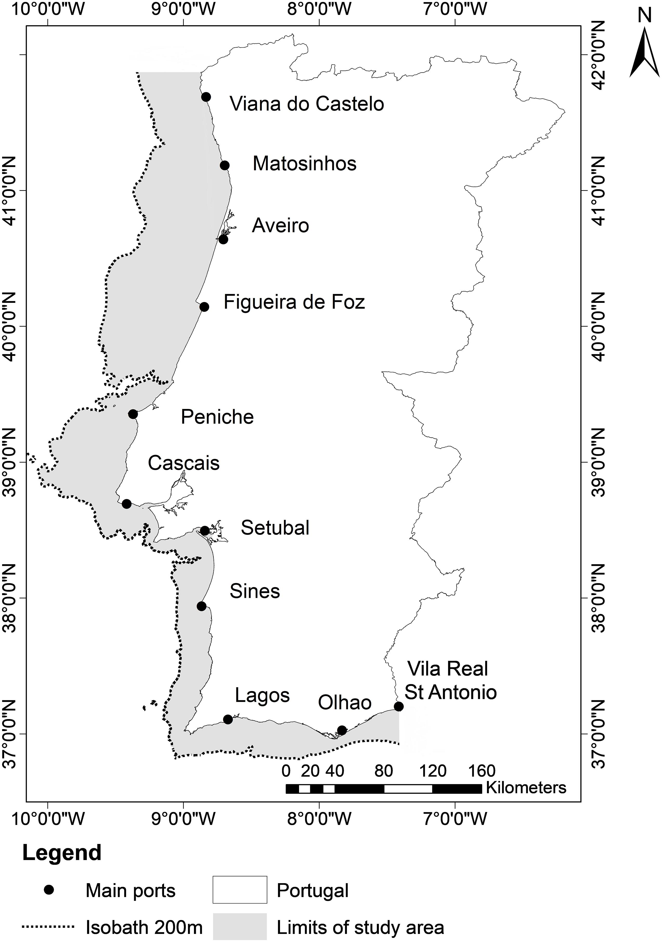
Figure 1. Map showing limits of the study area (200 m isobath).

Data and Model

In order to test the hypothesis of the occurrence of regime shifts in the PCSE during the last 30 years, we used data describing ecosystem drivers that include: (1) fishing mortality, (2) environmental variables and climatic indices, and data describing ecosystem state that includes: (1) observed biomass, (2) modelled biomass, and (3) ecosystem indicators (Table 1 and Figure 2).

TABLE 1

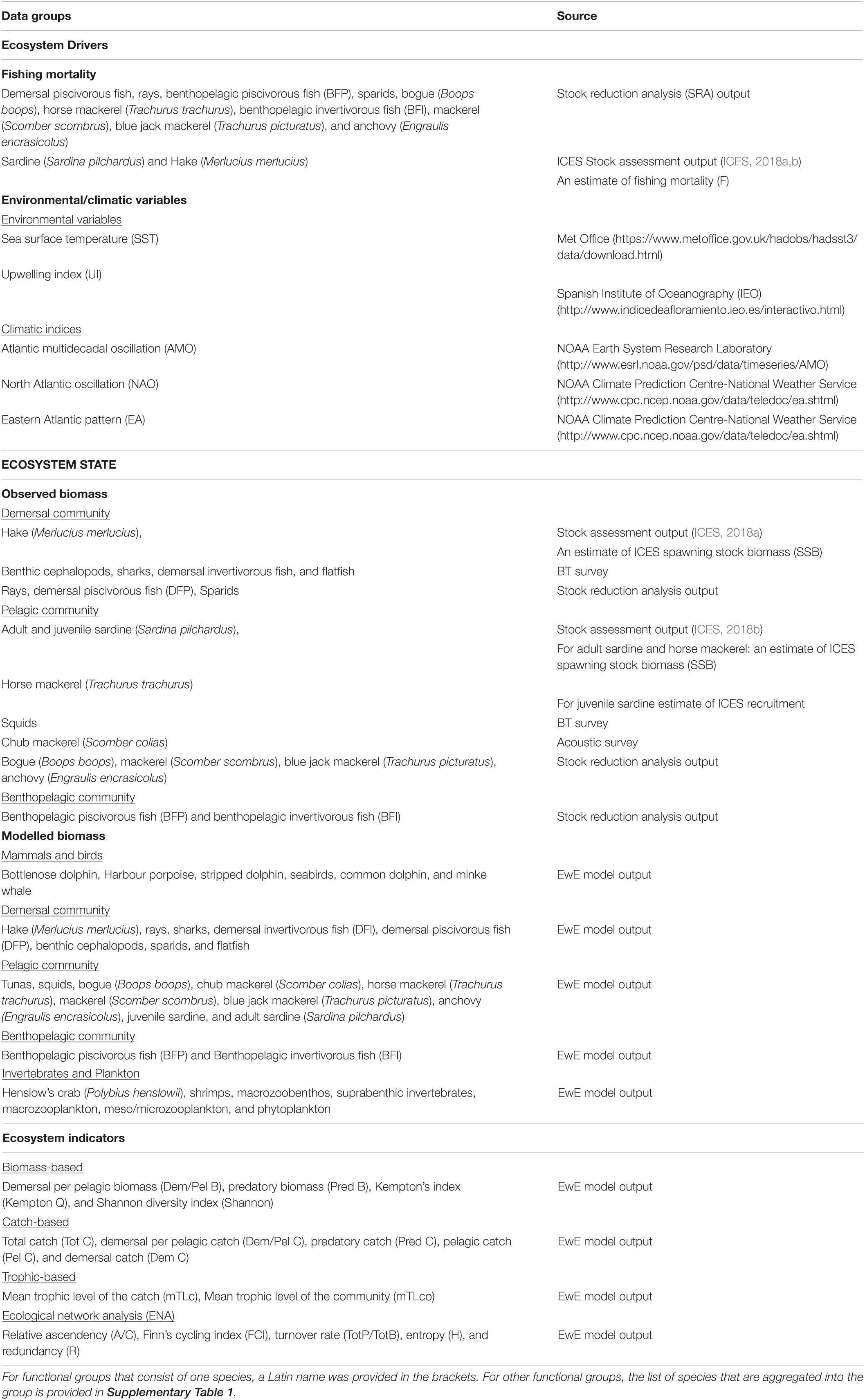
Table 1. Groups of data used in integrated trend analysis (ITA) and their sources.

FIGURE 2

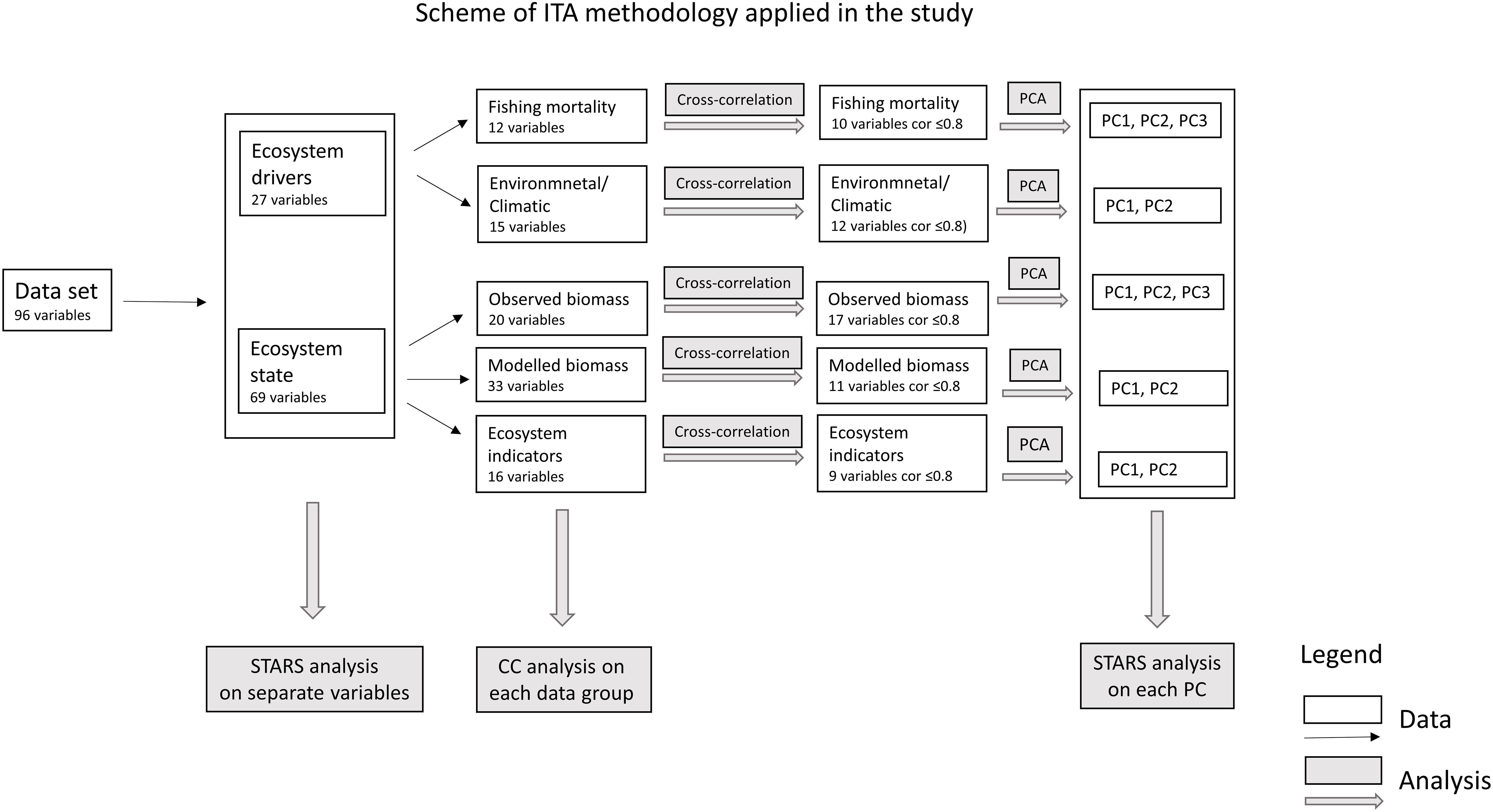
Figure 2. Scheme of integrated trend analysis (ITA) methodology applied in this study.

Fishing mortality and observed biomass data used in this study were also used as inputs of the EwE model, describing the PCSE between 1986 and 2017. The static version of this model was developed by Veiga-Malta et al. (2019) and further updated and fitted to 32 years of time-series data by Szalaj et al. (2021). Moreover, modelled biomass and ecosystem indicators data used in the study come as an output of this EwE model. The model was developed using the EwE modelling software that uses a set of differential equations to describe the ecosystem’s food web structure, its functioning, and dynamics. It has been described in detail by Christensen and Pauly (1992); Pauly et al. (2000), and Christensen and Walters (2004) (see text footnote 1). Using EwE data to assess the PCSE, allows for the integration of time-series data into the analysis that are not available from other sources, such as biomass of lower TL species and marine mammals. The EwE model estimated these groups and using them in the ITA provides a more complete picture of the studied ecosystem. In addition, the EwE model provided an extensive suite of indicators describing the ecosystem’s properties, its structure and functioning. The use of these data allows for the assessment of the changes that occurred in the PCSE at the whole ecosystem level. Model description and details regarding model parametrization are available in the study by Szalaj et al. (2021). In summary, the model covers the area of the Portuguese Continental Shelf (0–200 m; ICES subdivisions IXa), consists of 33 functional groups (Figure 3) and includes three fishing fleets: bottom trawl (BT), pelagic and multi-gear. Functional groups aggregate the species that live in a similar environment and have a similar diet. A detailed description of species that comprise each functional group is available in the Supplementary Table 1.

FIGURE 3

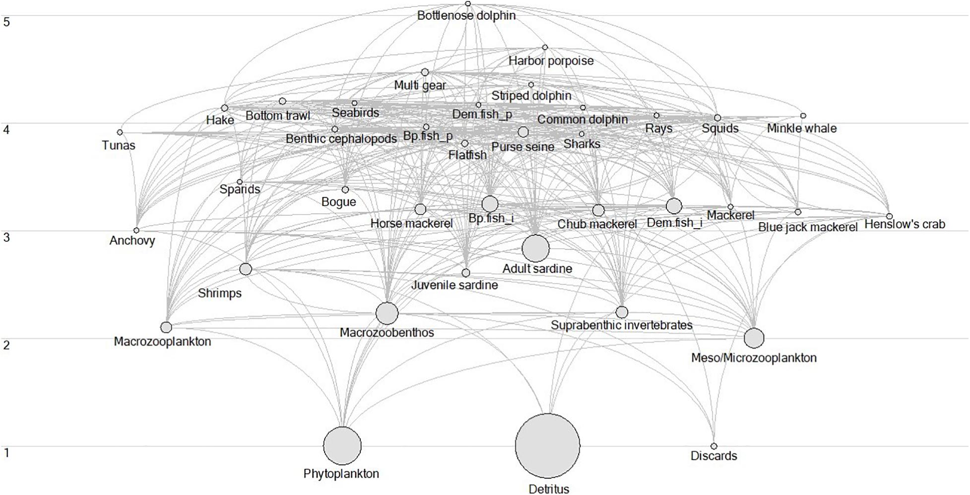
Figure 3. Flow diagram of the Portuguese continental shelf ecosystem (PCSE) in 1986. The list of species and functional groups are described in Veiga-Malta et al. (2019). Acronyms Bp.fish_p is Benthopelagic piscivorous fish, Bp.fish_i, is Benthopelagic invertivorous fish, Dem.fish_i, is Demersal invertivorous fish, Dem.fish_p, is Demersal piscivorous fish, and Suprabenthic inv is Suprabenthic invertebrates.

Ecosystem Drivers Data

Data describing ecosystem drivers consisted of two data groups: (1) fishing mortality and (2) environmental variables and climatic indices (Table 1). Fishing mortality (F) data for the majority of functional groups was calculated using Stock reduction analysis (SRA; Kimura et al., 1984) and implemented as a stochastic SRA (Walters et al., 2006) while F for sardine and hake was obtained from stock assessment outputs (ICES, 2018a, b). A detailed description of the SRA methodology and obtained results are provided in the Supplementary Material S2. Environmental variables consisted of annual, summer and winter means of SSTs and UI while climatic indices included annual, summer and winter means of AMO, NAO, and East Atlantic pattern (EA).

Ecosystem State Data

Data describing ecosystem state consisted of three data groups: (1) observed biomass, (2) modelled biomass, and (3) ecosystem indicators.

Observed biomass data

Observed biomass data consisted of the biomass data aggregated into 20 functional groups (Table 1). These data were used to calibrate the PCSE EwE model between 1986 and 2017 (Szalaj et al., 2021). When possible we used the outputs of stock assessment models as biomass estimates (i.e., sardine, hake and horse mackerel). For other species, when enough data were available, we estimated plausible biomass (B_SRA) trends using SRA. For the majority species (demersal piscivorous fish, rays, sparids, bogue, benthopelagic invertivorous, and piscivorous fish, mackerel, blue jack mackerel) we used BT survey data as abundance estimates for SRA input, with the exception of anchovy for which we used abundance estimates obtained from acoustic surveys. For species that lacked sufficient data to perform a SRA, the abundance index trends were taken directly from BT surveys (sharks, squids, benthic cephalopods, flatfish, and demersal invertivorous fish), with exception of the biomass for chub mackerel which was taken from an acoustic survey. Portuguese BT surveys are carried out in autumn (September–October) at predefined stations in the Portuguese Exclusive Economic Zone at depths varying from 20- to 500-m depth (ICES, 2017b). In this study only data that referred to the continental shelf (depth < 200 m) was considered. BT survey biomass estimates were calculated using the swept area method. Portuguese acoustic surveys (PELAGO survey series) are performed annually in spring (April–May) in an area that covers the Portuguese continental shelf. Acoustic fish data were obtained following the methodology described in ICES (2016) by performing echo-integration along 1 nm Elemental sampling distance unit (ESDU, distance measure used in acoustic surveys) and supported by fish sample collection. Both acoustic and BT surveys were performed by the Portuguese Institute of Sea and Atmosphere (IPMA).

Modelled biomass data

Modelled biomass data for 33 functional groups that range from plankton to marine mammals (Figure 3 and Table 1) were obtained from the EwE model fitted to the time series for the PCSE between 1986 and 2017 (Szalaj et al., 2021). A full list of functional groups used in this study is presented in Supplementary Table 1.

Ecosystem indicators data

Various indicators that describe ecosystem properties were extracted from the EwE model fitted to the time series for the PCSE between 1986 and 2017. Among the available indices, 16 indicators that represent distinctive processes, were used in the analysis. They are (1) demersal per pelagic biomass (Dem/Pel B), (2) predatory biomass (Pred B), (3) Kempton’s index (Kempton Q), (4) Shannon diversity index (Shannon), (5) total catch (Tot C), (6) demersal per pelagic catch (Dem/Pel C), (7) predatory catch (Pred C), (8) pelagic catch (Pel C), (9) demersal catch (Dem C), (10) mean trophic level of the catch (mTLc), (11) mean trophic level of the community (mTLco), (12) relative ascendency (A/C), (13) Finn’s cycling index (FCI), (14) turnover rate (TotP/TotB), (15) entropy (H), and (16) redundancy (R). Their definitions are presented in Table 2.

TABLE 2

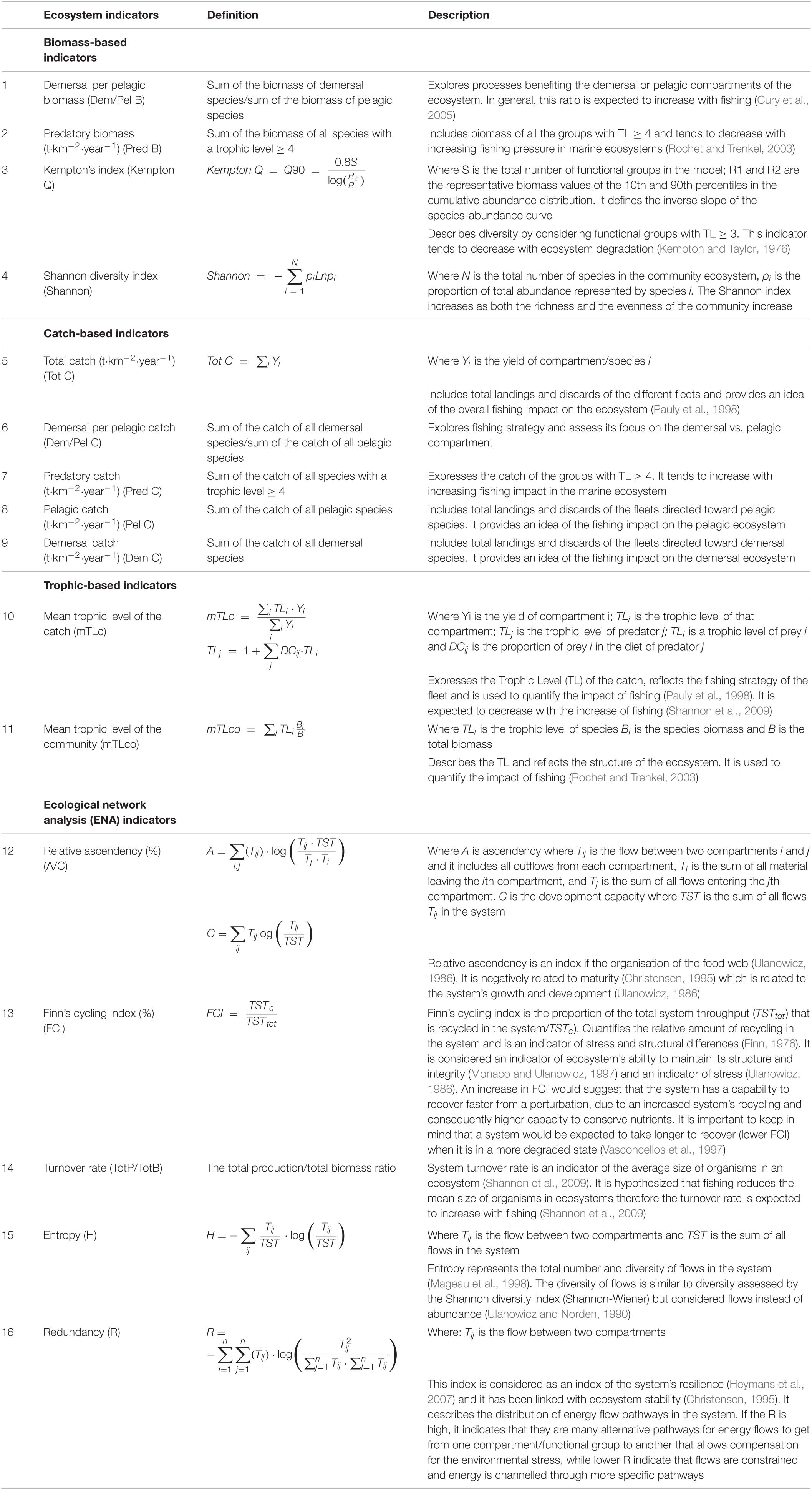
Table 2. Ecosystem indicators calculated from Ecopath with Ecosim (EwE), that describe the Portuguese continental shelf ecosystem (PCSE) between 1986 and 2017.

Integrated Analysis

Data described in subsection “Data and Model” was subjected to an ITA that was performed using the method described by Diekmann and Möllmann (2010) (Figure 2). It integrates the following statistical methods: (1) PCA, (2) STARSs (Rodionov, 2004), and (3) CC (Legendre et al., 1985). The PCA and CC analyses were performed using R (R Core Team, 2020), packages vegan (Oksanen et al., 2019) and rioja (Juggins, 2020). The script was obtained from Diekmann et al. (2012). The STARS analysis was performed using STARS software written in visual basic for application (VBA) Excel 2002, available at: sites.google.com/climateologic/download.

The PCA, based on the correlation matrix, was performed separately on fishing mortality data (PCA_FM), environmental/climatic variables (PCA_ENV_CLIM), observed biomass (PCA_B_obs), modelled biomass (PCA_B_model) and ecosystem indicators (PCA_indices). Before analysis, each dataset was checked for cross-correlation (Pearson) and variables that are highly correlated (>0.8, Supplementary Material S3) were excluded from the PCA. The list of the variables included in the PCA analysis is shown in Table 3. The number of meaningful principal components (PC) that were considered further in the analysis was assessed by the scree plot that shows how much variation each PC captures from the data and the broken stick plot that demonstrates how many PCs should be retained. Also, variable loadings for each meaningful PC were checked and the variables whose loadings values were < 0.3 were excluded from further analysis. Year scores for the meaningful principal components (mainly PC1 and PC2) were plotted against time to display temporal relationships (PC trends). Then PC trends were subjected to STARS analysis to detect the occurrence of regime shifts in the ecosystem. Moreover, the relationship between PC trends extracted from the data describing ecosystem state and ecosystem drivers were explored with cross-correlation. To identify significant shifts in mean values of a given time series, STARS was performed separately on each time series of the whole dataset and on the time series of PC scores (PC trends). The STARS method is based on a sequential analysis of change points in the time series using the Student t-test. At each observation, the procedure calculates a regime shift index (RSI) to determine whether the following observation values are significantly different from the mean of the previous regime. The method and its use in the detection of shifts in marine systems were discussed in Strinimann et al. (2019). In order to account for serial correlations (red noise component), the prewhitening procedure that adjusts the significance level of the shifts by calculating effective degrees of freedom, described in Rodionov (2006), was used. In this study the red noise component was modelled by the first-order autoregressive model (AR1) and estimated based on the ordinary least squares (OLS) as suggested by Marriot and Pope (1954) and Kendall (1954). Parameters that control the scale and magnitude of potential regime shifts (significance level and cut-off length) and weights assigned to outliers (Huber’s weight parameter) were set a priori to 0.05, 10, and 3, respectively according to Tomczak et al. (2013) and Heymans and Tomczak (2016). The magnitude of the detected regime shifts was assessed using RSI when the positive value indicates an increase and the negative value indicates a decrease.

TABLE 3

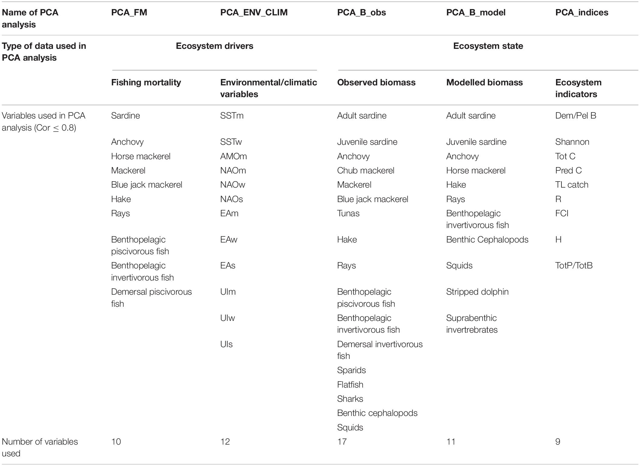
Table 3. Variables used in principal component analysis (PCA) after selection process (criteria for selection: cross-correlation ≤ 0.8).

The CC discontinuity analysis is a clustering technique that groups only sequential samples and has been used to identify the abrupt changes in time-series. It is used for multivariate datasets and clustering is based on the calculation of a similarity matrix of the time-series based on Euclidian distances. The CC analysis was performed separately on the same data groups as the PCA (fishing mortality, environmental/climatic variables, observed biomass, modelled biomass, and ecosystem indicators). According to Diekmann and Möllmann (2010), the significance level α (considered as a clustering-intensity parameter) and connectedness level were set to 0.01 and 50%, respectively. To make results interpretable in relation to PCA, data were standardised prior to the calculation of the similarity matrix.

Results

Ecosystem Changes, Key Functional Groups, and Key Drivers (PCA)

In PCA_FM that included fishing mortality variables, three PCs that in total explained 72.8% of variance were retained (Table 4). The time trajectory of PC1_FM presented a relatively stable trend until around 1998, followed by a decrease till the end of the study period (Figure 4A). Variables that contributed the most and positively related to this PC trend were fishing mortality of demersal piscivorous fish and rays (Table 4). The trend of PC2_FM showed an initial decrease until 1996, followed by an increase till 2006 and a further slight decrease until the end of the study period (Figure 4A). The variables that positively contributed to this trend were fishing mortality of benthopelagic invertivorous fish and mackerel, while fishing mortality of benthopelagic piscivorous fish, anchovy and hake contributed negatively (Table 4).

TABLE 4

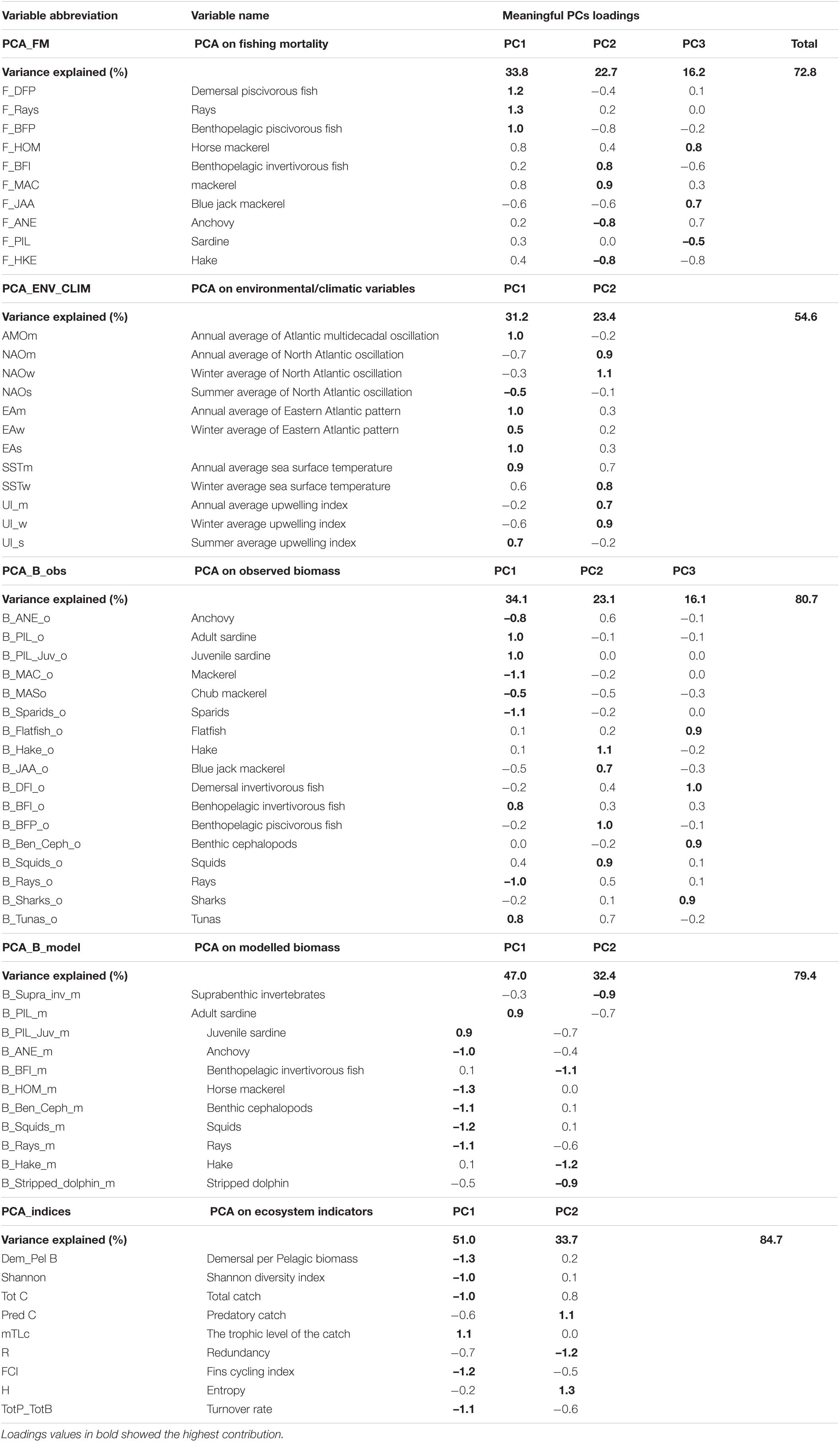
Table 4. Contribution of each variable to meaningful principal components for each PCA performed.

FIGURE 4

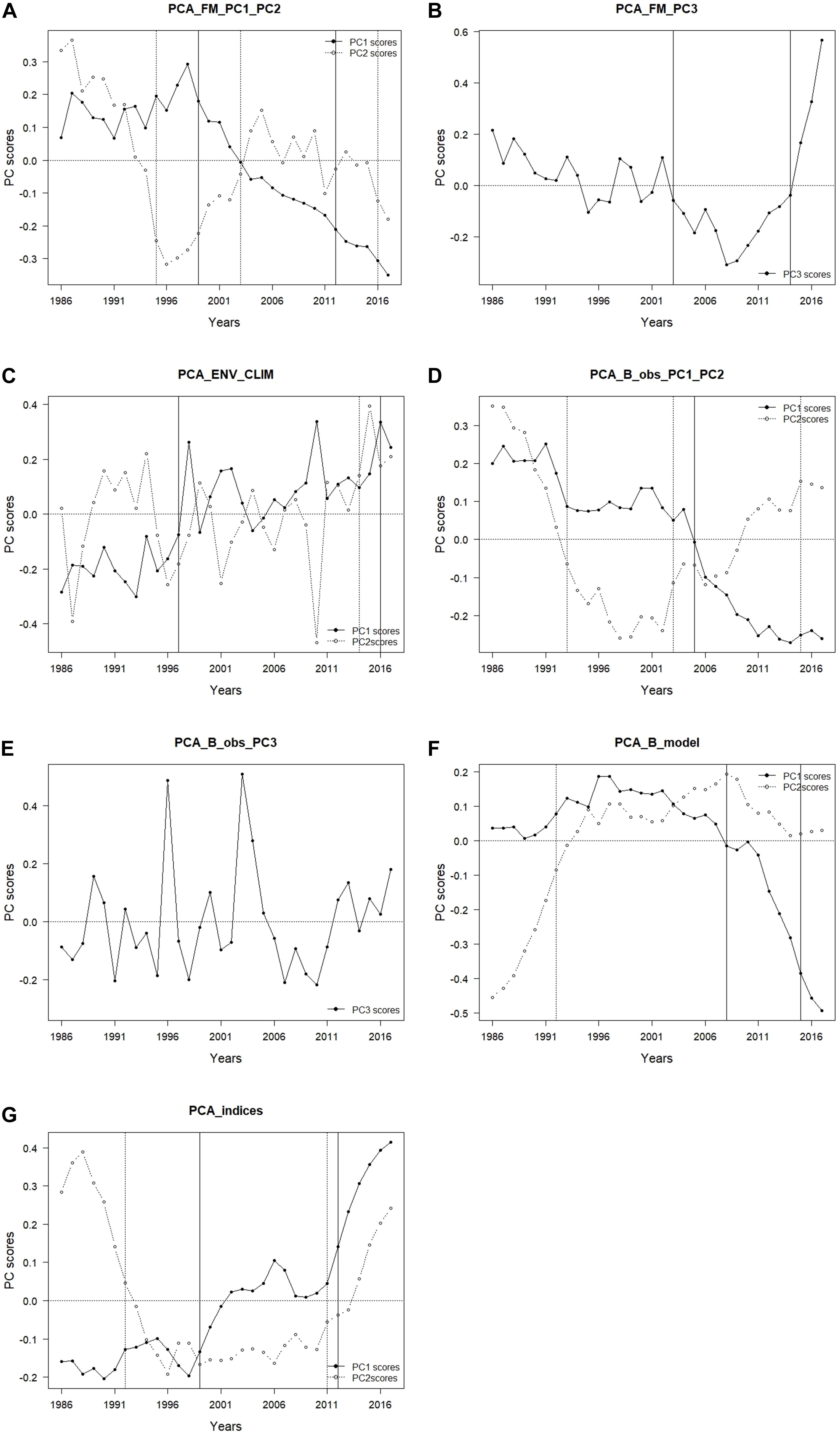
Figure 4. Results of principal component analysis (PCA); time-trajectory of PC scores of PCA performed on (A) fishing mortality PC1 and PC2 (PCA_ FM_PC1_PC2); (B) fishing mortality PC3 (PCA_FM_PC3); (C) environmental/climatic variables PC1 and PC2 (PCA_ENV_CLIM); (D) observed biomass PC1 and PC2 (PCA_B_obs_PC1_PC2); (E) observed biomass PC3 (PCA_B_obs_PC3); (F) modelled biomass PC1 and PC2 (PCA_B_model); and (G) ecosystem indicators PC1 and PC2 (PCA_indices) (black dots – PC1, PC3 white dots – PC2).

The trend of PC3_FM showed an initial gradual decrease with time till about 2008, followed by a sharp increase till the end of the study period (Figure 4B). The variables that contributed positively to this PC trend were fishing mortality of blue jack mackerel, horse mackerel (both positively) and sardine (negatively) (Table 4).

In the PCA_ENV_CLIM that included environmental/climatic variables, two retained PCs explained in total 54.6% of the variance (Table 4). The trend of PC1_ENV_CLIM showed a gradual increase with time and variables SST, AMO and EA showed the largest positive contribution to this trend (Table 4 and Figure 4C). The time trajectory of PC2_ENV_CLIM fluctuated till 2010 without any clear trend, then increased substantially (Figure 4C). This trend was mainly explained by NAO and UI (both annual and winter averages) (Table 4).

In the PCA_B_obs that included EwE input biomass data, three retained PCs explained 73.5% of the variance (Table 4). The time trajectory of PC1_B_obs which explained 33.8% of the variance, showed a decreasing trend that represented the biomass trend of sardine and benthopelagic invertivorous fish (Table 4 and Figure 4D). The variables that showed an opposite trend to PC1_B_obs were pelagic fish (anchovy and mackerels), sparids and rays (Table 4). Time trajectory of PC2_B_obs that explained 23.7 % of the variance and showed an initial sharp decrease until 1998 followed by a decrease (Figure 4D) represented the biomass trend for blue jack mackerel, hake, demersal piscivorous fish and squids (Table 4). The trend of PC3_B_obs that explained 15.9 % of the variance, did not show any clear tendency and reflected the biomass of demersal invertivorous fish and benthic cephalopods (Table 4 and Figure 4E).

In the PCA_B_model that included EwE output biomass data, two retained PCs explained 79.4% of the variance. The time trajectory of PC1_B_model fluctuated without any clear trend till around 2006, when it substantially decreased (Figure 4F). It represented the modelled biomass trend for sardine (Table 4). The opposite trend was observed for other pelagics (horse mackerel and anchovy), cephalopods and rays. The trend of PC2_B_model increased till 1996, then stabilised and fluctuated till the end of the study period (Figure 4F). It reflected the opposite trend to modelled biomass of hake, benthopelagic invertivorous fish, suprabenthic invertebrates and striped dolphin (Table 4).

Both PC1_indices and PC2_indices explained 51.0 and 33.7% of the total variance, respectively (Table 4). The time trajectory of PC1_indices showed an increasing trend (Figure 4G) that reflected the trend of mTLc (Table 4). The opposite trend to PC1_indices was observed for Tot C, Dem/Pel B, diversity (Shannon), and ENA indices (FCI, and TotP/TotB) (Table 4). The trend of PC2_indices sharply decreased until 1996, stabilised and since 2010 increased again (Figure 4G). The variables that reflected this trend were Pred C and H while R showed the opposite trend (Table 4).

Relationship Between Ecosystem Drivers and Ecosystem State

The PC trends extracted from the observed biomass data group showed significant correlations with PC trends extracted from fishing mortality and environmental/climatic data groups (Table 5). The statistical correlation was observed between PC1_B_obs and PC1_FM (R = 0.82, p < 0.01), PC1_ENV_CLIM (R = −0.66, p < 0.01) and PC3_FM (R = 0.35, p = 0.05). The largest correlations for PC2_B_obs and PC3_B_obs were found for PC2_FM (R = 0.68, p < 0.01) and PC2_ENV_CLIM (R = 0.38, p = 0.03), respectively.

TABLE 5

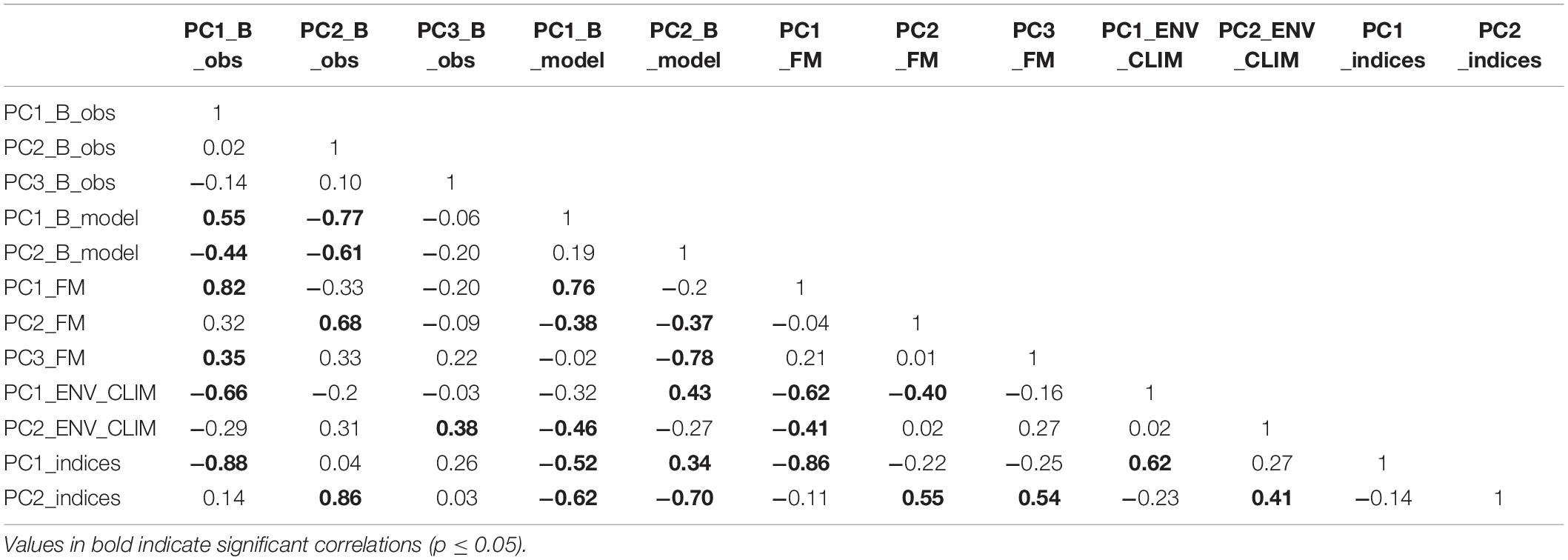
Table 5. Spearman cross-correlation between PCs extracted from different groups of data.

A statistical correlation was also found between PC trends extracted from modelled biomass and ecosystem drivers’ data (Table 5). Here, the PC1_B_model had the largest statistically significant correlation with PC1_FM (R = 0.76, p < 0.01) followed by PC2_ENV_CLIM (R = −0.46; p < 0.01) and PC2_FM (R = −0.38, p = 0.03). On the other hand, PC2_B_model shown the largest correlation with PC3_FM (R = −0.78, p < 0.01), followed by PC1_ENV_CLIM (R = 0.43, p = 0.01) and PC2_FM (R = −0.37, p = 0.04).

Also, statistical correlations were found between the PC trends extracted from the ecosystem indicators data group and both types of ecosystem drivers (Table 5). PC1_indices had the largest correlation with PC1_FM (R = −0.86, p < 0.01) followed by PC1_ENV_CLIM (R = 0.62, p < 0.01) while PC2_indices showed the largest correlation with PC2_FM (R = 0.55, p < 0.01), PC3_FM(R = 0.54, p < 0.01) followed by PC2_ENV_CLIM (R = 0.41, p = 0.02).

Regime Shift Detection (STARS and CC)

Significant shifts detected by STARS were observed for many variables representing ecosystem drivers and ecosystem state (Figures 5–8 and Supplementary Table 4).

FIGURE 5

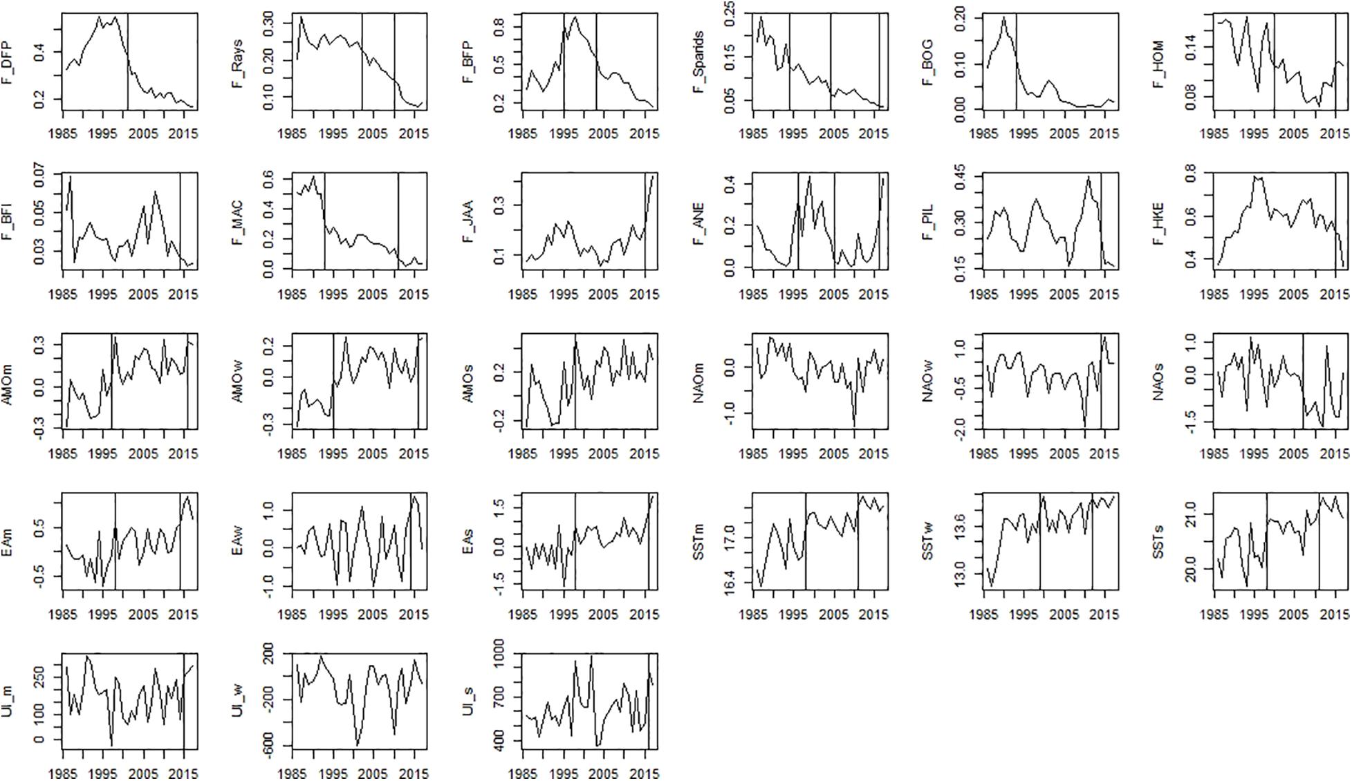
Figure 5. Time-series of ecosystem drivers data that includes fishing mortality and environmental/climatic variables. Significant shifts detected by STARS analysis are displayed on the plots as solid and dashed vertical line for shifts significant at p ≤ 0.05 and ≤0.1, respectively. Abbreviations, used in the figure, are explained in Supplementary Table 4.

FIGURE 6

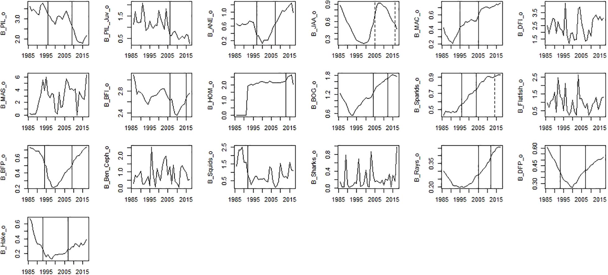
Figure 6. Time-series observed biomass data. Significant shifts detected by STARS analysis are displayed on the plots as solid and dashed vertical line for shifts significant at p ≤ 0.05 and ≤0.1, respectively. Abbreviations, used in the figure, are explained in Supplementary Table 4.

FIGURE 7

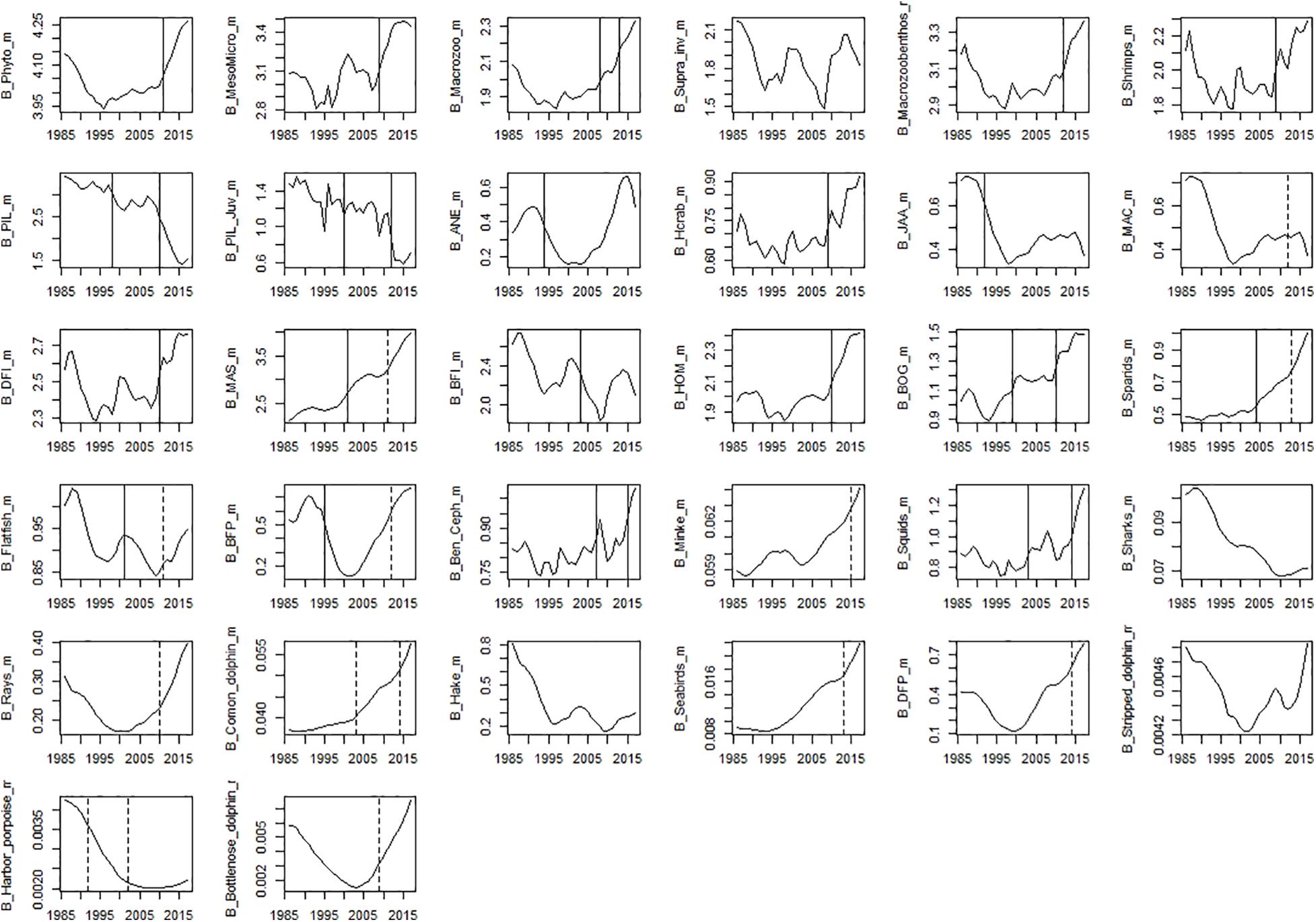
Figure 7. Time-series of modelled biomass data. Significant shifts detected by STARS analysis are displayed on the plots as solid and dashed vertical line for shifts significant at p ≤ 0.05 and ≤0.1, respectively. Abbreviations, used in the figure, are explained in Supplementary Table 4.

FIGURE 8

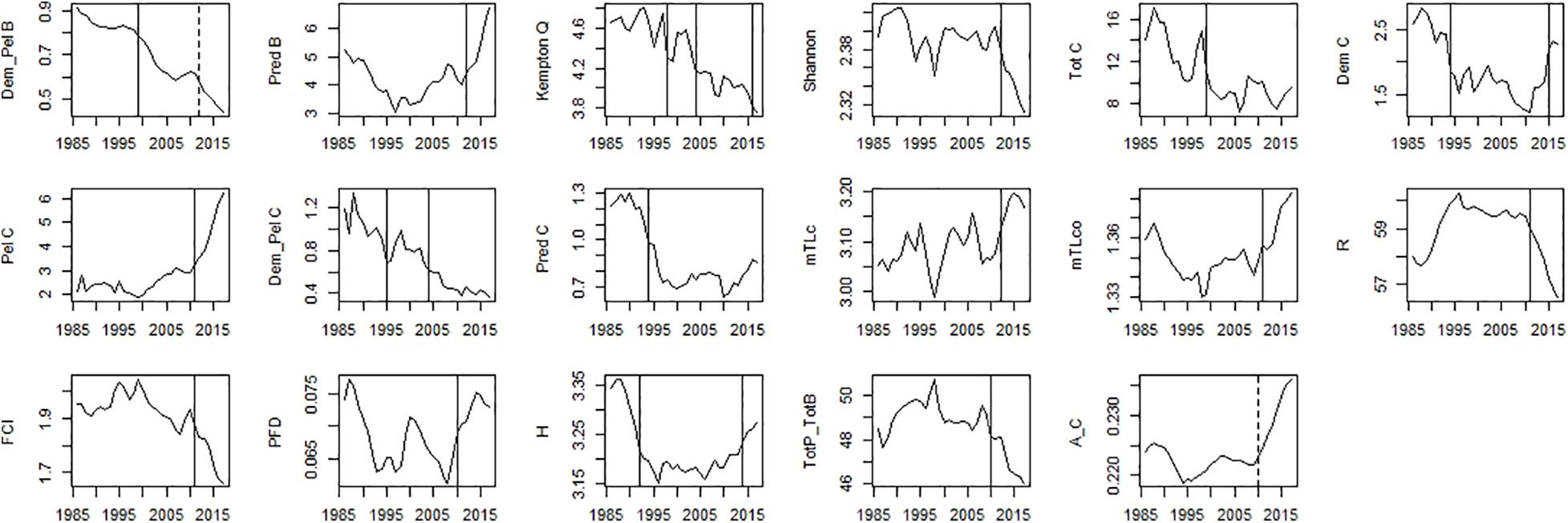
Figure 8. Time-series of ecosystem indicators data. Significant shifts detected by STARS analysis are displayed on the plots as solid and dashed vertical line for shifts significant at p ≤ 0.05 and ≤0.1, respectively. Abbreviations, used in the figure, are explained in Supplementary Table 4.

Among fishing mortality variables, significant shifts in the mid-90s were observed for fishing mortality of sparids, bogue, mackerel, benthopelagic piscivorous fish, and anchovy (Figure 5). The second shift in the mid-2000s was observed for fishing mortality of piscivorous fish, rays, sparids, and among small pelagic fish (SPF) for horse mackerel and anchovy (Figure 5). The last shift in the mid-2010s was observed for fishing mortality of all species (excluding fishing mortality of piscivorous fish and bogue).

Considering environmental/climatic variables, STARS detected significant shifts in the SST, AMO, EA in the mid-90s, followed by mid-2010s (2011–2016) (Figure 5). For NAO and UI, STARS detected only one shift in the mid-2010s (2014–2016) (Figure 5).

Among observed biomass variables, STARS detected significant shifts in the mid-90s for sardine, anchovy, mackerel, sparids, piscivorous fish, squids and hake. The second shift in the mid-2000s was observed for benthopelagic invertivorous fish, bogue, sparids, and rays. The last shift in the mid-2010s was observed for benthopelagic invertivorous fish and SPF (horse mackerel and bogue) (Figure 6). For modelled biomass variables, STARS detected significant shifts mainly in the mid-2000s and mid-2010s. In the mid-90s a shift in biomass was detected only for sardine, anchovy, blue jack mackerel, bogue, and benthopelagic piscivorous fish. In the mid-2000s the shifts were detected in the biomass of cephalopods, lower TL groups and invertebrates, chub mackerel and fish feeding on invertebrates. Further shifts in the mid-2010s, were detected for sardine and other SPF (horse mackerel, chub mackerel, and bogue), cephalopods and lower TL functional groups (Figure 7).

For ecosystem indices, significant shifts were mainly detected in the mid-90s and mid-2010s. The shift in the mid-2000s was only detected for Dem/Pel C and Kempton Q (Figure 8). Shifts in the mid-90s were detected for catch related indices (Tot C, Dem C, Pred C, and Dem/Pel C), Dem/Pel B, Kempton Q and H (Figure 8). Shifts after 2010 were detected for Pred B, diversity indices (Kempton Q, Shannon), catch related indices (Dem C, Pel C, and mTLc) and ENA indices (FCI, R, H, and Tot P/Tot B) (Figure 8).

Shifts at similar times were also detected by STARS performed on PCA results (PC trends) and CC analysis performed on separate data groups (Table 6). When performed on PC trends extracted from the fishing mortality data, STARS indicated that significant shifts occurred mainly in 1995 and 1999 (for PC2_FM and PC1_FM, respectively), 2003 (for PC2_FM), and 2012–2016 (for PC1_FM and PC2_FM), while CC detected discontinuity in the fishing mortality data in 1992 and 2003 (Table 5).

TABLE 6

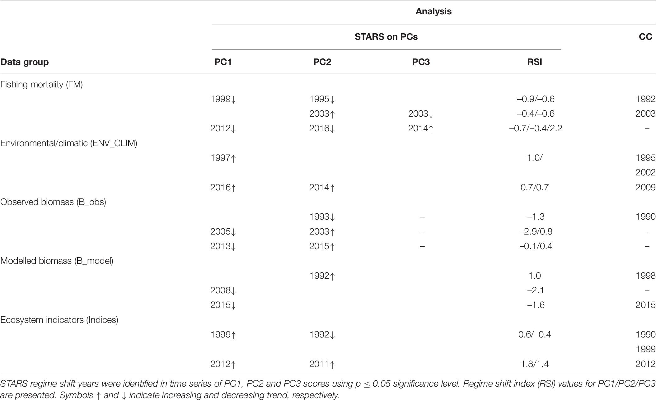
Table 6. Results of the sequential t-test analysis of regime shift (STARS) on principal component analysis (PCA) output and chronological clustering (CC) analysis.

For STARS performed on PC trends of environmental/climatic variables significant shifts were detected in 1997 for PC1_ENV_CLIM and 2014–2016 for PC2_ENV_CLIM and PC1_ENV_CLIM, respectively while CC detected discontinuity in 1995, 2002, and 2009 (Table 6).

Considering PC trends of observed biomass, STARS detected significant shifts in 1993 for PC2_B_obs, 2003–2005 for PC2_B_obs and PC1_B_obs, respectively and 2013–2015 for PC1_B_obs and PC2_B_obs (Table 6). The CC detected significant discontinuity only in 1990 (Table 6).

When performed on PC trends extracted from modelled biomass data group, STARS detected significant shifts in 1992 (for PC2_B_model), 2008 (for PC1_B_model), and 2015 (for PC1_B_model) while, CC showed discontinuity in the modelled biomass data in 1998 and 2013 (Table 6).

For STARS performed on PC trends of ecosystem indicators, significant shifts in the ecosystem were detected in 1992 for PC2_indices, 1999 for PC1_indices, and 2011 and 2012 for PC2_indices and PC1_indices, respectively (Table 6). The CC showed discontinuity in the ecosystem indicators data in 1990, 1999, and 2012 (Table 6).

Discussion

This study provides a comprehensive overview of the changes observed in the PCSE in the last three decades (Figure 9). Ecosystem changes were assessed by using a large dataset that included information on ecosystem drivers and ecosystem state. Observed changes were confirmed by the detection of significant shifts in all used datasets.

FIGURE 9

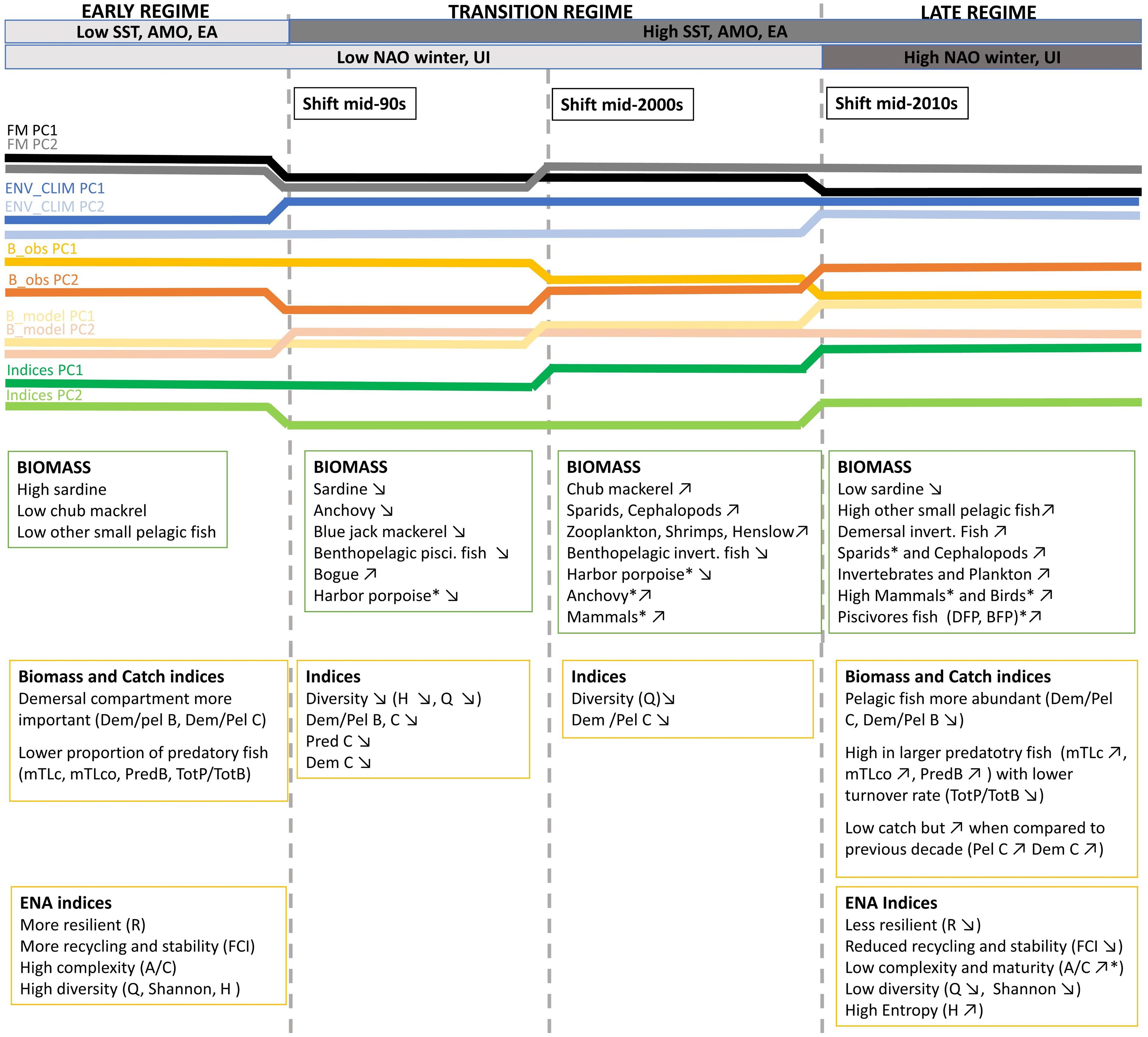
Figure 9. A conceptual diagram displaying the changes in the Portuguese continental shelf ecosystem (PCSE) between 1986 and 2017. Variable names marked by * means that for time series representing this variable shift was detected at p ≤ 0.1 significance level. For the remaining variables, shifts were detected at p ≤ 0.05. Detailed information about detected shifts that were summarised in the conceptual diagram is presented in Figure 5 and Supplementary Table 4. Abbreviations, used in the figure, are explained in Supplementary Table 4.

Description of PCSE Changes

Changes in Ecosystem Drivers

The major changes in the ecosystem drivers occurred in the mid-1990s. Firstly, we observed a decrease in the fishing mortality of most functional groups. This can be related to the substantial reduction of the Portuguese fleet that decreased by 30% between 1989 and 1996 (Instituto Nacional de Estatística, 1986-1996). Secondly, in the mid-90s, an increase in SST, AMO, and EA, has been reported. Around 1995, AMO entered a warm phase and since then the yearly SST means in North Atlantic including, the Iberian upwelling region has been ≥0.5°C higher than in the previous 65 years (Alheit et al., 2014). Later in the mid-2010s, we detected the change in winter NAO (that enters its high phase) and in the intensity of the upwelling. Changes observed in both these variables are in line with the findings by Borges et al. (2003) that demonstrated that in the Iberian shelf, high NAO phase is associated with more favourable upwelling winter wind conditions.

Changes in Ecosystem State (Biomass)

During the studied period, we have seen considerable changes in the biomass of many functional groups. In the mid-90s the biomass of sardine, the main commercial pelagic fish started to decline while an abundance of other SPFs such as bogue and chub mackerel increased. Later, in the mid-2000s further changes in the biomass of functional groups in the ecosystem have been reported. During this time, we observed not only a further decrease of sardine and increase of other pelagics but also an increase of lower TL groups (zooplankton and invertebrates), sparids and cephalopods started to be apparent. After 2010, we still observed a decrease in sardine with a concurrent increase of other SPF and lower TL groups. Additionally, during this time an increase in predatory, high TL and demersal fish has been detected.

Changes in Ecosystem State (Indicators)

Changes in the ecosystem were also reflected in the ecosystem indicators. The major changes in ecosystem indicators data were observed in the mid-90s and later in the mid-2010s.

In the mid-90s a major change was described by a decrease in Dem/Pel B, and catch related indices (Tot C, Dem C, Dem/Pel C, and Pred C). A decrease in Dem/Pel B can be explained by an increase in biomass of pelagic species, discussed above. On the other hand, a decrease in catch related indices is probably related to the reduction of fishing effort observed in the PCSE during the last three decades (Bueno-Pardo et al., 2020). Later in the mid-2010s, a further reduction in Dem/Pel B was observed. At this time, an increase in TL indices indicating a rise of higher TL fish has also been documented (mTLc, mTLco, Pred B, and Tot P/Tot B). Moreover, around this time, the indices that describe ecosystem stability and resilience shifted (FCI and R).

Causes of Ecosystem Changes

The correlation analysis indicates that the changes in ecosystem trends (biomass and indicators) are statistically correlated with the changes in fishing and environmental/climatic variables.

Fishing

Fishing has been documented as a major driver of the marine ecosystems worldwide (e.g., Pauly et al., 1998; Coll et al., 2008; Llope et al., 2011). Moreover, it has been highlighted as an important driver of the PCSE (Szalaj et al., 2021).

The important role of fishing detected in this study can be explained by the considerable changes observed in the Portuguese fishing sector in the last 50 years. Since the late 1980s, reported landings dropped approximately 52%, from 197,000 to 94,700 t in 2014 (Bueno-Pardo et al., 2020). Moreover, after the implementation of the European Common Fisheries Policy (EU CFP) (since 1983), a steady decrease of fishing effort started to be notable with a decrease of 75 and 50% in the number of boats and fishers, respectively (Leitão et al., 2014b). A decrease in fishing effort, observed after enforcement of EU CFP measures, could affect an increase in biomass of some species observed in the study. For example, an increase in predatory higher TL fish, that manifested after 2010 can be linked with the reduction in fishing pressure. Observed in this analysis, a decrease in fishing mortality of most functional groups since the mid-90s (demersal and benthopelagic piscivorous fish, rays, sparids, bogue, horse mackerel, and mackerel), might have positively impacted the high TL predatory fish and demersal fish whose abundance increased and shifted after 2015 (with a time lag). A link between fishing and high TL predatory fish established in this study is based not only on the biomass data (observed increase in the biomass of demersal and benthopelagic piscivorous fish) but also based on ecosystem indicators. An increase in indices, mTLc and mTLco, that are linked with the decreasing fishing pressure (Pauly et al., 1998; Rochet and Trenkel, 2003), were observed in this study. This is in line with the study by Leitão (2015a) that assessed the profiles of Portuguese fisheries landings since 1950. In this study, Leitão (2015a) documented an increase in the mean TL of the catch, by approximately 0.2 units per decade.

However, in this study, we used fishing mortality data for only 10 functional groups, and this considerably limits the assessment of the impact of fishing on this system. Fishing mortality data for eight commercial groups, that were included in the biomass data (chub mackerel, sparids, flatfish, demersal and benthopelagic invertivorous fish, cephalopods, and sharks) were not considered as fishing drivers.

Environmental/Climatic Drivers

The PC trends extracted from environmental/climatic drivers data showed significant correlations with all PC trends extracted from ecosystem data.

The importance of environmental variability to drive marine ecosystems has been reported worldwide (e.g., Parsons and Lear, 2001; Lehodey et al., 2020). This has been particularly prominent in the large upwelling systems (e.g., Shannon et al., 1976). The PCSE is located at the northern limit of the Canary Current upwelling system and during spring and summer it is affected by the seasonal upwelling (Wooster et al., 1976; Fiúza et al., 1982). Moreover, changes in the PCSE have been linked to environmental variability (e.g., Szalaj et al., 2021).

A decrease in sardine biomass and an increase in other pelagic fish and rays were both represented by PC1 in both data sets (observed and modelled biomass data groups). Additionally, in the observed biomass dataset, PC1 was represented by sparids, benthopelagic invertivorous fish, and tunas (for which data was not introduced in PCA_B_model) while for modelled biomass data set, PC1 was also represented by cephalopods. PC1_B_obs and PC1_B_model showed a statistically significant correlation with PC1_ENV_CLIM and PC2_ENV_CLIM, respectively. PC1_ENV_CLIM represented SST, AMO and EA variables, while PC2_ENV_CLIM represented NAO and UI trends. Therefore, based on this analysis it seemed that all these environmental/climatic variables might have played a role in the overall biomass changes observed in the study.

It is possible that the changes in environmental drivers that were apparent in the mid-90s (SST, AMO, EA) affected the ecosystem and manifested with different time lag depends on the functional groups. In the PCSE, the productivity of species representing the functional groups for which significant shifts were observed in the mid-2000s, has been already documented as being influenced by environmental variability. Firstly, we have a large number of studies that link sardine recruitment and productivity with SST, chlorophyll concentration (Chla) (Santos et al., 2012; Leitão et al., 2014a; Garrido et al., 2017), NAO, wind conditions (Santos et al., 2012; Leitão et al., 2014a) and coastal upwelling (Santos et al., 2001; Santos et al., 2012; Malta et al., 2016).

Moreover, other pelagic species such as Atlantic horse mackerel (T. trachurus) and anchovy (Engraulis encrasicolus) catch rates were linked with upwelling, the magnitude of northern wind and SST (Santos et al., 2001; Ullah et al., 2012; Leitão, 2015b). Also, among cephalopods, cuttlefish (Sepia oficinalis) catch rates were associated with the SST, winter NAO and autumn wind magnitude (Ullah et al., 2012). Furthermore, by using a statistical multi-model approach, Baptista et al. (2015) found that environmental factors such as winter SST and NAO affected short term variation of catch rates of common two-banded seabream (Diplodus vulgaris) in the south and southwest of Portugal. Also, they found that these species catch rates were associated with autumn and a yearly wind magnitude component, that can be treated as a proxy for the upwelling condition. All these studies were performed using statistical models. It is therefore encouraging that results from the study using different methods such as the outputs of ecosystem model and discontinuity analyses, established similar associations.

After 2010, we still observed a decrease in sardine and a concurrent increase in other SPF and lower TL groups. Additionally, during this time an increase in predatory, higher TL and demersal fish was also detected. When analysing shifts in data describing drivers, we observe that around this time the shift in winter NAO (that enters its high phase) and in the intensity of upwelling was detected. In the Iberian shelf, a high NAO phase is associated with more favourable upwelling winter wind conditions (Borges et al., 2003) that may favour lower trophic groups (phytoplankton, zooplankton, benthos). This can quickly promote the abundance of lower TL groups that rely directly on plankton as a food source (Barth et al., 2007). An increase in lower TL groups was initiated earlier in the mid-2000s but the shift in NAO in the mid-2010s might have further enhanced the change that initiated earlier.

Internal Drivers (Trophic Interactions)

The effect of environmental variability on some species (functional groups) might have been intensified by the internal, trophic interactions that exist between these species. The importance of trophic interactions in the dynamics of the marine ecosystems has been well documented worldwide (e.g., Coll et al., 2008; Alexander et al., 2015). Also, it has been demonstrated as the main factor driving PCSE dynamics between 1986 and 2017 (Szalaj et al., 2021).

In the context of this study, an increase in lower TL groups due to the environmental conditions, could pronounce trough the food web and promote the abundance of fish of prey that consequently might have benefited the groups at higher TL including cephalopods, demersal fish, and higher TL predatory fish. Also, the effect of environmental variability on some species (functional groups) might be exaggerated by the existence of the predator-prey loop between these species. This can be a case for sardine and chub mackerel. The increase in the biomass of chub mackerel observed after 2001 (that possibly benefited from increased temperature) may have caused increased pressure on sardine recruitment as it has been established that sardine eggs are chub mackerel’s preferred prey (Garrido et al., 2015). At the same time, increased biomass of other species such as bogue, horse mackerel and mackerel might have added pressure on sardine due to the predation on its eggs and juveniles (Garrido et al., 2015).

Implications to Ecosystem Structure and Function (ENA Indices)

Other than the changes evident from the direct observations and modelled biomass, the ENA indices provide information about the changes that occurred at the whole ecosystem level. Analysis of ENA indices showed that not only has the abundance of functional groups altered but also the cycles and pathways that are implied by the ecosystem food web showed considerable alterations within the last thirty years.

ENA indices (R, FCI, and A/C), indicate that after 2010, the ecosystem became less stable and less resilient with reduced maturity and complexity. Lower stability and resilience, reflected by the R, is implied by the reduction in the number of pathways through which energy flow is transferred. Moreover, reduction in R and increase in A/C implies lower maturity of the system which become more constrained and less complex. Lower FCI indicates that the system’s recycling and its ability to conserve nutrients are reduced and therefore, its capacity to endure in the face of resource scarcity has diminished. These characteristics indicate structural differences (Finn, 1976) and decreased stability (DeAngelis et al., 1989; Loreau, 1994). Reduced resilience and stability concur with the observed decrease in diversity indices as it has been demonstrated that a system with greater biological diversity is usually more resilient than the one with less diversity (Oliver et al., 2015). It is not clear, what has caused the changes in the ecosystem structure and its flows. However, the most prominent change (the change of the highest magnitude) observed in the last decades was the decline of sardine. Indeed, the effects of the changes in dominant SPF on the ecosystem food web in the upwelling systems, have been broadly discussed (Cury et al., 2000). Moreover, based on the Ecopath model and description of the Iberian shelf food web structure, it has been demonstrated that sardine played an important role in the Iberian ecosystem, being an important key linkage between primary producers and top predators (Veiga-Malta et al., 2019). Moreover, the ecosim simulations demonstrated that sardine has an important role in a wasp-waist scenario (Szalaj et al., 2021). This confirmed its key role in the Iberian upwelling system as a biomass-dominant species at mid-TL s that channel most of the energy flow in the ecosystem. Therefore, it seems probable that sardine decline disturbed important trophic links and pathways through which the flow of energy passes. At the same time, the other SPF were not well linked to the rest of the food web with few animals predating on them and being not very important for the fishery. For example, bogue was only caught as a bycatch of the purse seine fishery and catches of chub mackerel only become important after 2000 when a decline of sardine occurred and fisheries managed to find alternatives for economic compensation (Instituto Nacional de Estatística, 2000-2018). Therefore, when pelagic energy flow was redirected to the other SPF (that were not as important prey for top predators and fisheries as sardine was before 1995), disruption in the energy flow pathways occurred. Consequently, ecosystem stability was reduced, and the ecosystem became less resilient. Similar changes were described in the Northern Benguela upwelling system, where a shift in dominant pelagic species coincided with the simplification of the food web and reduced resilience (Heymans and Tomczak, 2016).

Assessment of the Methodology

Methods that comprised of ITA methodology has been used to detect ecological and climatic regime shifts and they have been widely discussed and considered adequate (e.g., Rodionov and Overland, 2005; Möllmann et al., 2009; Diekmann and Möllmann, 2010; Tomczak et al., 2013). However, the use of EwE outputs in this type of analysis is rare and to our knowledge there are only two studies that applied this approach to detect and describe regime shifts. One in the Baltic Sea and the other in the Northern Benguela (Tomczak et al., 2013; Heymans and Tomczak, 2016). The main advantage of this approach is the possibility to use more data inputs, that EwE provides, for example, the data of functional groups for which observations do not exist and ecosystem indicators. Among the latter, ENA indicators can be especially valuable in the studies of ecosystem regime shifts as discussed by Tomczak et al. (2013). For example, the redundancy that was linked with ecosystem resilience (Heymans et al., 2007) is directly related to regime shift definition. Therefore, we argue that using this approach is very beneficial in the studies that aim to detect and describe ecosystem regime shifts.

However, we are aware of the limitations of our analyses, such as high cross and auto-correlations. Planque and Arneberg (2017) criticised the use of PCA as a method for ecosystem assessment of marine ecosystems because the ITAs inputs usually share a similar trend and have autocorrelation properties. The authors demonstrated that most of the patterns revealed by the PCA can emerge from random time-series and that the fraction of the variance that cannot be accounted by random processes is minimal. In the context of our study these findings are worrying and this limitation should be taken into consideration when interpreting the results. We tried to minimalize this effect by excluding highly correlated variables prior to PCA. Also, the ITA methodology used in this study combines different methods and not all of them rely on PCA. For example, STARS performed on separate time series accounts for autocorrelation (prewhitening method described in the “Material and Methods” section) and detected shifts in similar years (time ranges) that STARS performed on PCA output. Moreover, the CC method confirmed dissimilarity in the datasets in similar years as STARS on PCA results. However, to confirm and consolidate the conclusions of this study, as a future recommendation we would suggest to replicate the analysis using other methods that are not so sensitive to cross and autocorrelation and compare its outputs with the results obtained in this study.

Moreover, our analysis is fed with data that constitute the output of a modelling approach therefore our results are affected by the assumptions of the model. EwE is a commonly used approach (Colléter et al., 2015) and its best practices, pros and cons have been widely discussed (Heymans et al., 2016; Walters et al., 1997). When building and calibrating the EwE model for the PCSE, we considered the best practice guide (Heymans et al., 2016), reported uncertainties and thoroughly discussed limitations (Szalaj et al., 2021). Moreover, the model was well fitted to most groups with observation data, and we have confidence in the model and data it provided (Veiga-Malta et al., 2019; Szalaj et al., 2021). This was also reflected in this study because the results obtained from the analyses performed on observed biomass are in line with the results obtained from modelled biomass.

Regime Shifts in the PCSE and North Atlantic

The performed analyses allowed to detect three shifts in data, in the mid-90s, mid-2000s, and mid-2010s. However, based on the analysis of the results and the review of the literature, only two of them, in the mid-90s and mid-2010s, could be considered as shifts to a new regime.

The shifts in the mid-90s and mid-2010s were detected by STARS on all PC trends regardless of the data group used, while the shift in the mid-2000s was mainly detected in the biomass data (when considering main PCs). Moreover, the timing of the shifts detected in the mid-90s and mid-2010s in this study coincided with the time of ecosystem regime shifts documented in the other regions of the North Atlantic. The mid-90s shift is well documented in the northern hemisphere and a large set of previous studies described it and linked it with large scale atmospheric variations (e.g., Cabrero et al., 2018; Alheit et al., 2014; Beaugrand et al., 2015). For example, Alheit et al. (2014), linked the complex ocean-atmosphere changes in the mid-90s with a regime shift in the ecosystems of the Northeastern and Central Atlantic. He discussed that when in the mid-1990s, three events including (1) decrease of the NAO index, (2) the weakening of the Atlantic Meridional Overturning Circulation (AMOC), and (3) the contraction of the subpolar gyre (SPG) occurred, a substantial redistribution of water masses in the Northeast Atlantic happened. This affected most ecosystems in the region causing a change in the abundance of the small pelagic clupeoid fish and their northward migration. Moreover, Cabrero et al. (2018) demonstrated that in the Iberian shelf, sardine entered a new regime in the late 1990s triggered by large-scale ocean climate processes. He concluded that the combination of climate and oceanographic conditions, including NAO, EA, SST, AMO, and UI intensity, contributed to this regime shift.

Also, a reference to the mid-2010s shift in the Northern Atlantic appeared in the recent literature. For example, Tanner et al. (2020) found that the abrupt changes in the growth of two deep-sea scorpaenid fishes off the central islands of the Azores and the island of Madeira occurred not only in the late 90s but also around 2014. This coincides with a significant shift in the mid-2010s detected in this study. Tanner et al. (2020) associated the shift in 2014 with a large-scale abrupt biological shift that was predicted by Beaugrand et al. (2019) to occur after 2014 in response to a strong El Nino event that affected the Northern Hemisphere climate. In the study by Beaugrand et al. (2019), a model based on the numerically generated thermal niche of pseudo-communities was used and the shifts predicted by the model were validated with observed community shifts in 14 oceanic regions. This study is of special interest to us, as the shift in the mid-2010s, that was detected in our analysis, is not well documented in the scientific literature. A few substantial climate events occurred around this time: exceptionally cold North Atlantic Ocean temperatures, 2015 severe European heatwave (Duchez et al., 2016) and the change in AMO phase (Frajka-Williams et al., 2017). However, these events are quite recent, and their ecological consequences are not yet well studied and understood.

The mid-2000 regime shift that was detected in this study did not relate to any relevant environmental pressure observed in the North Atlantic in our dataset or the literature. Generally, the time between 2005 and 2014 is considered a relatively quiet period when referring to the climatic divers in the Northern hemisphere (Beaugrand et al., 2015). Moreover, this shift was not reflected in the changes observed in the ecosystem indicators analysed in the study. Therefore, we considered the period between the first shift in the mid-90s and the shift in the mid-2010s as the “transition regime” during which the changes triggered by a previous shift in the mid-90s manifested in the ecosystem with the time lag whose length depends on the functional group.

From this analysis it is not clear whether the shift was caused solely by the environmental/climatic causes because both analysed ecosystem drivers’ trends (fishing and environmental/climatic) correlated with ecosystem state trends. However, based on the literature and a well-documented climatic shift in the North Atlantic we can infer that climatic variability played a major role. However, the effect of fishing pressure should not be completely disregarded as fishing is a well-documented driver of marine ecosystems worldwide (e.g., Coll et al., 2008; Alexander et al., 2015) and substantial changes in the fishing sector has been documented during the last three decades in the PCSE (Leitão et al., 2014b; Bueno-Pardo et al., 2020). Moreover, regime shifts are commonly triggered by a combination of fishing and environmental/climatic factors acting together (e.g., Daskalov et al., 2007; Möllmann et al., 2009). In the case of the PCSE, although we have documented a decrease in fishing effort (Bueno-Pardo et al., 2020), many Portuguese fish stocks are considered overfished (Leitão, 2015a). As we discussed in section “Fishing,” the impact of fishing on the ecosystem has not been fully captured in this study. Therefore, the hypothesis of the fishing cause of the PCSE regime shift should be explored in future studies.

At this stage, it is impossible to say if the current regime is stable or reversible as the PCSE as an upwelling system might have a wide range of natural variability (Black et al., 2014). If the observed ecosystem food web changes are linked with sardine decline as discussed above (in the previous subsection) then it is unknown what effect sardine recovery may have on the ecosystem. The latest ICES sardine stock assessment indicated that the 2019 sardine recruitment estimate constitutes the highest value since 2004 and is above the long-term geometric mean (ICES, 2020). That might suggest that the sardine productivity trend is shifting. However, at that stage it is unknown whether the increase in sardine recruitment will continue and sardine stock will recover to the level prior to the mid-1990s and what impact would that potential increase have on the food web.

Implications for Management

The potential occurrence of regime shifts might have considerable implications for the productivity of the commercial stocks and consequently to the fisheries. Therefore, the awareness of regime shift in the management of the ecosystems is of utmost importance and should be included in the management plan of marine systems (deYoung et al., 2008). This management should include not only timely detection and adaptation to a new regime but also prevention (deYoung et al., 2008; Crépin et al., 2012). The latter is crucial and should focus on building and maintaining the resilience of desired ecosystem states (Levin and Lubchenco, 2008). Nevertheless, sometimes, regime shifts cannot be prevented, and in these circumstances, timely detection is important in order to act quickly to alleviate the adverse effects and adapt to a new reality (Crépin et al., 2012).

After the detection of regime shifts, the adaptation in the form of adaptive management should take place. For example, a regime-specific harvest rate strategy could be implemented when an indication toward a shift to an alternate ecosystem state exists (Polovina, 2005; MacCall, 2002). This study demonstrated that one of the possible mechanism behind the described regime shift is environmentally related therefore in the context of PCSE management, efforts should be focused on establishing reference points at which the change in environmental pressure might result in an abrupt change in the ecosystem (Large et al., 2015).

Conclusion

The ITA presented in this study pointed to the occurrence of two regime shifts in the PCSE in the mid-90s and around the mid-2010s. Interpretation of results allowed for the identification of three periods: “early regime” till the mid-90s, “transition regime” till mid-2010s, and “late regime” since the mid-2010s in the last three decades. Differences between “early regime” and “late regime” are evident in all components of the ecosystem and at multiple TLs. They include changes in species abundance as well as community composition. Moreover, ENA indices indicate that the internal food web structure and organisation of the ecosystem have changed. Specifically, detected regime shifts are characterised by changes in the pelagic community: (1) it became more dominant when compared to the demersal community; (2) a shift from the main commercial stock of sardine to less commercially viable small pelagics had occurred. Moreover, an increase in higher TL predatory fish and demersal fish was observed.

Changes described in the ecosystem were probably caused by two types of external drivers. First, environmental forcing (related to an increase in SST, AMO, EA, NAO, and intensification of the upwelling conditions) possibly affected lower TL groups and SPF, and second, reduction in fishing pressure probably benefited high TL predatory and demersal fish. Moreover, the internal triggers, related to indirect trophic interactions also might play a role in the observed ecosystem change. An increased abundance of lower TL functional groups and fish of prey might benefit higher TL groups such as cephalopods, demersal and predatory fish. Furthermore, the competition and intraguild predation between sardine and other pelagic fish might have contributed to the changes in the pelagic community.

Data Availability Statement

The raw data supporting the conclusions of this article will be made available by the authors, without undue reservation.

Author Contributions

DS conceptualized the study, wrote the original draft, conducted the modelling, performed statistical analyses, and interpreted the results. AS, PR, and HC conceptualized the study, contributed to the interpretation of results, reviewed the manuscript, and assisted in funding acquisition. All authors contributed to the article and approved the submitted version.

Funding

This publication was financed by Portuguese national funds through FCT – Fundação IP under project reference UIDB/04292/2020, and by the European Union’s Horizon 2020 Research and Innovation Programme under grant agreement N810139: Project Portugal Twinning for Innovation and Excellence in Marine Science and Earth Observation – PORTWIMS. Work of DS was funded by FCT (Fundação para a Ciência e a Tecnologia) Ph.D. fellowship (ref PD/BD/114540/2016).

Conflict of Interest

The authors declare that the research was conducted in the absence of any commercial or financial relationships that could be construed as a potential conflict of interest.

Supplementary Material

The Supplementary Material for this article can be found online at: https://www.frontiersin.org/articles/10.3389/fmars.2021.629130/full#supplementary-material

Footnotes

^ www.ecopath.org

References

Alexander, K. A., Heymans, J. J., Magill, S., Tomczak, M. T., Holmes, S. J., and Wilding, T. A. (2015). Investigating the recent decline in gadoid stocks in the west of Scotland shelf ecosystem using a foodweb model. ICES J. Mar. Sci. 72, 436–449. doi: 10.1093/icesjms/fsu149