 Nathan D. McTigue
 Quentin A. Walker
 Carolyn A. Currin
- 1National Oceanic and Atmospheric Administration, National Centers for Coastal Ocean Science, Beaufort, NC, United States
- 2CSS-Inc., Fairfax, VA, United States
Coastal wetlands have sediments that contain organic matter preserved against decomposition for timespans that can range up to millennia. This “blue carbon” in wetland sediments has been proposed as a sink for atmospheric carbon dioxide and a potential source of greenhouse gases if coastal habitats are lost. A missing gap in the role of coastal habitats in the global carbon cycle is elucidating the fate of wetland sediment carbon following disturbance events, such as erosion, that can liberate organic matter to an oxygenated environment where decomposition can more readily occur. Here, we track the fate of previously stored salt marsh sediment by measuring the production of carbon dioxide (CO2) and methane (CH4) during an oxygenated incubation. Sediments from two depth horizons (5–10 cm and 20–25 cm) were incubated at two temperatures (20 and 30°C) for 161 days. Q10 of the decomposition process over the entire course of the experiment was 2.0 ± 0.1 and 2.2 ± 0.2 for shallow and deep horizons, respectively. Activation energy for the decomposition reaction (49.7 kJ ⋅ mol–1 and 58.8 kJ ⋅ mol–1 for shallow and deep sediment horizons, respectively) was used to calculate temperature-specific decomposition rates that could be applied to environmental data. Using high-frequency water temperature data, this strategy was applied to coastal states in the conterminous United States (CONUS) where we estimated annual in situ decomposition of eroded salt marsh organic matter as 7–24% loss per year. We estimate 62.90 ± 2.81 Gg C ⋅ yr–1 is emitted from eroded salt marsh sediment decomposition in the CONUS.
Introduction
The 3,000 petagrams (Pg) of stored organic carbon (OC) in living biomass and preserved biogenic organic matter (OM) in Earth’s vegetated ecosystems is enormous compared to the growth rate of atmospheric carbon dioxide (CO2) of 4.7 Pg ⋅ C yr–1 (Campbell et al., 2008; Tarnocai et al., 2009; Le Quéré et al., 2018). Among vegetated ecosystems, coastal wetlands, including salt marshes, have received attention for their “blue carbon” sediments that contain disproportionately large carbon stocks compared to their relative surface area. OM formed by salt marshes can exist for millennia in sediments that are meters deep and are protected in place from photo-oxidation and aerobic microbial breakdown (Brevik and Homburg, 2004; Johnson et al., 2007; McTigue et al., 2019). Purposefully expanding blue carbon stocks has been suggested as part of a mitigation strategy to combat the rising CO2 concentration in the atmosphere (Trumper et al., 2009), although only a small fraction of annual primary production is preserved in wetland sediments for centuries. Therefore, preserving this slowly accumulating C stock against anthropogenically facilitated decomposition is also critically important to limit and avoid greenhouse gas (GHG) emissions, namely CO2 and methane (CH4) hereafter. Few empirical data track the diagenetic fate of salt marsh sediment OM after it is released to the environment by erosion, drowning, or disturbance events (Macreadie et al., 2013; Theuerkauf et al., 2015; FitzGerald and Hughes, 2019; Schepers et al., 2020). This study specifically measures the conversion of eroded salt marsh sediment carbon to CO2 and CH4. This experiment mimicked the conditions of eroded sediment deposited to the marsh surface that would have been exposed to non-submerged conditions during low tide (Supplementary Figure 1).
Quantifying the range and temperature sensitivity of decomposition rates of this previously buried OM specifically addresses a major knowledge gap identified for advancing blue carbon science (Macreadie et al., 2019). Formerly stored wetland OC is expected to decompose when it is liberated to oxic environments after disturbance as remineralization to CO2 occurs more readily via aerobic respiration than anaerobic processes (Trevathan-Tackett et al., 2017; Chapman et al., 2019; Spivak et al., 2019). However, biolability alone does not appear to be a straight-forward predictor of how wetland OC will remineralize (Lovelock et al., 2017). Given the varied composition (e.g., source and age) of marsh organic matter and the unpredictable, dynamic environment to which it might be exposed after disturbance, predicting decomposition is difficult without direct experimentation. For example, a global-scale estimate of greenhouse gas emissions that could occur after loss of salt marsh habitats conducted by Pendleton et al. (2012) applied a range of 25–100% decomposition to the belowground carbon stock after habitat loss. While the wide range of decomposition is appropriate for a broad-scale estimation, it illustrates the need for experimentally derived values that measure greenhouse gas production directly to refine regional and global models.
Temperature plays a critical role in regulating OM decomposition. Essentially, the fate of OM is governed by microbial enzyme kinetics, which follow Arrhenius kinetics (Davidson and Janssens, 2006). Microbial decomposition rates typically exhibit temperature sensitivity by increasing with temperature, which is often expressed in terms of the ratio of respiration rates given a 10°C difference, or Q10. Additionally, the carbon-quality temperature (CQT) hypothesis states that more chemically complex OM has greater temperature sensitivity to decomposition compared to less chemically complex counterparts (Bosatta and Ågren, 1999). Thus, more stable OM that can resist biochemical and/or enzymatic degradation at one temperature can be remineralized to CO2 at higher temperatures (Conant et al., 2008; Craine et al., 2010). This suggests that pools of presumably stable OM stored in wetland sediments could potentially decompose under higher temperatures. Understanding the decomposition response to temperature between depth horizons allows us to extrapolate laboratory results to any temperature conditions that eroded OC would experience and test the CQT hypothesis.
Few experimental data exist that specifically track decomposing wetland OC to GHGs. In mangrove forests, sediment organic carbon was reduced by 12–34% ⋅ yr–1 after the clearing of Rhizophora mangle (red mangrove) forest based upon sediment core carbon stocks across a 6-year space-for-time (i.e., a chronosequence) experiment (Sweetman et al., 2010). This approach provided potential decomposition rates but did not track the fate of the lost material from treatment plots and assumed the difference in carbon stock was remineralized to CO2 as opposed to translocated elsewhere and still remaining intact. In salt marshes, Spartina alterniflora (salt marsh cordgrass) belowground biomass was reduced by 55% over 18 months during a litter bag incubation (Benner et al., 1991). Similar to the chronosequence experiment, the litterbag approach does not account for the physical loss of small particulate organic carbon and leached dissolved organic carbon that does not ultimately remineralize to CO2; thus, this technique might overestimate actual decomposition and greenhouse gas emissions. Another study attributed the loss of sediment OC from wrack-induced disturbance of S. alterniflora to the loss of belowground biomass (Macreadie et al., 2013). However, the authors present a clear framework that while the fate of the OC lost after habitat disturbance could be microbial decomposition to CO2, it was also possible the OC was physically exported to another location or consumed by detritivores. Therefore, to provide context to field observations, greenhouse gas production needs to be measured explicitly to quantify the rate of sediment OC loss.
Marsh surface sediments are generally protected from erosion by the reduction of wave energy and turbulence from aboveground marsh vegetation, which in turn promotes long-term sediment accretion and surface elevation gain (Möller et al., 1999; Leonard and Croft, 2006; Mudd et al., 2010). However, due to factors including bank erosion, sea level rise, eutrophication, and land-use change, the disturbance of buried wetland OM is common (Gedan et al., 2009; Deegan et al., 2012; Fagherazzi et al., 2013; Leonardi et al., 2016). Deep, anoxic marsh sediment containing decades to millennia-old marsh carbon can be exposed and enter tidal waters in a number of ways: wave erosion of the lower layer of a marsh cliff edge (Tonelli et al., 2010), barrier-island erosion and rollover (Theuerkauf and Rodriguez, 2017), and ponding following loss of marsh vegetation (Wilson et al., 2014; Figure 1). The erosion and redistribution of marsh shoreline sediment is a constant process and wave energy and geomorphology are primary drivers of erosion rates (Fagherazzi et al., 2013; Mariotti and Carr, 2014; Leonardi et al., 2016; Ganju et al., 2020). Development of coastal property and maintenance of navigation channels can also result in the degradation of salt marshes and release of buried sediment carbon. Once exposed and released into tidal waters, marsh sediment C may be transported by incoming tides back onto the salt marsh platform or deposited in adjacent subtidal sediments (Canuel et al., 2009; Hopkinson et al., 2018; Figure 1 and Supplementary Figure 1). In each of these scenarios eroded marsh C may spend days to months exposed to oxygen before reburial or transport into an anoxic sedimentary environment (Figure 1). We conducted experiments to reproduce conditions where sub-surface marsh sediments are released from the anoxic marsh platform and remain exposed to oxygen in a light-limited environment for months.
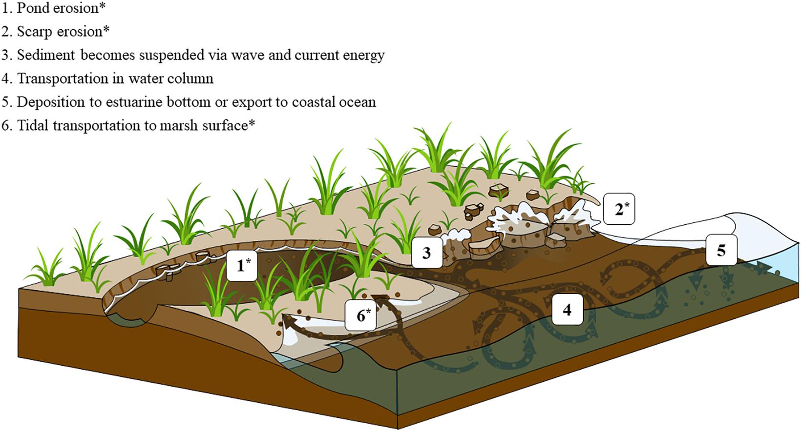
Figure 1. Conceptual figure depicting salt marsh carbon liberation and redistribution vectors. 1–2 illustrate processes that release buried sediment carbon from intact marshes. 3–6 show physical processes that move sediment to locations where decomposition can occur. This experiment mimics the conditions of wet sediment exposed to air, which occurs after either pond erosion (1) or edge erosion (2) and subsequent tidal trasport of eroded material to the sediment surface at either the erosion site or elsewhere (6). The decomposition of sediment suspended in the water column and transported away from the erosion site was not measured by this experiment.
In this study, we address what proportion of salt marsh belowground organic carbon will remineralize to CO2 or CH4 after an erosion event. Salt marsh erosion to oxic horizons was simulated by incubating sediment organic matter from two depths in oxic chambers at two different temperatures and directly measuring CO2 and CH4 production. We utilized these results to estimate the amount of belowground carbon released annually via shoreline erosion in the conterminous United States (CONUS). Because few experimental data exist to substantiate the current range of belowground organic carbon conversion to GHGs, this study provides empirical data to refine the range of potential emissions from the post-disturbance decomposition of salt marsh sediment carbon. These data will provide context for estimates of the effect of global warming on marsh C cycles.
Materials and Methods
Sample Collection
Replicate cores (n = 10) were collected from Freeman Creek marsh located on Marine Corps Base Camp Lejeune on the coast of North Carolina (34° 35.69′ N, 77° 15.12′ W). Cores were collected with a Russian peat corer (5 cm diameter) from a section of interior marsh dominated by Spartina alterniflora. Cores were collected at 0.062 m NAVD88 at the interface of short-form and tall-form S. alterniflora. Samples were transferred to PVC cradles and wrapped in cling wrap to minimize contact with air for transport to the NOAA lab in Beaufort, NC. 5 L of creek water (salinity = 32) was collected from the site.
Incubation Chamber Design
Decomposition incubations were designed to measure the production of CO2 and CH4 after simulated erosion of marsh sediment to oxygenated conditions (Supplementary Figure 2). 500 mL PETG (polyethylene terephthalate copolymer) bottles were used as incubation chambers due to their low CO2 permeability (8.06 cm3-mil/m2-24 h-atm). Each bottle was sealed with a Nalgene 38–430 cap with two 1/4–28 ports fitted with a polypropylene spin collar (Western Fluids Engineering, CA, United States). Each port was then fitted with a quick-connect coupling insert with matching threads and a valved shut-off system so that when the insert is not connected to its female counterpart, it is closed to air exchange (Part # PMCD24042812; Colder Products, MN, United States). Teflon tape was wrapped around the insert’s threads to ensure a tight fit. The mating part was a quick-connect coupling body (Part # PMC130412) with no valve, which was attached to the inlet and outlet of the greenhouse gas analyzer using 1/4-inch PTFE tubing. Without a valve, the inflow and outflow of air to the greenhouse gas analyzer was unimpeded when disconnected from the coupling counterpart. During the experiment, the cap ports were submerged in water further decreasing their chance of contamination with the ambient atmosphere. Chambers were wrapped in aluminum foil to ensure darkness during incubation.
Experimental Design
A 2-way factorial experiment was conducted testing the effect of temperature and sediment depth, a proxy for age and OM quality, on the decomposition rate of salt marsh sediment OM. Two 5-cm segments were cut from each replicate core and designated as shallow (5–10 cm below surface) or deep (20–25 cm below surface) sediment. The segment depths were decided after visual inspection of the cores confirmed the shallower depth material was situated in the rhizosphere while the latter was beneath the rhizosphere. The shallow and deep sections of wet sediment from all 10 cores were homogenized by hand for 5 min in a clean Ziploc bag before dividing ∼1 g wet weight of sediment into tared incubation chambers. Sediment wet weight was recorded. Two replicate aliquots were also prepared from each homogenized sample and placed in previously combusted (550°C) aluminum boats for subsequent analysis of water and organic carbon content.
Creek water was filtered with a 0.22 μm membrane filter. An inoculum of unfiltered creek water was reintroduced to the filtered water at a concentration of 6 mL L–1 after passing over 55 μm Nitex mesh to remove large particulates. To ensure that any microautotrophs present in the inoculate would not fix inorganic carbon during the incubation, diuron (3-(3,4-dichlorophenyl)-1,1-dimethylurea) was added to inhibit photosynthesis (Morin et al., 2018). Diuron is a common algicide that inhibits photosynthesis by specifically interrupting photosystem II but does not interrupt other metabolisms to our knowledge (Rutherford and Krieger-Liszkay, 2001). For every 1L of creek water, 60 μL of diuron solution (1.0134 g dissolved in 25 mL of 100% ethanol) was added. 3 mL of inoculated creek water was added to each incubation chamber and was shaken to mix with the sediment. Each chamber was sealed with the previously described 2-ported cap and submerged in an incubation bath at either 20 or 30°C. Replicate (n = 3) incubations were conducted simultaneously for each depth interval (shallow vs. deep) and temperature (20 vs. 30°C) for a total of 12 incubation chambers.
Greenhouse Gas Analysis
Concentrations of CO2 and CH4 were simultaneously measured in each incubation chamber using an ultra-portable greenhouse gas analyzer (GGA; Los Gatos Research, Inc., CA, United States). The GGA utilizes off-axis integrated cavity output spectroscopy to detect instantaneous gas concentrations at part-per-billion sensitivity. CO2 and CH4 production were measured as change in concentration over time. When the GGA is coupled to the incubation chamber by connecting its inlet and outlet ports to the chamber’s ported cap, a closed system is created. System equilibration occurred when the incubation chamber’s gas concentration homogenizes with the gases in the instrument’s headspace and a constant concentration reading is reported by the instrument. During the days between readings while the chamber was detached from the GGA, the port caps were sealed with closed valves and CO2 (and CH4) accumulated as respiration of OM occurred. To measure the concentration at the next time point, the GGA would again be connected to the chamber ports and the concentration of CO2 (and CH4) from the headspace inside the GGA would equilibrate with chamber gases.
The concentration of gases within the chamber (Cchamber) was derived from the equation
where V = headspace volume and C = gas concentration, GGA = the greenhouse gas analyzer, chamber = decomposition chamber, and TOTAL = chamber connected to the GGA by the inlet and outlet ports. This approach accounts for the CO2 and CH4 concentrations in the GGA volume prior to mixing with the decomposition chamber’s atmosphere. The Ideal Gas Law was assumed since temperature and pressure were known. This methodology of measuring gas accumulation also replenishes oxygen to the incubation chamber every time they were connected to the GGA ensuring oxic decomposition could continue. The incubation chamber was never less than 90% initial oxygen if we assumed the CO2 produced during incubation required an equal amount of oxygen using a 1:1 molar ratio.
Gas concentrations were measured approximately every 3 days for the initial 6 weeks of the incubation, after which measurements were less frequent at about once per week. After each measurement, the amount of C respired was subtracted from the available substrate. The experiment was maintained until all incubation chamber replicates from every treatment reached at least 4% loss of substrate, which occurred after 161 days. A reference gas mixture (402 ppmv CO2, 1.999 ppmv CH4; Scott-Marrin Inc., Riverside, CA) was measured periodically to ensure there was no drift in the instrument.
Elemental Analysis of Sediments
Representative aliquots (n = 4) of incubated sediment were used to estimate the initial carbon content in the wet sediment dispersed into each incubation chamber. Replicate sediment aliquots were dried to a constant weight at 60°C. Water content was measured as wet weight minus dry weight. Once dry, sediments were homogenized by hand with mortar and pestle and acidified with 0.1 M HCl. No bubbling was observed. A small subsample of each was weighed to the nearest 10–6 g and wrapped in a silver tin for elemental analysis (Costech ECS 4010). Internal acetanilide standards consistently produced a coefficient of variance less than 1.5%.
Calculating Decomposition Rates, Q10, and Activation Energy
Decomposition rate was calculated as the amount of CO2 produced per available OC substrate in a measured time interval, standardized as μmol C ⋅ mol C–1 ⋅ day–1. Q10 represents the temperature sensitivity for a reaction with a 10°C increase, defined as:
where Rw is the decomposition rate at the warmer temperature (in this case 30°C), Rc is the decomposition rate at the cooler temperature (in this case 20°C), and (Tw – Tc) is the difference between the two temperatures. As decomposition of OM occurs in sediment, the more labile fraction of OM might be consumed initially while less labile fractions within the same parcel of sediment take longer to decompose, which would bias Q10 over the duration of the experiment. The metric Q10–q developed by Conant et al. (2008) standardizes Q10 to substrate quality to ensure that Q10 is not influenced by changing lability of organic matter substrate. Following Conant et al. (2008), Q10–q was used to check if the changing quality of OM was a driver of differing decomposition rates by comparing the time required to decompose a fraction of OM at the cooler temperature (tc) to the time required to decompose that same fraction at the warmer temperature (tw), calculated as
If the decreasing quality of sediment substrate is affecting the decomposition rate, then tc should increase for later fractions of OM and cause Q10–q to increase.
To calculate activation energy (Ea), we used the form of the Arrhenius equation
where R is the gas constant (0.008314 kJ ⋅ K–1 ⋅ mol–1), k1 and k2 are rates of reactions at temperatures T1 and T2 in Kelvin. Once Ea was derived for the decomposition reaction for shallow and deep sediments, then the temperature-dependent rate (k2, or kT hereafter) at any temperature (T) could be determined using Ea and setting k1 to the rate at 20°C.
In situ Water Temperature Records for Site-Specific Decomposition
Water temperature time series data were gathered to apply the previously determined kT to in situ conditions in order to calculate site-specific, temperature-dependent decomposition rates. Long-term monitoring has produced continuous water temperature data from a tide gauge located in an estuarine embayment inside of the New River Inlet, approximately 8 km from where cores were collected. A 600LS data sonde (YSI Inc., OH, United States) was secured to a dock piling and recorded estuarine water temperature every 6 min. The temperature sensor utilizes a thermistor of sintered metallic oxide that changes predictably in resistance as temperature varies. The sonde was regularly checked every 1–2 months for fouling and battery life. Temperature was factory calibrated with an accuracy of ±0.15°C. Due to the proximity of sites adjacent to the New River Estuary, we assume the temperature at the monitoring station approximates the temperature distribution of the coring station.
Water temperature data from coastal states in the CONUS were gathered as well. Six-minute water temperature data from 171 NOAA Center for Operational Oceanographic Products and Services (CO-OPS) water level stations were downloaded using the R package rnoaa (Chamberlain, 2021). Of those, 155 stations met the requirements of containing a continuous 12-month period at least 95% temporally complete. 149 of those were >99% complete. Temperature was rounded to the nearest integer to sum temperature durations to derive k2 from Eq. (4) in subsequent calculations.
For our study site and each CO-OPS station, duration at each temperature was integrated with kT and summed to determine annual decomposition rates for each station (mol C ⋅ mol C–1, or %). Results from each station were standardized to annual rates by dividing the integrated sum by the proportion of record completeness. Applying the most-complete temperature record from each station regardless of start year or month effectively randomizes sampling date and ensures regional trends are not an ephemeral artifact of sampling period. A mean decomposition rate was determined for each state. Standard deviation of the mean state decomposition rate was calculated to represent variation of temperature records in each state.
C Emissions From Eroded Marsh Sediment in CONUS
In order to determine annual C emissions from decomposition of eroded salt marsh sediment, the previously determined average statewide decomposition rate was multiplied by the C in estimated eroded salt marsh sediment volume. Annual input (m3) of eroded marsh sediment was estimated by multiplying state-by-state estimates of marsh shoreline length by an estimate of horizontal annual erosion and vertical bank height (Currin et al., 2015). For all coastal states except Louisiana, we used marsh shoreline length from Gittman et al. (2015). A wide range in marsh shoreline has been reported for Louisiana, which we narrowed by extracting the ‘salt and brackish water marsh’ objects from the Louisiana Environmental Sensitivity Index (Office of Response and Restoration, 2020). For all marsh shorelines, we assumed an erosion rate of 0.3 m ⋅ yr–1 and a vertical bank height of 0.3 m, which fall within the low end of published values (Currin et al., 2015; Leonardi et al., 2016; Sapkota and White, 2019). A marsh sediment C density value of 27.0 kg ⋅ m–3 (Holmquist et al., 2018) was multiplied by erosion volume to determine the amount of marsh C liberated annually via bank erosion from shorelines. The amount of eroded marsh carbon was then multiplied by the average decomposition rate for each state to determine carbon emissions from eroded salt marsh. The kT experimentally determined for shallow sediment was applied to the top 0.1 m of the hypothetical 0.3 m tall erosional bank, while the kT determined for the deeper horizon from our experiment was applied to the sediment from 0.1 to 0.3 m. Raw data from the experiment and R scripts used for analysis are available in the Supplementary Material and at https://github.com/QAWalker/BlueCarbonErosionAndDecomp.
Results
Sediment Carbon Content
Sediment from the shallow (5–10 cm) horizon contained 11.9 ± 0.2 %OC, whereas sediment from the deep (20–25 cm) horizon contained 9.5 ± 0.1 %OC (Table 1). The molar C:N ratio for shallow and deep sediment horizons was 22.9 ± 0.8 and 21.4 ± 0.4, respectively. Decomposition rates were standardized to available carbon substrate, which differed in each treatment. The shallow sediment treatments contained 93.1 ± 5.6 mg C in the 20°C chambers and 89.0 ± 4.2 mg C in the 30°C chambers. The deep sediment treatment contained 128.6 ± 30.3 mg C in the 20°C chambers and 123.7 ± 6.9 mg C in the 30°C chambers.
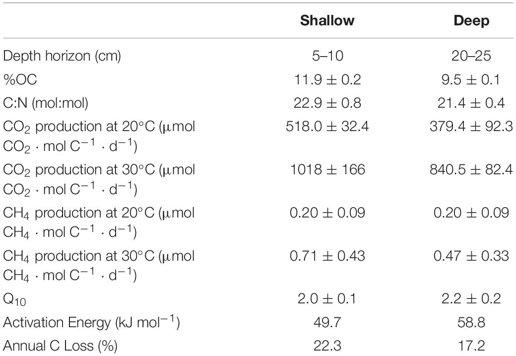
Table 1. Sediment characteristics and decomposition rates for the two experimental depth horizons.
Decomposition Rates
Over the course of the 161-day experiment, the CO2 production rates were relatively linear. By day 161, 8.4 ± 0.5% of the shallow sediment treatment at 20°C was respired. In the shallow treatment at 30°C, 16.4 ± 2.7% of the starting content was respired. The deep sediment horizon had lost 6.1 ± 1.5% and 13.5 ± 1.3% of available substrate at 20 and 30°C, respectively (Figure 2).
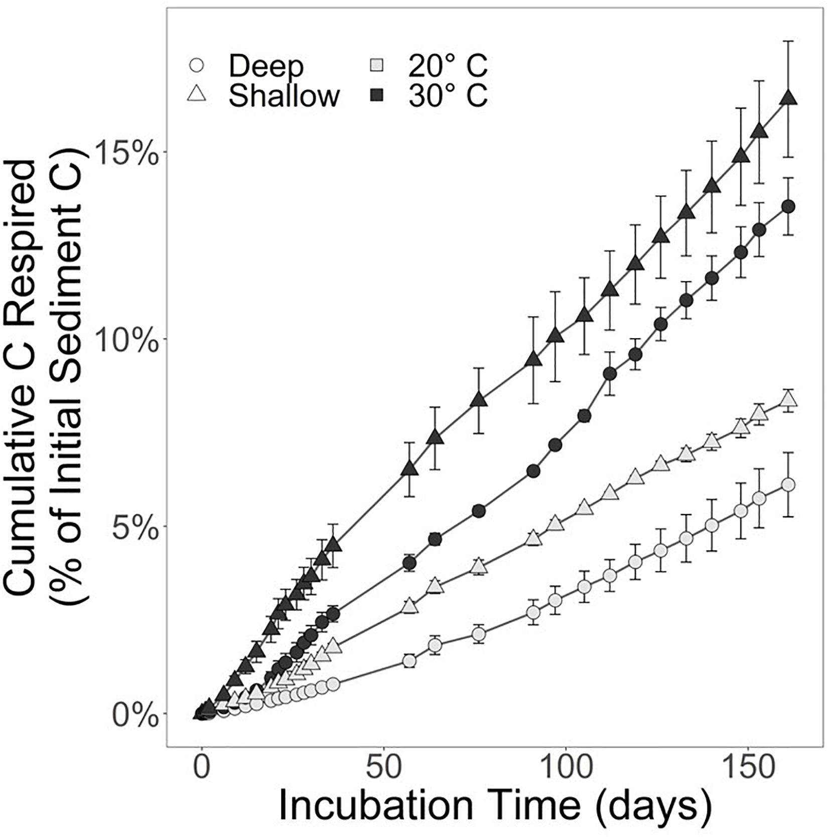
Figure 2. Substrate respired for the shallow sediment horizon (triangles) and deep sediment horizon (circles). The black markers represent the incubation held at 30°C, whereas light gray markers indicate the 20°C incubation. Error bars represent the standard error of the mean. Refer to Table 1 for CO2 and CH4 production rates.
The respiration rates at 30°C were faster than at 20°C for both sediment depth treatments (Figure 2). Moreover, the shallow sediment treatments at either temperature exhibited faster respiration rates than the deeper sediment treatments at either temperature. On average, the CO2 production rates for the shallow sediment treatments were 518.0 ± 32.4 and 1,018 ± 166 μmol CO2 ⋅ mol C–1 ⋅ d–1 for 20 and 30°C, respectively (Table 1). The CO2 production rates for the deep sediment treatments at 20 and 30°C were 379.4 ± 92.3 and 840.5 ± 82.4 μmol CO2 ⋅ mol C–1 ⋅ d–1, respectively.
CH4 was produced at detectable levels during the experiment, albeit at fractional concentrations compared to CO2 (Table 1). The shallow sediment treatments exhibited rates of CH4 production at 0.20 ± 0.09 and 0.71 ± 0.43 μmol CH4 mol C–1 ⋅ d–1 at 20 and 30°C, respectively. The deep sediment treatments evolved CH4 at rates of 0.20 ± 0.09 and 0.47 ± 0.33 μmol CH4 ⋅ mol C–1 ⋅ d–1 at 20 and 30°C, respectively.
Q10, Q10–q, and Ea
Q10 for OC loss from sediments as CO2 and CH4 production in shallow and deep sediment horizons was 2.0 ± 0.1 and 2.2 ± 0.2, respectively, for the entire course of the experimental incubation. Q10 between the depth horizons was not significantly different (p > 0.05). In order to account for the potential change in lability of decomposable substrate, Q10–q was determined for both sediment horizons (Figure 3). Q10–q in the shallow sediment horizon was 2.4 ± 0.2 for the first-1% of OC substrate remineralized compared to 2.1 ± 0.3 for the fifth-1%. For the deep sediment horizon, Q10–q decreased from 2.2 ± 0.2 to 1.3 ± 0.1 from the first-1% to the fifth-1% interval of substrate lost. The Ea for decomposition of sediment OM was 49.7 kJ ⋅ mol–1 for the shallow sediment horizon compared to the deeper sediment horizon at 58.8 kJ ⋅ mol–1 (Table 1).
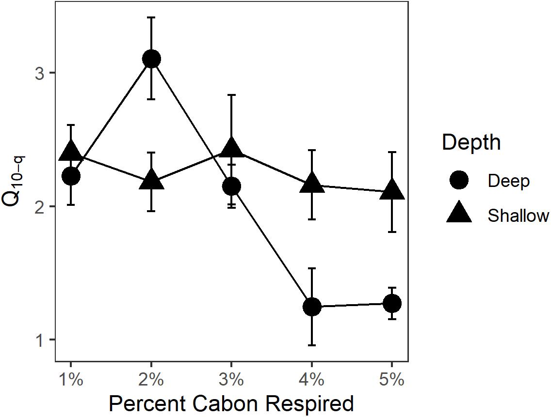
Figure 3. Q10–q for each percent of OC decomposed. As decomposition preferentially consumes labile fractions of available OC within the substrate, more refractory fractions remain and would potentially take longer to decompose. Since Q10–q did not increase over the course of the experiment, changing substrate quality over time was not an important factor regulating the decomposition process.
Site Decomposition Predicted by in situ Temperature
High-frequency (6-min) water temperature data from the study site collected over a year from April 2015 to March 2016 were employed to calculate annual decomposition rates of sediment OM using the respective Ea of shallow and deep sediment (Figure 4). The temperature-integrated annual decomposition rate for shallow sediment was 223 mmol C ⋅ mol C–1 ⋅ yr–1, or 22.3% (Figure 4; Table 1). Using the same annual temperature profile, the decomposition rate for the deeper sediment with a higher Ea was 172 mmol C ⋅ mol C–1 ⋅ yr–1, or 17.2%.
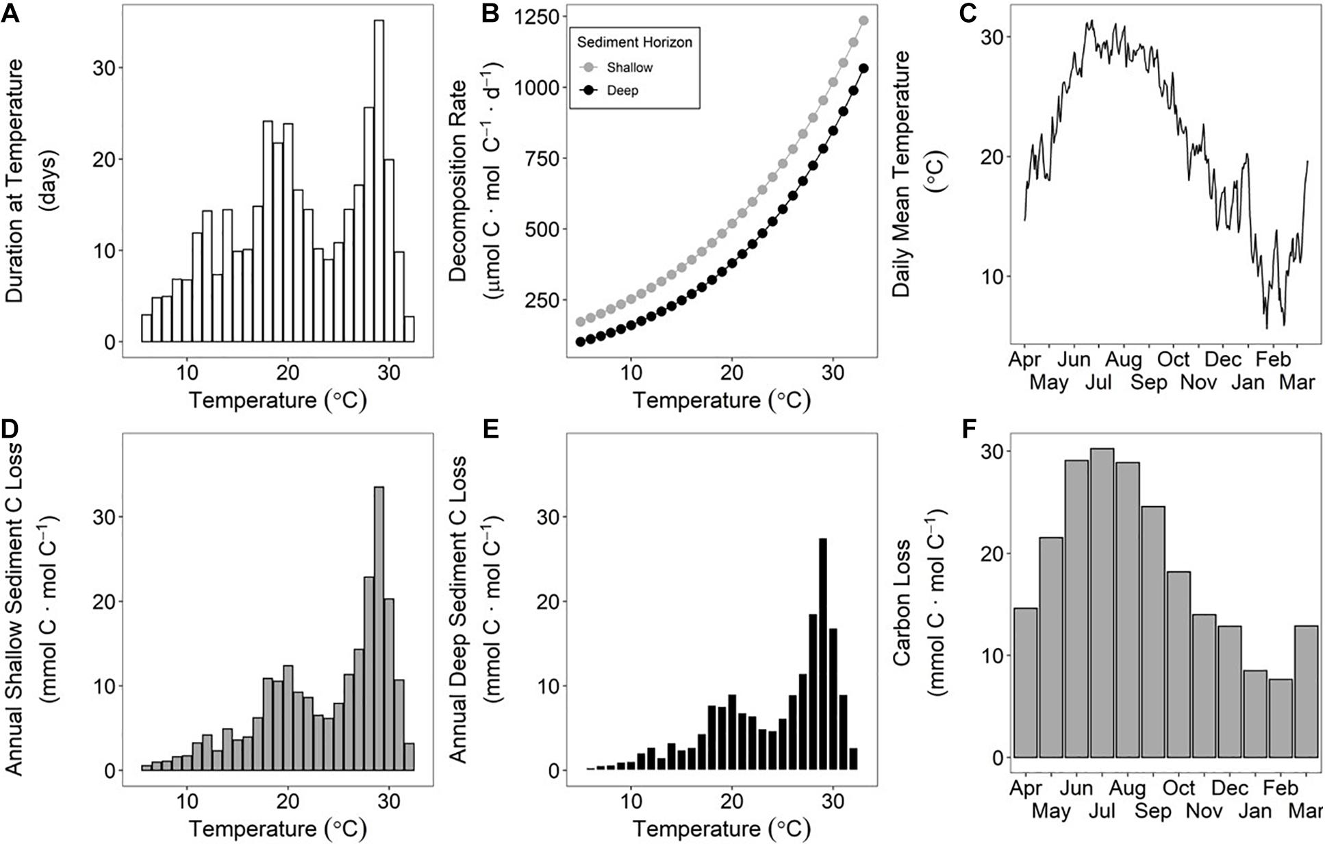
Figure 4. Study site temperature from April 2015 to March 2016 binned by 1°C and shown as frequency in days (A). The temperature-specific decomposition rates for each sediment horizon determined by Arrhenius kinetics (B). Time-series of daily mean temperature at study site (C). When the duration at a specific temperature (A) is multiplied by the temperature specific decomposition rate (B), then the sediment carbon loss at each temperature can be calculated for the shallow (D) and deep horizons (E). The sum of all bars in (D,E) is the annual decomposition rate for shallow and deep sediment horizons, respectively, or 223 and 172 mmol C ⋅ mol C–1 ⋅ yr–1. Note that 1 mmol C ⋅ mol C–1 = 0.1%. Monthly decomposition rates vary across the year (F), so the timing of erosion can be impactful on sub-annual exposure of OM to oxic horizons prior to reburial. The shallow horizon sediment was used in (F) for illustrative purposes.
Estimated GHG Emissions From Eroded Marsh Sediment in CONUS
Salt marsh shorelines in the CONUS erode an estimated sediment volume of 12.81 × 10⁶ m3 ⋅ yr–1 (Table 2). The majority (>96%) of this occurs in the Atlantic and Gulf of Mexico regions where most of the salt marsh in the CONUS exists. Annual erosion yields an estimated 345.9 Gg C liberated from intact salt marsh banks each year resulting in potential greenhouse gas emissions of 62.90 ± 2.81 Gg C ⋅ yr–1 from decomposition processes in dark, oxic conditions. A latitudinal gradient was produced where southern states exhibited higher decomposition rates (>20%) than those with more northern or Pacific Ocean coasts (Figure 5). Despite long coastlines, the states along the Pacific Ocean have relatively small amounts of salt marsh shoreline and cooler water year-round resulting in low amounts of eroded C (<4% of CONUS total) and C emissions (<2% of CONUS total) (Table 2).
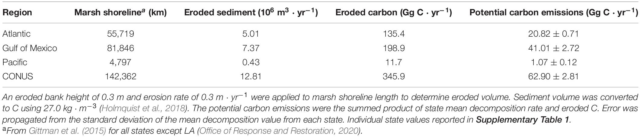
Table 2. Summary of erosion and subsequent potential C emissions from CONUS.
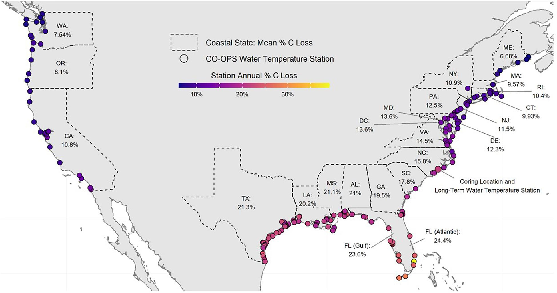
Figure 5. Map of calculated annual eroded marsh carbon loss at each coastal NOAA CO-OPS water temperature station in the Conterminous United States (CONUS). Each station denoted by a circle is an active NOAA CO-OPS temperature station colored by the amount of temperature-dependent decomposition (% loss per year) expected from eroded salt marsh. Statewide percentages are mean decomposition for all the CO-OPS stations in the state and calculated for a bank composed of 1/3 shallow sediment and 2/3 deep sediment. Florida stations were divided into Gulf and Atlantic regions following Gittman et al. (2015). The enlarged circle in NC indicates the location of the long-term temperature monitoring station located 8 km from the coring location.
Discussion
The Role of Temperature in Wetland OM Decomposition
Temperature rather than organic content and C:N played the larger role in regulating salt marsh sediment organic matter decomposition because the warmer treatments of both sediment horizons decomposed faster than the lower temperature treatments (Figure 2). Unlike decomposition experiments that use fresh OM to simulate the fate of recently deposited materials, this experiment utilized portions of the sediment carbon pool considered “stored” and not available for decomposition under undisturbed circumstances. These materials did not exhibit the classic exponential decay of fresh OM (e.g., Benner et al., 1991; Conant et al., 2008), but rather established a roughly linear decomposition rate from the experiment’s onset (Figure 2). The initial rapid decomposition associated with fresher OM is attributed to the preferential microbial remineralization of the more labile components before the portion of OM that is more resistant to microbial enzymatic breakdown is all that remains (Benner et al., 1991). After the labile fractions have been lost, there is a relatively slower, linear remineralization phase. Decomposition occurs in multiple phases because sediment OM consists of more than one-pool (Davidson et al., 2000). For the context of decomposition experiments, three-pools of sediment organic carbon exist with distinct lability and response to temperature: one fraction is labile, one is more resistant to degradation but will slowly remineralize, and the third is stable over the timescales that incubation experiments operate (Knorr et al., 2005). One explanation for the trend observed during this experiment is that the labile fraction of the sediment OM in both horizons had been remineralized prior to our collection and subsequent incubation. Therefore, decomposition rates shown here are for the more stable components of sediment OM, and notably, there was no reactive, quickly degrading fraction in the stored salt marsh sediment obtained from the cores, even at the 5–10 cm interval below the surface. This is further supported by the lack of increase in Q10–q over the course of the experiment (Figure 3). An increase in Q10–q over the incubation period would indicate that over time the quality of substrate is changing due to labile fractions preferentially being remineralized earlier in the incubation, and the less labile fractions taking longer to decompose later in the experiment (Conant et al., 2008, 2011). Contrary to this expectation, the slight decrease in Q10–q reflects that decomposition rates were slowest at the beginning of the incubation. This could be caused by the microbial community in the lower temperature incubations for both sediment horizons taking longer to achieve maximum respiration rates.
Apart from temperature or substrate quality, other factors, such as mineral protection, water content, redox zonation, and plant-microbe interactions are important factors that determine the decomposition of wetland OM (Dungait et al., 2012; Reynolds et al., 2017; Spivak et al., 2019). These factors no doubt regulate the accumulation and loss of OM in wetland sediments but might operate more prominently within intact sediments. Our experimental design controlled some of these factors by homogenizing the microbial community from the water column and conducting oxic incubations as the intent was to simulate erosion from an intact marsh. The incubated sediments were also physically homogenized and spread thin to maximize oxygenation and contact with microbes. Moreover, mineral protection of organic matter contained in the sediment matrix is likely a prominent factor that causes differences in decomposition rates between the incubation of homogenized sediment vs. plant biomass (Craine et al., 2010; Dungait et al., 2012).
We presume the deeper horizon contained older OM. Using a 210Pb geochronology for salt marsh cores near our study site within a similar elevation range -0.159 to 0.128 m NAVD88, McKee et al. (2018) derived a mean (±standard deviation) sediment accretion rate of 2.4 ± 0.9 mm ⋅ yr–1 using the Constant Flux model and 2.7 ± 1.4 mm ⋅ yr–1 using the Constant Flux Constant Sedimentation model. These rates fall on the low end of shorter-term measures of marsh surface elevation change measured at nearby S. alterniflora marshes of 2–12 mm ⋅ yr–1 (Davis et al., 2017), and are consistent with reduced sediment accretion at higher elevation, interior marshes. Assuming these rates determined by the 210Pb geochronology encompass the sediment accretion rate experienced at the coring location for this study, the shallow horizon age was between 19 to 42 years old before collection while the deeper horizon was between 74 to 104 years old before collection. The deeper, older horizon of sediment was respired slower compared to the shallower horizon at either temperature for the entire duration of the experiment, but there is not a dramatic difference between the chemical composition of the two horizons. Carbon content was slightly higher in the shallow horizon (11.9 ± 0.2%) vs. the deeper horizon (9.5 ± 0.1%), but the molar C:N ratios were similar (22.9 ± 0.8 vs. 21.4 ± 0.4 for shallow and deep, respectively), suggesting that the sediment OM pools were similar (Table 1). The sediment accretion rate could be conservative for estimating OM age since “pre-aged” material eroded from the marsh edge can be deposited on the marsh platform and reincorporated into marsh sediment (Canuel et al., 2009; Hopkinson et al., 2018; Figure 1). The “pre-aging” of the material incorporated into the sediment matrix could explain the similarity in chemical composition between the two horizons since they might contain OM of the age. Still, these results reveal a paradox of similar chemical character yielding different decomposition rates. The coarse elemental analysis conducted here does not provide the resolution required to elucidate the character of the more reactive shallower treatment other than demonstrating a slightly higher carbon content. Moreover, the conundrum of both sediment horizons exhibiting no detectable difference in quality precluded us from the testing the CQT hypothesis directly. The sediment horizons exhibited similar temperature sensitivity (i.e., similar Q10) albeit at different respiration rates due to the different Ea measured for each horizon.
The temperature sensitivity of salt marsh OM has implications in scaling up our results to landscape or regional climate models and would have a positive feedback on CO2-induced warming since the deeper (>0.1 m) sediment that acts as a carbon reservoir prior to erosion becomes an increasing source of GHGs as it experiences warmer temperatures post-erosion. To demonstrate this concept, we will use a hypothetical incubation chamber comprised of equal parts of the two depth horizons used in this experiment that continue to exhibit consistent decomposition rates presented above. At 5°C the decomposition rate would total 137 μmol CO2 ⋅ mol C–1 ⋅ d–1 of which 63% of the CO2 is from the shallow pool and 37% is from the deep (Figure 6). However, at 30°C the total decomposition increases to 933 μmol CO2 ⋅ mol C–1 ⋅ d–1 but the proportion of decomposition changes to 55% and 45% for shallow and deep fractions, respectively. Given the continued disturbance of wetlands via erosion (Leonardi et al., 2016; Sapkota and White, 2019; Donatelli et al., 2020), sea-level rise (FitzGerald and Hughes, 2019), and eutrophication (Deegan et al., 2012), a large portion of the presently stable deeper horizons of wetland sediment could be remineralized to CO2. Our experiment was conducted under conditions similar to those of marsh sediment exposed to the atmosphere, which occurs during low tides. When decomposition occurs while the marsh sediment is submerged or after tidal flushing of pore spaces, CO2 from marsh decomposition enters the DIC pool and can be advected into estuarine and coastal ocean waters where it could exchange with the atmosphere or become retained in deeper waters (Wang et al., 2016; Maher et al., 2018; Najjar et al., 2018).
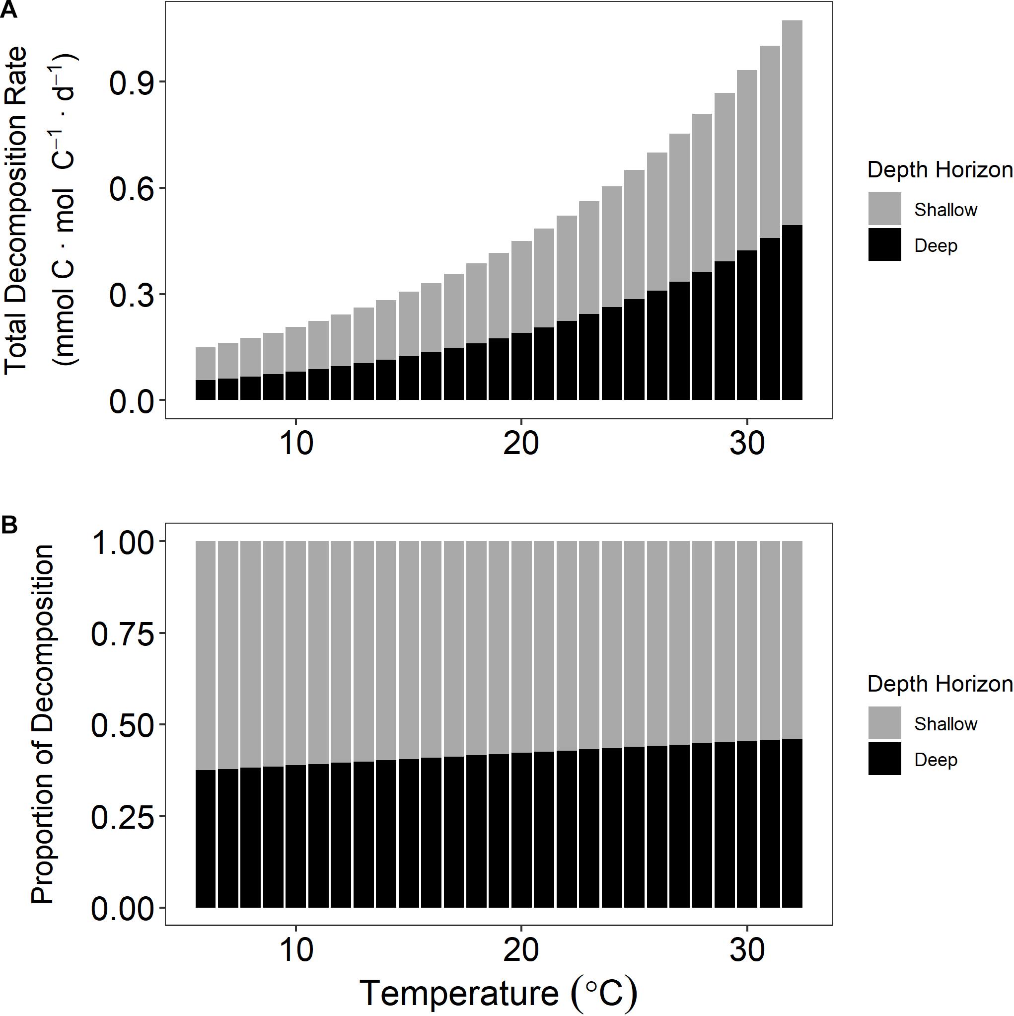
Figure 6. Decomposition rate at multiple temperatures for a hypothetical incubation chamber that contained equal parts of both sediment horizons. Total decomposition rate increases with temperature (A). The proportional contribution of the deep horizon that possesses a higher activation energy (Ea) increases with temperature (B).
While the initial transport of eroded material can be to oxygenated settings, including the salt marsh surface and water column (Hopkinson et al., 2018), eventually most of that material is reburied into anoxic sediment horizons where oxic breakdown will halt (Figure 1). Since oxic decomposition will not likely continue indefinitely, the timing and frequency of the erosion event is an important consideration for decomposition of material that remains in an oxic environment less than a year. At the North Carolina coring site, if salt marsh was hypothetically eroded in April but reburied 6 months later, it would experience the highest temperatures of the year and decompose with correspondingly higher rates (Figures 4C,F). Comparatively, material eroded in October and reburied 6 months later would experience the colder winter temperatures and decompose approximately half that of what would have occurred in the previous 6 months.
OC accumulation in wetlands occurs, in part, due to the anoxic state of their waterlogged sediments. Phenolic compounds (e.g., lignin) that are integral to the physical structure of vascular plants can resist decomposition within wetland sediments since the enzyme phenol oxidase required to breakdown phenolic compounds requires oxygen (Janusz et al., 2017). Therefore, the oxygenation of wetland sediment upon disturbance (e.g., wetland erosion or drainage) can unfasten the enzymatic “latch” that preserves stored belowground OM from remineralization to CO2 (Freeman et al., 2001). A portion of the CO2 flux we measured could be from lignin and other phenolic compounds that were previously stored in the sediments unable to degrade prior to the simulated erosion. We note that our results are specific to salt marsh sediments that have been oxygenated.
We measured small fluxes of CH4 production, an anaerobic process, despite the oxic and near-ocean salinity conditions of the experiment. This suggests that anoxic microsites formed within the sediment matrix of the experimental substrate (Ribas et al., 2019). CH4 is a more potent greenhouse gas than CO2 with a 100-year global warming potential (GWP) of 28 (Boucher et al., 2009). Considering this factor, the daily CH4 production was still dwarfed by the CO2 production. For example, in the shallow sediment incubation at 30°C, there was still 51 times more CO2 production than GWP-standardized CH4 production. Using oxygen to respire sediment carbon yields far more energy than methanogenesis, so these proportions are not surprising. However, it should be noted that even in an oxygenated, saline experimental setting, detectable amounts of CH4 were produced, which further supports that environmental factors cannot always predict methane emission (Al-Haj and Fulweiler, 2020). Given that methanogenesis occurred during the incubation, other anaerobic processes like sulfate reduction or denitrification may have occurred as well until the terminal electron acceptors for those processes were exhausted.
It should be noted that sediments with inorganic carbon constituents (e.g., oyster reefs, seagrass beds, coral reefs, etc.) would require additional consideration if used in this experimental design. Since a high CO2 atmosphere forms in the decomposition chambers, porewater pH would decrease along with aragonite saturation. As carbonate minerals dissolve, some CO2 would be consumed altering the measurable respiration. A high CO2 headspace and, thus, a low pH porewater could impact microbial activity as well; however, this was unmeasured in our study. The relatively linear rates of CO2 production do not suggest there were intermittent interruptions in microbial performance (Figure 2).
Refining Estimates of Carbon Emissions Post-disturbance Through Extrapolation
Extrapolated decomposition rates throughout CONUS were not an exact linear function of salt marsh shoreline due to regionally different temperature regimes. For example, North Carolina, South Carolina, and the Gulf Coast of Florida erode less C each year than Maryland, but each has higher total C emissions from decomposition since their coastal waters are warmer (Supplementary Table 1). Louisiana, with the longest marsh shoreline tallied here, erodes almost seven times more C annually than Virginia with the next longest marsh shoreline, but the warmer temperatures in Louisiana account for almost 10 times the C emissions.
The calculations conducted for this study are conservative for several reasons. The decomposition rates assume no photo-oxidation takes place, which most likely would take place in situ and would increase the decomposition rate (Wang et al., 2020). The introduction of sediment into a nutrient-rich water column may prime the microbial community and enhance decomposition (Ward et al., 2016; Bulseco et al., 2019). The rates reported here are specifically microbial respiration, and decomposition rates could potentially be higher in situ in the presence of grazers and detritivores. Our estimate also does not include additional losses that take place after habitat disturbance, as loss of salt marsh plants via erosion results in the loss of additional plant carbon fixation via photosynthesis or facilitation of sedimentation and subsequent burial of carbon. The experimentally determined decomposition rates exhibited variation of about 10%, which was not propagated into the state-by-state C emission rates. Lastly, tidal creeks where salt marshes exist can experience warmer temperatures than NOAA CO-OPS tide gauges, which are often located closer to the coastal ocean; therefore, the state-by-state decomposition estimates may be conservative. Despite these limitations, the decomposition rates extrapolated to CONUS provide context to previous estimates of C emissions.
Previous studies that estimate C emissions from salt marsh loss have been forced to make assumptions about decomposition rates due to the lack of empirical data that track the fate of sediment organic carbon to GHGs after habitat loss. Pendleton et al. (2012) estimated between 0.2 and 0.24 Pg C ⋅ yr–1 of global C emissions from salt marshes after land-use change or habitat loss. Their emission rates were broadly bounded with decomposition rates ranging between 25 and 100%. Similarly, Sapkota and White (2019) estimated C emissions from eroded salt marsh from Barataria Basin, LA, assuming a decomposition rate of 75% loss of sediment organic carbon. Conversely, our estimates for salt marsh sediment organic matter decomposition throughout CONUS range from 7 to 24% annual loss, which accounts for in situ temperature of the environments into which salt marsh OM is eroded. We assumed that Ea remains unchanged for 1 year to facilitate our calculation of an annual decomposition rate, but our laboratory measurements of GHG production lasted for only 161 days. It is possible that the rates would slow as decomposition progresses, thus, increasing Ea over the time during which the OM can decompose (Conant et al., 2008). For this reason, it is unrealistic to extrapolate these rates over a time frame required to reach 100% loss of OM. For example, while we report a mean state decomposition rate for Texas at ∼20% ⋅ yr–1, it is not implied that eroded salt marsh OM will completely decompose in 5 years. Moreover, a major question remains unanswered that is required to understand the long-term fate of eroded materials: will the eroded salt marsh OM remain in oxic conditions indefinitely or might they eventually become reburied? Evidence that eroded marsh edge OM is deposited on the marsh platform and reburied suggests that there is a finite time during which aerobic decomposition can take place (Hopkinson et al., 2018; Figure 1). We used the utility of reporting rates as per year; however, this does not imply the duration of decomposition of disturbed sediment in situ. One approach to estimate the anoxic duration would be to divide the depth that the anoxic zone in the marsh sediment begins by the sediment accretion rate if both were known.
The estimated rates of C emissions from eroded salt marsh were calculated with several caveats. We assumed all salt marsh decomposition occurs with the same Ea as measured in the laboratory experiment. It is plausible that Ea differs geographically as emergent vegetation and soil types change (Craine et al., 2010). Two states (SC and GA) had only one CO-OPS station that met our requirements; in these cases, the entire state’s salt marsh C emissions depended on the temperature record from one location. The decomposition calculation also hinges on quantifying salt marsh length. As this value becomes more accurately measured over time, especially in states with extensive wetlands like Louisiana, the estimate for decomposition from salt marshes will too refine. We also used a conservative, fixed bank height and erosion rate for the entire CONUS, but these vary spatially as they are dependent on a multitude of hydrographic, morphologic, and chemical variables. Opting for lower erosion rates also helps balance the occurrence of prograding and non-eroding marsh shorelines. This extrapolation exercise is one example of an application for measuring temperature-based decomposition rates of coastal sediment organic matter to predict future GHG emission scenarios. Blue carbon ecosystems are renowned for their abilities to accrete and store carbon but refining how losses to their extent feed a positive GHG feedback loop is essential to understanding their full value.
Data Availability Statement
The original contributions presented in the study are included in the article/Supplementary Material, and further inquiries can be directed to the corresponding author.
Author Contributions
NM and CC conceived and designed the experiment. NM, QW, and CC collected, analyzed, and interpreted the data. NM and QW generated the tables and figures. NM wrote the manuscript with input, guidance, and revisions from QW and CC. All authors contributed to the article and approved the submitted version.
Funding
This research was conducted under the Defense Coastal/Estuarine Research Program (DCERP), funded by the Strategic Environmental Research and Development Program (SERDP).
Disclaimer
The scientific results and conclusions, as well as any views or opinions expressed herein, are those of the authors and do not necessarily reflect the views of NOAA or the Department of Commerce and should not be construed as an official U.S. Department of Defense position or decision unless so designated by other official documentation.
Conflict of Interest
QW was employed by the company CSS-Inc.
The remaining authors declare that the research was conducted in the absence of any commercial or financial relationships that could be construed as a potential conflict of interest.
Acknowledgments
We thank E. Canuel and B. Puckett for their helpful comments during internal peer review. R. Gianelli assisted with laboratory analysis and field collection. This research was performed while NM held a National Research Council Research Associateship award at the NOAA National Centers for Coastal Ocean Science.
Supplementary Material
The Supplementary Material for this article can be found online at: https://www.frontiersin.org/articles/10.3389/fmars.2021.661442/full#supplementary-material
References
Al-Haj, A. N., and Fulweiler, R. W. (2020). A synthesis of methane emissions from shallow vegetated coastal ecosystems. Glob. Change Biol. 26, 2988–3005. doi: 10.1111/gcb.15046
Benner, R., Fogel, M., and Sprague, E. (1991). Diagenesis of belowground biomass of spartina alterniflora in salt-marsh sediments. Limnol. Oceanogr. 36, 1358–1374. doi: 10.4319/lo.1991.36.7.1358
Bosatta, E., and Ågren, G. I. (1999). Soil organic matter quality interpreted thermodynamically. Soil Biol. Biochem. 31, 1889–1891. doi: 10.1016/S0038-0717(99)00105-4
Boucher, O., Friedlingstein, P., Collins, B., and Shine, K. P. (2009). The indirect global warming potential and global temperature change potential due to methane oxidation. Environ. Res. Lett. 4:044007. doi: 10.1088/1748-9326/4/4/044007
Brevik, E. C., and Homburg, J. A. (2004). A 5000 year record of carbon sequestration from a coastal lagoon and wetland complex, Southern California, USA. CATENA 57, 221–232. doi: 10.1016/j.catena.2003.12.001
Bulseco, A. N., Giblin, A. E., Tucker, J., Murphy, A. E., Sanderman, J., Hiller−Bittrolff, K., et al. (2019). Nitrate addition stimulates microbial decomposition of organic matter in salt marsh sediments. Global Change Biol. 25, 3224–3241. doi: 10.1111/gcb.14726
Campbell, A., Lera, M., Igor, L., Holly, G., and Adam, H. (2008). Carbon Storage in Protected Areas: Technical Report.
Canuel, E. A., Lerberg, E. J., Dickhut, R. M., Kuehl, S. A., Bianchi, T. S., and Wakeham, S. G. (2009). Changes in sediment and organic carbon accumulation in a highly-disturbed ecosystem: the Sacramento-San Joaquin River Delta (California, USA). Mar. Pollut. Bull. 59, 154–163. doi: 10.1016/j.marpolbul.2009.03.025
Chamberlain, S. (2021). rnoaa: ‘NOAA’ Weather Data from R. R package version 1.3.2. Available online at: https://CRAN.R-project.org/package=rnoaa
Chapman, S. K., Hayes, M., Kelly, B., and Langley, J. A. (2019). Exploring the oxygen sensitivity of wetland soil carbon mineralization. Biol. Lett. 15:407. doi: 10.1098/rsbl.2018.0407
Conant, R. T., Drijber, R. A., Haddix, M. L., Parton, W. J., Paul, E. A., Plante, A. F., et al. (2008). Sensitivity of organic matter decomposition to warming varies with its quality: temperature sensitivity of organic matter decomposition. Glob. Change Biol. 14, 868–877. doi: 10.1111/j.1365-2486.2008.01541.x
Conant, R. T., Ryan, M. G., Ågren, G. I., Birge, H. E., Davidson, E. A., Eliasson, P. E., et al. (2011). Temperature and soil organic matter decomposition rates – synthesis of current knowledge and a way forward. Glob. Change Biol. 17, 3392–3404. doi: 10.1111/j.1365-2486.2011.02496.x
Craine, J. M., Fierer, N., and McLauchlan, K. K. (2010). Widespread coupling between the rate and temperature sensitivity of organic matter decay. Nat. Geosci. 3, 854–857. doi: 10.1038/ngeo1009
Currin, C., Davis, J., Baron, L. C., Malhotra, A., and Fonseca, M. (2015). Shoreline change in the New River Estuary, North Carolina: rates and consequences. J. Coast. Res. 315, 1069–1077. doi: 10.2112/JCOASTRES-D-14-00127.1
Davidson, E. A., and Janssens, I. A. (2006). Temperature sensitivity of soil carbon decomposition and feedbacks to climate change. Nature 440, 165–173. doi: 10.1038/nature04514
Davidson, E. A., Trumbore, S. E., and Amundson, R. (2000). Soil warming and organic carbon content. Nature 408, 789–790. doi: 10.1038/35048672
Davis, J., Currin, C., and Morris, J. T. (2017). Impacts of fertilization and tidal inundation on elevation change in microtidal, low relief salt marshes. Estuar. Coasts 40, 1677–1687. doi: 10.1007/s12237-017-0251-0
Deegan, L. A., Johnson, D. S., Warren, R. S., Peterson, B. J., Fleeger, J. W., Fagherazzi, S., et al. (2012). Coastal eutrophication as a driver of salt marsh loss. Nature 490, 388–392. doi: 10.1038/nature11533
Donatelli, C., Zhang, X., Ganju, N. K., Aretxabaleta, A. L., Fagherazzi, S., and Leonardi, N. (2020). A nonlinear relationship between marsh size and sediment trapping capacity compromises salt marshes’ stability. Geology 48, 966–970. doi: 10.1130/G47131.1
Dungait, J. A. J., Hopkins, D. W., Gregory, A. S., and Whitmore, A. P. (2012). Soil organic matter turnover is governed by accessibility not recalcitrance. Glob. Change Biol. 18, 1781–1796. doi: 10.1111/j.1365-2486.2012.02665.x
Fagherazzi, S., Mariotti, G., Wiberg, P., and McGlathery, K. (2013). Marsh collapse does not require sea level rise. Oceanography 26, 70–77. doi: 10.5670/oceanog.2013.47
FitzGerald, D. M., and Hughes, Z. (2019). Marsh processes and their response to climate change and sea-level rise. Annu. Rev. Earth Planet. Sci. 47, 481–517. doi: 10.1146/annurev-earth-082517-010255
Freeman, C., Ostle, N., and Kang, H. (2001). An enzymic “latch” on a global carbon store. Nature 409, 149–149. doi: 10.1038/35051650
Ganju, N. K., Defne, Z., and Fagherazzi, S. (2020). Are elevation and open-water conversion of salt marshes connected? Geophys. Res. Lett. 47:e2019GL086703. doi: 10.1029/2019GL086703
Gedan, K. B., Silliman, B. R., and Bertness, M. D. (2009). Centuries of human-driven change in salt marsh ecosystems. Ann. Rev. Mar. Sci. 1, 117–141. doi: 10.1146/annurev.marine.010908.163930
Gittman, R. K., Fodrie, F. J., Popowich, A. M., Keller, D. A., Bruno, J. F., Currin, C. A., et al. (2015). Engineering away our natural defenses: an analysis of shoreline hardening in the US. Front. Ecol. Environ. 13:301–307. doi: 10.1890/150065
Holmquist, J. R., Windham-Myers, L., Bliss, N., Crooks, S., Morris, J. T., Megonigal, J. P., et al. (2018). Accuracy and Precision of Tidal Wetland Soil Carbon Mapping in the Conterminous United States. Sci. Rep. 8:9478. doi: 10.1038/s41598-018-26948-7
Hopkinson, C. S., Morris, J. T., Fagherazzi, S., Wollheim, W. M., and Raymond, P. A. (2018). Lateral marsh edge erosion as a source of sediments for vertical marsh accretion. J. Geophys. Res. Biogeosci. 123, 2444–2465. doi: 10.1029/2017JG004358
Janusz, G., Pawlik, A., Sulej, J., Świderska-Burek, U., Jarosz-Wilkołazka, A., and Paszczyński, A. (2017). Lignin degradation: microorganisms, enzymes involved, genomes analysis and evolution. FEMS Microbiol. Rev. 41, 941–962. doi: 10.1093/femsre/fux049
Johnson, B. J., Moore, K. A., Lehmann, C., Bohlen, C., and Brown, T. A. (2007). Middle to late holocene fluctuations of C3 and C4 vegetation in a northern New England salt marsh, Sprague marsh, Phippsburg, Maine. Organic Geochem. 38, 394–403. doi: 10.1016/j.orggeochem.2006.06.006
Knorr, W., Prentice, I. C., House, J. I., and Holland, E. A. (2005). Long-term sensitivity of soil carbon turnover to warming. Nature 433, 298–301. doi: 10.1038/nature03226
Le Quéré, C., Andrew, R. M., Friedlingstein, P., Sitch, S., Hauck, J., Pongratz, J., et al. (2018). Global carbon budget 2018. Earth Syst. Sci. Data 10, 2141–2194. doi: 10.5194/essd-10-2141-2018
Leonard, L. A., and Croft, A. L. (2006). The effect of standing biomass on flow velocity and turbulence in Spartina alterniflora canopies. Estuar. Coast. Shelf Sci. 69, 325–336. doi: 10.1016/j.ecss.2006.05.004
Leonardi, N., Ganju, N. K., and Fagherazzi, S. (2016). A linear relationship between wave power and erosion determines salt-marsh resilience to violent storms and hurricanes. Proc. Natl. Acad. Sci. U.S.A. 113, 64–68. doi: 10.1073/pnas.1510095112
Lovelock, C. E., Atwood, T., Baldock, J., Duarte, C. M., Hickey, S., Lavery, P. S., et al. (2017). Assessing the risk of carbon dioxide emissions from blue carbon ecosystems. Front. Ecol. Environ. 15:257–265. doi: 10.1002/fee.1491
Macreadie, P. I., Anton, A., Raven, J. A., Beaumont, N., Connolly, R. M., Friess, D. A., et al. (2019). The future of blue carbon science. Nat. Commun. 10:3998. doi: 10.1038/s41467-019-11693-w
Macreadie, P. I., Hughes, A. R., and Kimbro, D. L. (2013). Loss of ‘Blue Carbon’ from coastal salt marshes following habitat disturbance. PLoS One 8:e69244. doi: 10.1371/journal.pone.0069244
Maher, D. T., Call, M., Santos, I. R., and Sanders, C. J. (2018). Beyond burial: lateral exchange is a significant atmospheric carbon sink in mangrove forests. Biol. Lett. 14:20180200. doi: 10.1098/rsbl.2018.0200
Mariotti, G., and Carr, J. (2014). Dual role of salt marsh retreat: long-term loss and short-term resilience. Water Resour. Res. 50, 2963–2974. doi: 10.1002/2013WR014676
McKee, B., Bost, M., Atencio, A., Rodriguez, A., Currin, C., McTigue, N., et al. (2018). “Carbon burial in estuarine, wetland, and coastal barrier environments,” in Defense Coastal/Estuarine Research Program 2 Final Report, ed. P. Cunningham (Durham, NC: RTI International).
McTigue, N., Davis, J., Rodriguez, A. B., McKee, B., Atencio, A., and Currin, C. (2019). Sea level rise explains changing carbon accumulation rates in a salt marsh over the past two millennia. J. Geophys. Res. Biogeosci. 124, 2945–2957. doi: 10.1029/2019JG005207
Möller, I., Spencer, T., French, J. R., Leggett, D. J., and Dixon, M. (1999). Wave transformation over salt marshes: a field and numerical modelling study from North Norfolk, England. Estuar. Coastal Shelf Sci. 49, 411–426. doi: 10.1006/ecss.1999.0509
Morin, S., Chaumet, B., and Mazzella, N. (2018). A time-dose response model to assess diuron-induced photosynthesis inhibition in freshwater biofilms. Front. Environ. Sci. 6:131. doi: 10.3389/fenvs.2018.00131
Mudd, S. M., D’Alpaos, A., and Morris, J. T. (2010). How does vegetation affect sedimentation on tidal marshes? Investigating particle capture and hydrodynamic controls on biologically mediated sedimentation. J. Geophys. Res. 115:1566. doi: 10.1029/2009JF001566
Najjar, R. G., Herrmann, M., Alexander, R., Boyer, E. W., Burdige, D. J., Butman, D., et al. (2018). Carbon budget of tidal wetlands, estuaries, and shelf waters of eastern north America. Glob. Biogeochem. Cycle 32, 389–416. doi: 10.1002/2017GB005790
Office of Response and Restoration (2020). Louisiana and Lower Mississippi River 2014 ESIL (Environmental Sensitivity Index – Lines) from 2010-06-15 to 2010-08-15. Available online at: https://www.fisheries.noaa.gov/inport/item/53935 (accessed October 7, 2020).
Pendleton, L., Donato, D. C., Murray, B. C., Crooks, S., Jenkins, W. A., Sifleet, S., et al. (2012). Estimating global “Blue Carbon” emissions from conversion and degradation of vegetated coastal ecosystems. PLoS One 7:e43542. doi: 10.1371/journal.pone.0043542
Reynolds, L. L., Lajtha, K., Bowden, R. D., Johnson, B. R., and Bridgham, S. D. (2017). The carbon quality-temperature hypothesis does not consistently predict temperature sensitivity of soil organic matter mineralization in soils from two manipulative ecosystem experiments. Biogeochemistry 136, 249–260. doi: 10.1007/s10533-017-0384-z
Ribas, A., Mattana, S., Llurba, R., Debouk, H., Sebastià, M. T., and Domene, X. (2019). Biochar application and summer temperatures reduce N2O and enhance CHN4 emissions in a Mediterranean agroecosystem: role of biologically-induced anoxic microsites. Sci. Total Environ. 685, 1075–1086. doi: 10.1016/j.scitotenv.2019.06.277
Rutherford, A. W., and Krieger-Liszkay, A. (2001). Herbicide-induced oxidative stress in photosystem II. Trends Biochem. Sci. 26, 648–653. doi: 10.1016/S0968-0004(01)01953-3
Sapkota, Y., and White, J. R. (2019). Marsh edge erosion and associated carbon dynamics in coastal Louisiana: a proxy for future wetland-dominated coastlines world-wide. Estuar. Coast. Shelf Sci. 226:106289. doi: 10.1016/j.ecss.2019.106289
Schepers, L., Brennand, P., Kirwan, M. L., Guntenspergen, G. R., and Temmerman, S. (2020). Coastal marsh degradation into ponds induces irreversible elevation loss relative to sea level in a microtidal system. Geophys. Res. Lett. 47:e2020GL089121. doi: 10.1029/2020GL089121
Spivak, A. C., Sanderman, J., Bowen, J. L., Canuel, E. A., and Hopkinson, C. S. (2019). Global-change controls on soil-carbon accumulation and loss in coastal vegetated ecosystems. Nat. Geosci. 12, 685–692. doi: 10.1038/s41561-019-0435-2
Sweetman, A. K., Middelburg, J. J., Berle, A. M., Bernardino, A. F., Schander, C., Demopoulos, A. W. J., et al. (2010). Impacts of exotic mangrove forests and mangrove deforestation on carbon remineralization and ecosystem functioning in marine sediments. Biogeosciences 7, 2129–2145. doi: 10.5194/bg-7-2129-2010
Tarnocai, C., Canadell, J. G., Schuur, E. A. G., Kuhry, P., Mazhitova, G., and Zimov, S. (2009). Soil organic carbon pools in the northern circumpolar permafrost region: soil organic carbon pools. Glob. Biogeochem. Cycles 23:3327. doi: 10.1029/2008GB003327
Theuerkauf, E. J., and Rodriguez, A. B. (2017). Placing barrier-island transgression in a blue-carbon context: barrier island carbon budget model. Earth’s Fut. 5, 789–810. doi: 10.1002/2017EF000568
Theuerkauf, E. J., Stephens, J. D., Ridge, J. T., Fodrie, F. J., and Rodriguez, A. B. (2015). Carbon export from fringing saltmarsh shoreline erosion overwhelms carbon storage across a critical width threshold. Estuar. Coast. Shelf Sci. 164, 367–378. doi: 10.1016/j.ecss.2015.08.001
Tonelli, M., Fagherazzi, S., and Petti, M. (2010). Modeling wave impact on salt marsh boundaries. J. Geophys. Res. 115:6026. doi: 10.1029/2009JC006026
Trevathan-Tackett, S. M., Seymour, J. R., Nielsen, D. A., Macreadie, P. I., Jeffries, T. C., Sanderman, J., et al. (2017). Sediment anoxia limits microbial-driven seagrass carbon remineralization under warming conditions. FEMS Microbiol. Ecol. 93:Fix033. doi: 10.1093/femsec/fix033
Trumper, K., Bertzky, M., Dickson, B., van der Heijden, G., Jenkins, M., and Manning, P. (2009). The Natural Fix? The Role of Ecosystems in Climate Mitigation: A UNEP Rapid Response Assessment. Cambridge: United Nations Environment Programme.
Wang, H., Hu, X., Wetz, M. S., Hayes, K. C., and Lu, K. (2020). Photomineralization of organic carbon in a eutrophic, semiarid estuary. Limnol. Oceanogr. Lett. 5, 246–253. doi: 10.1002/lol2.10146
Wang, Z. A., Kroeger, K. D., Ganju, N. K., Gonneea, M. E., and Chu, S. N. (2016). Intertidal salt marshes as an important source of inorganic carbon to the coastal ocean: marsh lateral export of inorganic carbon. Limnol. Oceanogr. 61, 1916–1931. doi: 10.1002/lno.10347
Ward, N. D., Bianchi, T. S., Sawakuchi, H. O., Gagne-Maynard, W., Cunha, A. C., Brito, D. C., et al. (2016). The reactivity of plant-derived organic matter and the potential importance of priming effects along the lower amazon river: organic matter reactivity in the amazon. J. Geophys. Res. Biogeosci. 121, 1522–1539. doi: 10.1002/2016JG003342
Keywords: salt marsh, decomposition, blue carbon, greenhouse gas emissions, erosion, sediment organic matter, carbon fluxes and pools, coastal wetlands
Citation: McTigue ND, Walker QA and Currin CA (2021) Refining Estimates of Greenhouse Gas Emissions From Salt Marsh “Blue Carbon” Erosion and Decomposition. Front. Mar. Sci. 8:661442. doi: 10.3389/fmars.2021.661442
Received: 30 January 2021; Accepted: 31 March 2021;
Published: 27 April 2021.
Edited by:
Xinping Hu, Texas A&M University Corpus Christi, United StatesReviewed by:
Bryce Robert Van Dam, Helmholtz Centre for Materials and Coastal Research (HZG), GermanyYuanyuan Xu, University of Miami, United States
Copyright © 2021 McTigue, Walker and Currin. This is an open-access article distributed under the terms of the Creative Commons Attribution License (CC BY). The use, distribution or reproduction in other forums is permitted, provided the original author(s) and the copyright owner(s) are credited and that the original publication in this journal is cited, in accordance with accepted academic practice. No use, distribution or reproduction is permitted which does not comply with these terms.
*Correspondence: Nathan D. McTigue, bWN0aWd1ZUB1dGV4YXMuZWR1
†Present address: Nathan D. McTigue, Marine Science Institute, The University of Texas at Austin, Port Aransas, TX, United States