 Mathieu Genu1
 Anita Gilles2
 Philip S. Hammond3
 Kelly Macleod4
 Jade Paillé1
 Iosu Paradinas3
 Sophie Smout3
 Arliss J. Winship5
 Matthieu Authier1,6*
- 1Observatoire Pelagis, UMS 3462, CNRS-La Rochelle Université, La Rochelle, France
- 2Institute for Terrestrial and Aquatic Wildlife Research, University of Veterinary Medicine Hannover, Büsum, Germany
- 3Sea Mammal Research Unit, Scottish Oceans Institute, University of St Andrews, St Andrews, United Kingdom
- 4Joint Nature Conservation Committee, Aberdeen, United Kingdom
- 5CSS Inc., Fairfax, VA, United States
- 6ADERA, Pessac, France
Bycatch, the undesirable and non-intentional catch of non-target species in marine fisheries, is one of the main causes of mortality of marine mammals worldwide. When quantitative conservation objectives and management goals are clearly defined, computer-based procedures can be used to explore likely population dynamics under different management scenarios and estimate the levels of anthropogenic removals, including bycatch, that marine mammal populations may withstand. Two control rules for setting removal limits are the Potential Biological Removal (PBR) established under the US Marine Mammal Protection Act and the Removals Limit Algorithm (RLA) inspired from the Catch Limit Algorithm (CLA) developed under the Revised Management Procedure of the International Whaling Commission. The PBR and RLA control rules were tested in a Management Strategy Evaluation (MSE) framework. A key feature of PBR and RLA is to ensure conservation objectives are met in the face of the multiple uncertainties or biases that plague real-world data on marine mammals. We built a package named RLA in the R software to carry out MSE of control rules to set removal limits in marine mammal conservation. The package functionalities are illustrated by two case studies carried out under the auspices of the Oslo and Paris convention (OSPAR) (the Convention for the Protection of the Marine Environment of the North-East Atlantic) Marine Mammal Expert Group (OMMEG) in the context of the EU Marine Strategy Framework Directive. The first case study sought to tune the PBR control rule to the conservation objective of restoring, with a probability of 0.8, a cetacean population to 80% of carrying capacity after 100 years. The second case study sought to further develop a RLA to set removals limit on harbor porpoises in the North Sea with the same conservation objective as in the first case study. Estimation of the removals limit under the RLA control rule was carried out within the Bayesian paradigm. Outputs from the functions implemented in the package RLA allows the assessment of user-defined performance metrics, such as time to reach a given fraction of carrying capacity under a given level of removals compared to the time needed given no removals.
Introduction
Marine mammal conservation requires understanding and assessing the consequences of anthropogenic activities, in particular removals (e.g., bycatch; Wade et al., 2021), at the population level. Bycatch, the non-intentional capture or killing of marine mammals in commercial or recreational fisheries, is one of the major threats to marine mammals (Avila et al., 2018) and small-sized cetaceans in particular (Reeves et al., 2013; Gray and Kennelly, 2018; Brownell et al., 2019; Rogan et al., 2021). Managing bycatch, or more generally any anthropogenic removal of marine mammals is paramount, lest the examples of the baiji (Lipotes vexillifer) and the vaquita (Phocoena sinus) be repeated. An appropriate framework for managing anthropogenic activities and their impact should include remedial and timely actions when objectives are not met. Conservation actions that rely only on detection of statistically significant population decline are inoperant: statistical significance will be evidenced too late to enact corrective measures to prevent decline or extinction (Gerrodette, 1987; Cooke, 1994; Wade, 1998; Taylor et al., 2007; Williams et al., 2008; Authier et al., 2020). Early warnings must be identified for pro-active prevention of the population decline of marine mammals. This philosophy underlies the approach enshrined in the US Marine Mammal Protection Act (MMPA, see Table 1 for abbreviations) via the management strategy known as Potential Biological Removal (PBR; Wade, 1998).
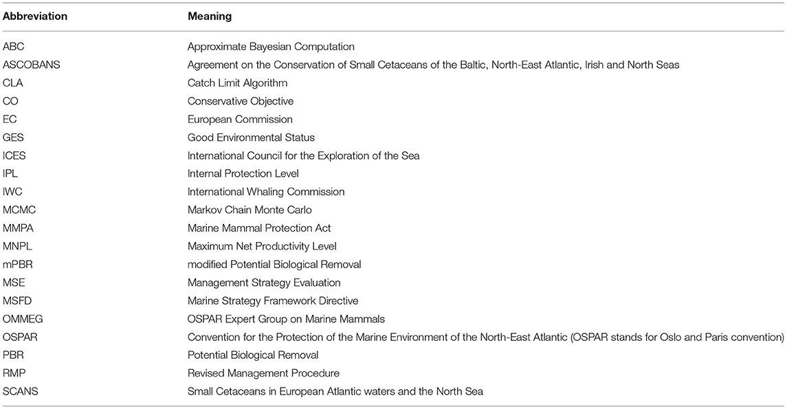
Table 1. Abbreviation used in the paper.
The MMPA has legal teeth because, among others, it spells out a clear quantitative conservation objective (CO) and lays out management objectives and remedial measures to meet the CO. In contrast, a critical gap hindering marine mammal conservation in the European Union (EU) is the lack of (i) a legally-binding CO for marine mammals and (ii) management objectives with respect to human-caused mortality (ICES, 2020b; Rogan et al., 2021). In 2010, the International Council for the Exploration of the Sea (ICES) asked the European Commission (EC) for explicit conservation and management objectives for marine mammal populations (ICES, 2010) but this was not acted upon (see ICES, 2013, pages 35–37 for further discussion). Lacking an explicit CO, the simplest, but also the crudest, approach for assessing the impact of anthropogenic removals on marine mammal populations is to consider a fixed percentage of total abundance as a threshold. For instance, the Agreement on the Conservation of Small Cetaceans of the Baltic, North East Atlantic, Irish and North Seas (ASCOBANS1) passed two resolutions, one in 2000 (Resolution 3.3 on Incidental Take of Small Cetaceans) and the other in 2006 (Resolution 5.5 on Incidental Take of Small Cetaceans) which
• defines “unacceptable interactions” as being, in the short term, a total anthropogenic removal above 1.7% of the best available estimate of abundance (Res.3.3); and
• underlines the intermediate precautionary objective to reduce by-catches to less than 1% of the best available population estimate (Res.3.3 and Res.5.5).
These resolutions make use of a fixed percentage approach to set removal limits due to anthropogenic activities. The EC accepted the ICES (2010) advice to use such an approach (Anonymous, 2010), although without endorsing any of the technical elements within the advice as policy. The fixed percentage approach has been used for small cetaceans, based on the best available recent estimates of abundance and bycatch levels (ICES, 2020b). Several European member states used this approach in their assessment of “Good Environmental Status” (GES) as required by the Marine Strategy Framework Directive (Anonymous, 2008), the overarching instrument to ensure the sustainable use of marine ecosystems in the EU (Korpinen et al., 2021). The advantage of using a fixed percentage of abundance to manage removals lies in its simplicity: only a single estimate of removals and a single estimate of abundance are required. The calculations are transparent, simple, and can be easily followed by all stakeholders. A major shortcoming, however, is how this approach (i) fails to incorporate other information about the population (e.g., life-history parameters) and (ii) does not account for potential errors or bias in estimates or for epistemic uncertainty (i.e., uncertainty about population dynamics; Winship, 2009). Another shortcoming is how, in practice, there is often a temporal mismatch between the available removals and abundance estimates. A conservative approach is to set a removals limit as the management objective which represents an upper bound not to be exceeded. This is the approach followed by the US MMPA and the PBR management strategy (Wade, 1998).
A management strategy is an agreed-upon set of rules for determining thresholds beyond which a CO runs the risk of not being met with unacceptably high probability (Punt, 2006; Winship, 2009; Bunnefeld et al., 2011; Kaplan et al., 2021). This strategy defines management objectives in the form of thresholds that managers can monitor from available data, with the management objectives that these thresholds are not exceeded. As epitomized by the example of whaling, an important scientific insight in the development of precautionary management was the realization that the process of evaluating a management strategy (Management Strategy Evaluation, MSE) was possible with modeling and simulations (Cooke, 1994; Hilborn and Mangel, 1997). MSE thus needs generative models, that is models that can generate (synthetic) data that are similar to observed, and crucially, currently available data. These models need to be more than simple curve-fitting devices and should be infused with ecological realism as much as possible to sustain their long-term use for management. These models are data-generating mechanisms: they can reproduce and simulate the dynamics of an ecological system such as a population subjected to anthropogenic removals on top of natural processes such as density dependence. With these models, scientists can evaluate the performance of management actions in “what-if,” or counterfactual, scenarios to set efficient management objectives. Important, the latter will be gauged against observable and available data (e.g., abundance and bycatch estimates, along with their uncertainties) only and not from unknown quantities (e.g., true abundance; Cooke, 1994). Uncertainties in the underlying model, potential biases and uncertainty in the observed data must be considered in order to ensure that a management strategy is robust to those. Uncertainty should thus be incorporated into management procedures (Punt, 2006) and neither be dismissed as noise nor used to postpone corrective measures by strategic use of ignorance (Mangel et al., 1996; Punt, 2006; Rayner, 2012). Uncertainties and potential biases justify also conservatism in thresholds and rules to avoid running the risk of missing the CO (Mangel et al., 1996).
A management strategy should cover all aspects of management in accordance with pre-specified objectives, including data and analysis requirements, a mathematical formula for calculating thresholds, and a set of rules for all expected situations. Thresholds in the context of marine mammal conservation will take the form of a removals limit, that is an annual maximum number of animals whose removal would not result in excessive depletion of the population. MSE thus requires several components, including:
1. one or several unambiguous quantitative CO;
2. a data simulator (or operating model) to emulate the dynamics of the marine mammal population and the effects of anthropogenic activities on this population;
3. a control rule, whose computation accounts for the expected quantity and quality of observable data, to set a removals limit beyond which the impact of human activities runs the risk of failing the aforementioned CO; and
4. performance metrics, necessarily context-dependent and reflecting the trade-off between the potentially multiple CO defined previously.
All the above are necessary to project forward in time the population dynamics (that is, numbers of animals at each time step, according to population models operating within the data simulator). For each management strategy, the selected control rule is applied: performance metrics are monitored and ultimately assessed with respect to the CO. Items (1) and (4) should be agreed upon by all stakeholders or taken from national or international law if available and transferable. Scientists alone should not be expected or forced to set the CO (Mangel et al., 1996), lest they engage (willingly or not) in “stealth advocacy” which may jeopardize the policy process (Pielke, 2007). Items (2) and (3) fit more squarely under the remit of scientists, whose task is to test a large panel of realistic scenarios to buffer the management strategy against uncertainties and potential biases in the available data. MSE is thus computer intensive as it needs tuning via simulations. Tuning means in the MSE context to find, with a large number of simulations, parameter values of the control rule that meet the CO. Running a large number of simulations has become rather mundane because of the power of modern computers. In practice, however, coding an adequate data simulator may present a daunting task. In addition, to minimize duplication of effort by research groups, and to enhance reproducibility, a common tool is desirable. This is precisely our goal in developing the RLA package for statistical software R which has become the lingua franca of statistical computing for a wide community including many scientists and managers.
Recently, tools to easily run MSE for marine mammals have been developed in the context of the US so-called “import rule” (Williams et al., 2016). These new regulations of the MMPA Import Provision require any nation exporting seafood products to the USA to establish a comparability finding for fisheries that have incidental or intentional mortality and serious injury of marine mammals (Wade et al., 2021). A comparability finding is a demonstration of equivalence in marine mammal conservation effectiveness to those governing bycatch in US fisheries. It requires, among other things, the calculation of a bycatch limit under the PBR control rule. Compliance with these new regulations may be challenging, especially for developing nations (Johnson et al., 2016). Fortunately, tools2 to assist in determining PBR for fisheries of nations exporting sea products to the US have been developed (Siple et al., 2021). Implicit in this context is the acceptance of the MMPA CO: “a population will remain at, or recover to, its maximum net productivity level MNPL (typically 50% of the populations carrying capacity), with 95% probability, within a 100-year period” (Wade, 1998). PBR has been extensively tested (Wade, 1998; Punt et al., 2020a) and its robustness is well established. Yet, MSE is entirely dependent on the CO: if the latter change, a new MSE needs to be carried out. This justifies the need for an applied tool to easily re-run simulations when needed, and to possibly consider control rules other than PBR.
We describe below our RLA package which includes a set of functions to carry out MSE using contemporary population dynamics models for marine mammals species (Punt, 2016). Documentation on MSE for managing marine mammal removals is abundant, yet there is a comparatively dearth of applied tools to carry out MSE (but see Brandon et al., 2017). This gap motivated the development of the package. The manuscript format will be unusual in meshing together in the main text equations and R command lines. This choice is motivated to ease the mapping from the principles of MSE to its application for readers not yet familiar with MSE in practice. Our contribution is to illustrate its use via two cases studies on cetaceans, building on the work of Wade (1998) and Winship (2009) among others. The first case study considers a management strategy under the PBR control rule, then called modified PBR (mPBR), and illustrates tuning it to another CO than the US MMPA, namely the ASCOBANS short-term practical sub-objective “to restore and/or maintain stocks/populations to 80% or more of the carrying capacity” (Res.3.3). The second case study focuses on furthering the development of a Removals Limit Algorithm (RLA) to set limits to anthropogenic mortality of harbor porpoises (Phocoena phocoena) in the North Sea (Winship, 2009; Hammond et al., 2019). The RLA is similar in concept to the Catch Limit Algorithm (CLA) of the International Whaling Commission (IWC)'s Revised Management Procedure (RMP3; Boyce, 2000). We first introduce notations, then detail of the data simulators currently implemented in the RLA package before carrying out the tuning of management strategies with respect to the quantitative interpretation of the ASCOBANS CO made by the Oslo and Paris convention (OSPAR) (Convention for the Protection of the Marine Environment of the North-East Atlantic4) expert group on marine mammals (OMMEG). The article closes on possible extensions of the package.
Materials and Methods
Installation
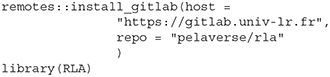
The RLA package for statistical software R (R Core Team, 2020) can be installed from https://gitlab.univ-lr.fr/pelaverse/rla by typing the following in an R (version ≥ 4.0.0) console:
Notation
Notations are detailed in Table 2. Greek letters denote random variables, and the bold font is used to flag a vector of parameters. Let denote the uniform distribution bounded by real numbers l and u. Let denotes the log-normal distribution of location parameter μ and scale parameter σ. The mean of a log-normal random variable y is a function of both the location and scale parameters: . Let Dir(α) denotes the Dirichlet distribution of concentration parameters α. Let Bin(N, π) and Multin(N′, π′) denote, respectively, the binomial distribution of parameters N ∈ ℕ*, π ∈ [0, 1] and multinomial distribution of parameters N′ ∈ ℕ*, ∀π′, π′ ∈ [0, 1] such that ∑π′ = 1.
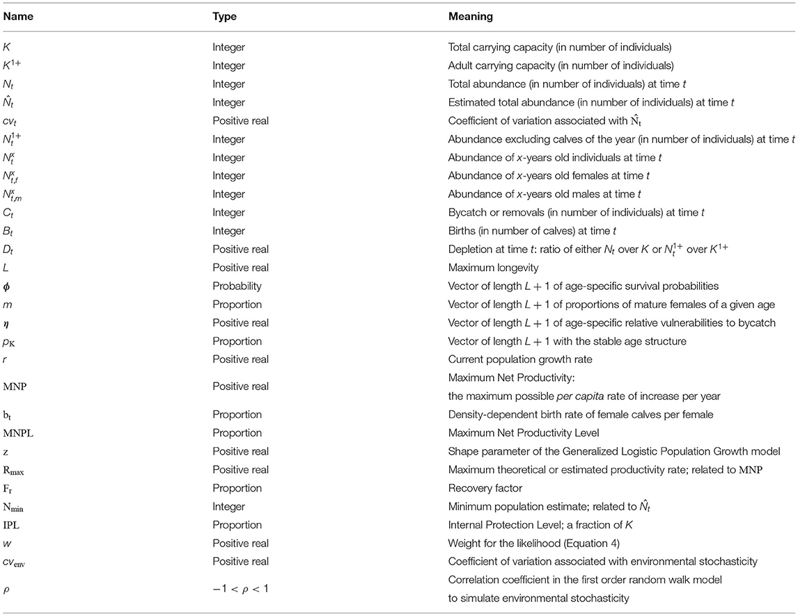
Table 2. Notations.
Potential Biological Removal
Wade (1998) developed a pragmatic approach to set limits to anthropogenic mortality of small cetaceans and pinnipeds with minimal data requirements named PBR. The formula for the removal control rule (the so called “harvest rule” in fisheries science) behind PBR is:
where Rmax is the maximum theoretical or estimated productivity rate of the population (the annual per capita rate of increase in a population resulting from additions due to reproduction, less losses due to natural mortality), Nmin is the minimum population estimate in numbers of animals (i.e., the 20th percentile of the best available abundance estimate, usually the most recent one, assuming a lognormal distribution; Wade, 1998), and Fr is a recovery factor between 0.1 and 1.0.
For small cetaceans, Rmax is difficult to estimate in practice but the value of 4% has been used as a default (Wade, 1998). Fr is most often chosen below 1 (Punt et al., 2018) to (i) account for the current depletion level of the population (the more depleted, the lower) and (ii) allow for some protection against bias and uncertainties in the data: the use of Fr < 1.0 buffers against uncertainties that might prevent population recoveries, such as biases in the estimation of Nmin and Rmax. Wade (1998) determined in a MSE designed for the US MMPA the default value Fr = 0.5 for populations that are depleted, threatened, or of unknown status. The Fr value can be increased up to 1.0 when populations are well studied and biases in the estimation of Nmin and other parameters are thought to be negligible (Punt et al., 2020a). The different values used in Equation (1) were determined by tuning the PBR control rule to the MMPA CO: “a population will remain at, or recover to, its maximum net productivity level MNPL (typically 50% of the population's carrying capacity), with 95% probability, within a 100-year period.” With a different CO, new default values should be determined using MSE (that is, simulations).
The operating model (data simulator) for carrying out simulations with the PBR control rule is a deterministic, age-aggregated, generalized logistic (Pella-Tomlinson) model of population dynamics (refer to Table 2 for notation; Punt, 2016), implemented in the function pellatomlinson_pbr(). A call to the function requires several user-specified inputs, such as the MNPL, to set the appropriate value of parameter z controlling density-dependence. The MNPL corresponds to the level of population depletion at which the population reaches its Maximum Net Productivity (MNP), the maximum renewal rate of the population. The user only needs to specify MNPL: parameter z in Algorithm 1 can be derived with a call to function inverse_MNPL(). Alternatively, the users can directly specify z: for example, z = 2.40 is often used for cetaceans to set MNPL at 0.6K (Wade, 1998).

Algorithm 1. Pella-Tomlinson age-aggregated population dynamics model.
The operating model (Algorithm 1) for carrying out simulations with the PBR control rule assumes that the coefficient of variation of the abundance estimates is sampled from a uniform distribution with a user-defined upper bound, but a lower bound of 10%. This is an assumption about realistic levels of precision that may be achieved on empirical estimates of marine mammal abundance. For example, all estimates from the SCANS-III surveys of marine mammals in the Northeast Atlantic had coefficients of variation larger than 10% (Hammond et al., 2021).
The following code snippet launches a population dynamics simulation, starting at a depletion level of D0 = 5% of K. The population is allowed to grow for 150 years to reach K before removals start and impact the population for 50 years. Removals are generated by randomly drawing a number of caught animals from a uniform distribution (and rounding down to the nearest integer). These removals will deplete the population and can be later used to estimate a removals limit if it can be assumed that these initial removals, which are taking place before implementation of a control rule, can be estimated and are available.
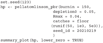
A call to summary_plot() generates Figure 1 to display the population dynamics: the gray area shows the period in which removals are taking place and may deplete the population.
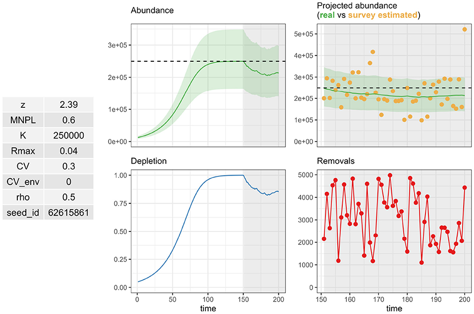
Figure 1. Output from a call to summary_plot() on a pellatomlinson_pbr() output. Inputs are summarized on the left. Population dynamics are displayed in the middle, with either abundance (top) or depletion (bottom). Simulated survey estimates (top) and removals are displayed on the right subfigures.
The function forward_pbr() allows PBR to be tuned to a CO. The function requires the output from pellatomlinson_pbr() and will carry forward the population dynamics using Equation 1 and Algorithm 1 to set limits to anthropogenic removals Ct:
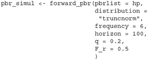
The user needs to specify a time/management horizon, a frequency at which surveys are carried out to estimate population abundance, and a distribution to generate the removals (e.g., a truncated normal distribution; Punt et al., 2021). If unspecified, Rmax is recycled from the previous call to pellatomlinson_pbr(). Other arguments, detailed in the documentation available with ?pellatomlinson_pbr, can be specified to perform “robustness” trials.
To illustrate the capabilities of the implemented functions, a modifed PBR (mPBR) was tuned to the CO “a population should be able to recover to or be maintained at 80% of carrying capacity, with probability 0.8, within a 100-year period.” This CO is a quantitative interpretation from the OMMEG of the ASCOBANS interim objective “to restore and/or maintain stocks/populations to 80% or more of the carrying capacity” (ASCOBANS, 2000). The same MSE as Wade (1998) was carried out (with K = 10, 000), except that the frequency at which survey estimates were assumed to be collected was set to 6 years to match the MSFD reporting cycle. The computation of Nmin was computed as the 20% of a log-normal distribution of mean and associated coefficient of variation cv, which can be computed with the function PBR(). Note that this function relies on directly using quantiles of a log-normal distribution and is slightly different from the calculations presented in Wade (1998) which use quantiles from a normal distribution and exponentiation. Tuning was achieved by evaluating the same base case scenario and “robustness” trials of Wade (1998) with respect to parameter Fr. A base case scenario is a reference situation whereby uncertainties are minimal (e.g., life history or population parameters, such as Rmax or depletion, are known with confidence) and the data are assumed without bias (e.g., no systematic error in abundance estimates). On the other hand, robustness trials address deviations from this base case scenario: “the performance of calculating the PBR in various ways was evaluated under simulations involving plausible flaws in the data or assumptions, such as substantial biases in the abundance or mortality estimates” (Wade, 1998; page 7). For each scenario/trial, 1, 000 simulations were run (Williams et al., 2008), and the final depletion level of the population was monitored after 100 years of using equation (1) to set limits to anthropogenic removals. All simulations were carried out on a Dell laptop latitude 5400 (Intel(R) Core(TM) i7-8665U CPU @ 1.90GHz, 2112MHz, 4 cores, 8 logical processors, 32Gb RAM).
Removals Limit Algorithm
An RLA is derived from the CLA of the IWC's RMP. The RLA is comprised of a statistical model which is fitted to a time series of estimates of abundance and bycatch to estimate population growth rate r and current depletion DT (with T corresponding to the last survey estimate of abundance), both of which are then used in the calculation of a control rule (removals limit). The removals control rule under the RLA, as a fraction of the latest abundance estimate, is given by Equation 2:
where the Internal Protection Level (IPL) is the depletion threshold below which the limit is set to 0. A removals limit of zero is thus used if the estimated current population depletion is less than the IPL, and a non-nil limit, based on estimated stock productivity, is used otherwise (Boyce, 2000). An important difference in the control rule between RLA and PBR is that RLA requires both a time series of abundance estimates and anthropogenic removals (e.g., bycatch). These data are used to estimate the current depletion DT and population growth rate r in the following model (Boyce, 2000):
Particularly, the quantities Nt are not parameters in Equation (3), but quantities that have a deterministic relationship with the unknown parameters r and DT. The latter corresponds to the current population depletion level at the time T of the most recent survey estimate: NT = K × DT gives the final condition for the abundance process in Equation (3) (and thus the model can derive the abundances backward until t = 0). The initial condition is D0 = 1 (that is N0 = K): the population is assumed to be at carrying capacity for t ≤ 0, that is before the start of the time series of estimated anthropogenic removals Ct.
The likelihood ℓ(Nt|r, DT) of a datum Nt under the model specified in Equation (3) is a weighted (with weight w) log-normal probability density function (Boyce, 2000; Aldrin et al., 2008):
The IWC's CLA down-weights the likelihood during model fitting, which represents a departure from the Bayesian paradigm. This down-weighting of the likelihood was found to stabilize the variance in removals limit and improve the performance of the CLA (Cooke, 1999). The rationale for down-weighting information from new data is to limit the speed at which the management procedure responds to feedback. In the RLA, down-weighting of the likelihood is also possible, and is set to w = 1/16 by default (as in the CLA). The likelihood can only be evaluated for the years t* in which survey estimates are available. For those years, and . The full likelihood is .
Estimation of the parameters of model (Equation 3) is carried out in a Bayesian framework, and was coded in Stan (Carpenter et al., 2017). Stan uses Hamiltonian dynamics in Markov chain Monte Carlo (MCMC) to sample values from the joint posterior distribution of DT and r (Carpenter et al., 2017). From this sample, the posterior distribution of Equation (2) is easily obtained and a decision analysis is carried out on which quantile to use to summarize this posterior. With the RLA, tuning is done by selecting a quantile to summarize the posterior distribution of Equation (2). Ultimately, this quantile corresponds to a number of animals, but selecting a quantile allows a dispassionate assessment as the user need not work directly on a number of animals: the number will only be revealed at a later stage.
The model code in Stan syntax is stored as text data in a dataframe within the RLA package and can be accessed with:
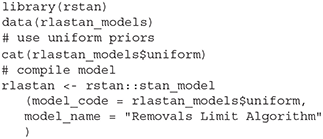
The rstan library (Stan Development Team, 2020) is required for the RLA but is not included among the dependencies of the RLA package so that the user must load the library themself. The model code currently uses uniform priors on both parameters (r, DT). The prior for DT is bounded between 0 and 1, and the prior for r is bounded below by 0 but requires the user to set the upper bound according to the species/population under study. This can be set using the function standata(), which also needs user input on values for IPL and w. The IWC uses IPL = 0.54 and , and these are the default values of the function. This function standata() is primarily meant for MSE with simulations as it requires the output of a call to the function pellatomlinson_rla() which implements a stochastic and age-disaggregated version of a generalized logistic (Pella-Tomlison) model of population dynamics (Algorithm 2). The operating model presented in Algorithm 2 assumes a balanced sex-ratio at birth, and the density-dependent birth rate is expressed as female calves per female by default (hence the factor 2 when simulating the number of calves). The output of pellatomlinson_rla() can be visualized with a call to summary_plot() to generate Figure 2. More specifically, the operating population dynamics model is conditioned on the species/population under study and requires knowledge of age-specific vital rates such as survival and fecundity.

Algorithm 2. Pella-Tomlinson age-disaggregated population dynamics model.
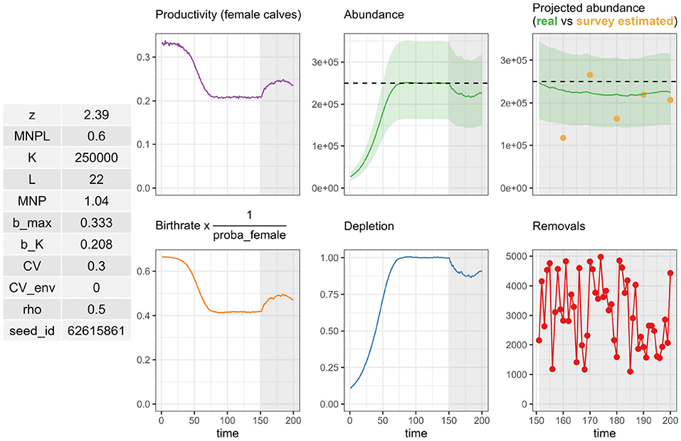
Figure 2. Output from a call to summary_plot() on a pellatomlinson_rla output. Inputs are summarized on the left. Population dynamics are displayed in the middle, with either productivity and abundance (top) or birthrate and depletion (bottom). Simulated survey estimates (top) and removals are displayed on the right sub-figures.
In contrast to the previous example with the PBR control rule, which uses a rather generic (and deterministic) operating model for marine mammal population dynamics, the RLA control rule is used with an operating model conditioned on specific values for a population of a given species. The harbor porpoise in the North Sea is one of the most studied species of marine mammal in European waters. It is also protected in both national and union-level legislation such as the Habitats Directive. In particular, it is listed on both Annexes II and IV of the said directive which requires designation of protected area and strict protection for this species. In the OSPAR Intermediate Assessment 2017, an assessment of harbor porpoise bycatch could not be carried out due to the lack of an agreed upon removals limit and ongoing discussions on methods to set such a limit. In 2009, ICES (2009) advised the European Commission “that a CLA approach is the most appropriate method to set limits on the bycatch of harbor porpoises […].” The use of the RLA control rule for setting removals limit to this species in the North Sea was agreed at OSPAR's biodiversity and ecosystems committee in 2021. For illustration, an RLA was tuned to the CO “the harbor porpoise population in the North Sea should be able to recover to or be maintained at 80% of carrying capacity, with probability 0.8, within a 100-year period.”
Life-history parameters for the harbor porpoise (Phocoena phocoena) in the North Sea were taken from Hammond et al. (2019): they are available as data in the RLA package with data(“north_sea_hp”). The frequency with which survey estimates were assumed to be collected was set to 6 years to match the MSFD reporting cycle. Carrying capacity during the simulations was set to K = 500, 000. The IPL was set to 0.54, that is in a population estimated to be depleted to less than 54% of carrying capacity, the removals limit was automatically set to 0. The weight w was set to . The upper bound for the uniform prior on parameter r was set to 0.1 given recent evidence on the maximum growth rate of harbor porpoise populations (Forney et al., 2021). Tuning was achieved by evaluating the same base case scenario as Hammond et al. (2019) and some “robustness” trials. For each scenario/trial, 1, 200 simulations were run, and the final depletion level of the population was monitored after 100 years of using equation (2) to set limits to anthropogenic removals. The 20th–80th quantile, by an increment of 10, were evaluated. The initial depletion was set between 0.3 and 0.9 of K, with 200 simulations in each bin [0.3:0.4[, …, [0.8:0.9[. The MNPL was drawn from a normal distribution centered on 0.6, with an SD of 0.05 (Figure 3). For the base case scenario, changing the time horizon to 50 or 200 years with respect to the CO was also considered as part of a sensitivity analysis. All simulations were carried out on the supercomputer facilities of the “Mésocentre de calcul de Poitou Charentes (Université de Poitiers/ISAE-ENSMA/La Rochelle Université).”

Figure 3. Inputs for simulations with the Removals Limit Algorithm (RLA). A uniform distribution is induced on the initial depletion level and a normal distribution centered on 0.6 for the Maximum Net Productivity Level (MNPL).
Results
Modified PBR
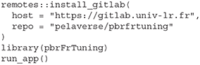
All results can be accessed via a shiny application (Chang et al., 2021), available at https://gitlab.univ-lr.fr/pelaverse/pbrfrtuning:
Base Case Scenario
The CO was reached in the base case scenario with Fr = 0.35 and Fr = 0.60 assuming CV = 0.2 and 0.8, respectively (Figure 4). In other words, with the CO “a cetacean population should be able to recover to or be maintained at 80% of carrying capacity, with probability 0.8, within a 100-year period,” the recovery factor Fr should not be set above 0.6 when abundance is imprecisely estimated, and not above 0.35 when it is precisely estimated. The recovery factor Fr could take a higher value when abundance was imprecisely estimated (larger cv) because Nmin is defined as the 20% quantile of a log-normal distribution. In computing this quantile, the scale and location parameters for the log-normal distribution are, respectively and . A larger cv results both in a larger value for the scale σ and in a lower value for location μ for the same estimated abundance : Nmin is lowered as a result (and the skewness of the distribution, which is solely a function of σ, is increased). This behavior may be visualized with the PBR() function implemented in the package which returns a plot of the assumed log-normal distribution.
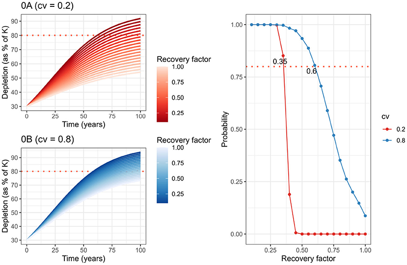
Figure 4. Representation of recovery factor (Fr) impact on depletion level over time for the base case scenario (left) and probability of reaching Conservative Objective (CO) depending on the Fr values (right).
Robustness Trials
Tuning of the recovery factor Fr for the modified PBR is summarized in Table 3. Fr could vary from 0.15 to 1.0 across the different trials. In particular, scenarios in which bycatch was underestimated by a factor 2 or abundance was overestimated by a factor 2 led to selecting a value of Fr = 0.15. Scenarios 7A and 7B, corresponding to a lower MNPL than the one assumed, revealed a lack of robustness as no value of Fr ≥ 0.1 allowed the CO to be reached.
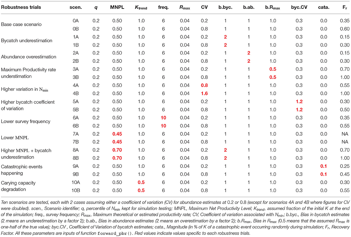
Table 3. Summary of parameters combination for each robustness trial tested and Fr associated.
Differences Between PBR and mPBR for Cetacean Species
Table 3 recapitulates possible choices for Fr depending on several biases or uncertainty. The 8 first scenarios are the same as those of Wade (1998) who found that the value of Fr = 0.50 was sufficient for cetaceans to meet the MMPA CO of reaching at least 50% of carrying capacity with a probability of 0.95 over 100 years. In contrast, with the CO of reaching at least 80% of carrying capacity with probability of 0.8 over 100 years, the sufficient value was Fr = 0.15. This illustrates the change induced by changing the CO between PBR and mPBR for cetacean species.
Removals Limit Algorithm
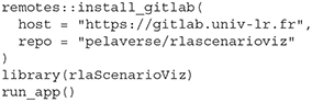
All results can be accessed via a shiny application (Chang et al., 2021), available at https://gitlab.univ-lr.fr/pelaverse/rlascenarioviz:
Base Case Scenario
The CO “the harbor porpoise population in the North Sea should be able to recover to or be maintained at 80% of carrying capacity, with probability 0.8, within a 100-year period” was reached in the base case scenario by selecting the 55th quantile of the control rule given by Equation (2) (Figure 5). This quantile choice corresponded to an average (across all simulations) removals limit set to 1.3% of the best available abundance estimate, or some 5, 600 animals per year (assuming K = 500, 000 animals in the simulations). No change in quantile selection was observed when the time horizon for the CO was lowered to 50 years; but for 200 years, the selected quantile was the 50th, resulting in a somewhat lower removals limit (see shiny application).
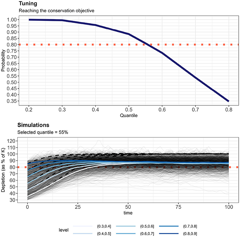
Figure 5. Top panel: Probability to reach the conservation objective (CO) for setting the removals limit as a quantile of the posterior distribution of Equation (2). The 55th quantile is the largest one that allows reaching the CO with a probability of 0.8 after 100 years. Lower panel: All 1, 200 simulations (thick lines: average stratified by initial depletion level) after the implementation of the RLA and removals limit set by using the 55th quantile. The red dotted line shows the 80% of carrying capacity (K). The black hashed line shows average population trajectory if anthropogenic removals were eliminated.
Robustness Trials
Tuning of the RLA is summarized in Table 4. The selected quantile could vary from the 30th to the 80th across the different trials. Trials C and D, corresponding to scenarios in which removals are underestimated by a factor 2, or abundance is overestimated and removals are underestimated both by a factor 1.5, were the most challenging ones to reach the CO. The 30th percentile choice corresponded to an average (across all simulations) removals limit set to 0.5% of the best available abundance estimate, or some 2, 500 animals per year (assuming K = 500, 000 animals in the simulations). These results were obtained by averaging over the uncertainty in both the MNPL (on average occurring at 60% of K) and the initial depletion level (with an average of 60% of K, that is the population being at the MNPL when the RLA is implemented; Figure 3).
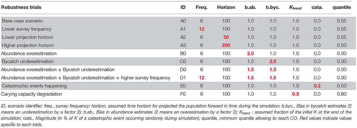
Table 4. Summary of parameter combination for each robustness trial tested and the resulting quantile.
Discussion
Approaches for setting threshold values for removals of protected cetacean species in the Northeast Atlantic have been extensively discussed (see ICES 2019, page 83), with a focus on three approaches in particular: fixed percentages of abundance, PBR, and the CLA developed by the IWC. Of these, the first is both the simplest and the crudest. Its simplicity translated as a direct, off-the-shelf, availability that permitted its use in ASCOBANS resolutions. Yet, its crudity also resulted in the push-back against the approach from scientists and stakeholders alike (for probably different reasons though). In 2009, ICES advised the European Commission that “a Catch Limit Algorithm approach is the most appropriate method to set limits on the bycatch of harbor porpoises or common dolphins” (ICES, 2013). A practical hurdle to using either the PBR or RLA control rule was the lack of tools to carry out a MSE tailored to the European context where the ASCOBANS interim conservation objective is “to restore and/or maintain stocks/populations to 80% or more of the carrying capacity.” We addressed this gap by building an R package to provide scientists with the means of carrying out MSE for setting thresholds on anthropogenic removals of marine mammals. A clear motivation was to remedy the situation seen in the OSPAR Intermediate Assessment 2017 where the recommended approach to setting removals limit could not be implemented.
The RLA package for software R implements utilities to perform the MSE of anthropogenic removals on marine mammal populations (Figure 6). The core functions are two data simulators, pellatomlinson_pbr() and pellatomlinson_rla(), coupled with functions implementing specific control rules: forward_pbr() and forward_rla() for projecting the population forward in time. Around these core functions gravitates a suite of additional functions (Figure 6). The population dynamics simulators are generalized logistic (Pella-Tomlinson) density-dependent models (Punt, 2016) (although other functional forms could be coded and added to the package). Age-aggregated or age-disaggregated versions of the generalized logistic operating model (data simulator) are available. We illustrated the use of these simulators in tuning a modified PBR for small cetaceans (Figure 4 and Table 3) and an RLA for harbor porpoises in the North Sea (Figure 5 and Table 4). In the former case, the simulator is very simple (Algorithm 1) and only allows a very coarse conditioning on species- or population-specific information (e.g., Rmax or Fr; Wade 1998). The age-disaggregated simulator is more involved (Algorithm 2) and allows conditioning on species- or population-specific survival and fecundity when these are known. It is also possible to use the age-disaggregated simulator pellatomlinson_rla() with the PBR control rule with function pbr_nouveau() as in e.g. Brandon et al. (2017) or Punt et al. (2020a). This allows conditioning on species- or population-specific survival and fecundity data in the population dynamics model for increased realism, but relying on minimal data (abundance estimates only) to design a precautionary MSE. Both simulators as currently implemented assume a single population of a single species, which can be limiting. Extension to multiple populations of the same species, or multiple species (Punt et al., 2020b; Kanaji et al., 2021; Kaplan et al., 2021) are potential extensions of the operating models within the simulators. In particular, consideration of migration between populations would account for potential sink-source dynamics. This could lead to a more accurate and realistic MSE. This would also need to potentially consider different removals limits for different populations, either to reflect the sink-source distinction or to account for transboundary differences in management if populations are managed by different parties/states or subjected to several fisheries.
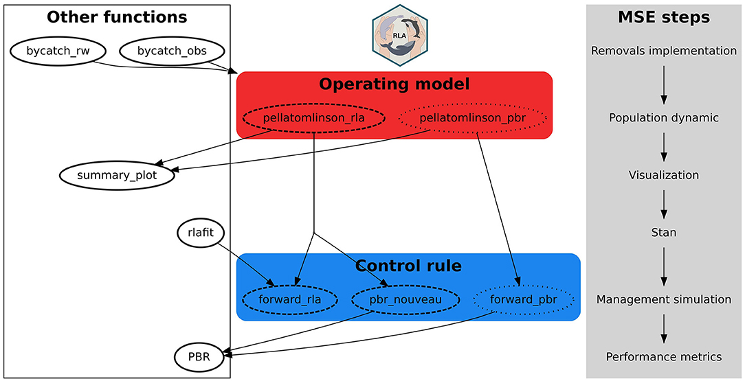
Figure 6. Package structure with the core functions to carry out Management Strategy Evaluation (MSE).
Albeit currently limited to single-population, single-species, and single-control rule, the RLA package provides a convenient implementation of population dynamics simulators, which can be leveraged to design a precautionary management strategy by means of robustness trials (Wade, 1998). These robustness trials include consideration of
• systematic bias in abundance or removal estimates;
• random errors in removal estimates, either before or after the implementation of a control rule;
• random catastrophic mortality events killing off a fraction of the population (e.g., epizootics; Aguilar and Raga, 1993);
• a decline in carrying capacity K over time;
• environmental stochasticity on population dynamics with a correlated, first order, random walk model;
• differential vulnerabilities to the removal with respect to age.
All these trials can currently be run with the RLA package as exemplified by the two case studies presented herein (Tables 3, 4). They use different control rules, either PBR or RLA, reflecting a difference in the data assumed available for management. The output of simulations is, however, the same as the whole population trajectory under the chosen control rule is available to the user. From this output, additional work is required from the user to analyze the strategy with respect to performance metrics.
Performance metrics with respect to the CO are left to user discretion: there are no special functions in the RLA package to compute specific performance metrics. As the output from the core functions include the whole population trajectory, removals, etc. (Figures 1, 2), there is user flexibility for computing performance metrics. In the two case studies, the only performance metric that was assessed was whether the CO was reached after 100 years of implementation of a control rule for computing the removals limit. The probability with which the CO was reached was computed as the frequency of simulations with final depletion ≥ 80% of K over all simulations. One straightforward additional performance metric is the delay in population recovery with the implementation of the removals limit compared to a counterfactual situation whereby anthropogenic removals were eliminated. This metric was computed for the RLA case study (as shown in Results and associated shiny applications) using the function time2CO which requires the user to specify a number of consecutive years for which the CO must have been reached to declare success. This function calls another function get_streaks which will identify streaks of 0 and 1 in a vector. The output of a simulation includes a vector named depletion which can be used to compute the time to reach the CO as follows:

As each simulation output reports an identifier, which is also a seed that the user can set, it is possible to match the result from a removals limit implementation with the counterfactual outcome under no anthropogenic removals (by using the same seed in both cases). This feature allows performance comparisons under counterfactuals as random number generation remains under user control.
One strength of the RLA package is the enhanced flexibility for users. In addition to defining CO and performance metrics, advanced users familiar with Stan syntax can code their own model, or modify the ones stored as text in a list available in the package, to implement different control rules to set a removals limit. The only requirement is to use a parameter or derived quantity from parameters with the name removal_limit for function forward_rla() to work. For example, the removals limit could change (by hard coding in Stan syntax; as shown in Methods above and mc-stan.org) from
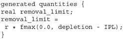
to the IWC CLA (e.g., Aldrin et al. 2008; but note that the IWC CLA5 differs also with respect to Equation 3)
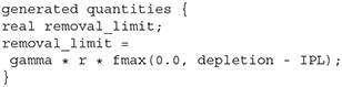
where the scalar gamma must be defined by the user in the transformed data block.
As noted by a reviewer, the currently implemented statistical model for estimating current depletion and population growth rate in the RLA control rule (Equation 3) assumes the population is at carrying capacity before the time series of removals starts. Implicitly, this assumes that data on anthropogenic removals are available from the start of human impacts on marine mammal populations. This assumption is likely wrong in many instances, but convenient, as the available time series of removals may not extend back to pristine conditions. The assumption could be relaxed in using an alternative statistical model with an extra parameter on the initial depletion. The latter is not estimable from the abundance and removal data alone, and an informative prior would be needed to ensure identifiability. Alternatively, an additional robustness trial may be considered: in this trial, the removals data would be left-truncated (that is the start of the series would be unavailable to the investigator) and the performance of the currently implemented model assessed. Depending on the results, an alternative model specification may be needed.
The Stan engine for Bayesian inference using Hamiltonian Monte Carlo (Carpenter et al., 2017) is versatile and allows to fit a large set of models with efficient algorithms (Monnahan et al., 2017). This versatility may be leveraged by advanced users: function forward_rla() needs an object of class “stanmodel” to run. This object is a compiled model that will be repeatedly used within function forward_rla(), thus minimizing model compilation time for a faster run. For example, with a time horizon of 100 years and an assumed frequency of 6 years, function forward_rla() calls internally times the function sampling from package rstan (Stan Development Team, 2020) in a single simulation. While a single simulation with forward_rla() takes a couple of minutes on a laptop, running a large number of simulations quickly becomes prohibitively long. However, computing clusters can be used and resulted in our case of ≈ 36 h to run 1, 200 simulations (and hence 1, 200 × 17 = 20, 400 calls to sampling). Further gains in computation time may be leveraged by taking advantages of parallelization with Stan (interested readers can refer to the Stan manual: https://mc-stan.org/docs/2_27/stan-users-guide/parallelization-chapter.html).
The use of Hamiltonian Monte Carlo for inference on parameters needed for the RLA is justified as sampling from the joint posterior distribution of parameters of equation (3) can be difficult: parameters r and DT are often positively correlated. Further work on priors other than independent uniform distribution may help. We plan to explore the use of a joint prior to model the correlation between r and DT, using for example, a copula (dos Santos Silva and Freitas Lopez, 2008). Further work on the weight w should also be undertaken to assess the sensitivity of RLA to the current choice inherited from the IWC's CLA. The RLA as currently implemented in the package RLA differs from the IWC's CLA: these differences may have consequences that deserve more scrutiny. In particular, we found that increasing the time horizon from 100 to 200 years actually decreased the removals limit, while the reverse was found with the CLA (Aldrin et al., 2008). While surprising and requiring a more in-depth investigation with respect to its cause, this result may currently provide a disincentive to unambitious CO with a long-time horizon to address the issue of unsustainable anthropogenic impacts on marine mammals.
The RLA package is primarily geared toward MSE for setting precautionary limits to anthropogenic removals in marine mammal conservation. The population dynamics simulator provided by Algorithm 2 may however be harnessed for other uses such as Approximate Bayesian Computation (ABC; Beaumont, 2010; Csilléry et al., 2010). In practice, the generalized logistic model may be difficult to fit directly, and one may resort to likelihood-free methods to carry out inferences on a subset of parameters of interest such as survival (ϕ), maturity (m), density-dependence (z), or historic removals (assuming, for example, a simple generative model such as Poisson with constant rate). In this case, summary statistics would be the abundance estimates: a rejection algorithm (as available for example in package abc; Csillery et al., 2012) can be run using the observed abundance estimates and the simulated ones to infer parameters of interest. Not all parameters may be realistically inferred and some may need to be fixed, or highly informative priors may be needed.
Future Applications
We have described the RLA package, which provides a set of functions to carry out the MSE of anthropogenic removals on marine mammals. The two case studies presented were initially carried out under the remit of OMMEG to tune the PBR control rule to the ASCOBANS CO and to continue developing an RLA for harbor porpoise in the North Sea (Hammond et al., 2019). While documentation on MSE was abundant, OMMEG was faced with a dearth of applied tools, which motivated the development of the package. Results obtained and presented need to move through the OSPAR policy process but suggest new default values for the recovery factor Fr with the PBR control rule for small cetaceans and using the 30th quantile with the RLA (Equations 2 and 3) control rule for harbor porpoise to set removals limit in the North Sea. The results for mPBR reported in Table 3 provide first results on values of the recovery factor Fr for setting removals limit to cetacean bycatch in accordance with the OMMEG interpretation of the ASCOBANS CO. A very conservative choice is Fr = 0.1 because of a lack of robustness of mPBR against an MNPL lesser than 0.5. However, such low values of MNPL are implausible for marine mammal populations (Taylor and DeMaster, 1993). More plausible scenarios are those wherein bycatch is underestimated (ICES, 2020a), although assuming an underestimation by a factor 2 maybe be extreme in some cases. Further work on mPBR conditioned on specific contexts within European waters is necessary, especially in considering realistic robustness trials for optimal realism and plausibility.
In the case of the harbor porpoise in the North Sea, the results presented in Table 4 averaged over a large range of initial depletion. Using the 30th quantile is a very conservative default which can be relaxed in practice when more evidence and information on specific species and areas of interest are available (for example, to narrow down the plausible range of initial depletion). The actual removals limit to be used for example in the next OSPAR assessment for the 2023 Quality Status Report (https://www.ospar.org/work-areas/cross-cutting-issues/qsr2023) needs to be calculated on the best available evidence, including the latest SCANS-III survey abundance estimates (Hammond et al., 2021) and bycatch estimates in the North Sea. This illustrates that implementation of management of bycatch based on removal limits derived from PBR and RLA is dependent on the continuation of cetacean population monitoring programs on a scale commensurate with biological meaningful assessment units (see for example North Atlantic Marine Mammal Commission and the Norwegian Institute of Marine Research 2019 page 13 for assessment units of harbor porpoises). A modified PBR tuned to OMMEG's interpretation of the ASCOBANS CO, namely “a population should be able to recover to or be maintained at 80% of carrying capacity, with probability 0.8, within a 100-year period” will address a current misalignment between management and conservation objectives in the salient context of small cetacean conservation in the Northeast Atlantic (ICES, 2020c). It is our hope that the RLA package will enable easier MSE, in particular in the current EU MSFD context of achieving “Good Environmental Status.” This hope crucially hinges on users' feedback and involvement in further developing and expanding the package to the benefit of improved management of the impact of human activities on marine mammals.
Data Availability Statement
All codes and datasets used in this study are available at https://gitlab.univ-lr.fr/pelaverse/rla_paper.
Author Contributions
MG and MA led the analyses, the conception, and writing of the paper and package. All authors supported in analyses, paper conception, writing and contributed to the article and approved the submitted version.
Funding
ADERA provided support in the form of salaries for MA but did not have any additional role in the study design, data collection and analysis, decision to publish, or preparation of the manuscript.
Conflict of Interest
MA is employed by the commercial company ADERA which did not play any role in this study beyond that of employer. AW is employed by the commercial company CSS, Inc. KM is employed by the commercial company HiDef.
The remaining authors declare that the research was conducted in the absence of any commercial or financial relationships that could be construed as a potential conflict of interest.
Publisher's Note
All claims expressed in this article are solely those of the authors and do not necessarily represent those of their affiliated organizations, or those of the publisher, the editors and the reviewers. Any product that may be evaluated in this article, or claim that may be made by its manufacturer, is not guaranteed or endorsed by the publisher.
Acknowledgments
AG thanks the German Federal Agency for Nature Conservation for funding her time as the lead of the OSPAR expert group on marine mammals. MA and MG thank Mikaël Guichard and the dedicated staff at the Mésocentre de Calcul de Poitou Charentes. We thank reviewers, Finn Larsen, Lotte Kindt-Larsen, and OMMEG members for discussion and critical comments.
Footnotes
1. ^https://www.ascobans.org/en/species/threats/bycatch
2. ^https://github.com/mcsiple/mmrefpoints
References
Aguilar, A., and Raga, J. A. (1993). The stripped dolphin epizootic in the Mediterranean sea. Ambio 22, 524–528.
Aldrin, M., Husevy, R. B., and Schweder, T. (2008). A note on tuning the catch limit algorithm for commercial baleen whaling. J. Cetacean Manag. Res. 10, 191–194.
Anonymous (2008). Directive 2008/56/EC of the European Parliament and of the Council of 17 June 2008 establishing a framework for community action in the field of marine environmental policy (Marine Strategy Framework Directive) (Text with EEA relevance). Official Journal of the European Union. 2008/56/EC.
Anonymous (2010). Letter from the european commission to ices, dated 29 july 2010. ref. ares(2010)830555 - 18/11/2010. Letter.
ASCOBANS (2000). Annex O - Report of the IWC-ASCOBANS working group on harbour porpoises. J. Cetacean Res. Manag. 2(Suppl.):297–305.
Authier, M., Galatius, A., Gilles, A., and Spitz, J. (2020). Of power and despair in cetacean conservation: estimation and detection of trend in abundance with noisy and short time-series. PeerJ 8:e9436. doi: 10.7717/peerj.9436
Avila, I. C., Kaschner, K., and Dormann, C. F. (2018). Current global risks to marine mammals: taking stock of the threats. Biol. Conserv. 221, 44–58. doi: 10.1016/j.biocon.2018.02.021
Beaumont, M. (2010). Approximate bayesian computation in evolution and ecology. Ann. Rev. Ecol. Evolut. Syst. 41, 379–406. doi: 10.1146/annurev-ecolsys-102209-144621
Boyce, M. S. (2000). Quantitative Methods for Conservation Biology, Chapter Whaling Models for Cetacean Conservation. New York, NY: Springer, 109–126.
Brandon, J. R., Punt, A. E., Moreno, P., and Reeves, R. R. (2017). Toward a tier system approach for calculating limits on human-caused mortality of marine mammals. ICES J. Mar. Sci. 74, 877–887. doi: 10.1093/icesjms/fsw202
Brownell, R. Jr, Reeves, R., Read, A., Smith, B., Thomas, P., Ralls, K., et al. (2019). Bycatch in gillnet fisheries threatens critically endangered small cetaceans and other aquatic megafauna. Endanger. Species Res. 40, 285–296. doi: 10.3354/esr00994
Bunnefeld, N., Hoshino, E., and Milner-Gulland, E. J. (2011). Management strategy evaluation: a powerful tool for conservation? Trends Ecol. Evol. 26, 441–447. doi: 10.1016/j.tree.2011.05.003
Carpenter, B., Gelman, A., Hoffman, M. D., Lee, D., Goodrich, B., Betancourt, M., et al. (2017). Stan: a probabilistic programming language. J. Stat. Softw. 76, 1–32. doi: 10.18637/jss.v076.i01
Chang, W., Cheng, J., Allaire, J., Sievert, C., Schloerke, B., Xie, Y., et al. (2021). shiny: Web Application Framework for R. R package version 1.6.0.
Cooke, J. G. (1999). Improvement of fishery-management advice through simulation testing of harvest algorithms. ICES J. Mar. Sci. 797–810. doi: 10.1006/jmsc.1999.0552
Csilléry, K., Blum, M., Gaggiotti, O., and François, F. (2010). Approximate bayesian computation (ABC) in practice. Trends Ecol. Evol. 25, 410–418. doi: 10.1016/j.tree.2010.04.001
Csillery, K., Francois, O., and Blum, M. G. B. (2012). abc: an r package for approximate bayesian computation (abc). Methods Ecol. Evolut. 3, 475–479. doi: 10.1111/j.2041-210X.2011.00179.x
dos Santos Silva, R., and Freitas Lopez, H. (2008). Copula, marginal distributions and model selection: a bayesian note. Stat. Comput. 18, 313–320. doi: 10.1007/s11222-008-9058-y
Forney, K. A., Moore, J. E., Barlow, J., Carretta, J. V., and Benson, S. R. (2021). A multidecadal bayesian trend analysis of harbor porpoise (Phocoena phocoena) populations off california relative to past fishery bycatch. Mar. Mamm. Sci. 37, 546–560. doi: 10.1111/mms.12764
Gerrodette, T. (1987). A power analysis for detecting trends. Ecology 68, 1364–1372. doi: 10.2307/1939220
Gray, C. A., and Kennelly, S. J. (2018). Bycatches of endangered, threatened and protected species in marine fisheries. Rev. Fish. Biol. Fish. 28, 521–541. doi: 10.1007/s11160-018-9520-7
Hammond, P. S., Lacey, C., Gilles, A., Viquerat, S., Börjesson, P., Herr, H., et al. (2021). Estimates of Cetacean Abundance in European Atlantic Waters in Summer 2016 from the SCANS-III Aerial and Shipboard Surveys. Technical report, Sea Mammal Research Unit, University of St Andrews, UK.
Hammond, P. S., Paradinas, I., and Smout, S. C. (2019). Development of a Removals Limit Algorithm (RLA) to Set Limits to Anthropogenic Mortality of Small Cetaceans to Meet Specified Conservation Objectives. JNCC Report No. 628. (Peterborough: JNCC). Available online at: https://data.jncc.gov.uk/data/8ac9a424-eda5-4062-957e-63d82d3e39cc/JNCC-Report-628-FINAL-WEB.pdf
Hilborn, R., and Mangel, M. (1997). The Ecological Detective. Confronting Models With Data, 1st Edn. Princeton, NJ: Princeton University Press.
ICES (2009). Report of the Study Group for Bycatch of Protected Species (SGBYC). Technical Report, ICES CM 2009/ACOM:22. 19-22 January 2009, Copenhagen, Denmark, 117.
ICES (Ed.). (2010). General Advice EC Request on Cetacean Bycatch Regulation 812/2004, Item 3. Copenhagen: International Council for the Exploration of the Sea.
ICES (2013). Report from the Working Group on Bycatch of Protected Species, (WGBYC). Technical Report No. ICES CM 2013/ACOM:27, International Council for the Exploration of the Sea, 4–8 February, Copenhaguen, 73.
ICES (Ed.). (2019). Report of the Working Group on Marine Mammal Ecology (WGMME), volume 11–14 February 2019, ICES Scientific Reports. 1:22, Büsum, International Council for the Exploration of the Sea, 131.
ICES (2020a). Report from the Working Group on Bycatch of Protected Species, (WGBYC). Tech report 2:81, International Council for the Exploration of the Sea, 209.
ICES (Ed.). (2020b). Report of the Working Group on Marine Mammal Ecology (WGMME), volume 10-14 February 2020, Barcelona, ICES Scientific Reports. 2:39. International Council for the Exploration of the Sea, 85.
ICES (2020c). Workshop on fisheries Emergency Measures to minimize BYCatch of short-beaked common dolphins in the Bay of Biscay and harbour porpoise in the Baltic Sea (WKEMBYC). Resreport 2:43, International Council for the Exploration of the Sea. 354.
Johnson, A. F., Caillat, M., Verutes, G. M., Peter, C., Junchompoo, C., Long, V., et al. (2016). Poor Fisheries Struggle with U.S. Import Rule Sci. 355, 1031–1032. doi: 10.1126/science.aam9153
Kanaji, Y., Maeda, H., Okamura, H., Punt, A. E., and Branch, T. (2021). Multiple-model stock assessment frameworks for precautionary management and conservation on fishery-targeted coastal dolphin populations off Japan. J. Appl. Ecol. 58, 2479–2492. doi: 10.1111/1365-2664.13982
Kaplan, I. C., Gaichas, S. K., Stawitz, C. C., Lynch, P. D., Marshall, K. N., Deroba, J. J., et al. (2021). Management strategy evaluation: allowing the light on the hill to illuminate more than one species. Front. Mar. Sci. 8:664355. doi: 10.3389/fmars.2021.624355
Korpinen, S., Laamanen, L., Bergström, L., Nurmi, M., Andersen, J. H., Haapaniemi, J., et al. (2021). Combined effects of human pressures on Europe's marine ecosystems. Ambio 50, 1325–1336. doi: 10.1007/s13280-020-01482-x
Mangel, M., Talbot, L. M., Meffe, G. K., Agardy, M. T., Alverson, D. L., Barlow, J., et al. (1996). Principles for the conservation of wild living resources. Ecol. Appl. 6, 338–362. doi: 10.2307/2269369
Monnahan, C. C., Thorson, J. T., and Branch, T. A. (2017). Faster estimation of bayesian models in ecology using hamiltonian monte carlo. Methods Ecol. Evolut. 8, 339–348. doi: 10.1111/2041-210X.12681
North Atlantic Marine Mammal Commission and the Norwegian InstituteNorth Atlantic Marine Mammal Commission and the Norwegian Institute of Marine Research (2019). Report of Joint IMR/NAMMCO International Workshop on the Status of Harbour Porpoises in the North Atlantic. Technical report, Tromsøo.
Pielke, R. A. Jr. (2007). The Honest Broker - Making Sense of Science in Policy and Politics, 1st Edn. Cambridge: Cambridge University Press, 198 ISBN: 9780521873208.
Punt, A. E. (2006). The FAO precautionary approach after almost 10 years: have we progressed towards implementing simulation-tested feedback-control management systems for fisheries management? Natural Resour. Model. 19, 441–464. doi: 10.1111/j.1939-7445.2006.tb00189.x
Punt, A. E. (2016). Review of Contemporary Cetacean Stock Assessment Models. Technical report, School of Aquatic and Fishery Sciences, University of Washington, Seattle, WA.
Punt, A. E., Moreno, P., Brandon, J. R., and Mathews, M. A. (2018). Conserving and recovering vulnerable marine species: a comprehensive evaluation of the US approach for marine mammals. ICES J. Mar. Sci. 75, 1813–1831. doi: 10.1093/icesjms/fsy049
Punt, A. E., Siple, M., Francis, T. B., Hammond, P. S., Heinemann, D., Long, K. J., et al. (2020a). Robustness of potential biological removal to monitoring, environmental, and management uncertainties. ICES J. Mar. Sci. 77, 2491–2507. doi: 10.1093/icesjms/fsaa096
Punt, A. E., Siple, M., Francis, T. B., Hammond, P. S., Heinemann, D., Long, K. J., et al. (2021). Can we manage marine mammal bycatch effectively in low-data environments? J. Appl. Ecol. 58, 596–607. doi: 10.1111/1365-2664.13816
Punt, A. E., Siple, M., Sigurðsson, G. M., Víkingsson, G., Francis, T. B., Granquist, S. M., et al. (2020b). Evaluating management strategies for marine mammal populations: an example for multiple species and multiple fishing sectors in Iceland. Can. J. Fish. Aquatic Sci. 77, 1316–1331. doi: 10.1139/cjfas-2019-0386
R Core Team (2020). R: A Language and Environment for Statistical Computing. Vienna: R Foundation for Statistical Computing.
Rayner, S. (2012). Uncomfortable knowledge: the social construction of ignorance in science and environmental policy discourses. Econ. Soc. 41, 107–125. doi: 10.1080/03085147.2011.637335
Reeves, R. R., McClellan, K., and Werner, T. B. (2013). Marine mammal bycatch in gillnet and other entangling net fisheries, 1990 to 2011. Endanger. Species Res. 20, 71–97. doi: 10.3354/esr00481
Rogan, E., Read, A. J., and Berggren, P. (2021). Empty promises: the european union is failing to protect dolphins and porpoises from fisheries by-catch. Fish Fish. 22, 865–869. doi: 10.1111/faf.12556
Siple, M. C., Punt, A. E., Francis, T. B., Hammond, P. S., Heinemann, D., Long, K. J., et al. (2021). mmrefpoints: Projecting long-term marine mammal abundance with bycatch. R package version 1.0.0.
Taylor, B., Martinez, M., Gerrodette, T., Barlow, J., and Hrovat, Y. (2007). Lessons from monitoring trends in abundance of marine mammals. Mar. Mamm. Sci. 23, 157–175. doi: 10.1111/j.1748-7692.2006.00092.x
Taylor, B. L., and DeMaster, D. P. (1993). Implications of non-linear density dependence. Mar. Mamm. Sci. 9, 360–371. doi: 10.1111/j.1748-7692.1993.tb00469.x
Wade, P. R. (1998). Calculating limits to the total allowable human-caused mortality of cetaceans and pinnipeds. Mar. Mamm. Sci. 14, 1–37. doi: 10.1111/j.1748-7692.1998.tb00688.x
Wade, P. R., Long, K. J., Francis, T. B., Punt, A. E., Hammond, P. S., Heinemann, D., et al. (2021). Best practices for assessing and managing bycatch of marine mammals. Front. Mar. Sci. 8:1566. doi: 10.3389/fmars.2021.757330
Williams, R., Burgess, M. G., Ashe, E., Galnes, S. D., and Reeves, R. (2016). U.S. Seafood import restriction presents opportunity and risk. Science 354, 1372–1374. doi: 10.1126/science.aai8222
Williams, R., Hall, A., and Winship, A. (2008). Potential limits to anthropogenic mortality of small cetaceans in coastal waters of British Columbia. Can. J. Fish. Aquatic Sci. 65, 1867–1878. doi: 10.1139/F08-098
Keywords: bycatch, conservation, management, marine mammal, PBR, RLA, R
Citation: Genu M, Gilles A, Hammond PS, Macleod K, Paillé J, Paradinas I, Smout S, Winship AJ and Authier M (2021) Evaluating Strategies for Managing Anthropogenic Mortality on Marine Mammals: An R Implementation With the Package RLA. Front. Mar. Sci. 8:795953. doi: 10.3389/fmars.2021.795953
Received: 15 October 2021; Accepted: 24 November 2021;
Published: 24 December 2021.
Edited by:
Lars Bejder, University of Hawaii at Manoa, United StatesReviewed by:
Debra Palka, Northeast Fisheries Science Center (NOAA), United StatesClaudio Vasapollo, Istituto Superiore per la Protezione é la Ricerca Ambientale (ISPRA), Italy
Copyright © 2021 Genu, Gilles, Hammond, Macleod, Paillé, Paradinas, Smout, Winship and Authier. This is an open-access article distributed under the terms of the Creative Commons Attribution License (CC BY). The use, distribution or reproduction in other forums is permitted, provided the original author(s) and the copyright owner(s) are credited and that the original publication in this journal is cited, in accordance with accepted academic practice. No use, distribution or reproduction is permitted which does not comply with these terms.
*Correspondence: Matthieu Authier, bWF0dGhpZXUuYXV0aGllckB1bml2LWxyLmZy