 Miao Fan
 Suixiang Shi2
 Yong Ma
 Hu Wang
 Xuefeng Zhang
 Pengfei Ning
- 1School of Marine Science and Technology, Tianjin University, Tianjin, China
- 2Marine Surveying and Geospatial Department, National Marine Data and Information Service, Tianjin, China
The benthic structure of seamounts is critical for understanding the ecological environment and for assessing the influence of resource exploitation. However, the characteristics of the benthic structure of the seamount, especially for guyot, are still far from being clearly understood. For the first time, we carried out detailed hydroacoustic mapping in conjunction with surficial sediment sampling and underwater video recording to investigate the geomorphical and biological characteristics of Pallada Guyot in the Western Pacific Ocean (WPO). We utilized the Benthic Terrain Modeler (BTM) as an initial step to describe the detailed benthic structures and then classify the textural seabed according to backscatter images and sediment samples. We further discussed the relationship between geomorphology and the occurrence of benthic megafauna from video images. The results revealed that 13 classes of benthic structural zones were differentiated, and the dominant zones were flat abyssal plains, where the number and size of megafauna were smaller than those on the flank and flat-topped areas. The second most notable feature is the flat top, where sea cucumbers, starfish, fish, and shrimp have higher biomass and diversity. In the flank region, which is characterized by complex and extensive current-scoured ridges and depressions, sponges and corals are distributed in high-relief bedrocks. We also found that the maximum water depth where cold-water corals develop is 2,250 m. The sponge grounds appear in a marked bathymetric belt (1,800–2,150 m), which is shallower than that on a tropical seamount (2,500–3,000 m) located in the northeastern Atlantic. The findings of this study contribute to understanding the geomorphological drivers and biogeography of WPO seamounts and provide a reference for identifying priority areas for improved marine mineral planning in WPO areas.
Introduction
Benthic habitats are spatial representations of physically distinct areas of the seafloor that are associated with particular groups of plants and animals (Ismail et al., 2015; Harris and Baker, 2020). Geomorphological studies help to comprehend the complexity of seafloor patterns, which can condition a number of environmental characteristics, such as light incidence, hydrologic and energy cycling, nutrient availability, and substrate, which act as proxies for the occurrence and abundance of benthic biota (Harris et al., 2014; Vincent et al., 2016; Goes et al., 2019). Because of the difficulties and expenses of biological sampling in the deep sea, efficient geomorphological mapping based on bathymetry or backscatter intensity is widely used as the basis for benthic habitat mapping to learn about physical habitats (McArthur et al., 2010; Craig et al., 2011; Coiras et al., 2011; Serrano et al., 2017).
Seamounts are features with an elevation greater than 1,000 m above the deepest isobaths of the surrounding seabed (IHO, 2019) and are believed to be hotspots for many endemic species, including large pelagic angles, sharks, pinnipeds, cetaceans, and seabirds (Hubbs, 1959; Richer de Forges et al., 2000; Clark et al., 2010; Rogers, 2018). However, the biodiversity and ecosystems of seamounts face a number of threats, including overfishing, marine litter, and potentially deep-sea mining. Mineral deposits, such as cobalt crusts, seabed sulfides, and marine phosphates, usually develop in association with seamounts. Deep-sea mining is becoming increasingly attractive due to the above-mentioned metal-rich deep-sea minerals (Hein et al., 2013), for example, Japan conducted the world’s first excavation of cobalt-rich seabed in the deep ocean in 2020 (JOGMEC, 2020). The regions with the highest financial potential are believed to be in the tropical West Pacific—for instance, the Magellan Seamounts have been authorized for mineral exploration (Halbach et al., 2017; ISA, 2018; Yang et al., 2020).
Considerable investigation of the marine biogeography of seamounts has concluded that many environmental factors, including depth, topography, substrate, water mass properties (temperature, salinity, and oxygen content), current speed, and primary production, can influence both the composition and distribution of benthic assemblages of seamounts (Wienberg et al., 2013; Serrano et al., 2017; Morgan et al., 2019; Jun Ma et al., 2021a; Jun Ma et al., 2021b). Depth, slope, biogeographic region, topography, and substrate type are common geomorphological factors. However, the geomorphological factors that best explain the changes in species or community structures still require further discussion. Davies et al. (2015) believed that depth and substrate type are key factors in determining the distribution of soft-bottom biomes, while cold-water corals are mainly distributed on the radiating ridges on both sides of the seamount shallower than 1,500 m in the Anton Dohrn Seamount in the Northeast Atlantic. Goode et al. (2021) studied the structure and distribution of giant benthic communities on two seamounts in different physical environments in New Zealand and arrived at different conclusions that the community on one seamount is belt-distributed with increasing depth, while the community on the other is mainly distributed with slope aspect and pinnacle topography. Du Preez et al. (2016) believed that depth and roughness are the most important factors for predicting the structure of giant seafloor biomes in the Cobb Seamount in the northeast Pacific. Bridges et al. (2021) argued that depth is the most important factor affecting the biomes of the 13 South Atlantic Seamount. Therefore, the environmental variables that best explain the variations in community structure differ between seamounts at different spatial scales.
The guyot, a type of flat-topped seamount that has a different geological background compared with a common seamount, is believed to have breached the sea surface, waves, and other subaerial processes such as wind, rainfall, and weathering that eroded the flanks. Guyots are particularly developed in the Western Pacific Ocean (WPO) rather than in other oceans. Despite several applications of geophysical analysis to infer mineral distributions (Ma et al., 2013; Yang et al., 2020), to our knowledge, no benthic habitat study from a geophysical perspective has been undertaken to date to create reliable benthic structure maps. The unprecedented detail and the complete coverage of the multibeam sonar dataset have enabled new insights into the guyot geomorphology. Therefore, describing detailed benthic structures is a valuable means to highlight species–environment relationships as well as to identify habitats to protect (Lecours et al., 2016).
In this study, the benthic structure of a typical deep-sea guyot in the WPO was investigated through the Benthic Terrain Modeler (BTM) and backscatter classification based on two decades of systematic investigation. Furthermore, geomorphological controls on the occurrence of benthic megafauna are discussed. Our objectives were to (1) identify unprecedented benthic structures from the geomorphological view of typical WPO guyots, (2) determine which geomorphological factors control the distribution of benthic megafauna, and (3) summarize the patterns of the benthic structure of typical WPO guyots and provide a reference for global seamount biogeography.
Materials and methods
Study area and input data set
The Pallada Guyot, with an area of approximately 15,000 km2, is located on the Magellan Seamounts of the WPO. It consists primarily of two relatively independent flat-topped seamounts (with an average slope of 1.1), also known as (Caiwei and Caiqi) are classified as deep seamounts, with a distance of 10.2 km and spanning depths from 1,330 to 6,130 m; it belongs to deep seamounts.
Sediment covers the top of the guyot over the volcanic basement. The flat top is covered by foraminiferal ooze and sandstone, whereas outcrops on the margin contain volcanismaic rock, limestone, basalt, and phosphorite. The basement is composed primarily of Cretaceous–Paleogene volcanoclastic rocks and then basalt. The bottom basin of the seamount flanks is mainly composed of abyssal ooze and clay sediments, debris flows, clay rocks, and sandstones (Yang et al., 2020).
We used multibeam bathymetry data, backscatter data, sub-bottom profiles, sediment sample data, remotely operated vehicles (ROVs), and manned submersible video surveys (Figure 1) acquired from 2002 to 2020 during the DA YANG expeditions. Seabed mapping on Pallada Guyot was performed in 2014 and 2015 using a KONGSBERG EM122 multibeam echosounder system (MBES). Table 1 presents a list of the detailed instruments and parameters. The EM122 MBES was calibrated with five sound velocity profiles calculated from the salinity, pressure, and temperature data recorded by the SEABIRD CTD 917 system. High-resolution sub-bottom profiles were acquired using ATLAS PARASOUND P70. The detailed survey lines are shown in Figure 1.
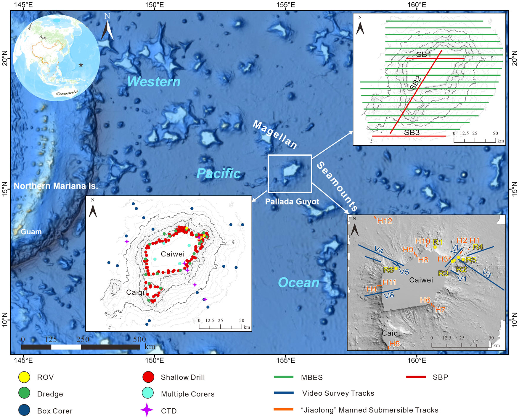
Figure 1 Overview map (source: GEBCO_2021) and survey data of the Pallada Guyot.
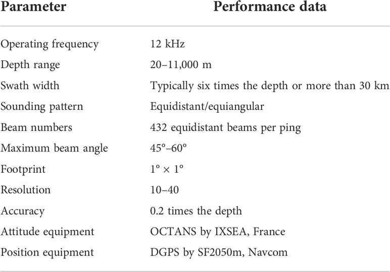
Table 1 Instruments and parameters for seabed mapping.
MBES bathymetric and backscatter data were processed with CARIS HIPS & SIPS (v.10.0, Teledyne), and a resolution of 25 m was generated according to the actual data density. Additional steps, including raw data decoding, georeferencing, radiometric corrections, angle dependence removal, pre-mosaicking corrections, and mosaicking (Yang et al., 2020), were used to process the MBES backscatter data, through which noise and external interferences were removed by filtering with manual intervention to generate a final 25 m × 25 m-resolution backscatter mosaic image.
A total of 168 surficial sediment samples, including 18 corer samples (GH-Box50 box corer, 50 cm × 50 cm × 80 cm in size), 122 shallow drills (DY-QZ150 sub-bottom drill system, with a maximum drill depth of 1.5 m; the upper-60-cm samples were used), 20 dredge samples (2.2 m × 0.7 m in size), and four multiple corers, were collected from 2004 to 2020. All samples were analyzed according to China’s National Marine Geology and Geophysics Survey specifications (GB T 12763.8-2007). For the videos and images, six videos were taken by the Guangzhou Marine Geological Survey’s “HAI MA”, a remotely operated vehicle, and the GQSX-6000 video recording system; nine photographic transects were carried out using a deep-towed imaging system from 2007 to 2012, and 12 camera sleds were taken by the “JIAO LONG” manned submersible from 2013 to 2014. All transects were taken across the contours from the top of the guyot to the slope area, which incorporates high-definition video and still camera systems using an ultrashort baseline positioning system (USBL, with a precision of 1 m, Kongsberg HiPAP 100) for underwater positioning (Figure 1).
Terrain attributes and structure classification
Terrain attributes such as seafloor slope and bathymetric position index (BPI) at fine and broad scales, which are derived from bathymetric data, can be used as proxies for habitat studies (Bouchet et al., 2015; Bargain et al., 2018; Linklater et al., 2019). The slope is not only a fundamental characteristic of the seafloor but also an important factor affecting the local current and erosion rate (Goes et al., 2019). BPI is a measure of where a digital bathymetry model (DBM) focal cell is relative to the average elevation of surrounding cells (Erdey-Heydorn, 2008; Jerosch et al., 2015; Shaun Walbridge et al., 2018). Positive values of BPI denote features higher than the surroundings, such as ridges, while negative values denote features lower than the surrounding area, such as valleys. In addition, BPI values close to zero indicate either flat or constant-slope areas.
Different scales of BPI are used to identify fine or broad benthic features, and trial-and-error methods are used to determine the most suitable scale factor. Following Lundblad et al. (2006), the BPI scale factor is the outer radius multiplied by the bathymetry resolution. Scale factors of 25 (24 outer radius and three inner radius) and 80 (80 outer radius and 20 inner radius) were chosen to create the final fine- and broad-scale BPI grids, respectively. In our study area, the small features (distance between relatively small ridges of the flank) are approximately 600 m across, whereas the large features (e.g., the distance across large flats, local depressions, and gentle slopes) are approximately 2,000 m across. BPI is given in grid units, which are standardized by subtracting the mean value of the BPI data from each BPI data point and dividing by the standard deviation. Thus, the BPI data point has a value of 0, and the standard deviation has a value of −1/+1. The standardized value of each data point was then multiplied by 100 (Wienberg et al., 2013). Slope values of 5° and 45° were selected as the slope class breaks based on natural breaks in the dataset and expert judgment after several trial-and-error runs (Erdey-Heydorn, 2008). As shown in Figure 2, the criteria for defining the structure classes are based on ensemble analysis, including DBM, broad- and fine-scale BPIs, and slope. The BTM module, as an extension of ArcGIS (version 10.4), was used to derive all of the above-mentioned attributes (Wright et al., 2005).
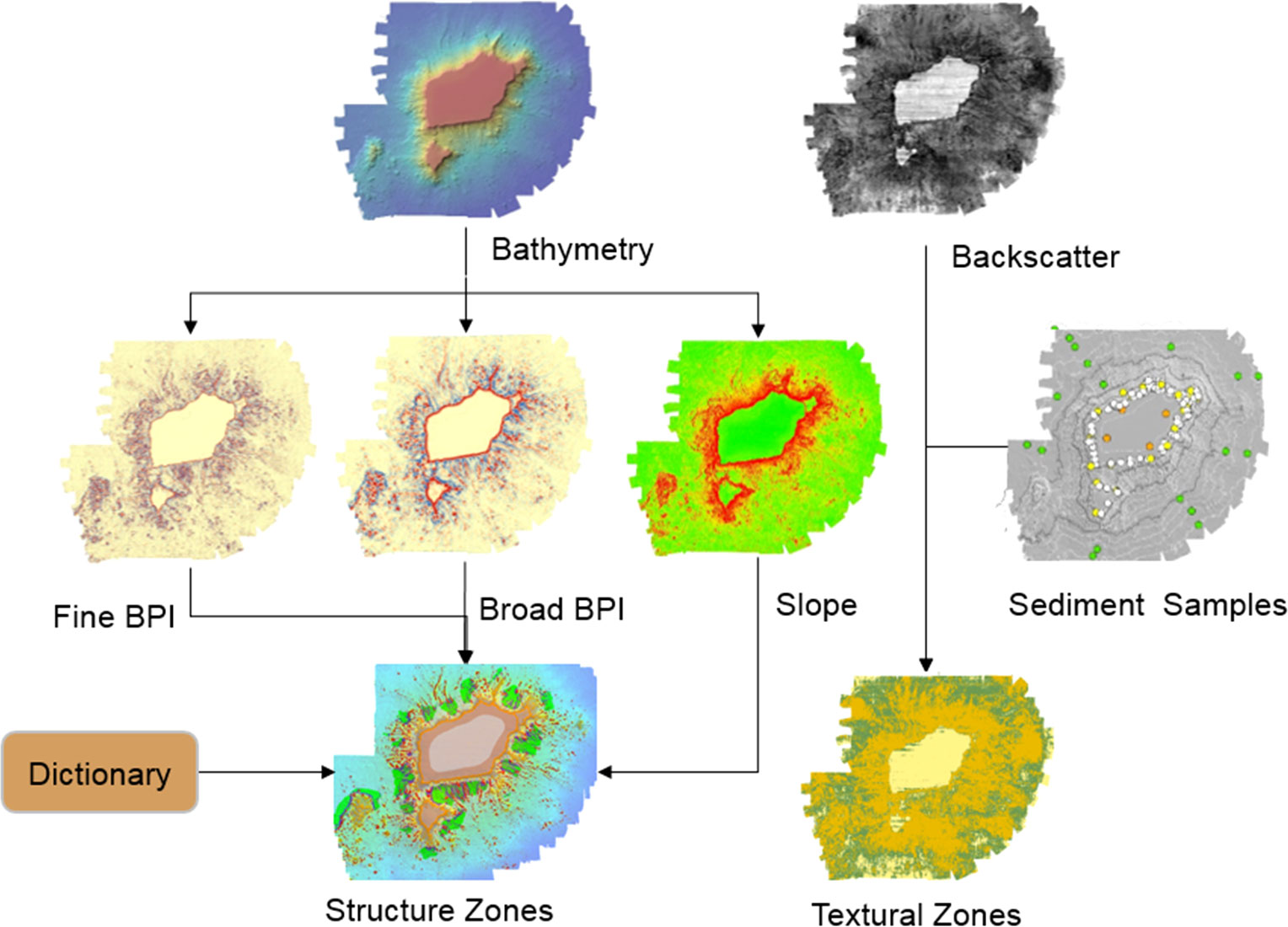
Figure 2 Flow chart of the structural zone and textural zone classifications.
A decision table with 13 structural zones, as shown in Table 2, was applied to classify the benthic structures from steep to depression in the study area. Zones 1–7 describe elevated topographic structures such as outcrops, ridges, and boulders, whereas zones 8–13 are flat and extensive areas including flat tops, plains, and depressions.
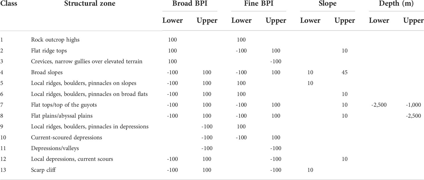
Table 2 Decision table of structures.
Multibeam echosounder system backscatter analyses and seabed classification
Acoustic backscatter data, along with ground-truthing sediment samples and towed camera video images, are widely used for habitat characterization (Craig et al., 2011; Pillay et al., 2020). According to the Coastal and Marine Ecological Classification Standard of the Federal Geographic Data Committee (FGDC-CMECS, 2012; Sowers et al., 2020), the 168 sediment samples were divided into three substrate components: mud, sand, and bedrock (Figure 3). The mud is composed of more than 90% pelagic clay; the sand is mainly foraminifera; and the bedrock is covered by more than 50% breccia, basalt, limestone, pyroclastic, volcanoclastic rock, and carbonate rocks (Table 3). Among the sediment samples, 70% were randomly selected as the training set, whereas the remaining 30% were used as the testing set for verification (Figure 3). First, 25-m buffers were created for the training sets as they only represent a small range of seabed surface sediment information. Then, the two most widely used methods in seabed textural classification were carried out to generate backscatter-based seabed classification maps: the ArcGIS™ maximum likelihood classification (MLC) and the ENVI random forest (RF) that has the latest RF classification plug-in developed by ENVI-IDL. A better result was obtained for the final textural classification. To avoid over-interpretation of the acoustic data, the zonal and textural classifications were not merged (Figure 2).
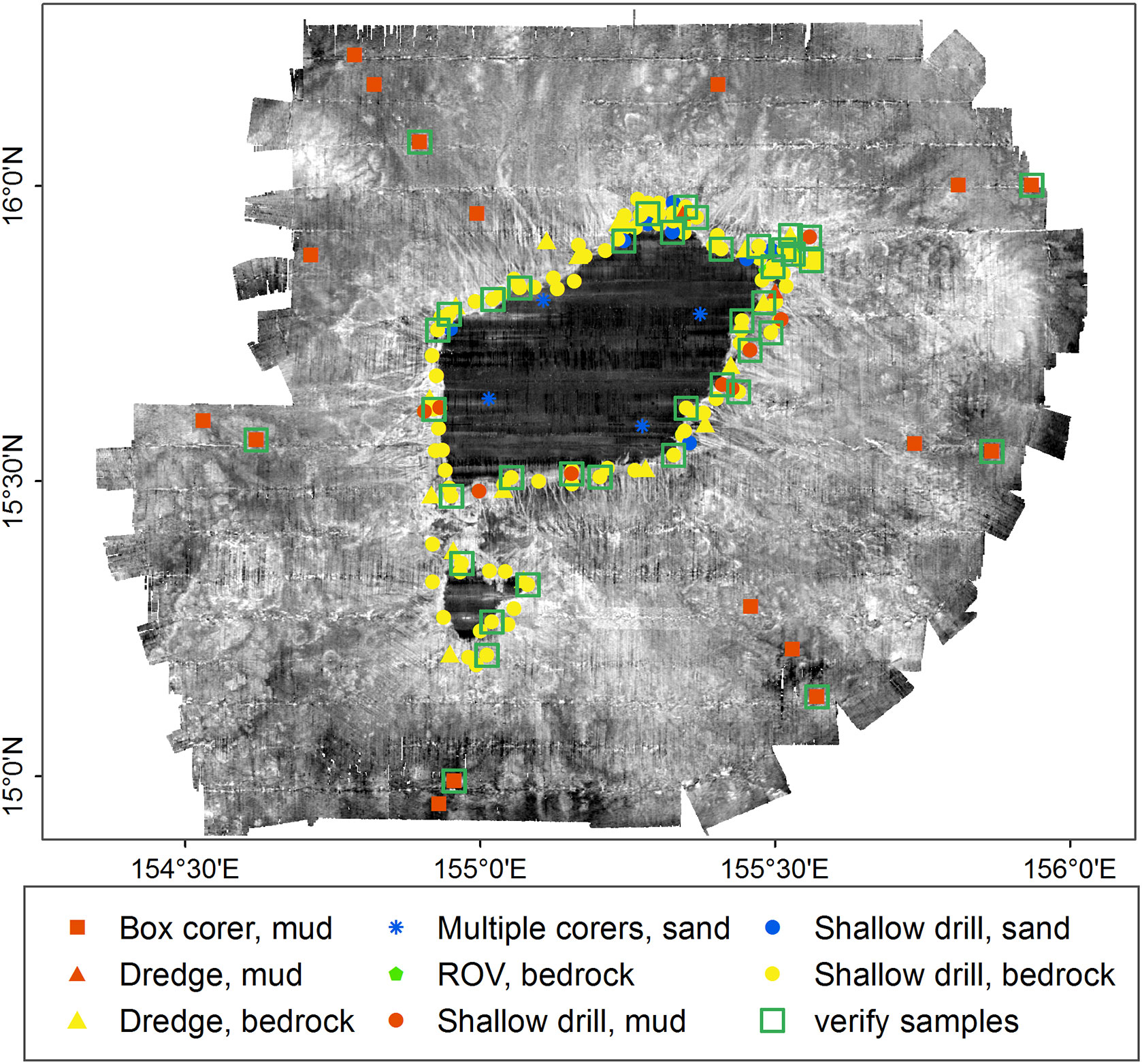
Figure 3 Backscatter mosaic image and ground-truth sampling data.
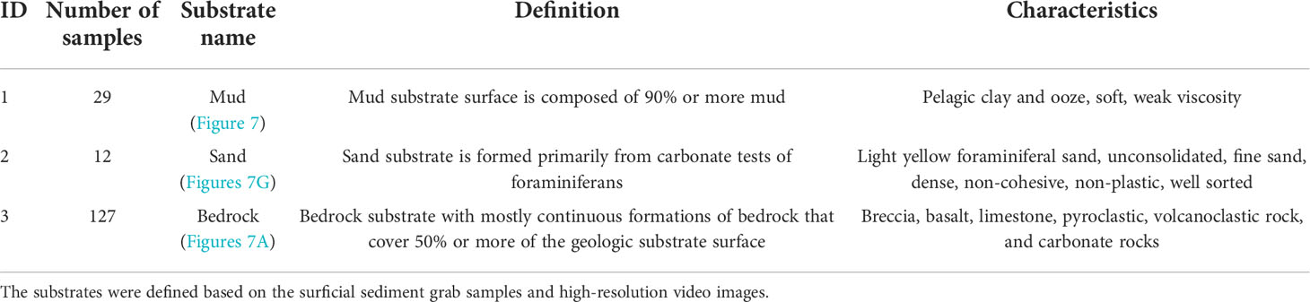
Table 3 Substrate classes defined to describe the landscape of the Pallada Guyot.
Results
Bathymetric analysis and structural zonal seabed classification
The guyot had a sub-elliptical shape with a WS elongation and two distinct flat tops. The northern flat top (Caiwei), with water depths between 1,500 and 1,650 m and an area of 1,912.2 km2, has an average slope between 0.5° and 2°. Most flanks of Caiwei, except the northwest, had steep slope maxima of more than 30° and canyon-like structures. In contrast, the other southern flat top (named Caiqi), with an area of 125.3 km2, gradually declined to water depths of 1,850–1,900 m. The western flank of Caiqi was steeper, with several canyon-like structures, while the eastern flank had a gentle slope (Figures 4C, 5A, B).
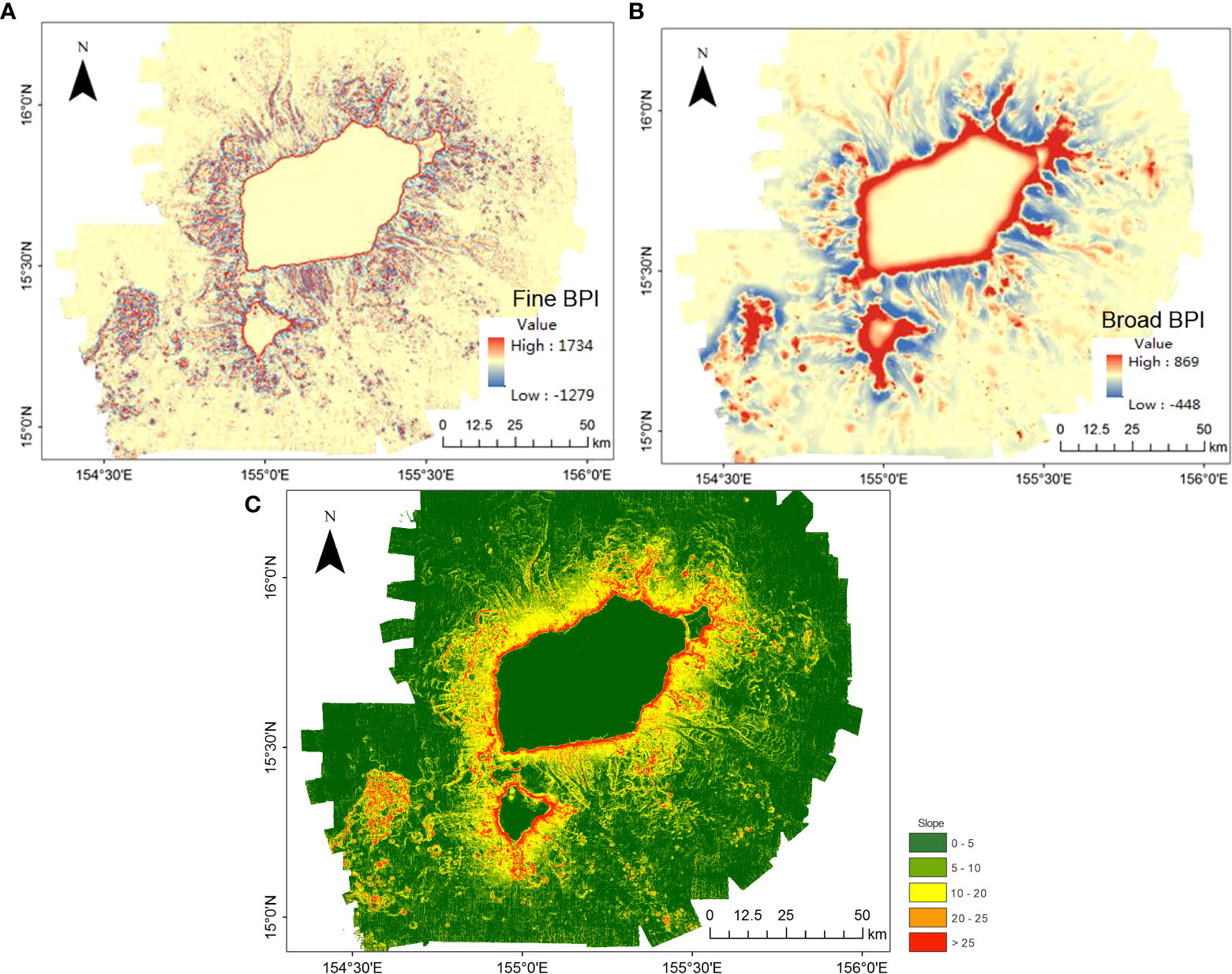
Figure 4 Bathymetric derivatives: (A) Fine-scale bathymetric position index (Fine-BPI), (B) Broad-scale bathymetric position index (Broad-BPI), and (C) slope.
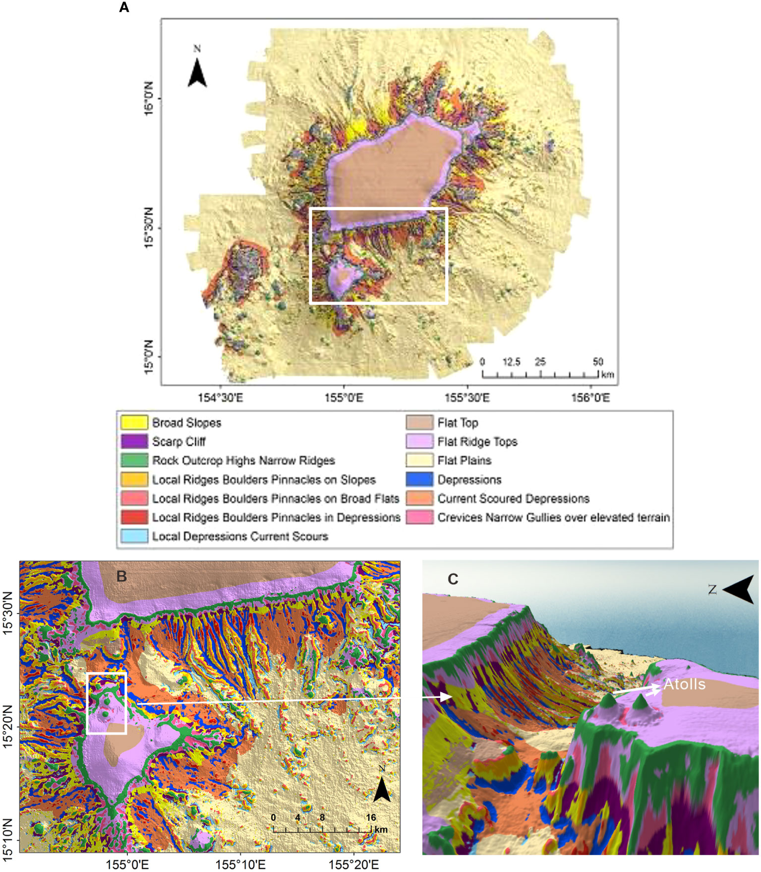
Figure 5 Structural zone classification maps: (A) structural zone classification and (B) structural zones of the southern part. The two peaks shown in the white box were inferred as the atolls. (C) 3D view of the atolls.
More details of the topographic features are revealed based on the DBM, broad- and fine-scale BPIs, and slope (Table 2). According to the results shown in Figures 4, 5, the broad-scale BPI demonstrates the major features (e.g., flat tops and depressions, Figure 4B), while the fine-scale BPI captures the subtle differences (e.g., pinnacles, local depressions, and scarps; Figure 4A). In general, the smaller the scale factor, the more detailed the features that are identified. The classification of benthic structural zones is differentiated by the BTM products, as shown in Figure 5. The percentage of each structural zone to the entire area was calculated and is shown in Table 4.
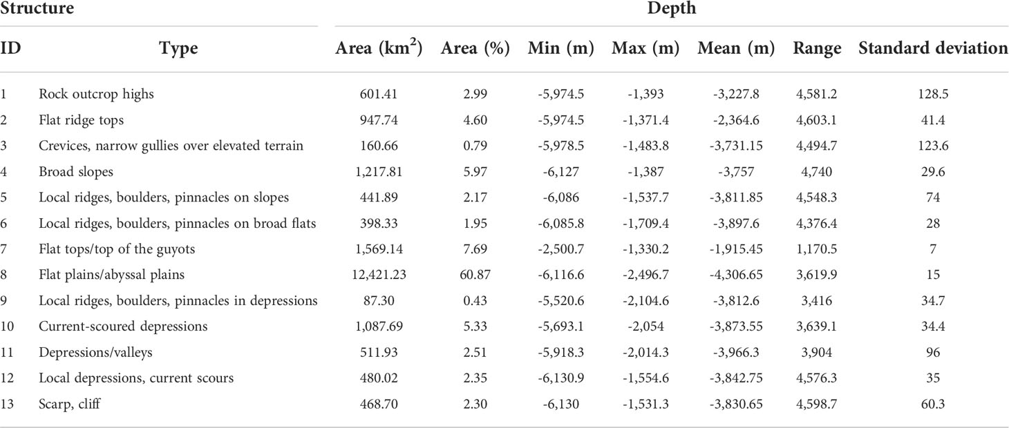
Table 4 Statistics of the geomorphological classification.
As shown in Figures 4, 5, and Table 4, the dominant structures are flat planes and flat tops, covering 68% of the study area. The classification of the structural zone reveals a more complex distribution pattern of rock outcrop highs (class 1), broad slopes (class 4), current-scoured depressions (class 10), local ridges, boulders, and pinnacles on slopes (class 5), local ridges, boulders, and pinnacles on broad flats (class 6), local ridges, boulders, and pinnacles in depressions (class 9), and depressions/valleys class 11) across the entire flank, that is, rock outcrop highs (3%) have both fine- and broad-scale features higher than their surroundings, which are distributed along the edge of the flat tops and higher bumps. Local ridges (4.5%) had narrow crests or protruding features. Depressions (2.5%) were low points on the ground, with both fine and broad features within the terrain lower than their surroundings. Local ridges and depressions indicate distinct canyons that mainly developed on the eastern and southern flanks. Broad slopes (6%) and current-scoured depressions (5.3%) were broad-scale landforms with constant slopes distributed over the entire flank. Overall, the topographic zonal seabed classification clearly shows the broad-scale landforms nested with the fine-scale topographic features of Pallada Guyot.
Multibeam echosounder system backscatter and textural seabed classification
The MBES backscatter intensity is closely related to the composition of the seafloor. Backscatter images of the seafloor classified by the MLC and RF methods are shown in Figure 6, which illustrates the general distributions of sand, bedrock, and mud. As can be seen, the image of RF is finer than that of MLC and thus has the ability to identify more detailed information, for example, relatively low-intensity areas are identified as mud on the flat top. However, sand is also a common substrate based on more than 4,200 photos from V1–V6 and H11 taken on the flat-topped area (Figures 6A, B, 7G–I, K). Moreover, after evaluating the accuracy of the verified samples (Figure 3, Tables 5, 6), the MLC, which presents an overall classification accuracy of 79.5% and a kappa coefficient of 0.43, performs better than RF, with a classification accuracy of 76.7% and kappa coefficient of 0.41.
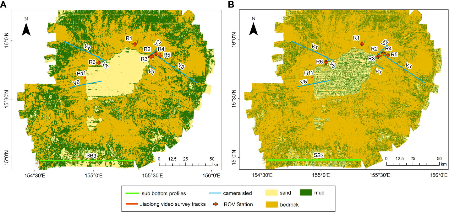
Figure 6 Textural results of the backscatter images [(the red crosses are remotely operated vehicle (ROV) stations]: (A) maximum likelihood classification. (B) Random forest classification.
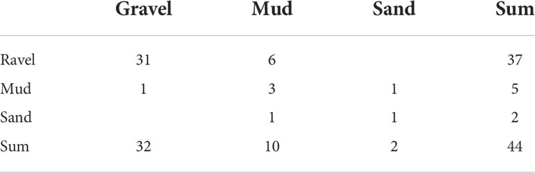
Table 5 Contingency table of the maximum likelihood classification.
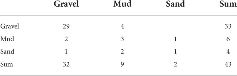
Table 6 Contingency table of the random forest.
Both the structure (Figure 5A) and textural classifications (Figure 6) show that the bedrock, which is associated with morphological highs and steep slopes, is mainly distributed on the guyot flank and dominates 50% of the study area. According to laboratory analysis, the bedrock is mainly composed of breccia, basalt, limestone, pyroclastic, volcanoclastic, and carbonate rock. Mud, which is associated with morphological flats (abyssal plains), is mainly distributed on the flat planes and accounts for 35% of the entire area, and is composed of pelagic clay and oozes. Sand, which develops mostly on flat tops (top of the guyots), covers 15% of the area and is mostly a foraminiferan-formed unconsolidated substrate.
Video images and occurrences of benthic megafauna
The megafauna on Pallada Guyot consist of benthic living species, and skeletal remnants were also observed in the video images. The still images in Figure 8 show the variety of megafauna present in the Pallada Guyot. Many corals were observed on or around high-relief crusts at station R1 (Figure 8A). Corals, starfish, sponges, fish, and shrimp appeared frequently at station R3, H3 (Figures 8B, C). However, there were fewer megafauna in R2 and R4–R6. Overall, the quantity and size of the megafauna on the shallow flat-topped and flank areas were higher than those on the deep abyssal plain. Sponges, corals, and crinoids were observed in greater numbers (Figures 8A, C, E–I), clinging to current-exposed boulders and behind sediment-sheltered overhangs of ledges.
Most of the living coral colonies grow on hard substrates, and thus the rock outcrop highs are their preferred habitat. Actinians, sea cucumbers, starfish, and crustaceans live on flat and unconsolidated substrates (Figures 8B, D, J).
Discussion
Sedimentological and morphological features of the Pallada Guyot
The exposed bedrock associated with slab crusts (Figures 7B, C, E), gravelly crusts (Figures 7A, L), or a mixture of these (Figures 7C, F, G), is dominant at the flank of the Pallada Guyot. The flank was revealed to have a more complex distributed pattern of rock outcrop highs, local ridges, and depressions (Figure 5B), indicating that it was scoured by high-speed currents. Ma et al. (2013) concluded that the bottom currents of conical seamounts change regularly from strong to weak, whereas the currents of flat-topped seamounts are strongly and weakly polarized, and their activity is only prominent at the mountain top edge and flank zones (Ma et al., 2013). Our structural zonal seabed classification provides clear evidence that the distinct current-scoured depressions, valleys, and sparse sediment coverage of the flank result from a strong bottom current.
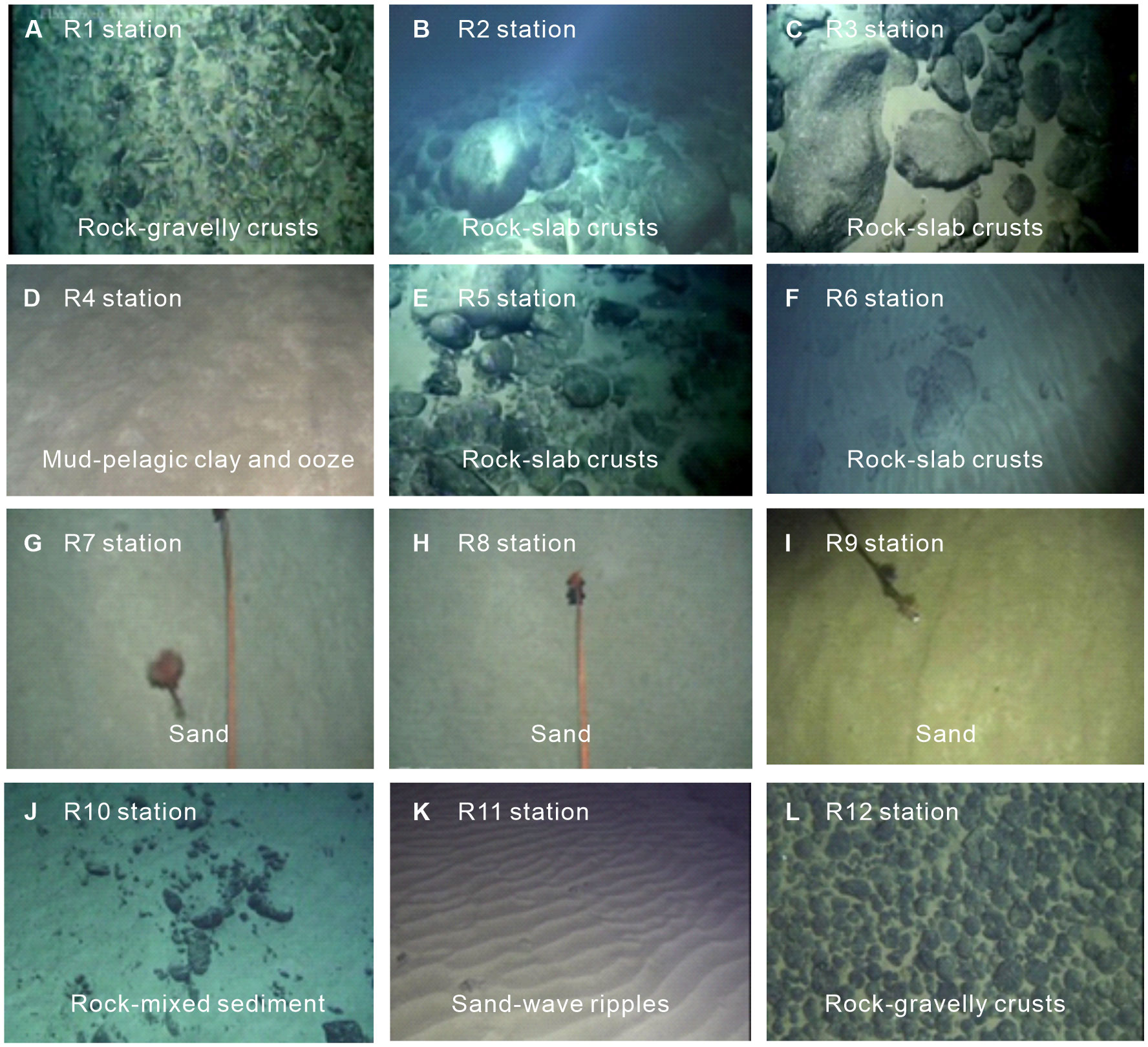
Figure 7 Still images of substrate. (A) and (L) show Rock- gravelly crusts appearance on R1 and H12. (B), (C), (E), (F) show Rock- slab crusts appearance on R2, R3, R5, R6. (D) shows the Mud- pelagic clay and ooze on R4. (G–I) show sand substrate on Flat top areas of V2, V5 and V6. (J) shows the Rock- mixed sediment on lower slope area of H9. (K) shows Sand-wave ripples on Flat top area of H11.
Sand is mainly distributed on the flat tops as well as on the southern part of the flat plains. Sediment sample analysis and video images (Figures 7G–I, K, 8B, J) demonstrate that it is unconsolidated foraminiferal sand (Xu, 2021). Moreover, the sub-bottom profile data (Figure 9) indicate that the sediment layer at the top of the guyot (Caiwei) with a thickness of more than 75 m, which spreads in the NE–SW direction, is mainly composed of foraminiferal sand. The thickness of the layer is 100–130 m in the NE, west, and SW central areas, as shown in Figure 9A, while it decreased sharply to approximately 20 m at the edge of the flat tops. The small flat top (Caiqi) is covered by the SN-direction sediment belt; the thickness decreased from 100–170 m in the central area to 10–15 m at the edge (Figure 9B). The obvious protrusion on Caiqi revealed by the sub-bottom profile SB2 shown in Figure 9B is interpreted to be a biological reef with lagoon sedimentation developing in the middle and thus, is classified as rock outcrop highs in the benthic structural zones (Figure 5B). In the southern part of the abyssal plain, the bottom profile SB3 (Figure 9C) shows that the sediment cover is discontinuous with alternating thin and thick covers, which is generally consistent with our textural seabed classification results. Figures 6A, B show that the SB3 profile area has bedrock, sand, and mud distributions. Moreover, the camera images (Figures 7C, E, F, J) show that the slab and gravelly crusts in the flank area are mainly filled with unconsolidated sediments.
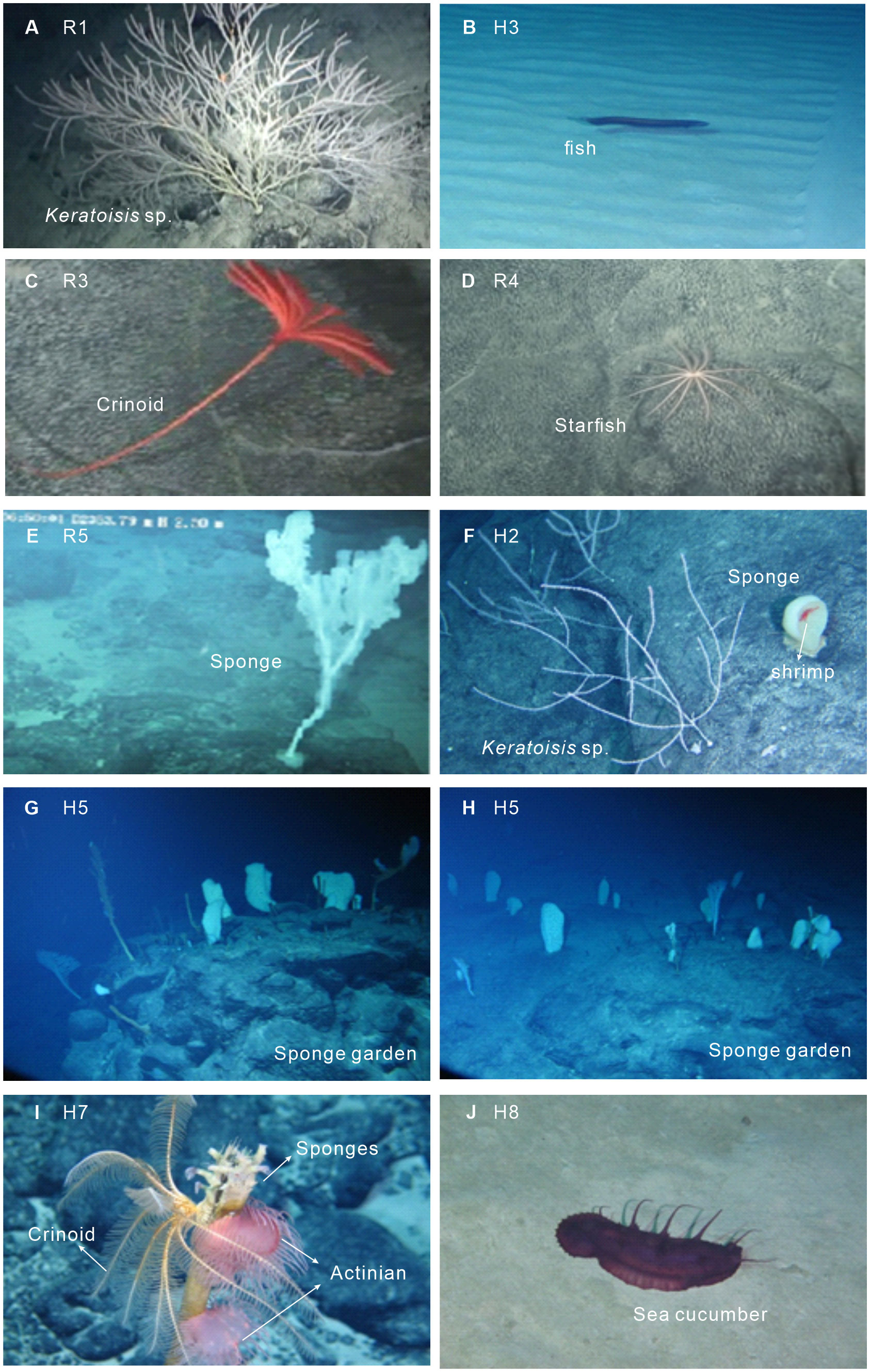
Figure 8 Still images of the megafauna: (A) Keratoisis sp. on rock outcrop highs. (B) Fish on flat unconsolidated sand. (C) Crinoid on rock outcrop highs. (D) Starfish on flat ridge tops with bedrock. (E) Actinian on crevices, narrow gullies with bedrock. (F) Keratoisis sp. and sponge on rock outcrop highs and crevices, narrow gullies. (G, H) Sponge garden on rock outcrop highs. (I) Two actinians and a crinoid attached to the sponge stem on rock outcrop highs. (J) Sea cucumber on broad slopes with unconsolidated sand.
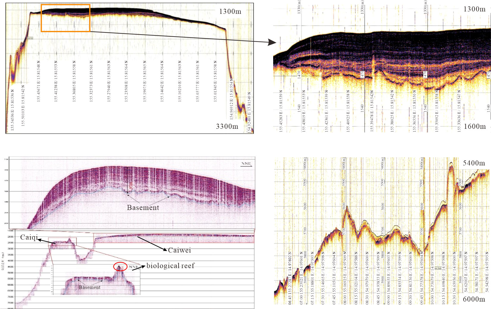
Figure 9 Images of sub-bottom profiles: (A) Sub-bottom profiles of SB1. (B) Sub-bottom profiles of SB2; the red circle shows the biological reef with lagoon sedimentation. (C) Sub-bottom profiles of SB3.
Mud mainly covers the flat abyssal plains with a general slope of less than 5°. Mud is believed to be generated by the remains of benthic and pelagic organisms because it is isolated from continental sediment input. Areas covered with mud are characterized by weak and homogeneous backscatter intensities (Yang et al., 2020). However, because the backscatter image is influenced by various factors such as slope, beam angle, and artifacts in the water column (Wienberg et al., 2013), the classification results are inconsistent with some still images, for example, our classification shows the mud result at H12, whereas gravelly crusts appear on the still image (Figure 7L). Hence, special issues including the size and accuracy of selected sample data and the ratio of the geometrical roughness to the acoustic wavelength should be considered for the backscatter classification (Lurton et al., 2015; Diesing et al., 2020).
In general, the flat tops of Pallada Guyot are covered by loose foraminiferal sand with a thickness of 100–170 m at the top and 20 m at the edge. In the flank area, the exposed bedrock with high-speed current-scoured rock outcrop highs, local ridges, and depressions is dominant. Flat abyssal plains are mainly covered by mud composed of pelagic clay and ooze deposits.
Geomorphological structure control on the benthic megafauna
The benthic megafauna in Pallada Guyot and its control factors are summarized in Table 7, in which the water depth, slope, and substrate composition were selected according to the current understanding of the drivers of the mega-epifaunal community on seamounts (Rowden et al., 2017; de la Torriente et al., 2018; de la Torriente et al., 2019; Roberts et al., 2018; Morgan et al., 2019).
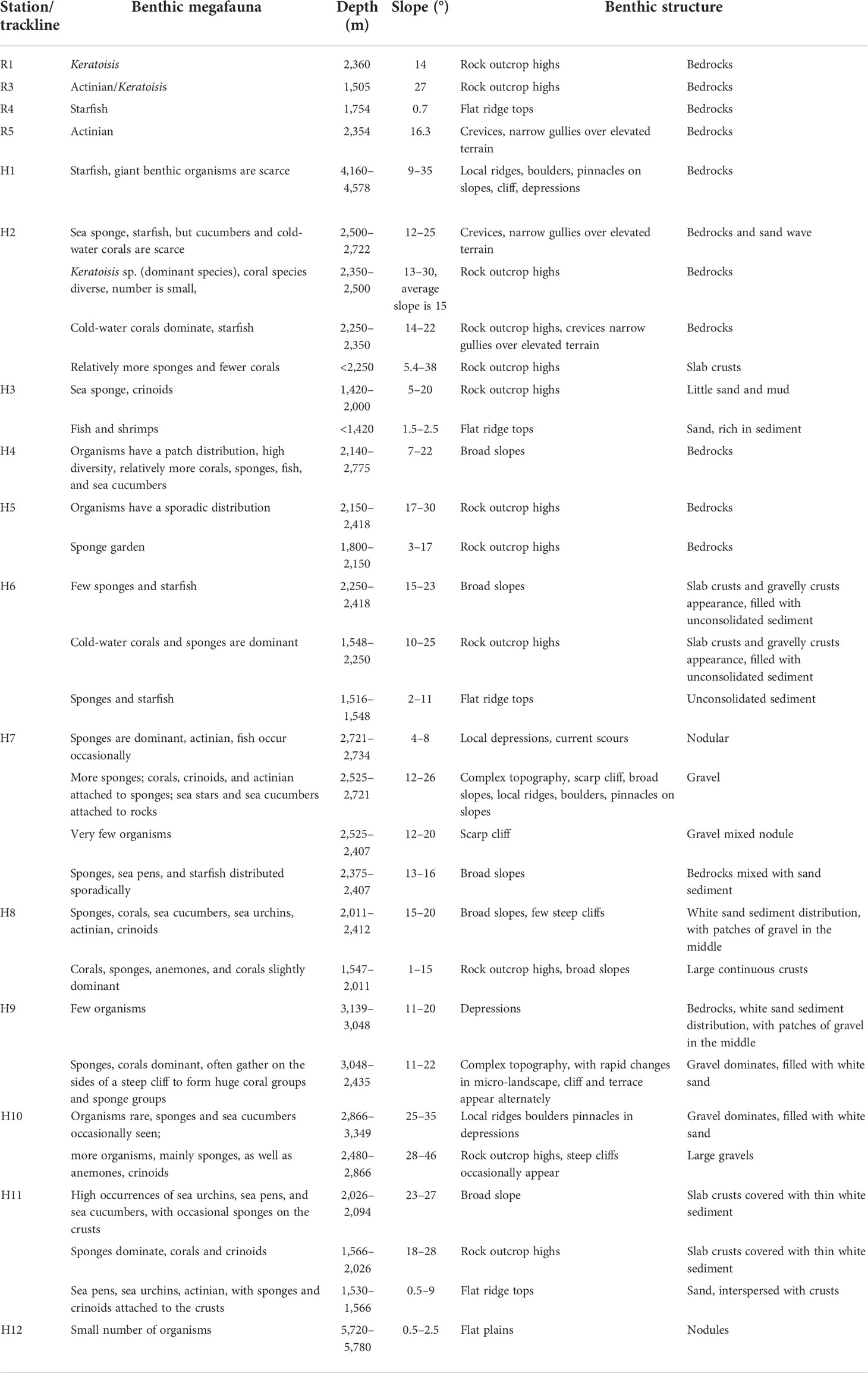
Table 7 Megafauna occurrences and related benthic structures.
Depth is commonly assessed as a key driver of faunal composition in the deep sea (Davies et al., 2015; Du Preez et al., 2016; Serrano et al., 2017; Lapointe et al., 2020; Bridges et al., 2021; Goode et al., 2021). Seamount benthic megafauna tend to be distributed in belts with depth; specifically, cold-water corals are small in size and few in number in deeper waters (Tittensor et al., 2009). Except for sporadic small sponges, gorgonians, sea stars, and sea cucumbers, a few species and a number of megafauna were observed in either the northeastern lower slope between 4,200 and 4,600 m or the northwestern plain area with water depth of 5,720–5,780 m. The number of sponges, sea stars, and corals in shallower water tended to increase as the depth increased to 2,500 m. The cold-water corals had the highest biomass within the water depth of 2,350–2,250 m, while sponges, crinoids, and anemones were dominant in areas shallower than 2,250 m. Fish, shrimp, and sea urchins were the dominant species on the shallowest flat tops. Moreover, sea stars are common at different depths, and sponges are in a greater number, especially at the flat top edges at a depth of 1,800–2,500 m, which extends the knowledge that sponge grounds occur in a marked depth belt of 2,500–3,000 m in the Northeast Tropical Atlantic (Ramiro-Sánchez et al., 2019). Thus, our work found that the distribution of megafauna in WPO seamounts is different from that in other oceans.
Topographic variables such as slope and BPI, which control the processes of hydrologic energy cycling, shelter, and exposure to energy inputs, migration, and spawning, are often identified as key drivers of benthic assemblages of the deep-sea seamount (Leverette, 2004; Davies et al., 2015; de la Torriente et al., 2018; Morgan et al., 2019). The number of benthic megafauna near the seamounts was significantly higher than that in the adjacent deep-sea flat plains. The steep flanking slope areas (10–25°) of the Pallada Guyot are typically characterized by high-speed bottom currents that can scour the seabed to the bedrock. Cold-water corals, especially Keratoisis sp., and sponges favor slopes due to the food supply carried by high-speed bottom currents. Most of the benthic structural zones in our classification are rock outcrop highs with complex topography, accompanied by high BPI and relatively high slope values. As suggested by Bridges et al. (2021), the seabed is relatively “bumpy”, with parts sitting above the surrounding areas. Areas with relatively gentle slopes, those western slopes containing stations H4, R6, H9, and H11, are mainly covered with sediments rather than rocks and crusts, resulting in a high diversity of mega-benthic species, including sponges and sediment-feeding organisms, such as sea cucumbers. Moreover, fish, shrimp, and sea cucumbers are frequently found in flat areas or depressions in the video images.
The substrate is also a driver of the distribution of benthic megafauna (Mcclain et al., 2010). The biomass of fish, shrimp, sea cucumbers, and sea urchins was higher in unconsolidated sediment areas, whereas corals, sponges, crinoids, and other sessile organisms were the dominant taxa clinging to current-exposed bedrocks. This concurs with Serrano et al. (2017), who found that a higher diversity of habitat provides filter feeders at slope rocky breaks. In slope nodular areas with thin sediment cover, fish, sea cucumbers, and sea urchins are also sporadically distributed.
Management implications
The modeling and mapping techniques used in this study provide insights into more detailed information about the geomorphological features of a seamount. Geomorphological information is crucial for predicting the distribution of the ferromanganese nodules and cobalt-rich crusts. The DA YANG expedition surveys from 2012 to 2015 found that ferromanganese crusts (FR), with an average thickness of 5.2 cm, develop at a depth range of 1,500 to 3,000 m and even up to 5,150 m. The thickest FR crust (<16 cm) is located at maximum depths (1,600–1,800 m) on the northeastern flat ridge tops. The distribution of FR is closely related to the geomorphological features, for example, ridges, uplifts, and upper platforms near the flat tops are enrichment regions of FR. Moreover, most of the bedrock in the textural seabed classification has a slab and gravelly crust appearance in the video images, providing useful information for identifying crusts. Hence, the classification of benthic structures in this study could aid in planning mineral resource survey stations in seamount areas.
This study also promotes the development of a suitable zonation plan that can protect ecosystem biodiversity in the Pallada Guyot, which could be affected by deep-water exploitation. ISA (2018) and Dunn et al. (2018) can help address threats and sustainably manage vulnerable marine ecosystems if robust evidence can be constructed based on ground truth and predictive models. The present study offers the first benthic structure for seamount biological protection, in which megafauna diversity on the western side of the guyot is higher than that on the eastern side, but the number is smaller. Fish, sea stars, sea cucumbers, and sponges are common on the western side. In contrast, corals dominate on the eastern side between 2,250 and 2,350 m. Sea pens, sea urchins, actinians, and starfish are mainly distributed on the flat ridge tops, whereas corals and sponge gardens are mainly distributed on the rock outcrop highs; in both areas, the crust thickness is generally greater than 6 cm and tends needs to be explored in the future. Deep-sea mining is likely to cause some degree of biodiversity loss (Ramiro-Sánchez et al., 2019; Heffernan, 2019). As corals and sponges can provide important ecosystem functions on the seamount, any deep-sea mining operation on rock outcrop highs should consider these vulnerable marine ecosystems. Fine sediments on the seafloor are disturbed by deep-sea mining, and the plumes of suspended particles can injure species feeding on filters and disrupt ecosystems (Ramiro-Sánchez et al., 2019). In addition, small cliffs and scarps that cannot be identified by the 25-m-resolution bathymetric model are usually observed from video images. Therefore, higher-resolution near-bottom geomorphological surveys should be carried out in areas with complex topography, such as rock outcrop highs and coral and sponge gathering places, to obtain more accurate topographic data for benthic habitat studies.
Conclusion
Seabed geological mapping has great potential in predicting the spatial patterns of benthic communities and ecosystems on isolated deep seamounts. This study uses a BTM and supervised classification of backscatter images to perform a geomorphological classification of a seamount in the WPO based on extensive hydroacoustic mapping, surficial grab samples, and video surveys. Benthic structures from the geomorphological perspective of a deep WPO seamount were classified for the first time.
The conclusions are as follows: The guyot has typical geomorphological characteristics: The flat tops are covered with 20–170-m loose foraminiferal sand and the flank area is dominated by complex and extensive topography including slab crusts, gravelly crusts, and their mixture, while the flat abyssal plains are mostly covered by mud composed of pelagic clay and ooze deposits. Our results demonstrate that depth, seafloor terrain, and substrate are drivers of mega-epifaunal community distribution at local scales of seamounts. The dominant taxon species of megafauna are sponges, which are concentrated in the southern, western, and northern high-relief bedrock flanks. Corals are the second most dominant taxa, which are distributed on the eastern and northern high-relief bedrock flanks. Moreover, corals are observed at a water depth of 2,250 m, while the sponge distributes at 1,800–2,150 m. Our work preliminarily provides a methodology framework for conducting geomorphological classification of the benthic structure of seamounts and thus draws the characteristics of typical WPO seamounts. However, analysis of the quantity of megafauna and environmental variables, such as water mass properties, current speed, and primary production, need to be further discussed in the future to determine the extent to which the same or similar environmental predictors can be applied to different guyots. Although the BTM classification method is widely used to classify different scales of topographic features, we still find that besides the ‘trial-and-error’ way, the scale factors which largely influence the results are difficult to choose.
Data availability statement
The original contributions presented in the study are included in the article/Supplementary Material. Further inquiries can be directed to the corresponding author.
Author contributions
MF: data processing, analysis, and writing. SS: formal analysis and project administration. YM: data collection and mapping. HW: review, editing, and supervision. JZ: methodology. XZ: supervision. PN: data processing. All authors contributed to the article and approved the submitted version.
Funding
Funding for this study was provided by the National Natural Science Foundation of China (grant numbers 42206200, 41930535, and 41702307).
Acknowledgments
We would like to thank all the scientists and crew of R/V Dang Yang Yi Hao, Hai Yang Liu Hao, and Xiang Yang Hong 06 teams for collecting and analyzing deep-sea data. We thank Dr. Hans Werner Schenke from Alfred-Wegener-Institut (Helmholtz-Zentrum für Polar- und Meeresforschung), who took the time to read this manuscript and gave valuable advice and suggestions. We thank Dr. X.B. He from the Third Institute of Oceanography, Ministry of Natural Resources, for his review and guidance on benthic organisms. We also sincerely thank the editor and reviewers for their constructive comments, which helped to improve this manuscript.
Conflict of interest
The authors declare that the research was conducted in the absence of any commercial or financial relationships that could be construed as a potential conflict of interest.
Publisher’s note
All claims expressed in this article are solely those of the authors and do not necessarily represent those of their affiliated organizations, or those of the publisher, the editors and the reviewers. Any product that may be evaluated in this article, or claim that may be made by its manufacturer, is not guaranteed or endorsed by the publisher.
References
Bargain A., Foglini F., Pairaud I., Bonaldo D., Carniel S., Angeletti L., et al. (2018). Predictive habitat modeling in two mediterranean canyons including hydrodynamic variables. Prog. Oceanogr 169, 151–168. doi: 10.1016/j.pocean.2018.02.015
Bouchet P. J., Meeuwig J. J., Salgado Kent C. P., Letessier T. B., Jenner C. K. (2015). Topographic determinants of mobile vertebrate predator hotspots: current knowledge and future directions: landscape models of mobile predator hotspots. Biol. Rev. 90, 699–728. doi: 10.1111/brv.12130
Bridges A. E. H., Barnes D. K. A., Bell J. B., Ross R. E., Howell K. L. (2021). Benthic assemblage composition of south Atlantic seamounts. Front. Mar. Sci. 8. doi: 10.3389/fmars.2021.660648
Clark M. R., Rowden A. A., Schlacher T., Williams A., Consalvey M., Stocks KI, et al. (2010). The ecology of seamounts: structure, function, and human impacts. Annu. Rev. Mar. Sci. 2, 253–278. doi: 10.1146/annurev-marine-120308-081109
Coiras E., Lo Iacono C., Gracia E., Danobeitia J., Sanz J. L. (2011). Automatic segmentation of multi-beam data for predictive mapping of benthic habitats on the chella seamount (North-Eastern alboran Sea, Western Mediterranean). IEEE J. Selected Topics Appl. Earth Obs. Remote Sens. 4 (4), 809–813. doi: 10.1109/jstars.2011.2123874
Craig J.B., Smith S. J., Lawton P., Anderson JT. (2011). Benthic habitat mapping: A review of progress towards improved understanding of the spatial ecology of the seafloor using acoustic techniques. Estuarine Coast. Shelf Sci. 92(3):502–20. doi: 10.1016/j.ecss.2011.02.007
Davies J. S., Stewart H. A., Narayanaswamy B. E., Jacobs C., Spicer J., Golding N., et al. (2015). Benthic assemblages of the Anton dohrn seamount (NE atlantic): Defining deep-Sea biotopes to support habitat mapping and management efforts with a focus on vulnerable marine ecosystems. PloS One Q2 10 (5), e0124815. doi: 10.1371/journal.pone.0124815
de la Torriente A., González-Irusta J. M., Aguilar R., Fernández-Salas L. M., Punzón A., Serrano A. (2019). Benthic habitat modelling and mapping as a conservation tool for marine protected areas: a seamount in the western Mediterranean. Aquat. Conserv. Mar. Freshw. Ecosyst. 29, 732–750. doi: 10.1002/aqc.3075
de la Torriente A., Serrano A., Fernández-Salas L. M., García M., Aguilar R. (2018). Identifying epibenthic habitats on the seco de los olivos seamount: species assemblages and environmental characteristics. Deep Sea Res. Part I Oceanogr Res. Pap. 135, 9–22. doi: 10.1016/J.DSR.2018.03.015
Diesing M., Mitchell P. J., O’Keeffe E., Giacomo O. A., Montereale G., Tim Le B. (2020). Limitations of predicting substrate classes on a sedimentary complex but morphologically simple seabed. Remote Sens. 1220, 3398. doi: 10.3390/rs12203398
Dunn D. C., Van Dover C. L., Etter R. J., Smith C. R., Levin L.A., Morato T., et al. (2018). A strategy for the conservation of biodiversity on mid-ocean ridges from deep-sea mining. Sci. Adv. 4, eaar4313. doi: 10.1126/sciadv.aar4313
Du Preez C., Curtis J. M., Clarke M. E. (2016). The structure and distribution of benthic communities on a shallow seamount (Cobb seamount, northeast pacific ocean). PloS One 11 (10), e0165513. doi: 10.1371/journal.pone.0165513
Erdey-Heydorn M. D. (2008). An ArcGIS seabed characterization toolbox developed for investigating benthic habitats. Mar. Geodesy 31 (4), 318–358. doi: 10.1080/01490410802466819
Goes E. R., Brown C. J., Araújo T. C. (2019). Geomorphological classification of the benthic structures on a tropical continental shelf. Front. Mar. Sci. 6. doi: 10.3389/fmars.2019.00047
Goode S. L., Rowden A. A., Bowden D. A., Clark M. R., Stephenson F. (2021). Fine-scale mapping of mega-epibenthic communities and their patch characteristics on two new Zealand seamounts. Front. Mar. Sci. 8. doi: 10.3389/fmars.2021.765407
Halbach P. E., Jahn A., Cherkasov G. (2017). “Marine Co-rich ferromanganese crust deposits: description and formation, occurrences and distribution, estimated world-wide resources,” in Deep-Sea mining: Resource potential, technical and environmental considerations. Ed. Sharma R. (Switzerland: Springer, Cham) 65–141.
Harris P. T., Macmillan-Lawler M., Rupp J., Baker E. K. (2014). Geomorphology of the oceans. Mar. Geology 352, 4–24. doi: 10.1016/j.margeo.2014.01.011
Heffernan O. (2019). Seabed mining is coming — bringing mineral riches and fears of epic extinctions. Nature 571 (7766), 465–468. doi: 10.1038/d41586-019-02242-y
Hein J. R., Mizell K., Koschinsky A., Conrad T. A. (2013). Deep-ocean mineral deposits as a source of critical metals for high- and green-technology applications: comparison with land-based resources. Ore Geol. Rev. 51, 1–14. doi: 10.1016/j.oregeorev.2012.12.001
Hubbs C. L. (1959). Initial discoveries of fish fauna on seamounts and offshore banks in the Eastern pacific. Pacific Sci.; 13, 311–316.
IHO (2019) Standardization of undersea feature names. Available at: https://iho.int/uploads/user/pubs/bathy/B-6_e4%202%200_2019_EF_clean_3Oct2019.pdf.
ISA (2018) Maps. international seabed authority (Jamaica: Kingston). Available at: https://www.isa.org.jm/mapshttps://www.isa.org.jm/deep-seabedminerals-contractors?qt-contractors_tabs_alt¼0#qt-contractors_tabs_alt.
Ismail K., Huvenne V., Masson D. G. (2015). Objective automated classification technique for marine landscape mapping in submarine canyons. Mar. Geology 362, 17–32. doi: 10.1016/j.margeo.2015.01.006
Jerosch K., Kuhn G., Krajnik I., Scharf F. K., Dorschel B. (2015). A geomorphological seabed classification for the weddell Sea, Antarctica. Mar. Geophys. Res. 37, 127–141. doi: 10.1007/s11001-015-9256-x
JOGMEC (2020). Available at: https://www.jogmec.go.jp/english/news/release/news_01_000033.html.
Jun Ma J. S., Li X., Qidong W., Guorong Z. (2021a). Multidisciplinary indicators for confirming the existence and ecological effects of a Taylor column in the tropical Western pacific ocean, ecological indicators, Oxford, England: Marine Environment research. Vol. 127. 107777. doi: 10.1016/j.ecolind.2021.107777
Jun Ma J. S., Li X., Qidong W., Xiaoxia S., Wuchang Z., Guorong Z. (2021b). Seawater stratification vs. plankton for oligotrophic mechanism: A case study of M4 seamount area in the Western pacific ocean. (Oxford, England:Marine Environment research) Mar. Environ. Res. 169, 105400. doi: 10.1016/j.marenvres.2021.105400
Lapointe A. E., Watling L., France S. C., Auster P. J. (2020). Megabenthic assemblages in the lower bathyal (700–3000 m) on the new England and corner rise seamounts, Northwest atlantic. deep Sea research part I. Oceanog. Res. Papers 165, 165. doi: 10.1016/j.dsr.2020.103366
Lecours V., Brown C. J., Devillers R., Lucieer V. L., Edinger E. N. (2016). Comparing selections of environmental variables for ecological studies: a focus on terrain attributes. PloS One 11 (12), 1–18. doi: 10.1371/journal.pone.0167128
Leverette T. L. (2004). Predicting suitable habitat for deep water corals in the pacific and Atlantic continental margins of north America. Available at: https://www2.unil.ch/biomapper/Download/Leverette-MSc-2004.pdf.
Linklater M., Ingleton T. C., Kinsela M. A., Morris B. D., Allen K. M., Sutherland M. D., et al. (2019). Techniques for classifying seabed morphology and composition on a subtropical-temperate continental shelf. Geosciences 9 (3), 141–179. doi: 10.3390/geosciences9030141
Lundblad E., Wright D. J., Miller J., Larkin E. M., Rinehart R., Naar D. F., et al. (2006). : A benthic terrain classification scheme for American Samoa, mar. Geod 29, 89–111. doi: 10.1080/01490410600738021
Lurton X., Lamarche G., Brown C., Lucieer V., Rice G., Schimel A., et al. (2015). Backscatter measurements by seafloor-mapping sonars: guidelines and recommendations (Geo-Hab Backscatter Working Group 1–200). Available at: http://ecite.utas.edu.au/100171.
Ma W., Jin X. L., Chu F. Y. (2013). Comparing research on the cobalt –rich crusts mineralization and distribution of conical and of conical and flat-topped seamounts from the central pacific seamounts (In Chinese). Acta Oceanologica Sin. 35 (2), 90–112.
McArthur M. A., Brooke B. P., Przeslawski R., Ryan D. A., Lucieer V. L., Nichol S., et al. (2010). On the use of abiotic surrogates to describe marinebenthic biodiversity. Estuar. Coast. Shelf Sci. 88, 21–32. doi: 10.1016/j.ecss.2010.03.003
Mcclain C. R., Lundsten L., Barry J., Devogelaere A. (2010). Assemblage structure, but not diversity or density, change with depth on a northeast pacific seamount. Mar. Ecol. 31, 14–25. doi: 10.1111/j.1439-0485.2010.00367.x
Morgan N. B., Goode S., Roark E. B., Baco A. R. (2019). Fine scale assemblage structure of benthic invertebrate megafauna on the north pacific seamount mokumanamana. Front. Mar. Sci. 6. doi: 10.3389/fmars.2019.00715
Pillay T., Cawthra H. C., Lombard A. T. (2020). Characterisation of seafloor substrate using advanced processing of multibeam bathymetry, backscatter, and sidescan sonar in table bay, south Africa. Mar. Geology 429, 106332. doi: 10.1016/j.margeo.2020.106332
Ramiro-Sánchez B., González-Irusta J. M., Henry L. A., Cleland J., Yeo I., Xavier J. R., et al. (2019). Characterization and mapping of a deep-sea sponge ground on the tropic seamount (northeast tropical atlantic): implications for spatial management in the high seas. Front. Mar. Sci. 6 (278), 1–19. doi: 10.3389/fmars.2019.00278
Richer de Forges B., Koslow J. A., Poore G. C. B. (2000). Diversity and endemism of the benthic seamount fauna in the south-west pacific. Nature 405, 944–947. doi: 10.1038/35016066
Roberts E. M., Mienis F., Rapp H. T., Hanz U., Meye H. K., Davies A. J. (2018). Oceanographic setting and short-timescale environmental variability at an arctic seamount sponge ground. Deep Sea Res. Part I Oceanog. Res. Papers 138, 98–113. doi: 10.1016/j.dsr.2018.06.007
Rogers A.D. (2018). The biology of seamounts: 25 years on. Adv. Mar. Biol. 79, 137–224. doi: 10.1016/bs.amb.2018.06.001.
Rowden A. A., Anderson O. F., Georgian S. E., Bowden D. A., Clark M. R., Pallentin A., et al. (2017). High-resolution habitat suitability models for the conservation and management of vulnerable marine ecosystems on the Louisville seamount chain, south pacific ocean. Front. Mar. Sci. 4. doi: 10.3389/fmars.2017.00335
Serrano A., González-Irusta J. M., Punzón A., García-Alegre A., Lourido A., Ríos, et al. (2017). Deep-sea benthic habitats modeling and mapping in a NE Atlantic seamount (Galicia bank). Deep Sea Res. Part I: Oceanog. Res. Papers 126, 115–127. doi: 10.1016/j.dsr.2017.06.003
Shaun Walbridge S., Slocum N., Pobuda M., Wright D. J. (2018). Unified geomorphological analysis workflows with benthic terrain modeler. Geosciences 8 (3), 1–24. doi: 10.3390/geosciences8030094
Sowers D. C., Masetti G., Mayer L. A., Johnson P., Gardner J. V., Armstrong A. A. (2020). Standardized geomorphic classification of seafloor within the united states Atlantic canyons and continental margin. Front. Mar. Sci. 7. doi: 10.3389/fmars.2020.00009
Tittensor D. P., Baco A. R., Brewin P. E., Clark M. R., Consalvey M., et al. (2009). Predicting global habitat suitability for stony corals on seamounts. J. Biogeography. 36, 1111–1128. doi: 10.1111/j.1365-2699.2008.02062.x
Vincent L., Dolan. M. F. J., Micalle A., Lucieer. V. L. (2016). A review of marine geomorphometry the quantitative study of the seafloor. Hydrol. Earth Syst. 20, 38. doi: 10.5194/hess-20-3207-2016
Wienberg C., Wintersteller P., Beuck L., Hebbeln D. (2013). Coral patch seamount (NE atlantic)-a sedimentological and megafaunal reconnaissance based on video and hydroacoustic surveys. Biogeosciences 10, 3421. doi: 10.5194/bg-10-3421-2013
Williams G. C. (2011). The global diversity of sea pens (Cnidaria: Octocorallia: Pennatulacea). PloS One 6 (7), e22747. doi: 10.1371/journal.pone.0022747
Wright D. J., Lundblad E. R., Larkin E. M., Rinehart R. W., Murphy J., Cary-Kothera L., et al. (2005). ArcGIS benthic terrain modeler [a collection of tools used with bathymetric data sets to examine the deepwater benthic environment]. or. state univ. davey jones’ locker seafloor MappingMarine GIS Lab (Charleston, SC: NOAA Coastal Services Centre).
Xu K. (2021). Exploring seamount ecosystems and biodiversity in the tropical Western Pacific Ocean. J. Ocean. Limnol. 39, 1585–1590. doi: 10.1007/s00343-021-1585-9
Yang Y., He G., Ma J., Yu Z., Yao H., Deng X., et al. (2020). Acoustic quantitative analysis of ferromanganese nodules and cobalt-rich crusts distribution areas using EM122 multibeam backscatter data from deep-sea basin to seamount in Western pacific ocean. Deep Sea Res. Part I: Oceanog. Res. Papers 161, 103281. doi: 10.1016/j.dsr.2020.103281
Keywords: Benthic Terrain Modeler, deep sea, seamounts, side scan sonar, geomorphometry, benthic habitat mapping
Citation: Fan M, Shi S, Ma Y, Wang H, Zhai J, Zhang X and Ning P (2022) High resolution geomorphological classification of benthic structure on the Western Pacific Seamount. Front. Mar. Sci. 9:1007032. doi: 10.3389/fmars.2022.1007032
Received: 29 July 2022; Accepted: 14 October 2022;
Published: 10 November 2022.
Edited by:
Lorenzo Angeletti, Department of Earth System Sciences and Technologies for the Environment (CNR), ItalyReviewed by:
Jun Ma, Institute of Oceanology (CAS), ChinaZifeng Zhan, Institute of Oceanology (CAS), China
Mariacristina Prampolini, Department of Earth System Sciences and Technologies for the Environment (CNR), Italy
Copyright © 2022 Fan, Shi, Ma, Wang, Zhai, Zhang and Ning. This is an open-access article distributed under the terms of the Creative Commons Attribution License (CC BY). The use, distribution or reproduction in other forums is permitted, provided the original author(s) and the copyright owner(s) are credited and that the original publication in this journal is cited, in accordance with accepted academic practice. No use, distribution or reproduction is permitted which does not comply with these terms.
*Correspondence: Hu Wang, aHUud2FuZ0B0anUuZWR1LmNu