In-situ long-period monitoring of suspended particulate matter dynamics in deep sea with digital video images

Suspended particulate matter (SPM) plays an important role in material transport, deposition, resuspension and the function of benthic communities’ processes in deep sea. SPM concentration data is usually indirectly measured by optical/acoustic sensors. However, converting these sensors’ signal to SPM concentration is associated with a number of uncertainties, which will lead to mis-estimation of the results. Some researchers recommend combining several optical/acoustic sensors to determine SPM concentration. However, due to the lack of corresponding video images, the interpretation of significant mismatch signals recorded by different sensors is subjective. Consequently, a better understanding of long-period SPM dynamics, especially in deep sea, is still a challenge. In this study, we seek to monitor the dynamics of SPM in deep sea, by firstly obtaining in-situ digital video images at a water depth of 1450 m on the northern slope of South China Sea in 2020, and secondly developing a digital image processing method to process the in-situ monitoring data. In this method, we defined an image signal which was the ratio between the area of the SPM and that of the total image, to characterize the SPM concentration. A linear regression model of the image signal and SPM concentration was established (R^{2 =} 0.72). K-fold cross-validation showed that the performance of the model was well. We calculated the SPM concentration derived from image signal, and manually classified SPM into three distinct morphological groups. The long-period observation revealed that numerous aggregates existed in deep sea. The change of SPM concentration and morphology under hydrodynamics was synchronous. When current speed equaled to or exceeded 0.15 m/s, there was a significantly increase in SPM concentration and size. However, such increase was episodic. When current speed decreased, they will also decrease. In addition, we compared the image signal with the optical/acoustic backscattering signal, analyzed the mismatch period among these three signals. We found that the optical backscatter signal can’t accurately reflect the SPM concentration during the mismatch period. To our best knowledge, this is the first time that the in-situ digital video images were used to analyze the dynamics of SPM in deep sea.

1 Introduction

Suspended particulate matter (SPM) refers to a mixture of clay to sand-sized particles that can be detected in suspension, and that consists of minerals from physical-chemical and biogenic origin, living and non-living organic matters (Fettweis et al., 2019). In deep sea, because there is a favorable physical and chemical environment for increased coagulation rates, constituents of the SPM generally are organic-mineral or nonbiological aggregates (Gardner and Walsh, 1990; Thomsen and Gust, 2000; Arı´Stegui et al., 2009; Bochdansky et al., 2010; Verdugo and Santschi, 2010). In addition, the deep-sea environment is extremely complex, the SPM will reaggregate or disaggregate. In terms of ecosystems, the SPM are the basis of food chain, which is closely related to the function of benthic communities (Duineveld et al., 2001; García and Thomsen, 2008; Amaro et al., 2015). Understanding the dynamics of SPM in concentration and morphology is crucial for investigating the process of material transport, deposition, re-suspension and biochemical cycle (Durrieu De Madron et al., 2017; Diercks et al., 2018; Jia et al., 2019; Wang et al., 2022). Hence, it is of great significance to accurately and continuously monitor the long-period variation of SPM in deep sea.

Long-period and high frequency deep-sea SPM concentration data is typically collected indirectly with sensors, which measure either the optical or acoustic backscatter signal (Eittreim, 1984; Rai and Kumar, 2015; Haalboom et al., 2021). Converting these signals to SPM concentration need to establish an inversion model of optical/acoustic backscatter signal with the true SPM concentration by field calibrations (Holdaway et al., 1999; Neukermans et al., 2012). The true SPM concentration is calculated through gravimetric measurements of filtered and dried in-situ discrete water samples (Wren et al., 2000; Rai and Kumar, 2015). The optical and acoustic signals depend not only on the SPM concentration, but also on the inherent properties of SPM, such as the SPM size distribution and aggregation (Hatcher et al., 2001; Downing, 2006; Sahin et al., 2019), shape and composition (Ohnemus et al., 2018). Whereas, for in-situ long-period observation of deep-sea SPM, the inherent properties of SPM will change under complex hydrodynamic conditions. What’s more, it’ difficult to obtain water samples from the bottom of deep-sea at different time to calibrate the parameters of the inversion model in real time. This will make the interpretation and quantification of the responses of different signal types complicatedly, and result in mis-estimation of the SPM concentration (Fettweis et al., 2019; Haalboom et al., 2021).

Recently, digital imaging technology and image processing algorithms are rapidly developed, which can be used in SPM measurement. This technology can measure both SPM concentration and morphology. The measuring technology is more intuitive because it directly takes photos. According to different image processing methods, this technology can be grouped into two categories. The direct measurement methods conduct microscopic images on a certain volume of water, calculate the size and shape of each SPM in the image, and then estimate the SPM volume concentration either using empirical or 3D reconstruction methods (Syvitski and Hutton, 1997; Eisma et al., 2001; Graham and Nimmo Smith, 2010; Gray et al., 2010; Rai and Kumar, 2015; Ramalingam and Chandra, 2018). However, these methods are expensive and require precise in-situ imaging systems, like Video Plankton Recorder (VPR) (Davis et al., 2005) and Underwater Vision Profiler (UVP) (Gorsky et al., 2000; Picheral et al., 2010). The indirect methods, on the contrary, aim to determine the SPM concentration by analyzing specific image signals, such as the ratio between image hue and saturation (Moirogiorgou et al., 2015), the ratio of blue and red counts (Hoguane et al., 2012), or mean grey level value (Lunven et al., 2003). These methods don’t require sophisticated imaging instrument, and only use a digital camera to capture images. Recently such indirect methods were only applied in riverine environment and there was no relevant research in deep-sea environment.

This paper aims to further understand the dynamics of SPM in deep sea, solve the problem of mis-estimation of SPM concentration measurement caused by existing monitoring technologies, and explore the potential application of indirect image analysis in SPM dynamics. We obtained in-situ digital video images at a water depth of 1450 m on the northern slope of South China Sea in 2020. An indirect image analysis method was proposed to analyze the long-period dynamics of SPM in deep sea. This study is organized as follows. Section 2 describes the study area and equipment. Section 3 introduces image analysis methods and defines an image signal which is the ratio between the area of the SPM imaging area and that of the total image, to characterize SPM concentration. Section 4 analyzes and discusses the cross-correlation of different signals, establishes and validates the relationship between image signal and SPM concentration, analyzes the dynamics of SPM in concentration and morphology and reveals the dynamics of SPM under the effect of hydrodynamics. Section 5 and Section 6 gives the future outlook and conclusion respectively.

2 Field observation

2.1 Study area

The South China Sea (SCS) is one of the largest and deepest marginal seas in the western Pacific Ocean (Wang et al., 2021). The northern slope of the SCS is located between the shelf-break and the deep-sea plain of the SCS, with the water depth of 300-3700 m. The sediments on the slope are mainly argillaceous calcareous silty sand and silty clay (Luan et al., 2019). The Shenhu Submarine Canyon Group (SSCG) is one of the obvious submarine landforms in the northern slope of SSC (Su et al., 2020). The SSCG is composed of 17 NW-SE oriented slope-confined submarine canyons and acts as the primary conduits for sediment delivered from the continental shelf and upper slope to deep water sedimentary basins (Su et al., 2020; Li et al., 2022). Our study area is located at the toe of one of the SSCG. As shown in Figure 1, SH2 (19.90°N, 115.27°E) is the monitoring point, the water depth of SH2 is approximately 1450 m. During the cruise, a box corer was used to collect sediment samples in the study area. After the seafloor sediments were collected, we inserted PVC tubes into the box corer to collect short cylindrical sample which was approximately 50 cm long. The physical properties of the sample were measured in the laboratory and the results are shown in Table 1. The results indicated that the surficial sediments have high water content (ω), high saturation (Sr) and large porosity (n). The mean particle size (D₅₀) approximately equals to 0.01 mm, the sediments are fine and cohesive. In addition, X-ray diffraction experiment showed the surficial sediments are dominated by clay minerals and rich in carbon source. The hydrodynamics within the northern slope of South China Sea is characterized by strong diurnal and semidiurnal tides (Zhao, 2014). The complex topography together with the along-slope tidal currents result in the generation of internal tides (Feng et al., 2021). The water flow velocity caused by internal tides in the deep-sea continental slope can reach 0.15 m/s (Xie et al., 2018). These enhanced hydrodynamics influence water mixing near the seafloor, result in sediment and organic matter resuspension and facilitate materials along-slope transport (Liu et al., 2019; Wang et al., 2022).

FIGURE 1

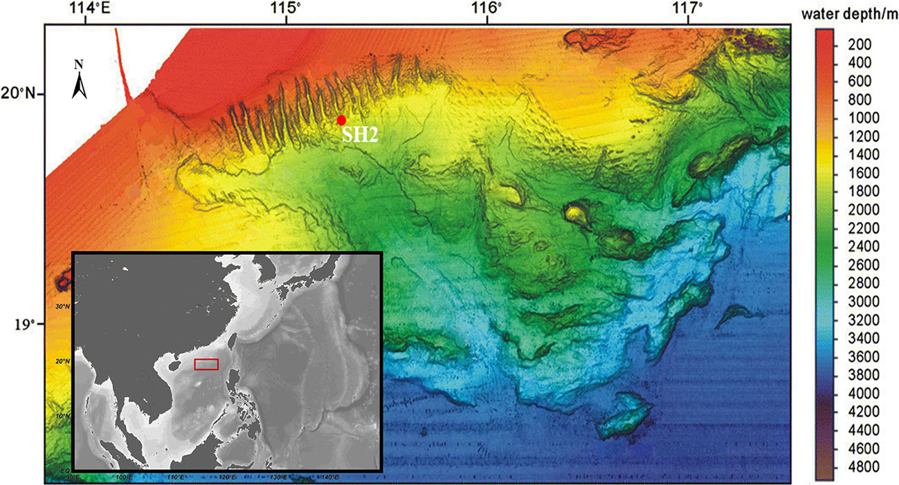
Figure 1 Geographical location (lower left inset) and the multi-beam geomorphology shadow map of the Pearl River Canyon system and adjacent area, red dot (SH2) is the monitoring point. Geographical location was mapped by Ocean Data View. The multi-beam geomorphology shadow map was modified from Ding et al. (2013).

TABLE 1

Table 1 Physical properties of surface sediments in the study area.

2.2 Equipment

The lander, shown in Figure 2A, is made of stainless steel. Its size is 3.5 m in length, 3.5 m in width and 2.7 m in height. An imaging system (to obtain video images), a Nortek Vector Acoustic Doppler Velocimetry (ADV) (to record acoustic backscatter signal and velocity), and a RBR turbidimeter (to collect optical backscatter signal), were mounted in the lander. The height above the seabed of the three instruments is 1.13, 0.6 and 0.82 m respectively. The imaging system consists of a digital video-camera, a LED light and an underwater battery. To reduce the size of the imaging system, a self-contained high-resolution (1080×1920) Charge Coupled Device (CCD) camera, and a Trans Flash (TF) card were used for video storage. The space that the camera can capture is approximately 0.6 m³. Illumination is provided by a small, low-power LED light. The total power of the system is about 18 W (3 W for the camera and 15 W for the LED light). Both the camera and the LED have the anti-pressure and anti-corrosion capacities.

FIGURE 2

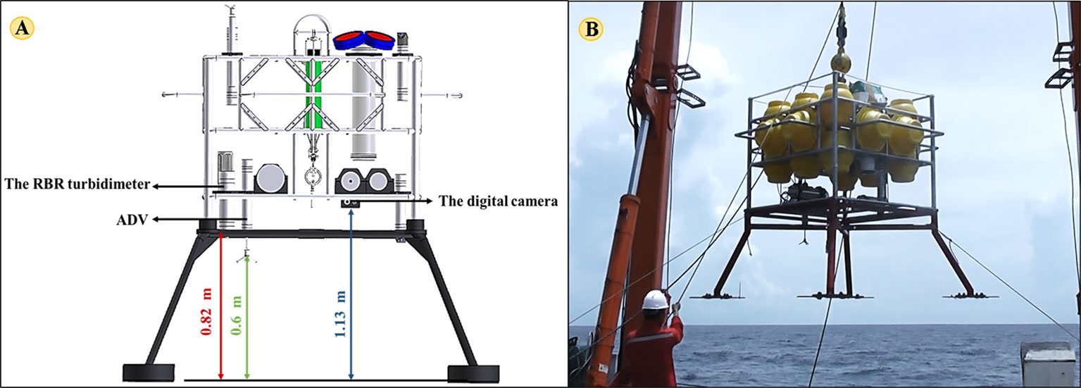
Figure 2 (A) Schematic illustration of the lander and instruments; (B) the field working picture.

2.3 Field work

The lander was deployed from the Dongfanghong3 survey vessel to the seabed on September 3^rd in 2020. It was successfully recovered by controlling acoustic releases to discard counterweight on September 23rd in 2020. The digital video-camera’s imaging rate was 30 frames per second. The video images were taken in burst for 5 s every 3 min followed by a shutdown to conserve battery and memory. The sampling frequency of the RBR turbidimeter is 1/20 Hz and that of the ADV is 16 Hz. The details of the instrument are summarized in Table 2. Each instrument is equipped with an independent, self-contained battery power supply system, enabling long time-series recordings. The field working picture is shown in Figure 2B.

TABLE 2

Table 2 Details of instrument deployments at the study area.

3 Analysis procedure for the digital video images

In order to effectively extract the image signal of the SPM concentration, a fully-automated image processing program was developed to process the deep-sea SPM video images. The video images were processed with the following four steps: (1) converting color images to grayscale images, (2) removing background, (3) converting grayscale images to binary images, (4) defining the image signal of the SPM concentration based on the processed images. The digital video image processing process is shown in Figure 3, and the specific implementation of each step is described in the following subsections.

FIGURE 3

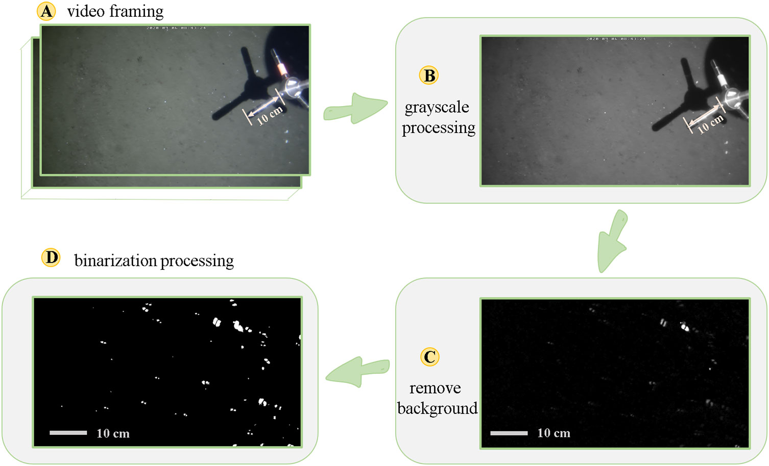
Figure 3 Digital video image processing process. (A) The original image (video framing); (B) grayscale image; (C) frame differential image, (D) binary image.

3.1 Grayscale processing

Each image after video framing was a RGB image which was stored in a 3D matrix with a dimension of “1080×1920×3” (Figure 3A). “1080×1920” denotes the total pixel number of the image and “3” denotes three channels of each pixel in red, green and blue. The first operation was to convert RGB images to grayscale images (Figure 3B). The grayscale image consists of a single channel that represents the intensity and brightness of the image (Saravanan, 2010). Converting RGB images to grayscale images will increase the data processing efficiency. Meanwhile, the precision of the results will not be affected. The function for converting RGB image to grayscale image is as follows (Bala and Braun, 2003),

$\begin{array}{ll}Gray(i,j)=0.2989*R(i,j)+0.5870*G(i,j)+0.1140*B(i,j)& (1)\end{array}$

Where Gray(i,j) is the grayscale value at the point (i,j). R(i,j)、G(i,j)、B(i,j) are the values of R, G, B components at point (i,j) in an image, respectively.

3.2 Background removing

Background removing was to distinguish the SPM information more easily. However, we found that the SPM blended into the seabed background by analyzing Figure 3B. The color feature (brightness, chroma, saturation, etc.) and texture feature of SPM were not clear enough. Hence, it is difficult to remove the background from single frame image using common algorithms, such as the image enhancement algorithm and the top-hat transform (Bai et al., 2012). In this paper, based on the moving object detection algorithm of image sequence, we successfully applied the frame difference method to remove the background (Zhao and Wang, 2007) (Figure 3C). The principle of frame difference method is as follows:

$\begin{array}{ll}{D}_k\left(i,j\right)=\left|I_k\left(i,j\right)-I_{k-1}\left(i,j\right)\right|& (2)\end{array}$

Where I_k-1(i,j) and I_k(i,j) is the k-1 and k-frame images respectively, D_k(i,j) is the difference image.

3.3 Binary processing

The images after removing the background should be converted to binary (black and white) images to extract SPM information. The process needs to define a threshold value. If pixel intensity was higher than the threshold value, they will be converted to white pixel (symbol 1) and the remaining was set to black (symbol 0). As a consequence, a binary image was a logical array with zero (black) and one (white). Setting a suitable threshold value for a large set of images was crucial to the accuracy of the processing results. Numerous automatic methods were developed to find the optimal value of the threshold. For example, Pun (1981) derived the maximum entropy method, which extracted an anisotropy coefficient from the gray-level histogram of an image. This method was closely related to its geometrical shape. Otsu (1979) provided an optimal threshold which was selected by a discriminant criterion to maximize the separability of the resultant classes in gray levels. The comparison of several threshold algorithms for images at different times is shown in Figure 4. The trail results indicated that the SPM information in the binary images segmented by maximum entropy method is generally low, whereas Otsu method is unstable. None of the automated thresholding methods were generally robust enough. In order to obtain comparable results, by trial and error, the images in this study were binarized using a constant threshold value (T=2.5), and the trail result was well.

FIGURE 4

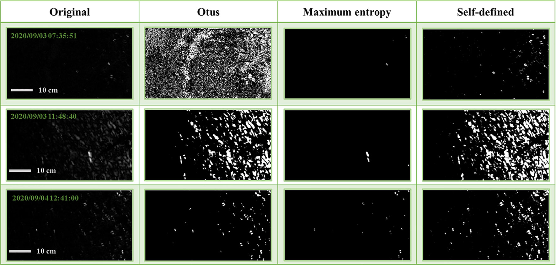
Figure 4 Comparison of threshold algorithms for images at different times.

3.4 Image signal definition

The imaging area of white spots are the main signals of the SPM concentration (e. g. the spots in Figure 3D). In this paper, the image signal of the SPM concentration is a ratio between the imaging area of white spots and the total area of each image, as shown in equation (3):

$\begin{array}{ll}{C}_i=S_{SPM}/S_{all}& (3)\end{array}$

where C_i is the image signal. S_SPM is the imaging area of white spots, S_all is the total imaging area.

4 Results and discussion

4.1 Correlation between image and optical/acoustic backscatter signal

In the last decade much work has been done to measure SPM concentration by optical/acoustic backscatter (Fugate and Friedrichs, 2002; Downing, 2006; Sahin et al., 2019). Commonly, the relationship between optical backscatter signal and SPM concentration was almost linear (Haalboom et al., 2021), and the acoustic backscatter signal was logarithmically proportional to the SPM concentration (Rouhnia et al., 2014; Öztürk, 2017; Sahin et al., 2017). In this section, we compared the image signal with the optical/acoustic backscattering signal. The time-series of image signal, optical and acoustic backscatter is shown in Figures 5A–C, respectively. We normalized the time-series of the three signals in order to compare them more intuitively in Figure 5D. The results showed that they had a similar change trend. What’s more, it’s worth noting that the optical backscatter signal has obviously different change trend from acoustic backscatter and image signal on September 5^th at16:26-September 6^rd at 00:53, which is called mismatch period (the pale pink rectangle in Figure 5). In the mismatch period, the optical backscatter signal increased by about 15 times larger than the background value, while the acoustic backscatter and image signal didn’t change significantly.

FIGURE 5

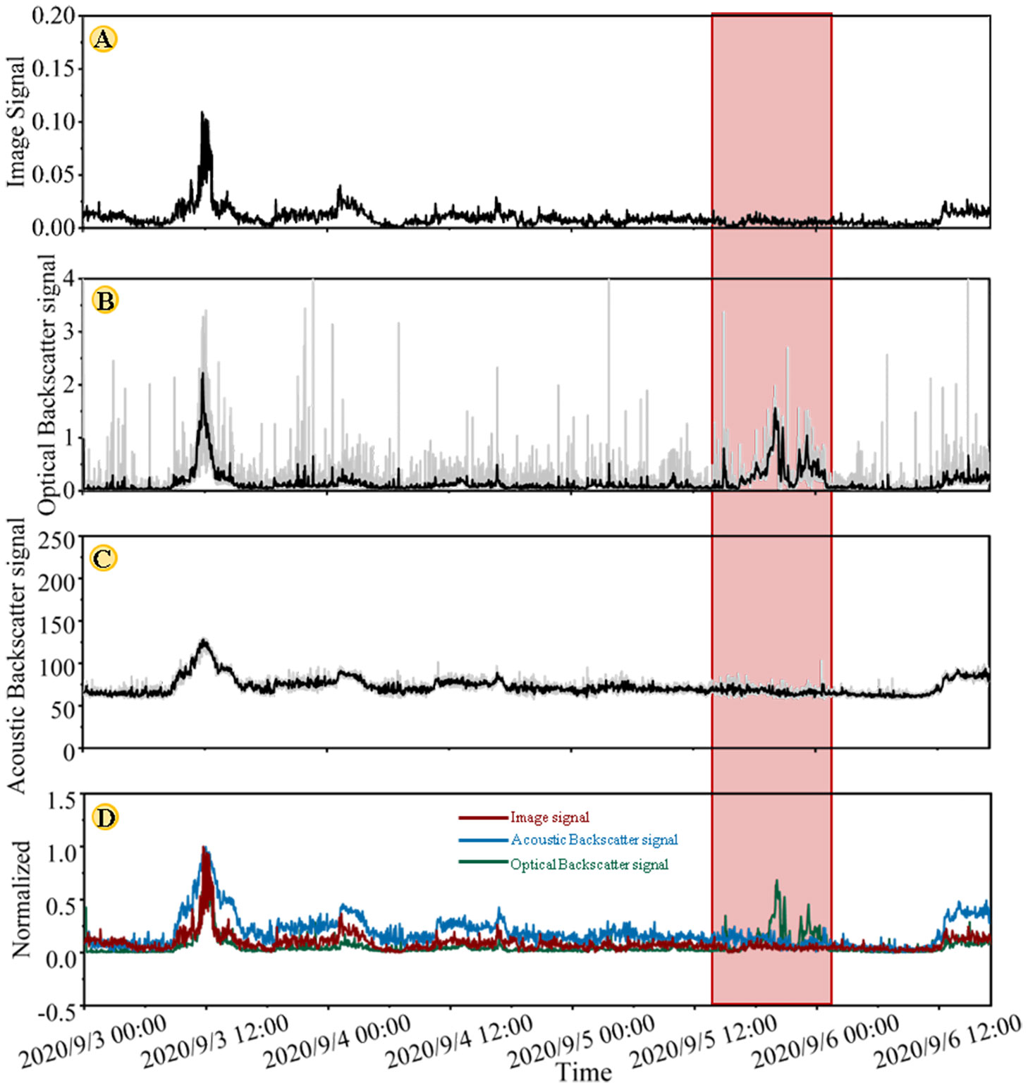
Figure 5 Near-bottom (about 1 m) time-series (September 3^rd at 00:00-September 6^rd at 17:05) at 1450 m water depth. (A) image signal recorded by digital video-camera, (B) acoustic backscatter signal recorded by ADV, (C) optical backscatter signal recorded by RBR turbidity, (D) normalized time-series. In panels (B, C), the grey lines represent the actual data, whereas the black lines represent the 3 min averaged values.

In order to quantitatively compare the image signal and optical/backscatter signal, we used normalized cross-correlation algorithm to evaluate the correlation of the three signals in the whole time-series (September 3^rd at 00:00-September 6^rd at 17:05) and the partial time-series except the mismatch period respectively. The normalized cross-correlation coefficients were calculated using the crosscorr function in Matlab using the equation 4 and equation 5,

$\begin{array}{ll}{c}_{x,y}\left(k\right)=\{\begin{array}{c}\frac{1}{n}\sum _{t=1}^{n-k}\left(x_t-\overline{x}\right)\left(y_{t+k}-\overline{y}\right) where k=0,1,2\dots \\ \frac{1}{n}\sum _{t=1}^{n+k}\left(y_t-\overline{y}\right)\left(x_{t+k}-\overline{x}\right) where k=0,-1,-2\dots \end{array}& (4)\end{array}$

$\begin{array}{ll}{r}_{x,y}\left(k\right)=\frac{c_{x,y}\left(k\right)}{S_x{S}_y} \text{where k}=0,\pm 1,\pm 2\dots & (5)\end{array}$

where x and y are the variables of the time-series to be compared (i.e., pair-wise comparison of either image signal, optical backscatter signal, or acoustic backscatter signal), t is time, x-bar and y-bar are the means of the x and y series, respectively, Sx and Sy are the standard deviations of x and y, respectively, k is the time lag, n is the sample size, Cx,y is the cross-covariance coefficient, and rx,y is the cross-correlation coefficient. The results are shown in Figure 6, when offset equaled to 0, the normalized cross-correlation was maximum and closed to 1, which meant that the image signal, optical and acoustic backscatter signal were highly correlated.

FIGURE 6

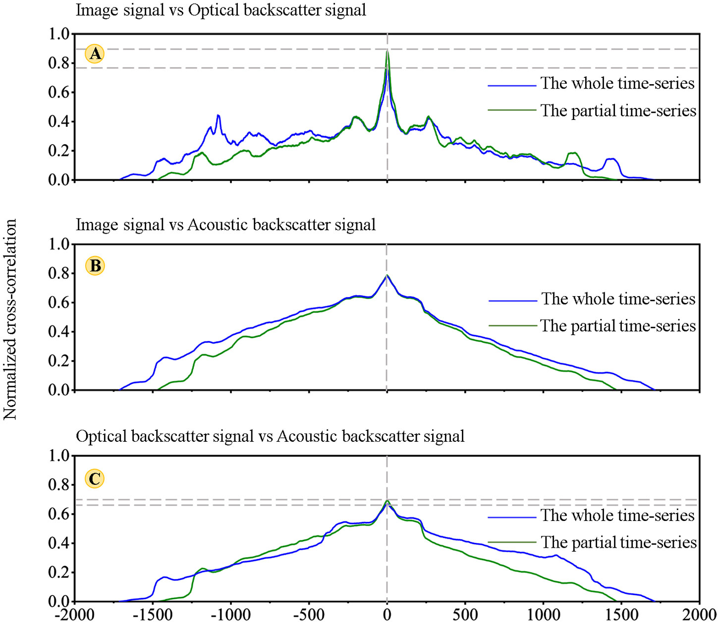
Figure 6 Normalized cross-correlation lag-time plots. (A) Image signal vs Optical backscatter signal (B) Image signal vs Acoustic backscatter signal (C) Optical backscatter signal vs Acoustic backscatter signal. On the vertical axis, values close to one indicate a higher correlation. The horizontal axis refers to the lag time between the two timeseries, negative denotes the delay between the first and second signals. The blue curve is cross-correlation analysis of the whole time-series (September 3^rd at 00:00-September 6^rd at 17:05), while the green curve is cross-correlation analysis of the partial time-series (except September 5^rd at 16:26-September 6^rd at 00:53).

However, as shown in Figures 6A, C, the correlation of the partial time-series (the green curve) was higher than the whole time-series (the blue curve). Comparing the video images during the mismatch period with the other period, we found that there was no large amount of SPM in the video images during the mismatch period. The sudden increase in optical backscatter during the mismatch period may be induced by the following three reasons: (1) in the mismatch period the majority of suspended particles were fine particles. The RBR turbidimeter was most sensitive to fine particles (Downing, 2006; Haalboom et al., 2021; Sabine et al., 2022). While these fine particles can’t contribute significantly to SPM weight (D'sa et al., 2007; Sabine et al., 2022). (2) the RBR turbidimeter only measured the signal of a single point, which may not be a representative of SPM concentration in whole study volume (Rai and Kumar, 2015); (3) biofouling or other type of fouling resulted in a temporary increase of the optical backscatter signal (Delauney et al., 2009; Fettweis et al., 2019). The above analysis showed that the optical backscatter signal can’t accurately reflect the SPM concentration during the mismatch period. Therefore, sometimes converting the optical backscatter into SPM concentration by an inversion formula will result in an overestimation of SPM concentration.

4.2 Relationship between image signal and SPM concentration

It is difficult to obtain discrete water samples at 1 m above the seabed. Thus, before recovering the lander, we collected seawater at different water depths (50, 100, 150, 200, 300, 400, 500, 600, 800, 1000, 1282, 1332 and 1372 m) by a deploying a SeaBird 911 CTD-Rosette system, and obtained the corresponding optical backscatter signal recorded by the RBR turbidimeter mounted on the CTD at the same time. We calculated the SPM concentration through gravimetric measurements of filtered and dried water samples, and then established the relationship between the optical backscatter signal and the SPM concentration (mg/L). The result is shown in equation (6),

$\begin{array}{ll}Y=4.03X+0.71& (6)\end{array}$

Where Y is the SPM concentration, X is the optical backscatter signal.

The equation was used in this study to calculate the SPM concentration during September 3^rd at 00:00-September 6^rd at 17:05. Based on the discussion in Section 4.1, the SPM concentration quantified by optical backscatter signal was overestimated during the mismatch period. Hence, we use the partial time-series to establish the relationship between image signal and the SPM concentration. We conducted linear regression analysis on these time-series. The image signal and the SPM concentration were taken as the independent and dependent variable respectively (Figure 7). The results showed that they had a strong linear relationship. The correlation coefficient R² was equal to 0.72. And a linear regression model was obtained: y=55.49 x +0.68.

FIGURE 7

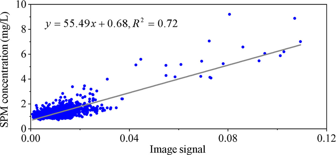
Figure 7 The relationship of image signal versus the SPM concentration.

K-fold cross-validation algorithm was used to evaluate the performance of the linear regression model (Le et al., 2022). Two evaluation indexes, including root-mean-square error (RMSE) and relative error (RE), were used to measure the deviations of the results (Wang et al., 2012; Ciancia et al., 2020; Kwong et al., 2022), which are described by equation (7) and (8).

$\begin{array}{ll}RMSE=\sqrt{\frac{{\sum }_{i=1}^n{\left(x_{i,r}-x_{m,r}\right)}^2}{n}}& (7)\end{array}$

$\begin{array}{ll}RE=\frac{{\sum }_{i=1}^n\left|\frac{x_{i,r}-x_{m,r}}{x_{m,r}}\right|}{n}& (8)\end{array}$

where x_i,r is the modeled value of the ith element, x_m,r is the SPM concentration of the ith element, and n is the number of test data set.

In order to realize the k-fold cross-validation algorithm, we shuffled the sets of “image signal-SPM concentration” data randomly and divided the dataset into 5 groups. For each group, we took this group as a test data set and the remaining groups as a training data set. We fitted the model on the training set and evaluated it on the test set. The performance of the linear regression model was evaluated with the index RESE and RE and the results were summarized in Table 3. The results showed that the RMSE was small and the RE was within ±25%, which indicated high confidence in the model-predicted values. That is to say, the performance of the model was well.

TABLE 3

Table 3 Values of RMSE and RE.

4.3 The dynamics of SPM concentration based on image signal in deep sea

We applied the established linear regression model to whole time-series of image signal to calculate the SPM concentration. The current regime presented in Figures 8A, B showed diurnal and semidiurnal variation in current speed and direction. The current velocity ranged from 0.015 to 0.27 m/s. Figure 8C showed that the background concentration of SPM at the observation station was 1 mg/L. The SPM concentration reached the peak value when current velocity equaled to or exceeded 0.15 m/s. Significant increase in SPM concentration, occurred on September 3^rd at 07:26-15:02, September 3^rd at 18:01-September 4^rd at 05:07, and September 6^rd at 11:48-17:05, which were labelled by buff rectangle I, II, III respectively in Figure 8. Particularly, for the period I, the SPM concentration was 1.08 mg/L on September 3^rd at 8:00. Then it gradually increased to the maximum (6.62 mg/L) on September 3^rd at 11:48. At this time, the current velocity reached to the maximum (0.27 m/s). Subsequently, the SPM concentration gradually decreased to the minimum (0.98 mg/L) on September 3^rd at 16:13. Within this more than 8 h interval the SPM concentration increased by 6-7 times larger than the background value (the SPM concentration is 1 mg/L). The SPM concentration variation was coincided with current velocity variation. For the period II, III, the SPM concentration increased by 2 times larger than the background value. The SPM concentration reached to the maximum when the current exceeded 0.15 m/s.

FIGURE 8

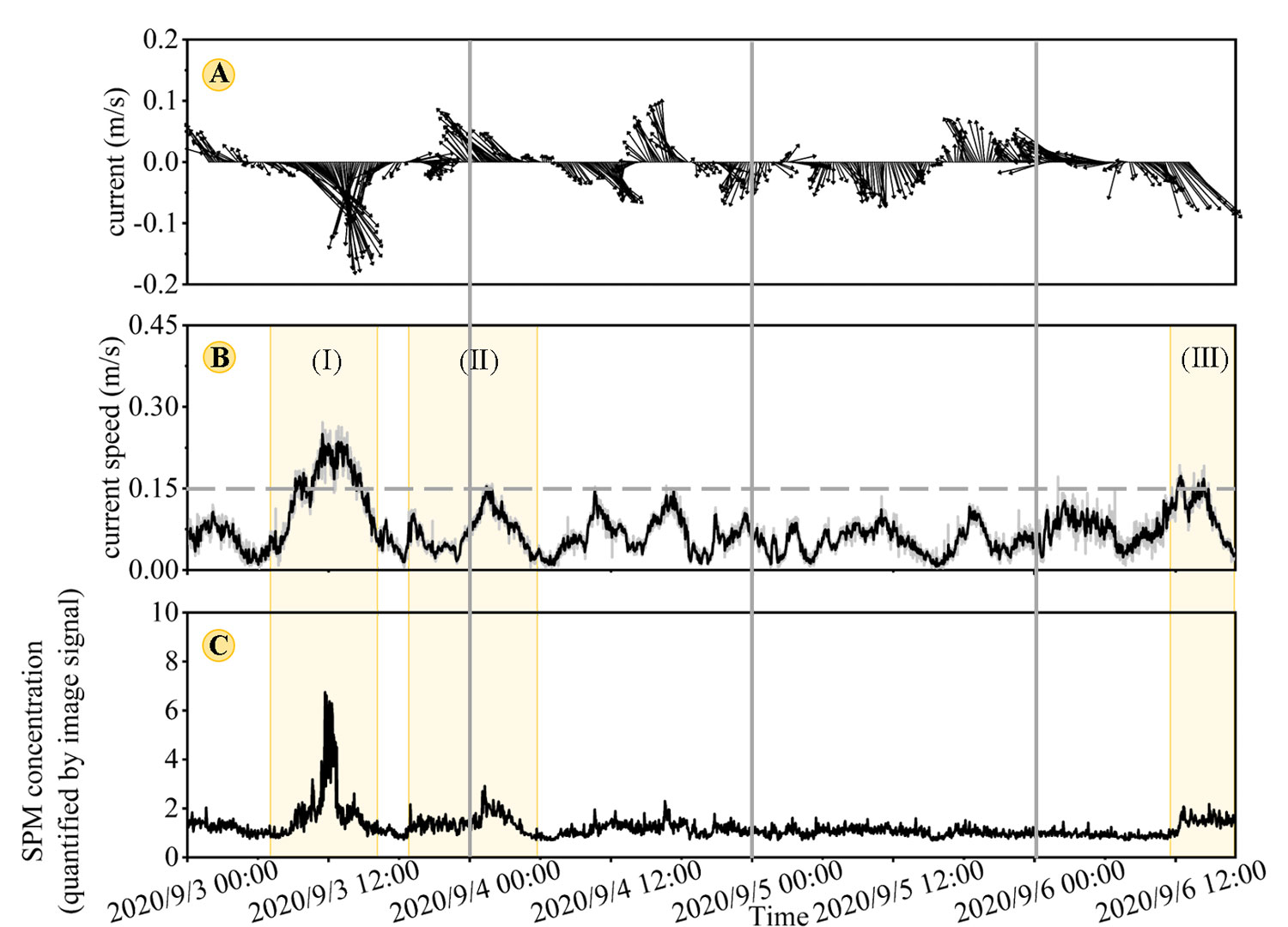
Figure 8 Near-bottom (about 1 m) time series on September 3^rd at 00:00- September 6^rd at 17:05 (A) current vector; (B) current speed (the gray dashed line indicates the threshold current when sediments resuspension occurred) (Thomsen and Gust, 2000; Xie et al., 2018) (C) SPM concentration quantified by image signal.

Combined with the physical properties and composition of the surficial sediment in the study area (described in Section 2.1), we inferred that the current speed is not strong enough to resuspend fine and cohesive sediments during the period of observation, but resuspend the fluffy organic-mineral aggregates which were on top of these more cohesive sediments. This conclusion is consistent with the results that Thomsen and Gust (2000) and Thomsen et al. (2002) developed by doing resuspension experiments with natural deep-sea sediments.

4.4 The dynamics of SPM morphology based on images in deep sea

We can directly observe the morphology of the SPM with digital video images. The observation results indicated that the SPM was mainly large aggregates in images. We manually classified them into three distinct morphological groups according the shape and size of SPM (Figure 9). In the first group, the shape of SPM was ellipse and the size was large (Figure 9A), such SPM mainly existed during September 3^rd at 07:26-15:02 (labelled by buff rectangle I in Figure 8). In the second group, the shape of SPM was circular and the size was moderate (Figure 9B), such SPM existed during September 3^rd at 18:01-September 4^rd at 05:07 (labelled by buff rectangle II in Figure 8), and September 6^rd at 11:48-17:05 (labelled by buff rectangle III in Figure 8). At other time, the SPM was dot-shaped and the size was small (Figure 9C), we named them the third group. Trudnowska et al. (2021) classified marine particles into five morphotypes by analyzing the properties of individual particles based on images taken by Underwater Vision Profiler, including circular, elongated, flake-type, fluffy, agglomerated forms of multielement structure. However, in this study, because our imaging system provided a relatively large field of view measuring and can’t supply the depth information of each particle, we can’t make precise classification based on individual particles. Hence, the way we analyze the SPM morphology is based on SPM relative changes in 2D images with time. Such discussion may be inaccurate, whereas the aim of this study is not to classify the morphology of particle perfectly but to better understand the dynamics of SPM combined with hydrodynamic information.

FIGURE 9

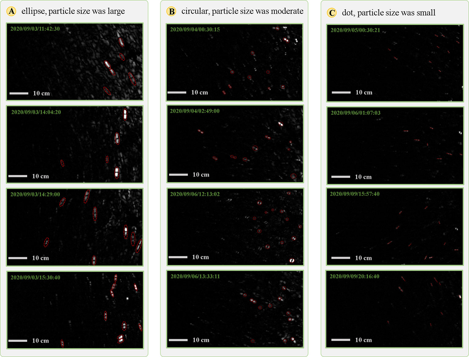
Figure 9 The typical images about three morphological groups of the SPM. (A) the first group, the shape of SPM was ellipse and the size was large, (B) the second group, the shape of SPM was circular and the size was moderate, (C) the third group, the SPM was dot-shaped and the size was small.

Haalboom et al. (2021) speculated the type of SPM under different hydrodynamic conditions according to comparing the time-series of optical backscatter signal (recorded by turbidimeter) and acoustic backscatter signal (recorded by 75 k ADCP) in Whittard Canyon at a water depth of 1400 m. They found that when the current speed increased (especially when the current speed increased to 0.4 m/s), the optical backscatter signal increased, whereas the acoustic backscatter decreased. Based on this finding, they inferred that high current velocity would cause larger aggregates break into dispersed smaller particles, whereas moderate current velocity made fine particles aggregate into larger aggregates. However, in their study, the optical and acoustic backscatter signals were recorded at different heights of, 5 and 45 m above the seabed, respectively. And they have no direct observational evidence (like underwater video images) to verify the conclusion. Different from their study, our digital video images gave us more direct and intuitive evidence to analyze the dynamics of SPM morphology. Our finding was different from theirs. Combined with the hydrodynamic conditions (Figure 8B), we found that high current velocity always correspond to large size of SPM. Particularly, when the current velocity equaled to or exceeded 0.15 m/s, the SPM had the largest size (Figure 9A). Whereas with the decrease of current velocity, the size of SPM was also gradually decreased. Hence, we thought the current speed in our monitoring point was not strong enough to break the large size SPM, and the low current speed made the large size SPM settle down.

5 Future outlook

The digital video camera captures a relatively large field of view, and provides a measuring volume of 0.6 m³. In such configuration, it is meaningless to define a lower limit of particle size the camera can detect. Despite this, we can roughly estimate the pixel size was 0.35 mm according to the marker of known actual size in the image, and the camera was expected to quantitatively capture particles with ESD (Equivalent Sphere Diameter) >0.7 mm. As a matter of fact, for these particles the camera can’t captured, the images as a whole still contain their information in a way of color, texture and so on. Therefore, for the measurement of SPM concentration, the method of this study is to excavate an image signal of SPM concentration by artificially designed image processing algorithms. And the results (discussed in Section 4.1) indicated that the method can effectively work in low SPM concentration in deep-sea environment. The RBR turbidimeter measures optical backscatter signal of particles suspended with particle size >0.88 μm in the water column (Mao et al., 2012). The output voltage is calibrated to turbidity in FTU. The relationship of turbidity and SPM concentration is linear in the range of 0-750 FTU, but it becomes nonlinear for turbidity higher than 750 FTU due to grain shielding effect (Downing, 2006; Mao et al., 2012). In our study, the turbidity values lower than 4 FTU, that is to say, the RBR turbidimeter can work effectively in low SPM concentration deep-sea environment. The acoustic backscatter response of ADV to different particle size is dependent on the operating frequency of the ADV (Ha et al., 2009). The most sensitive diameter of the 6 MHz ADV in this study we used is 80 μm according to scattering theory (Thorne and Hanes, 2002). From laboratory experiments, Li et al. (2019) has shown that 6 MHz ADV works in the range of 0-1000 mg/L.

In general, in the last decades, the optical and acoustic instruments have been widely applied and in deep-sea environment, and this is the reason why we compare the image signal with optical/acoustic backscatter signal. Yet optical and acoustic approach all have their own drawbacks like the analysis and discussion in Section 4.2. And in this study, the image analysis method has obvious advantages, such as it is more intuitive and contains more information which enables a more multidimensional interpretation of the dynamic changes in SPM. Whether the method can work effectively in higher SPM concentration environments remains to be further explored in the future work. In addition, in other scenes such single signal may cannot reflect all the information in the image, whereas the missing information is likely to be related to the SPM concentration. In the future, the use of convolutional neural networks, data-driven learning, and automatic computer extraction of multidimensional image information may further extend the range of work on image-based measurement of SPM concentration.

6 Conclusion

In this study, we conducted an in-situ long-period monitoring of SPM concentration and morphology at a water depth of 1450 m on the northern slope of the South China Sea with digital video images. The results are summarized as follows:

(1) We developed a novel method to process the deep-sea digital video images. In this method, we defined an image signal of SPM concentration. By doing cross-correlation analysis among image, optical and acoustic signals, we made a conclusion that in some period the optical backscatter signal can’t accurately reflect the SPM concentration, whereas image signal can overcome this shortcoming.

(2) We calculated the SPM concentration derived from image signal, and manually classified SPM into three distinct morphological groups. Combined with the hydrodynamics, long-period monitoring results revealed that the increase in SPM concentration and size coincided with distinct peak in current velocity, and the decrease in SPM concentration and size corresponded to the decrease in current velocity. Our direct observational evidence helps to make a conclusion that enhanced hydrodynamics resuspend the organic/inorganic matter on the deep-sea seabed, or transport the material from the continental slope to deep sea. Whereas, reduced hydrodynamics make the material settle down.

Data availability statement

The raw data supporting the conclusions of this article will be made available by the authors, without undue reservation.

Author contributions

HW took part in field sampling, developed the digital image processing method, analysed and interpreted the data, wrote the manuscript. CH initiated the central idea, revised the manuscript, discussed the results, contributed to the writing of part of manuscript and approved the submitted version. YJ initiated the central idea, discussed the results, provided advices for the manuscript and approved the submitted version. XF revised the manuscript, took part in field sampling, and provided advices for the manuscript. CJ took part in field sampling, contributed to the analysis of part of data. All authors contributed to the article and approved the submitted version.

Funding

This research was funded by the National Natural Science Foundation of China (No. 41831280), the Marine S&T Fund of Shandong Province for Pilot National Laboratory for Marine Science and Technology (Qingdao) (No. 2021QNLM020003-1)and the National Natural Science Foundation of China (No. 41907227).

Acknowledgments

We thank the Natural Science Foundation of China for the Open Research Cruise of the northern South China Sea (NORC2019-05, NORC2022-05). We appreciate all members for their efforts in the collection of the data in this study.

Conflict of interest

The authors declare that the research was conducted in the absence of any commercial or financial relationships that could be construed as a potential conflict of interest.

Publisher’s note

All claims expressed in this article are solely those of the authors and do not necessarily represent those of their affiliated organizations, or those of the publisher, the editors and the reviewers. Any product that may be evaluated in this article, or claim that may be made by its manufacturer, is not guaranteed or endorsed by the publisher.

References

Amaro T., De Stigter H., Lavaleye M., Duineveld G. (2015). Organic matter enrichment in the whittard channel; its origin and possible effects on benthic megafauna. Deep Sea Res. Part I: Oceanographic Res. Papers. 102, 90–100. doi: 10.1016/j.dsr.2015.04.014

CrossRef Full Text | Google Scholar

Arı´Stegui J., Gasol J. M., Duarte C. M., Herndld G. J. (2009). Microbial oceanography of the dark ocean’s pelagic realm. Limnology Oceanography. 54 (5), 1501–1529. doi: 10.4319/lo.2009.54.5.1501

CrossRef Full Text | Google Scholar

Bai X., Zhou F., Xue B. (2012). Image enhancement using multi scale image features extracted by top-hat transform. Optics Laser Technology. 44 (2), 328–336. doi: 10.1016/j.optlastec.2011.07.009

CrossRef Full Text | Google Scholar

Bala R., Braun K. M. (2003). Color-to-grayscale conversion to maintain discriminability. Color Imaging IX: Processing Hardcopy Applications. 5293, 196–202. doi: 10.1117/12.532192

CrossRef Full Text | Google Scholar

Bochdansky A. B., Van Aken H. M., Herndl G. J. (2010). Role of macroscopic particles in deep-sea oxygen consumption. Proc. Natl. Acad. Sci. United States America. 107 (18), 8287–8291. doi: 10.1073/pnas.0913744107

CrossRef Full Text | Google Scholar

Ciancia E., Pascucci S., Tramutoli V., Campanelli A., Pergola N., Lacava T., et al. (2020). Modeling and multi-temporal characterization of total suspended matter by the combined use of sentinel 2-MSI and landsat 8-OLI data: The pertusillo lake case study (Italy). Remote Sensing. 12 (13), 2147. doi: 10.3390/rs12132147

CrossRef Full Text | Google Scholar

D'sa E. J., Miller R. L., Mckee B. A. (2007). Suspended particulate matter dynamics in coastal waters from ocean color: Application to the northern gulf of Mexico. Geophysical Res. Letters. 34 (23), L23611. doi: 10.1029/2007GL031192

CrossRef Full Text | Google Scholar

Davis C. S., Thwaites F. T., Gallager S. M., Hu Q. (2005). A three-axis fast-tow digital video plankton recorder for rapid surveys of plankton taxa and hydrography. Limnology Oceanography: Methods 3 (2), 59–74. doi: 10.4319/lom.2005.3.59

CrossRef Full Text | Google Scholar

Delauney L., Compère C., Lehaitre M. (2009). Biofouling protection for marine environmental sensors. Ocean Science. 6 (2), 503–511. doi: 10.5194/os-6-503-2010

CrossRef Full Text | Google Scholar

Diercks A. R., Dike C., Asper V. L., Dimarco S. F., Passow U. (2018). Scales of seafloor sediment resuspension in the northern gulf of Mexico. Elementa: Sci. Anthropocene. 6 (1). doi: 10.1525/elementa.285

CrossRef Full Text | Google Scholar

Ding W., Li J., Li J., Fang Y., Yong T. (2013). Morphotectonics and evolutionary controls on the pearl river canyon system, south China Sea. Acta Geologica Sinica(English edition). 34 (3-4), 221–238. doi: 10.1007/s11001-013-9173-9

CrossRef Full Text | Google Scholar

Downing J. (2006). Twenty-five years with OBS sensors: the good, the bad, and the ugly. Continental Shelf Res. 26 (17–18), 2299–2318. doi: 10.1016/j.csr.2006.07.018

CrossRef Full Text | Google Scholar

Duineveld G., Lavaleye M., Berghuis E., De Wilde P. (2001). Activity and composition of the benthic fauna in the whittard canyon and the adjacent slope. Oceanologica Acta 24 (1), 69–83. doi: 10.1016/S0399-1784(00)01129-4

CrossRef Full Text | Google Scholar

Durrieu De Madron X., Ramondenc S., Berline L., Houpert L., Bosse A., Martini S., et al. (2017). Deep sediment resuspension and thick nepheloid layer generation by open-ocean convection. J. Geophysical Research: Oceans. 122 (3), 2291–2318. doi: 10.1002/2016JC012062

CrossRef Full Text | Google Scholar

Eisma D., Schuhmacher T., Boekel H., Eisma D., Schuhmacher T., Boekel H. (2001). A camera and image-analysis system for in situ observation of flocs in natural waters. Netherlands J. Sea Res. 27 (1), 43–56. doi: 10.1016/0077-7579(90)90033-D

CrossRef Full Text | Google Scholar

Eittreim S. L. (1984). Methods and observations in the study of deep-sea suspended particulate matter. Geological Society. 15 (1), 71–82. doi: 10.1144/gsl.sp.1984.015.01.04

CrossRef Full Text | Google Scholar

Feng Y., Tang Q., Li J., Sun J., Zhan W. (2021). Internal solitary waves observed on the continental shelf in the northern south China Sea from acoustic backscatter data. Fronteirs Mar. Science. 8. doi: 10.3389/fmars.2021.734075

CrossRef Full Text | Google Scholar

Fettweis M., Riethmüller R., Verney R., Becker M., Backers J., Baeye M., et al. (2019). Uncertainties associated with in situ high-frequency long-term observations of suspended particulate matter concentration using optical and acoustic sensors. Prog. Oceanography. 178, 102162. doi: 10.1016/j.pocean.2019.102162

CrossRef Full Text | Google Scholar

Fugate D. C., Friedrichs C. T. (2002). Determining concentration and fall velocity of estuarine particle populations using ADV, OBS and LISST. Continental Shelf Res. 22 (11-13), 1867–1886. doi: 10.1016/S0278-4343(02)00043-2

CrossRef Full Text | Google Scholar

García R., Thomsen L. (2008). Bioavailable organic matter in surface sediments of the nazar´e canyon and adjacent slope (Western Iberian margin). J. Mar. Systems. 74 (1–2), 44–59. doi: 10.1016/j.jmarsys.2007.11.004

CrossRef Full Text | Google Scholar

Gardner W. D., Walsh I. D. (1990). Distribution of macroaggregates and fine-grained particles across a continental-margin and their potential role in fluxes. Deep Sea Res. Part A. Oceanographic Res. Papers. 37 (3), 401–411. doi: 10.1016/0198-0149(90)90016-O

CrossRef Full Text | Google Scholar

Gorsky G., Picheral M., Stemmann L. (2000). Use of the underwater video profiler for the study of aggregate dynamics in the north Mediterranean. Estuarine Coast. Shelf Science. 50 (1), 121–128. doi: 10.1006/ecss.1999.0539

CrossRef Full Text | Google Scholar

Graham G. W., Nimmo Smith W. (2010). The application of holography to the analysis of size and settling velocity of suspended cohesive sediments. Limnology Oceanography: Methods 8 (1), 1–15. doi: 10.4319/lom.2010.8.1

CrossRef Full Text | Google Scholar

Gray J. R., Gartner J. W., Anderson C. W., Barton J. S., Gaskin J., Pittman S. A. (2010). Surrogate technologies for monitoring suspended-sediment transport in rivers. Sedimentology aqueous systems. 2010, 3–45. doi: 10.1002/9781444317114.ch1

CrossRef Full Text | Google Scholar

Haalboom S., Stigter H. D., Duineveld G., Haren H. V., Mienis F. (2021). Suspended particulate matter in a submarine canyon (Whittard canyon, bay of Biscay, NE Atlantic ocean): Assessment of commonly used instruments to record turbidity. Mar. Geology. 434, 106439. doi: 10.1016/j.margeo.2021.106439

CrossRef Full Text | Google Scholar

Ha H. K., Hsu W. Y., Maa P. Y., Shao Y. Y., Holland C. W. (2009). Using ADV backscatter strength for measuring suspended cohesive sediment concentration. Continental Shelf Res. 10, 1310–1316. doi: 10.1016/j.csr.2009.03.001

CrossRef Full Text | Google Scholar

Hatcher A., Hill P., Grant J (2001). Optical backscatter of marine flocs. J. Sea Res. 46 (1), 1–12. doi: 10.1016/S1385-1101(01)00066-1

CrossRef Full Text | Google Scholar

Hoguane A. M., Green C. L., Georgebowers D. (2012). A note on using a digital camera to measure suspended sediment load in Maputo bay, Mozambique. Remote Sens. Letters. 3 (3), 259–266. doi: 10.1080/01431161.2011.566287

CrossRef Full Text | Google Scholar

Holdaway G. P., Thorne P. D., Flatt D., Jones S. E., Prandle D. (1999). Comparison between ADCP and transmissometer measurements of suspended sediment concentration. Continental Shelf Res. 19 (3), 421—441. doi: 10.1016/s0278-4343(98)00097-1

CrossRef Full Text | Google Scholar

Jia Y., Tian Z., Shi X., Liu J. P., Chen J., Liu X., et al. (2019). Deep-sea sediment resuspension by internal solitary waves in the northern south china Sea. Sci. Rep. 9 (1), 1–8. doi: 10.1038/s41598-019-47886-y

PubMed Abstract | CrossRef Full Text | Google Scholar

Kwong I. H. Y., Wong F. K. K., Fung T. (2022). Automatic mapping and monitoring of marine water quality parameters in Hong Kong using sentinel-2 image time-series and Google earth engine cloud computing. Fronteirs Mar. Science. 9. doi: 10.3389/fmars.2022.871470

CrossRef Full Text | Google Scholar

Le K. T., Yuan Z., Syed A., Ratelle D., Orenstein E. C., Carter M. L., et al. (2022). Benchmarking and automating the image recognition capability of an In situ plankton imaging system. Fronteirs Mar. Science. 9. doi: 10.3389/fmars.2022.869088

CrossRef Full Text | Google Scholar

Li S., Alves T. M., Li W., Wang X., Rebesco M., Li J., et al. (2022). Morphology and evolution of submarine canyons on the northwest south China Sea margin. Mar. Geology. 443, 106695. doi: 10.1016/j.margeo.2021.106695

CrossRef Full Text | Google Scholar

Liu Q., Xie X., Shang X., Chen G., Wang H. (2019). Modal structure and propagation of internal tides in the northeastern south China Sea. Acta Oceanologica Sinica. 38, 12–23. doi: 10.1007/s13131-019-1473-1

CrossRef Full Text | Google Scholar

Li W., Yang S., Yang W., Xiao Y., Fu X., Zhang S. (2019). Estimating instantaneous concentration of suspended sediment using acoustic backscatter from an ADV. Int. J. Sediment Res. 34 (5), 422–431. doi: 10.1016/j.ijsrc.2018.10.012

CrossRef Full Text | Google Scholar

Luan X., Ran W., Wang K., Shi Y., Zhang H. (2019). New interpretation for the main sediment source of the rapidly deposited sediment drifts on the northern slope of the south China Sea. J. Asian Earth Sci. 171, 118–133. doi: 10.1016/j.jseaes.2018.11.004

CrossRef Full Text | Google Scholar

Lunven M., Gentien P., Kononen K., Le Galla E., Danie´Lou M. M. (2003). In situ video and diffraction analysis of marine particles. Estuarine Coast. Shelf Science. 57 (5-6), 1127–1137. doi: 10.1016/S0272-7714(03)00053-2

CrossRef Full Text | Google Scholar

Mao Z., Chen J., Pan D., Tao B., Zhu Q. (2012). A regional remote sensing algorithm for total suspended matter in the East China Sea. Remote Sens. Environment. 124 (124), 819–831. doi: 10.1016/j.rse.2012.06.014

CrossRef Full Text | Google Scholar

Moirogiorgou K., Nerantzaki S., Livanos G., Antonakakis M., Nikolaidis N. P., Petrakis E. G. M., et al. (2015). “Color characteristics for the evaluation of suspended sediments,” in 2015 IEEE International Conference on Imaging Systems and Techniques (IST). 1–5. doi: 10.1109/IST.2015.7294574

CrossRef Full Text | Google Scholar

Neukermans G., Loisel H., Mériaux X., Astoreca R., Mckee D. (2012). In situ variability of mass-specific beam attenuation and backscattering of marine particles with respect to particle size, density, and composition. Limnology Oceanography. 57 (1), 124–144. doi: 10.4319/lo.2011.57.1.014

CrossRef Full Text | Google Scholar

Ohnemus D.C., Lam P.J., Twining B.S. (2018). Optical observation of particles and responses to particle composition in the GEOTRACES GP16 section. Mar. Chem. 201, 124–136. doi: 10.1016/j.marchem.2017.09.004

CrossRef Full Text | Google Scholar

Otsu N. (1979). A threshold selection method from gray-level histograms. IEEE Trans. systems man cybernetics. 9 (1), 62–66. doi: 10.1109/TSMC.1979.4310076

CrossRef Full Text | Google Scholar

Öztürk M. (2017). Sediment size effects in acoustic doppler velocimeter-derived estimates of suspended sediment concentration. Water. 9 (7), 529. doi: 10.3390/w9070529

CrossRef Full Text | Google Scholar

Picheral M., Guidi L., Stemmann L., Karl D. M., Iddaoud G., Gorsky G. (2010). The underwater vision profiler 5: an advanced instrument for high spatial resolution studies of particle size spectra and zooplankton. Limnology Oceanography: Methods 8 (9), 462–473. doi: 10.4319/lom.2010.8.462

CrossRef Full Text | Google Scholar

Pun T. (1981). Entropic thresholding, a new approach. Comput. Graphics Image Processing. 16 (3), 210–239. doi: 10.1016/0146-664X(81)90038-1

CrossRef Full Text | Google Scholar

Rai A. K., Kumar A. (2015). Continuous measurement of suspended sediment concentration: Technological advancement and future outlook. Measurement. 76 (2015), 209–227. doi: 10.1016/j.measurement.2015.08.013

CrossRef Full Text | Google Scholar

Ramalingam S., Chandra V. (2018). Determination of suspended sediments particle size distribution using image capturing method. Mar. Georesources Geotechnology. 36 (8), 867–874. doi: 10.1080/1064119X.2017.1392660

CrossRef Full Text | Google Scholar

Rouhnia M., Keyvani A., Strom K. (2014). Do changes in the size of mud flocs affect the acoustic backscatter values recorded by a vector ADV? Continental Shelf Res. 84, 84–92. doi: 10.1016/j.csr.2014.05.015i

CrossRef Full Text | Google Scholar

Sabine H., Timm S., Peter U., Iason-Zois G., Henko D. S., Benjamin G., et al. (2022). Monitoring of anthropogenic sediment plumes in the clarion-clipperton zone, NE equatorial pacific ocean. Front. Mar. Science. 9. doi: 10.3389/fmars.2022.882155

CrossRef Full Text | Google Scholar

Sahin C., Ozturk M., Aydogan B. (2019). Acoustic doppler velocimeter backscatter for suspended sediment measurements: Effects of sediment size and attenuation. Appl. Ocean Res. 94, 101975. doi: 10.1016/j.apor.2019.101975

CrossRef Full Text | Google Scholar

Sahin C., Verney R., Sheremet A., Voulgaris G. (2017). Acoustic backscatter by suspended cohesive sediments: field observations, seine estuary, France. Continental Shelf Res. 134, 39–51. doi: 10.1016/j.csr.2017.01.003

CrossRef Full Text | Google Scholar

Saravanan C. (2010). “Color image to grayscale image conversion,” 2010 Second International Conference on Computer Engineering and Applications. 196–199. doi: 10.1109/ICCEA.2010.192

CrossRef Full Text | Google Scholar

Su M., Lin Z., Wang C., Kuang Z., Liang J., Chen H., et al. (2020). Geomorphologic and infilling characteristics of the slopeconfined submarine canyons in the pearl river mouth basin, northern south China Sea. Mar. Geology. 424, 106166. doi: 10.1016/j.margeo.2020.106166

CrossRef Full Text | Google Scholar

Syvitski J. P. M., Hutton E. W. H. (1997). FLOC: image analysis of marine suspended particles. Comput. Geosciences. 23 (9), 967–974. doi: 10.1016/S0098-3004(97)00060-5

CrossRef Full Text | Google Scholar

Thomsen L., Gust G. (2000). Sediment erosion thresholds and characteristics of resuspended aggregates on the western European continental margin. Deep Sea Res. Part I: Oceanographic Res. Papers. 47 (10), 1881–1897. doi: 10.1016/S0967-0637(00)00003-0

CrossRef Full Text | Google Scholar

Thomsen L., Van Weering T., Gust G. (2002). Processes in the benthic boundary layer at the Iberian continental margin and their implication for carbon mineralization. Prog. Oceanography. 52 (2–4), 315–329. doi: 10.1016/s0079-6611(02)00013-7

CrossRef Full Text | Google Scholar

Thorne P D, Hanes D M (2002). A review of acoustic measurement of small-scale sediment processes[J]. Continental Shelf Res, 22(4): 603–632. doi: 10.1016/S0278-4343(01)00101-7

CrossRef Full Text | Google Scholar

Trudnowska E., Lacour L., Ardyna M., Rogge A., Irisson J.O., Waite A.M., et al (2021). Marine snow morphology illuminates the evolution of phytoplankton blooms and determines their subsequent vertical export. Nature communications. 12(1), 1–13. doi: 10.1038/s41467-021-22994-4

PubMed Abstract | CrossRef Full Text | Google Scholar

Verdugo P., Santschi P. H. (2010). Polymer dynamics of DOC networks and gel formation in seawater. Deep Sea Res. Part II: Topical Stud. Oceanography. 57 (16), 1486–1493. doi: 10.1016/j.dsr2.2010.03.002

CrossRef Full Text | Google Scholar

Wang H., Jia Y., Ji C., Jiang W., Bian C. (2022). Internal tide-induced turbulent mixing and suspended sediment transport at the bottom boundary layer of the south China Sea slope. J. Mar. Systems. 230, 103723. doi: 10.1016/j.jmarsys.2022.103723

CrossRef Full Text | Google Scholar

Wang J., Wu S., Sun J., Feng W., Li Q. (2021). Influence of seafloor topography on gas hydrate occurrence across a submarine canyon-incised continental slope in the northern margin of the south china sea. Mar. Petroleum Geology. 133, 105279. doi: 10.1016/j.marpetgeo.2021.105279

CrossRef Full Text | Google Scholar

Wang L., Zhao D., Yang J., Chen Y. (2012). Retrieval of total suspended matter from MODIS 250 m imagery in the bohai Sea of China. J. oceanography. 68 (5), 719–725. doi: 10.1007/s10872-012-0129-5

CrossRef Full Text | Google Scholar

Wren D. G., Barkdoll B. D., Kuhnle R. A., Asce M., Derrow R. W. (2000). Field techniques for suspended-sediment measurement. J. Hydraulic Engineering. 126 (2), 97–104. doi: 10.1061/(ASCE)0733-9429(2000)126:2(97

CrossRef Full Text | Google Scholar

Xie X., Liu Q., Zhao Z., Shang X., Cai S., Wang D., et al. (2018). Deep sea currents driven by breaking internal tides on the continental slope. Geophysical Res. Letters. 45 (12), 6160–6166. doi: 10.1029/2018GL078372

CrossRef Full Text | Google Scholar

Zhao Z. (2014). Internal tide radiation from the Luzon strait. J. Geophysical Research: Oceans. 119 (8), 5434–5448. doi: 10.1002/2014JC010014

CrossRef Full Text | Google Scholar

Zhao Y., Wang Z. (2007). Detecting moving objects by background difference and frame-difference. international symposium on multispectral image processing & pattern recognition. Int. Soc. Optics Photonics. 6786, 203–208. doi: doi: 10.1117/12.746469

CrossRef Full Text | Google Scholar