 Dingqi Wang1,2
 Guohong Fang2,3,4Shumin Jiang1,2
 Qinzeng Xu2Guanlin Wang2,3,4
 Zexun Wei2,3,4Yonggang Wang2,3,4
 Tengfei Xu2,3,4*
- 1College of Oceanic and Atmospheric Sciences, Ocean University of China, Qingdao, China
- 2Key Laboratory of Marine Science and Numerical Modeling, First Institute of Oceanography, Ministry of Natural Resources, Qingdao, China
- 3Laboratory for Regional Oceanography and Numerical Modeling, Pilot National Laboratory for Marine Science and Technology, Qingdao, China
- 4Shandong Key Laboratory of Marine Science and Numerical Modeling, Qingdao, China
The Japan/East Sea (JES) is known as a mid-latitude “Miniature Ocean” that features multiscale oceanic dynamical processes. Using principal component analysis (PCA), we investigate the variability of the sea surface chlorophyll-a concentration (SSC) and its bloom timing in the JES based on satellite remote sensing products spanning 1998–2019. The JES SSC exhibits strong seasonal variability and blooms twice annually. The spring bloom is induced under combined factors of increased photosynthetically active radiation (PAR), weakened wind speeds and sea ice melting, and terminated by the enhanced stratification. The fall bloom is induced by destratification and active dynamic processes (such as upwelling and front), and terminated by decreased PAR. The interannual variability of spring and fall bloom occur along the northwestern coast of the JES and in the deep Japan Basin, respectively. The positive SSC anomalies along the northwestern coast of the JES in spring is associated with more sea ice in the previous winter, weaker wind speed, and stronger stratification induced by the El Niño events. No significant relationship has been found between the fall bloom and the El Niño events. The bloom timing is controlled by the critical depth hypothesis. The initiation/termination timing of spring blooms has shifted earlier by 0.37/0.45 days, and the counterpart of fall blooms has shifted 0.49/1.28 days earlier per year. The duration and magnitude are independent with each other for spring bloom at interannual time scale. In contrast, they are positively correlated for fall bloom, because of both bloom timing and magnitude are dominated by active oceanic dynamical processes in fall.
Introduction
As the most common primary producer in the marine food chain, phytoplankton respond quickly to changes in their physical environment and are thus sensitive to climate change (Hays et al., 2005). To date, only satellite-based ocean color observations can provide globally covered sea surface chlorophyll-a concentrations (SSCs), which are commonly used for estimating phytoplankton concentrations (Banse, 1977; Taboada et al., 2019; Liu and Wang, 2022). The Japan/East Sea (JES) involves multi-scale oceanic dynamical processes (e.g., Ichiye, 1984; Minobe et al., 2004; Park et al., 2014), thereby resulting in complicate SSC variations by changing nutrient supply (Park et al., 2020). For instance, the warm Tsushima Warm Current and cold Liman Cold Current forms a thermal boundary in Sea Surface Temperature (SST), namely, a subpolar front (Yamada et al., 2004). The subpolar front induces nutrients accumulation and further favor SSC increases (Lee et al., 2009; Wang et al., 2021). Featured with strong offshore monsoons, the JES is abundant with wind-driven Ekman upwelling. This upwelling can carry nutrient-rich water from deeper layers and thus nourish phytoplankton, resulting in heightened SSC (Price, 1981; Liu et al., 2019; Park et al., 2020). Sea ice-melted water carries high nutrients, promoting the increase of SSCs along the coast of Russia (Martin and Kawase, 1998; Park et al., 2006; Ivanova and Ivanov, 2012; Park et al., 2014; Nihashi et al., 2017). Mesoscale eddies would induce large heat exchange and mass transportation variabilities, which also play important roles in SSC variations (Lee and Niiler, 2010; Maúre et al., 2017). In addition, previous investigations show that SSC tends to increase following the passage of typhoons (Son et al., 2006; Liu et al., 2019; Ji et al., 2021). Overall, the upper dynamics in the JES are quite complex, leading to the complexities of SSC variations that require scrupulous research.
The phytoplankton concentrations in the JES blooms twice each year, i.e., the spring bloom (March–May) and the fall bloom (October–November), both of which can be detected from satellite observed SSCs (Kim et al., 2000; Jo et al., 2014; Ishizaka and Yamada, 2019). Spring blooms, occurring in almost the entire JES, are initiated earlier in the southern region and later in the northern region (Yamada et al., 2004; Maúre et al., 2017). Basically, spring blooms can be explained by the critical depth hypothesis (Sverdrup, 1953). In winter, phytoplankton growth is light-limited (due to deep mixing) rather than being nutrient limited. In spring, the mixed layer becomes shallower than the critical depth, resulting in unlimited light availability to initiate spring bloom (Kim et al., 2000). The critical depth hypothesis is extended by considering the relaxation of turbulent mixing conditions associated with surface warming (Taylor & Ferrari, 2011) and weakened wind stress (Kim et al., 2007; Chiswell et al., 2013; Lee et al., 2015). Brody and Lozier (2014) further predicted that spring blooms tend to occur when the mixing mechanism shifts from convection to wind driven. These extended hypotheses were employed over the JES, where the spring bloom is usually initiated after the local wind stress is weakened over several days (Kim et al., 2007). Additionally, eddy-driven stratification could regulate the initiation timing of the spring bloom (Mahadevan et al., 2012), with anticyclonic/cyclonic eddy playing different mechanisms, since the mixed layer depth (MLD) is deepened/shallowed in an anticyclonic/cyclonic eddy, respectively (Maúre et al., 2017). In comparison, fall blooms are much weaker and occur only in the western JES (Yamada et al., 2004; Kim et al., 2007). In contrast to the winter-spring seasons, the upper layer of the JES is oligotrophic in the summer-fall seasons. Consequently, fall blooms rely on the vertical transport of nutrient-rich water from deeper layers and are expected to start when the MLD deepens and becomes equal to the critical depth (Kim et al., 2000; Yamada et al., 2004). In terms of MLD deepening, previous studies have suggested that this process is caused by enhanced wind and surface cooling favoring the destratification of the water column (Yamada et al., 2004; Kim et al., 2007).
Park et al. (2022) proposed that the interannual variability of SSC is significant in the JES, because the contribution of seasonal cycles to the total variance in SSC variability is less than 30%. Park et al. (2020) suggested that interannual SSC anomalies have only one dominant annual peak that occurs in March or April. The interannual SSC anomaly along the JES’s northwestern coast in spring is highly related to the sea ice concentration (SIC) in the Tartar Strait in the previous winter from 1999 to 2007, as more winter SIC would provide more nutrients when melting (Park et al., 2014). For the initial timing, the spring blooms tend to start early/late in El Niño/La Niña years in response to weak/strong wind speed-induced turbulent mixing (Yamada et al., 2004). Meanwhile, the El Niño-Southern Oscillation (ENSO) events could influence the strength and direction of the Tsushima Warm Current to modify the location and maintenance of the subpolar front, which in turn influences the initiation region and timing of the spring bloom (Yoo and Kim, 2004). In comparison, the interannual variability of fall blooms is much weaker, and their initiation timing is less correlated to ENSO-induced wind speed anomalies over the JES (Yamada et al., 2004). During positive Arctic Oscillation (AO), the SSC anomaly in spring might slightly increase due to the weakening of wind speed and the weak increase of SST in previous winter (Park et al., 2022).
The temporal variation in bloom magnitude and timing, including initiation timing, termination timing and duration, has significant ecological and biogeochemical influences (Behrenfeld and Boss, 2017). The strong phytoplankton blooms will lead to the imbalance of marine ecosystem, resulting in huge economic losses, especially harmful algal blooms (Ok et al., 2021). Based on observation data from 1972 to 2002, Yamada and Ishizaka (2006) proposed that spring bloom in the southern JES started relatively earlier in mid-1980s, resulting in a regime shift of the community structure of spring diatom from cold water species to warm water species, which are small and adapted to oligotrophic condition. Additionally, in the southern JES, the recruitment of Japanese sardine was positively affected by delays in the start and end timing of the spring bloom, because the overlap of bloom duration and sardine larval periods prolonged (Kodama et al., 2018).
In summary, JES SSC is characterized by bimodal blooms in spring and fall each calendar year. Although the dominant mechanism of these blooms can be attributed to the critical depth hypothesis for both spring and fall blooms, the detailed processes differ between the blooms and involve different physical environmental factors. Therefore, these different theories are still a matter of debate and lack a coherent explanation (Maúre et al., 2017). Moreover, the dominant factors that favor and/or restrict SSC during its bloom and decay stages have not yet been clearly discussed. Due to the different candidate initiation mechanisms of spring blooms and fall blooms, their interannual variation mechanisms are also supposed to differ. Furthermore, there is a lack of a study synthesizing variability of bloom magnitude and timing in the seasonal and interannual cycle. In this study, we attempt to reveal the favorable/restricting factors during the SSC raise and decline stages, and to investigate the interannual variations of SSC in terms of bloom magnitude and timing in spring and fall, respectively.
Data and methods
Study region
The Japan/East Sea (JES) is a semi-enclosed marginal sea located in the middle latitudes of the Northwest Pacific Ocean (Figure 1). JES includes three basins, Tsushima Basin, Ymato Basin and Japan Basin. The maximum depth is over 3500 m in Japan Basin. JES connect to the other outer seas with four straits, that is, with Tsushima Strait to East China Sea, with Tsugaru Strait and Soya Strait to Pacific, with Tartar Strait to Sea of Okhotsk (Yabe et al., 2021). There are two main cold currents along the western coast, Liman Cold Current and North Korean Cold Current, and are Tsushima Warm Current and its branches over the south and southeast JES (Yoon and Kim, 2009). The subpolar front in the 38~40°N region divides the JES into a subpolar zone in the north and a subtropical zone in the south (Zhao et al., 2016; Xi et al., 2022). In the southern JES, there is the Tsushima Warm Water with high salinity above the permanent thermocline. JES has its own thermohaline conveyor belt system, thus forming the Japan Sea Proper Water with the potential temperature less than 1°C, which is the most homogeneous water masses in the marginal sea of the world ocean. The Japan Sea Intermediate Water is located between the Tsushima Warm Water and the Japan Sea Proper Water (Kim et al., 2008). Seasonal variations in sea surface temperature (SST) and sea surface wind fields were significant over JES. The eddy kinetic energy (EKE) in the southern sea is multiple times more than that in the southern JES (Trusenkova, 2014).
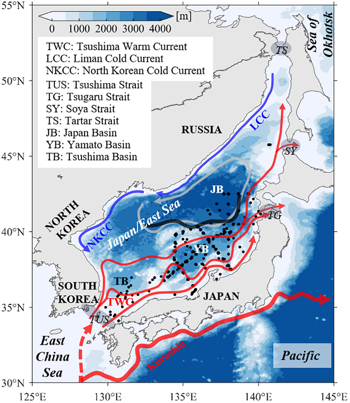
Figure 1 Topography of the JES. Red/blue arrows represent warm/cold currents (Yabe et al., 2021). Black dots indicate the in-situ observation stations of chlorophyll-a concentration, as derived from the WOD18. The dark black line indicates the position of the subpolar front (Zhao et al., 2016; Xi et al., 2022).
Data
The daily SSC data is a Level-4 product providing globally cloud-free estimations during 1998–2019 at a 4-km resolution. The product is published by the Copernicus Marine Environment Monitoring Service (CMEMS), and has merged ocean color observations from multiple sourced satellites (Garnesson et al., 2019). The Level-4 product preserves the information of Level-3 product, and can resolve the SSC variations with time scales longer than intraseasonal (Garnesson et al., 2019; Xu et al., 2021). The in-situ chlorophyll-a concentration measurements at 10 m depth obtained from the World Ocean Database 2018 (WOD18), as shown by the black dots in Figure 1, are used to validate the satellite-derived SSC data in the JES (Boyer et al., 2018). A total of 1172 chlorophyll-a profiles during 1998–2019 was obtained. The satellite-derived SSC data are generally consistent with the in-situ observations, with a high correlation coefficient of 0.79 (p<0.01) (Figure 2). Thus, the satellite-detected SSC data used in this study is reliable for the following research.
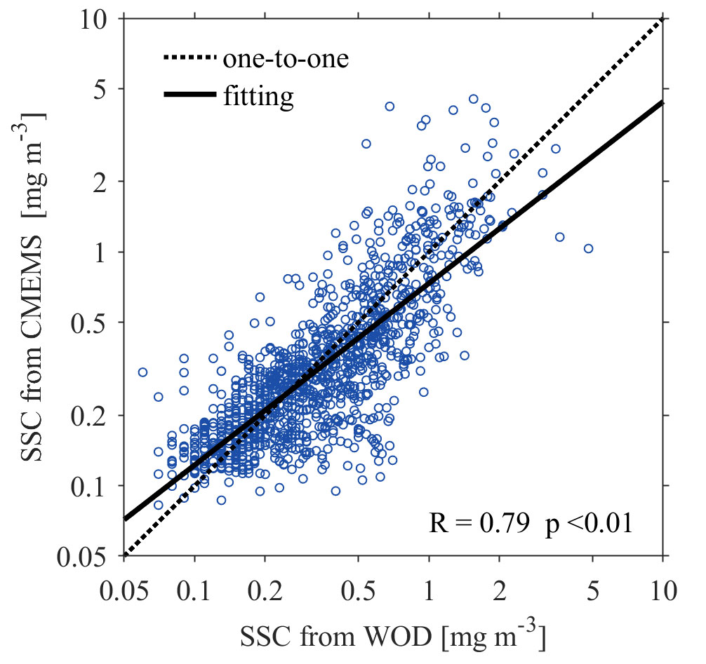
Figure 2 Regression between the in-situ observed chlorophyll-a concentrations from WOD18 (x-axis) and satellite-derived (y-axis) sea surface chlorophyll-a concentrations (SSCs). The dashed line indicates the one-to-one relation.
The photosynthetically active radiation (PAR) and its attenuation coefficient (k) are provided by the European Service for Ocean Colour with a 4-km horizontal resolution and daily interval (Maritorena et al., 2010). Satellite-based SIC data in the Tatar Strait (47°–52°N, 139°–142°E) are obtained from the National Snow and Ice Data Center of the National Oceanic and Atmospheric Administration (Comiso, 2017). The sea surface height (SSH) and sea surface geostrophic current anomalies, with a horizontal resolution of 0.25°×0.25°, are derived from the daily gridded absolute dynamic topography products version 5 and are distributed by the Archiving, Validation, and Interpretation of Satellite Oceanography (Ducet et al., 2000). Daily SST are derived from the CMEMS with a 0.05°×0.05° horizontal resolution (Good et al., 2020). The surface wind vector data are provided by the European Centre for Medium-Range Weather Forecasts ERA5 high-resolution reanalysis project, with a horizontal resolution of 0.25°×0.25° (Hersbach and Dee, 2016). The monthly Niño3.4 and Arctic Oscillation (AO) indices data are collected from the Koninklijk Nederlands Meteorologisch Instituut (KNMI) climate explorer (Trouet and Van Oldenborgh, 2013). In this study, all data described above cover the period from 1 January 1998 to 31 December 2019. Climatological monthly mean temperature, salinity and nutrient profiles are obtained from the World Ocean Atlas 2018 (WOA18) (Garcia et al., 2019). Details for the datasets used in this study are presented in Table 1.
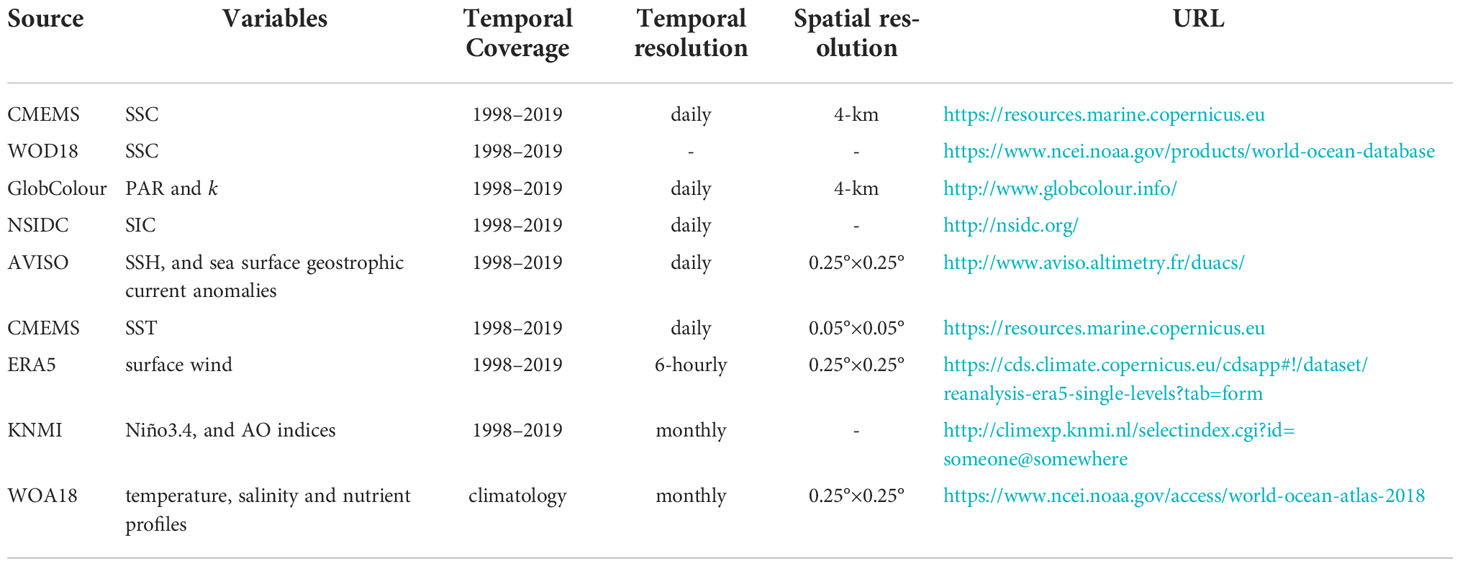
Table 1 Parameters of the datasets used in this study.
Methods
A phytoplankton bloom is defined as a period while the SSC exceeds a certain percentage (20%) of its annual median value over a duration longer than three weeks (spring bloom) or one week (fall bloom), consistent with that used in Maúre et al. (2017). As shown in Figure 3, each grid point has its own threshold SSC value for a bloom. To depict the overall SSC variation characteristics in the JES, we average the SSC over the entire JES. As the definition of blooms on each grid, we identify the blooms for the entire JES with a threshold SSC value calculated from the area-averaged SSC (~0.55 mg m–3). The averaged SSC could also be used to test the EOF results.
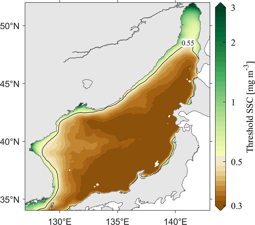
Figure 3 Distribution of threshold SSC for a bloom at each grid in the JES over 1998–2019.
The Ekman pumping velocity is calculated as follows:
where ρ0 = 1.025 × 10³ kg/m3, is the mean sea water density, f is the Coriolis parameter, and τ is the wind stress derived from ERA5 wind field product.
The EKE is calculated as follows:
where u’ and v’ are the sea surface geostrophic current anomalies.
The wind-induced near-inertial energy flux (WNEF) is estimated by a simple slab mixed layer model as follows (Pollard & Millard, 1970):
where Z=u+iv represents the mixed-layer current, H is the area-averaged climatological monthly mean MLD, and τ* is the conjugate of τ. A spectral solution through a two-sided Fourier transform is used here, expressed as the following equation:
Where is the frequency-dependent damping parameter, σ represents the angular frequency, r0 = 0.15f and σc=f/2 (Alford, 2003).
The Brunt Väisälä frequency, N, is used to estimate the vertical stability in the upper 200 m of the ocean as follows:
where g is the gravitational acceleration, ρ is the potential density of sea water, and z is the depth.
The MLD is calculated by defining a temperature threshold of 0.3°C from 10 m, as suggested by Jo et al. (2014). Both N and MLD are calculated from the WOA18 data.
The gradient-based edge detection algorithm is employed to detect SST fronts (Castelao & Wang, 2014; Wang et al., 2021). The monthly frontal probability (FP), which represents the occurrence frequency of SST fronts, is defined as the ratio between the occurrence days of frontal conditions and the total days in the corresponding month.
The critical depth (CRD) is computed as follows:
where I0 is the PAR (E m–2 d–1) and k denotes the attenuation coefficient of PAR. The compensation light intensity Ic is taken as 3.8 E m–2 d–1 (Kim et al., 2000).
Principal component analysis (PCA) is an adaptive data analysis technique to reduce confusing datasets to a lower dimension to increase interpretability, but simultaneously preserves as much ‘variability’ (i.e. statistical information) as possible (Shlens, 2014; Jolliffe and Cadima, 2016; Trombetta et al., 2019). This technique is popular for analysis of atmospheric and oceanic data, and is often referred to as Empirical orthogonal function (EOF) called by Lorenz (1956). Both names are commonly used, and the essence of the two is the same. However, EOF often examines the variability in data through space, which is widely used to extract patterns, while PCA is often used to highlight the relationships between different variables over time (Hannachi et al., 2007; Trombetta et al., 2019). In this study, PCA is used to identify the relevant factors that might influence the seasonal SSC cycle following Trombetta et al. (2019), while EOF is employed to explain the spatiotemporal distribution of SSC in the JES on seasonal and interannual time scales (Legaard and Thomas, 2006; Greene et al., 2019). Prior to the PCA and EOF analysis, the monthly mean SSC data is logarithmically transformed due to its lognormal distribution (Campbell, 1995), as suggested in previous studies (Dandonneau, 1992; Xu et al., 2021).
Results
Seasonal bloom magnitude
The seasonal cycle of the SSC in the JES shows double peaks associated with the bimodal blooms of phytoplankton concentrations in spring and fall, respectively (Figure 4). The JES SSC is at a low level in boreal winter, with values generally smaller than 0.5 mg m–3 (Figures 4A, B). In spring, a bloom occurs around the subpolar front region in March and then extends southward and northward to cover most areas of the JES in April, with SSC values up to 10 mg m–3 (Figures 4C, D). In May, SSC begins to decrease from the southeastern JES (Figure 4E). From June to September, the SSC values are smaller than 0.2 mg m–3 in most regions of the JES except for the Tartar Strait (Figures 4F–I). Fall bloom begins in October, when the SSCs increase slightly over the entire JES, with smaller magnitudes than spring bloom (Figure 4J). The SSCs are higher along the Russian and Korean coasts until December (Figures 4K, L).
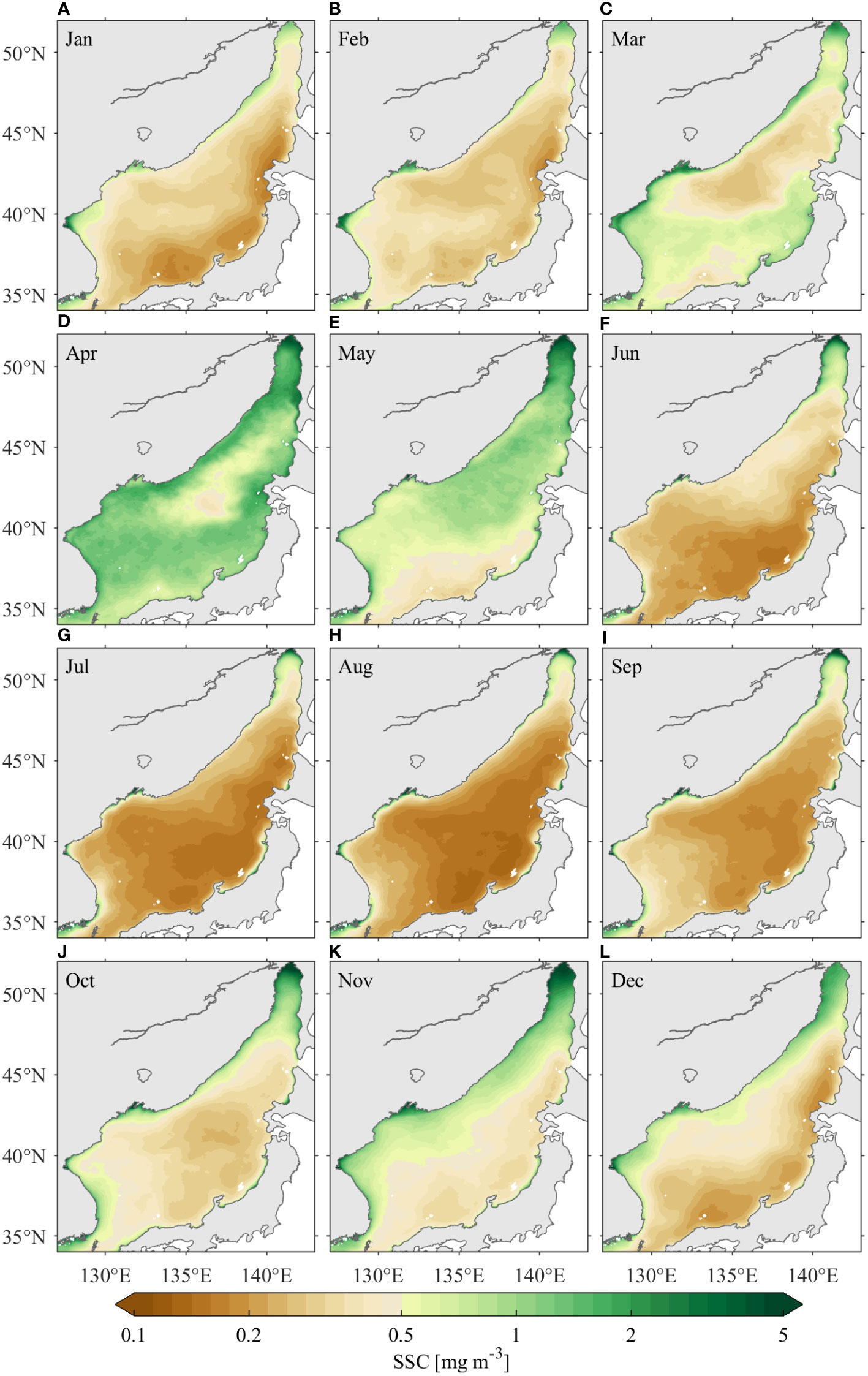
Figure 4 Distribution of climatological monthly mean SSC in the JES over 1998–2019. The subfigures (A–L) are from January to December, respectively.
The seasonal evolution of SSC can be derived by applying EOF analysis on the logarithmic monthly mean SSC (Figure 5). The first three leading EOF modes explain 64.2%, 8.8% and 3.6% of the total variance. The first EOF mode (EOF1) essentially represents the basin-scale seasonal variability in the JES SSC (Figure 5A). The EOF1 is reminiscent of the SSC distribution in April, showing positive values in the entire JES with relatively small magnitudes in the Japan Basin (Figures 5B, C). The seasonal time coefficient of EOF1 coincides with the area-averaged SSC in the JES, showing double peaks of 1.36 ± 0.28 mg m–3 and 0.74 ± 0.07 mg m–3 in April and November, respectively (Figure 5B). During the December–February and June–September periods, the area-averaged SSC is smaller than the threshold criterion, suggesting poor primary production during these stages.
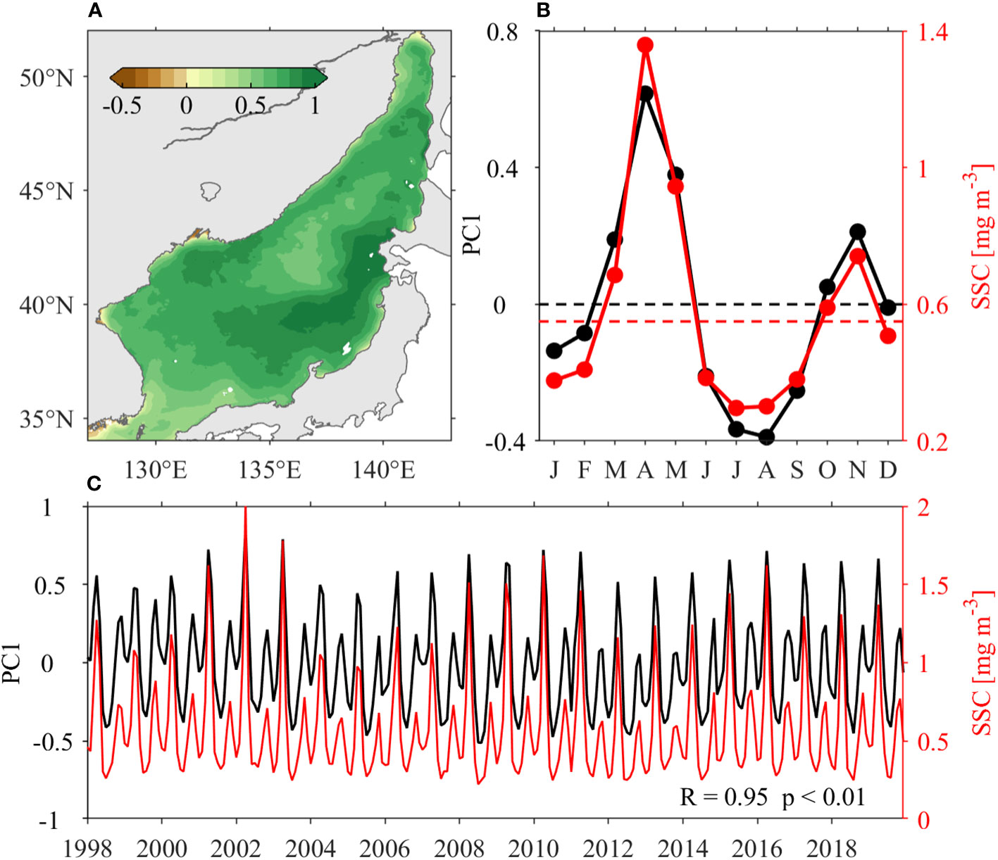
Figure 5 EOF analysis of the logarithmic monthly mean SSC in the JES: (A) spatial pattern of the first EOF mode, (B) climatological and (C) time series (black lines). The red lines in (B) and (C) represent climatological and monthly mean area-averaged SSC values in the JES, respectively. In (B), the black dash line indicates the zero, while the red dashed line indicates the threshold criteria (0.55 mg m–3) of SSC blooms for the entire JES, respectively.
Figure 6 shows the seasonal evolutions of the potential factors accounting for the seasonal variability of SSC in the JES, which have been qualitatively discussed in previous investigations (e.g., Lee et al., 2009; Park et al., 2014; Maúre et al., 2017; Liu et al., 2019; Park et al., 2020). Here, we summarize these factors as four aspects:
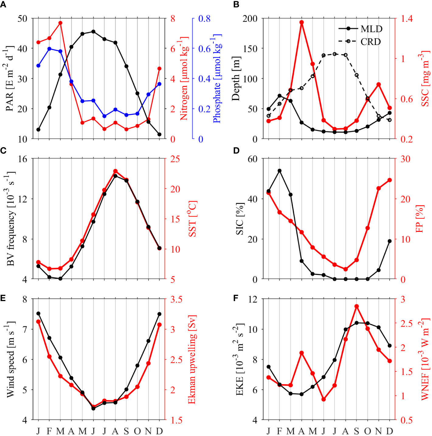
Figure 6 Climatological monthly mean series of area-averaged physical environmental factors and area-averaged SSC: (A) photosynthetically active radiation (PAR, black line), nitrogen (red line) and phosphate (blue line); (B) mixed layer depth (MLD, solid line), critical depth (CRD; dashed line) and SSC (red line); (C) Brunt Väisälä (BV) frequency (black line) and sea surface temperature (SST, red line); (D) sea ice concentration (SIC, black line) and frontal probability (FP, red line); (E) wind speed (black line) and Ekman upwelling transport (red line); (F) eddy kinetic energy (EKE, black line) and wind-induced near-inertial energy flux (WNEF, red line).
(1) PAR and nutrient supply (Figure 6A). In boreal winter, a lower solar altitude angle results in less PAR with an average value of 30.55 E m–2 d–1. In spring or summer, PAR increases due to the raise of solar altitude angle. The upper layers of the JES are rich in nutrients during the boreal winter. Part of these nutrients are stored in sea ice, which serve as an important nutrient supply source when melting in boreal spring (Park et al., 2014). Both nitrogen and phosphate are rapidly consumed during spring blooms, with the nitrogen concentration decreasing from a peak value of 7.68 μmol kg–1 in March to 1.06 μmol kg–1 in May and the phosphate concentration decreasing from a peak value of 0.58 μmol kg–1 in March to 0.25 μmol kg–1 in May. The nutrients supplementation is poor from June to September when SSC is at a low level, and enhance following October.
(2) MLD and CRD (Figure 6B). Due to the annual cycle of PAR, the CRD is deepening from January and becomes equal to the shoaling MLD around February, when SSC becomes to increase rapidly. In autumn, SSC reaches the second peak around November when the deepening MLD the shoaling CRD coincides. However, the initiation timing of spring bloom and fall bloom are later than February and earlier than November, respectively. This time bias might be caused by the value of the Ic, as the temporal variations of Ic, of 6.3 E m–2 d–1 during spring and 1.4 E m–2 d–1 during fall, is not considered in the calculation of CRD (Kim et al., 2000). Thus, the Sverdrup hypothesis (Sverdrup, 1953) is basically applicable to explain the bloom initiation in the JES, indicating that the variations in the JES SSC are mainly governed by the physical environmental conditions.
(3) Stratification (Figure 6C). The JES shows enhanced stratification from March to August due to weakened wind speeds (Figure 6E) and strengthened buoyancy fluxes contributed by both surface warming (Figure 6C) and sea ice melting (Figure 6D). In contrast, destratification occurs from September until the following February. Stratification is basically out of phase with the MLD; this process can be explained by the fact that strong/weak stratification corresponds MLD shoaling/deepening. Since the temporal variations of BV frequency and SST are almost identical, SST is used as the index to quantify stratification in the following analysis.
(4) Ocean dynamics contribute to vertical nutrient-water transport (Figures 6D–F). Ocean dynamics dominate the upper layer nutrients only in boreal summer and fall, when the upper JES is oligotrophic. After October, nutrients increase in accordance with the enhanced upwelling and frontal probability, and under these processes, deeper nutrient-rich waters are entrained to the upper layer. The EKE is larger in the southern JES from August through December, consistent with previous investigation results (Trusenkova, 2014). The WNEF shows larger energy in response to the more frequent typhoons in boreal summer and fall. However, since mesoscale eddies and typhoon-induced near-inertial oscillations generally occur in the southeastern JES, an area that also has strong stratification, it is suggested that only a few typhoons appreciably increase the nutrient supplies in this area (Iwasaki, 2020). Moreover, the high nutrients induced by WNEF are locally distributed along typhoon tracks and thus do not significantly contribute to the area-averaged nutrients over the entire JES. As a result, the monthly averaged nutrients are not efficiently entrained from the deeper layer to the upper layer to nourish the phytoplankton during the June-September period. Nevertheless, the EKE and WNEF remain at relatively high levels until November; therefore, these factors may still contribute to vertical nutrient transport, albeit they are not critical factors.
To identify the dominant and limiting factors affecting the seasonal variability of SSC in the JES, we classify the JES SSC evolution into four stages: the raise stage (January–April) and decline stage (April–July) of spring blooms, and the raise stage (July–November) and decline stage (November–next January) of fall blooms. The relationships between SSC and environmental factors during different stages are examined by PCA analysis (Figure 7). During the raise stage of spring bloom, the SSC is positively correlated with PAR and negatively correlated with wind speed and SIC, suggesting dominant factors inducing spring blooms include increased PAR, weakened winds and sea ice melting. In comparison, oceanic dynamics are not correlated with SSC, as revealed by that they are approximately orthogonal to each other. During the decline stage of spring bloom, the stratification shows a symmetrically opposite relationship with SSC, suggesting that SSC decline is related to enhanced stratification. The PAR is saturated and is thereby orthogonal to SSC, and oceanic dynamics are depressed at this time and thus rarely impact SSC. The coincident directions of SSC and FP occur because subpolar fronts are also undergoing a weakening phase at this time (Park et al., 2007). During the raise stage of fall blooms, SSC is positively correlated with the wind speed, upwelling and oceanic fronts; and negatively correlated with PAR and stratification. These results suggest that destratification, strengthening winds and associated upwelling, and enhanced oceanic fronts, favors an increase in SSC by entraining more nutrient-rich waters to the upper layer. The declining PAR tends to act as a limiting factor for phytoplankton growth when it is reduced to a certain extent. During the decline stage of fall blooms, the winds and associated upwelling tend to enhance the upward transport of nutrient-rich waters to the upper JES. However, limited by decreased PAR and increased sea ice, SSC is still suppressed, resulting in the decay of fall blooms. It is worth noting that the nutrients accumulated during the decline stage of a fall bloom essentially contribute to the following spring bloom.
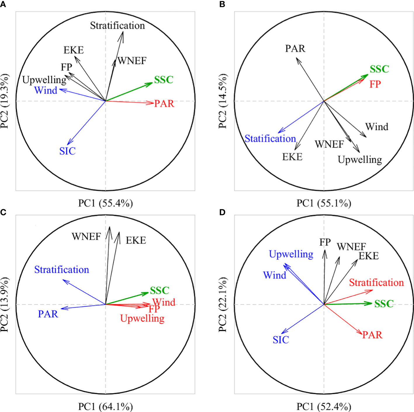
Figure 7 PCA analysis of physical environmental factors (arrows) during different SSC evolution stages: (A) raise (January–April) and (B) decline (April–July) stages of spring blooms; (C) raise (July–November) and (D) decline (November–January) stages of fall blooms. The x- and y-axes represent the first and second principal components (PC1 and PC2), with their variance contributions marked as percentages in brackets of the x- and y-labels respectively. Arrows close to each other denote that the corresponding factors are positively correlated, whereas those are symmetrically opposed to each other suggest they are negatively correlated. Orthogonal arrows mean they are not correlated with each other. The projections of the arrows on the x- and y-axes indicate the extent to which the factors are explained by PC1 and PC2, respectively. The factors positively (negatively) correlated with SSC (green thick arrows) are highlighted with red (blue) arrows.
Interannual bloom magnitude
The spring and fall blooms are attributed to different mechanisms. Therefore, we conduct EOF analyses for the interannual anomalies (remove climatological monthly mean) of logarithmic monthly SSC during spring (March–May) and fall (October–November), respectively. EOF1 accounts for 21.2% and 27.0% of the total variances for the spring and fall blooms, respectively. The large interannual variability of SSC in spring and fall occurs along the JES’s northwestern coast (Figure 8A), and in the deep Japan Basin (Figure 8B), respectively. The positive spring SSC events occur in 2001, 2002, 2009 and 2016, while negative spring SSC events occur in 2005, 2006, 2012 and 2013 (Figure 8C). Positive fall SSC events occur in 1999 and 2015, while negative ones occur in 2008 and 2012 (Figure 8D). Additionally, there is decadal variability in fall blooms, with positive phases during 1998–2002, and 2014–2019, whereas negative phase during 2003–2013.
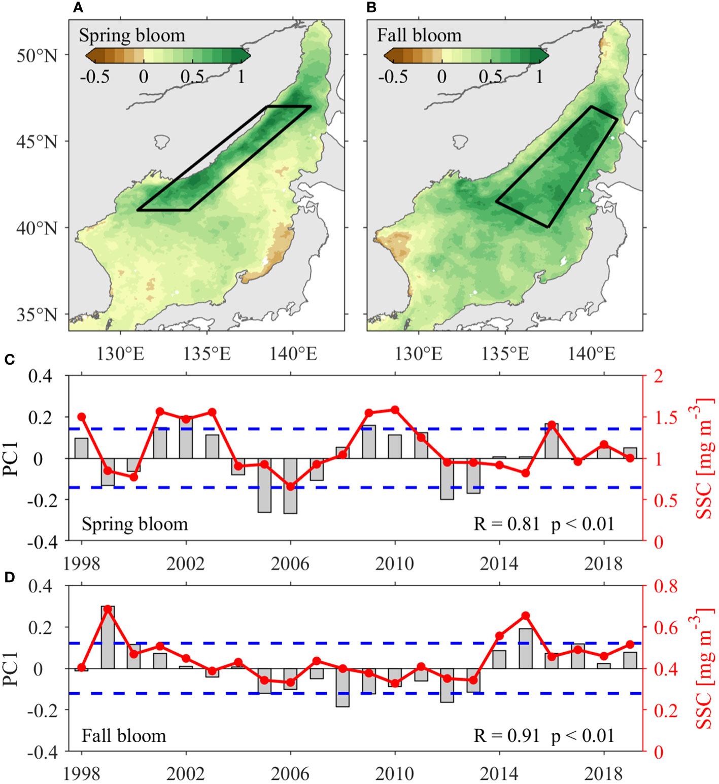
Figure 8 EOF analysis of SSC anomalies in the JES. Spatial patterns of the first EOF mode (EOF1) during (A) spring (March–May) and (B) fall (October–November). The annual time series of EOF1 (PC1, grey bars) with standard deviation (blue dash lines), and area-averaged SSC anomalies (red lines) during (C) spring and (D) fall. The areas averaged SSC anomalies for (C) and (D) are marked with black boxes in (A) and (B), respectively.
The interannual variability of JES SSC is positively correlated with PAR, with correlation coefficient (R) of 0.37 at a confidence level of p< 0.1 in spring and of R = 0.12, p > 0.1 in fall (Figures 9A, C). For stratification anomalies, the correlations are R = 0.55, p< 0.01 in spring and R = –0.44, p< 0.05 in fall (Figures 9B, D). These correlations suggest that PAR positively contributes to the interannual SSC variability in the JES in spring. Meanwhile, strong stratification favors positive SSC anomalies in spring, as explained by the critical depth hypothesis. In contrast, PAR anomalies are not significantly correlated with SSC anomalies in fall, whereas stratification shows a significant negative correlation, suggesting that stronger stratification leads to smaller SSCs by inhibiting the upward transport of nutrient-rich waters to the mixed layer. For spring bloom, the interannual variability of JES SSC shows weak positive correlation with AO (R = 0.38, p<0.1) and ENSO (R = 0.26, p > 0.1). These correlations suggest that the spring bloom magnitude would increase during positive AO and El Niño events, corroborating with the previous study (Park et al., 2022). On the contrary, both the ENSO and AO are not significantly correlated with the interannual variability of fall bloom magnitude, with correlation coefficients of 0.05 and –0.04, respectively, below the 90% confidence level.
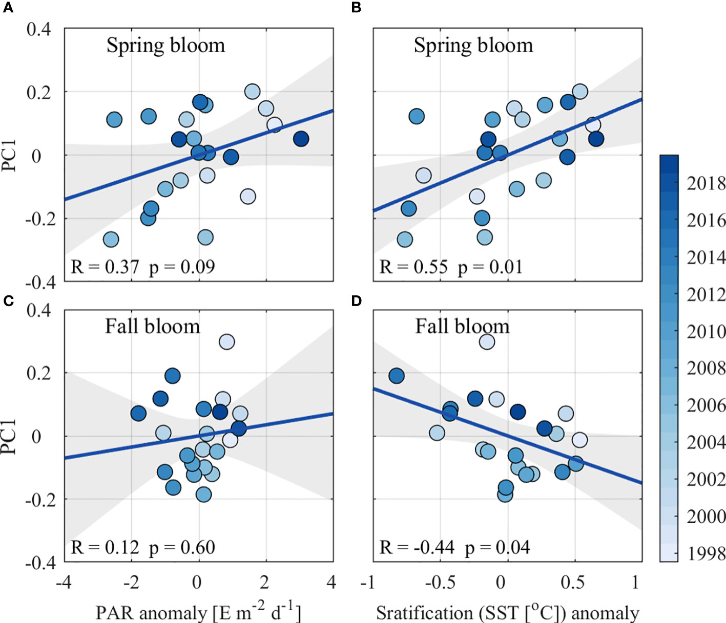
Figure 9 Scatterplots (colored dots) and linear fitting (blue lines) between PAR anomalies and PC1 in (A) spring and (C) fall and between stratification anomalies and PC1 in (B) spring and (D) fall. The gray shading indicates the 95% two‐sided confidence bounds.
Bloom timing
Spring bloom initiates in the southern and southeastern JES in February–March and in the northwestern JES in April (Figure 10A), in agreement with previous investigations (e.g., Kim et al., 2000; Yamada et al., 2004; Park et al., 2020). Fall blooms initiates in the Tsushima Basin and along the JES coasts from September to early October and in the central basin of the JES from late October to early November (Figure 10B). Spring blooms are terminated generally in the southwestern JES on 11 April ± 9 days and subsequently in the northeastern JES on 29 May ± 9 days (Figure 10C). Fall blooms generally terminate on 29 November ± 12 as a result of the rapidly decreasing PAR beginning in late November (Figure 10D).
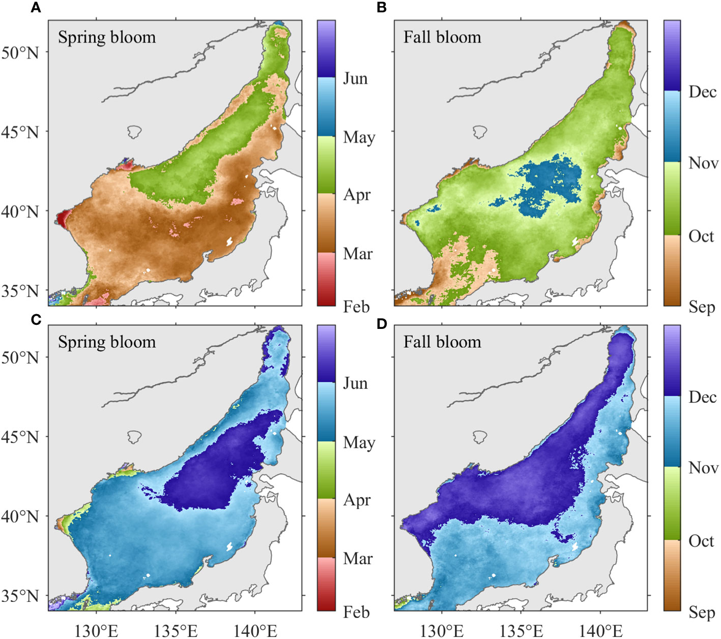
Figure 10 The climatological distributions of the initiation timing of (A) spring and (B) fall blooms; and the termination timing of (C) spring and (D) fall blooms.
Figure 11 shows the initiation and termination timing of spring blooms along the JES’s northwestern coast during 1998–2019. Spring blooms were initiated earlier in 2002, 2010, 2011 and 2014 and later in 1999, 2005, 2006, and 2013; and were terminated earlier in 2002, 2003, 2010 and 2011 and later in 1999, 2000, 2003, and 2006, identified by a threshold value of one standard deviation beyond the climatological mean initiation/termination timing (Figure 11A). The interannual variability in initiation timing is jointly correlated by PAR, stratification, and sea ice melting, i.e., higher PAR, stronger stratification, and earlier sea ice melting are favorable for earlier spring blooms (Figures 11B–D). The termination and initiation timing of spring blooms are significantly correlated, with a correlation coefficient of 0.74 (p<0.01). Additionally, the initiation/termination timings show trends of occurring earlier by 0.37/0.45 days per year during 1998–2019, coinciding with the increasing trends in PAR and stratification identified in March and April.
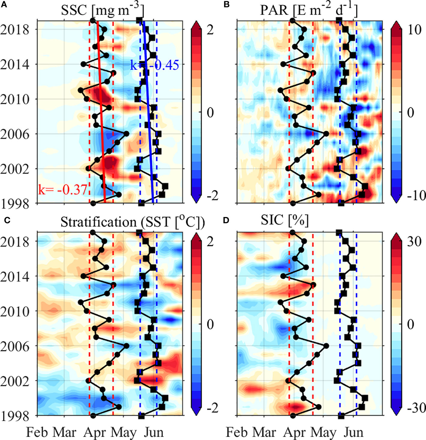
Figure 11 (A) SSC, (B) PAR, (C) stratification, and (D) SIC anomalies (shadings) averaged along the JES’s northwestern coast (marked by the black box in Figure 8A) from 1998 to 2019. The spring bloom initiation and termination timing are represented by solid dots and square lines, with the solid red/blue lines indicating the linear trends, and the dashed red/blue lines indicating the one standard deviation beyond the climatological mean initiation/termination timing, respectively.
In the deep Japan Basin, fall blooms were initiated earlier in 1999, 2015, and 2019, in accordance with strong winds and weak stratification; and were initiated later in 2003, 2006, 2008 and 2010, when weak winds and strong stratification occurred. The fall blooms were terminated early in 2011, 2012, 2017 and 2018 and late in 1998, 1999, 2000, and 2015 (Figure 12A). In comparison to the significant positive correlation observed between the termination and initiation timing of spring blooms, the corresponding correlation coefficient of fall blooms is only 0.21 (p>0.1). In addition, the initiation/termination timing show trends of occurring earlier by 0.49/1.28 days per year during 1998–2019, which may be related to the weakened stratification (caused by the intensified wind speeds)/weakened wind speeds during the fall bloom development/decay periods, respectively (Figures 12B, C).
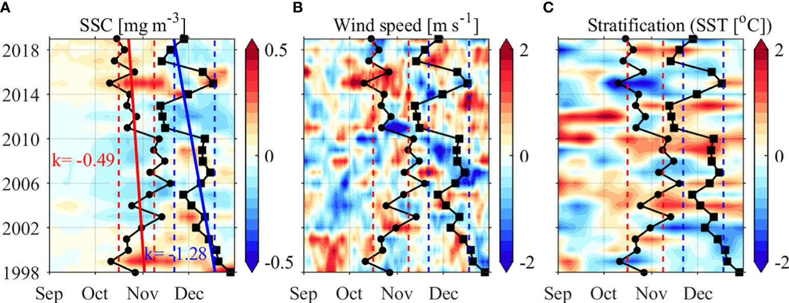
Figure 12 (A) SSC, (B) PAR, and (C) stratification anomalies (shadings) averaged in the deep Japan Basin (marked by the black box in Figure 8B) from 1998 to 2019. The fall bloom initiation/termination timing are represented by solid dots/square lines, with the solid red/blue lines indicating the linear trends, and the dashed red/blue lines indicating the one standard deviation beyond the climatological mean initiation/termination timing, respectively.
As shown in Figure 13A, for spring bloom along the JES’s northwestern coast, in case the bloom occurs earlier, its duration tends to be longer (R = -0.72, p< 0.01). The SSC anomalies from March to May are negatively correlate with initiation (R = -0.50, p< 0.05) and termination (R = -0.55, p< 0.01) timing anomalies, but not statistically correlated with duration anomalies (R = 0.16, p > 0.1). In addition, the spring blooms along the JES’s northwestern coast would occur earlier (R = -0.47, p< 0.05) and be more prolonged (R = 0.37, p< 0.1) during positive AO, and would terminate earlier during El Niño events (R = -0.42, p< 0.1). For fall bloom in the deep Japan Basin, duration anomalies are mainly affected by the initiation timing anomalies with a negative correlation coefficient of -0.57 above 99% confidence level (Figure 13B). In addition, on interannual time scale, the bloom magnitude is negatively correlated with the initiation timing with a value of -0.73 (p<0.01), and positively correlated with bloom duration with a value of 0.78 (p<0.01). Furthermore, neither the ENSO nor the AO show significant correlations with the interannual variability of fall bloom timing.
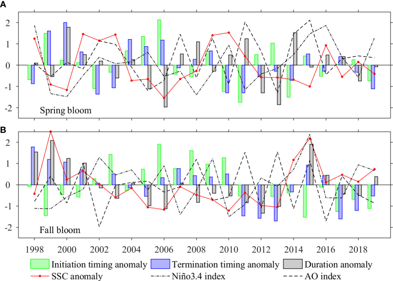
Figure 13 Time series of initiation timing anomalies (green bars), termination timing anomalies (blue bars), duration anomalies (gray bars), area averaged SSC anomalies (red lines), Niño 3.4 index (black dot-dash lines) and AO index (black dashed lines) for (A) spring, and (B) fall blooms. The averaged areas are marked by black box in Figures 8A, B for spring and fall blooms, respectively. The time series of all variables are normalized, i.e., divided by their corresponding standard deviations (STD).
Discussion
The JES is known as a mid-latitude “Miniature Ocean” in which multiscale oceanic dynamical processes (e.g., cross-basin warm and cold currents, upwelling, oceanic fronts, mesoscale eddies, and near-inertial oscillations) and sea ice occur. The marine ecosystems of the JES are influenced by these complicated processes. The phytoplankton concentrations can be evidenced by the SSC variability. Previous investigations have revealed bimodal phytoplankton concentrations blooms occurring in spring and fall. In this study, based on a newly released high-resolution satellite-derived SSC product, we revisit the spring and fall phytoplankton blooms and their driven factors during the raise and decline stages. In addition to the previously MLD-CRD theory, here we emphasize that different factors tend to play dominant role during the raise and decline stages of the spring and fall blooms. The increased PAR, weakened winds and sea ice melting are dominant for the spring bloom until the nutrients are exhausted and with no supplementary because of enhanced stratification, and thus terminates the spring bloom. The intensified wind and oceanic dynamical processes lead to destratification, which then triggers the fall bloom by entraining nutrient-rich water to the upper layer. The fall bloom is terminated by the rapidly declining of PAR, which acts as a limiting factor for phytoplankton growth when it is reduced to a certain extent.
It is interesting that the interannual JES SSC are not statistically significant correlated with the ENSO. However, existing studies have suggested that the JES is indeed influenced by ENSO on interannual time scales (e.g., Wang et al., 2000; Wang and Chan, 2002; Son et al., 2016; He et al., 2017; Cheon, 2020). Furthermore, case studies suggest the El Niño events could induce JES SSC anomaly in terms of bloom timing (Yamada et al., 2004; Yoo and Kim, 2004). Hence, we conducted composite analyses by comparing the JES SSC anomaly and initiation timing anomaly in El Niño and La Niña years, respectively (Figure 14). A total of three El Niño events (2002–2003, 2009–2010 and 2015–2016) and six La Niña events (1998–1999, 1999–2000, 2007–2008, 2010–2011, 2011–2012 and 2017–2018) are considered for the composite analyses, with the weak events (the absolute Niño 3.4 index below 1.0°C) being excluded. As shown in Figures 14A–C, there are high/low SSC anomaly in El Niño/La Niña years, with differences above the 95% confidence level along the northwestern coast of the JES, coincide with the EOF pattern (see Figure 8A). The coincidence patterns between the composite and EOF analyses suggest the interannual variability of the JES SSC in spring should closely associate with the ENSO events. Meanwhile, earlier spring blooms are found in El Niño years, which is in agreement with Yamada et al. (2004). In comparison, the composite analyses of JES SSC in fall show different pattern from the EOF analysis, albeit there are significant differences of SSC anomalies in the northwestern of the JES (Figures 14G–I).
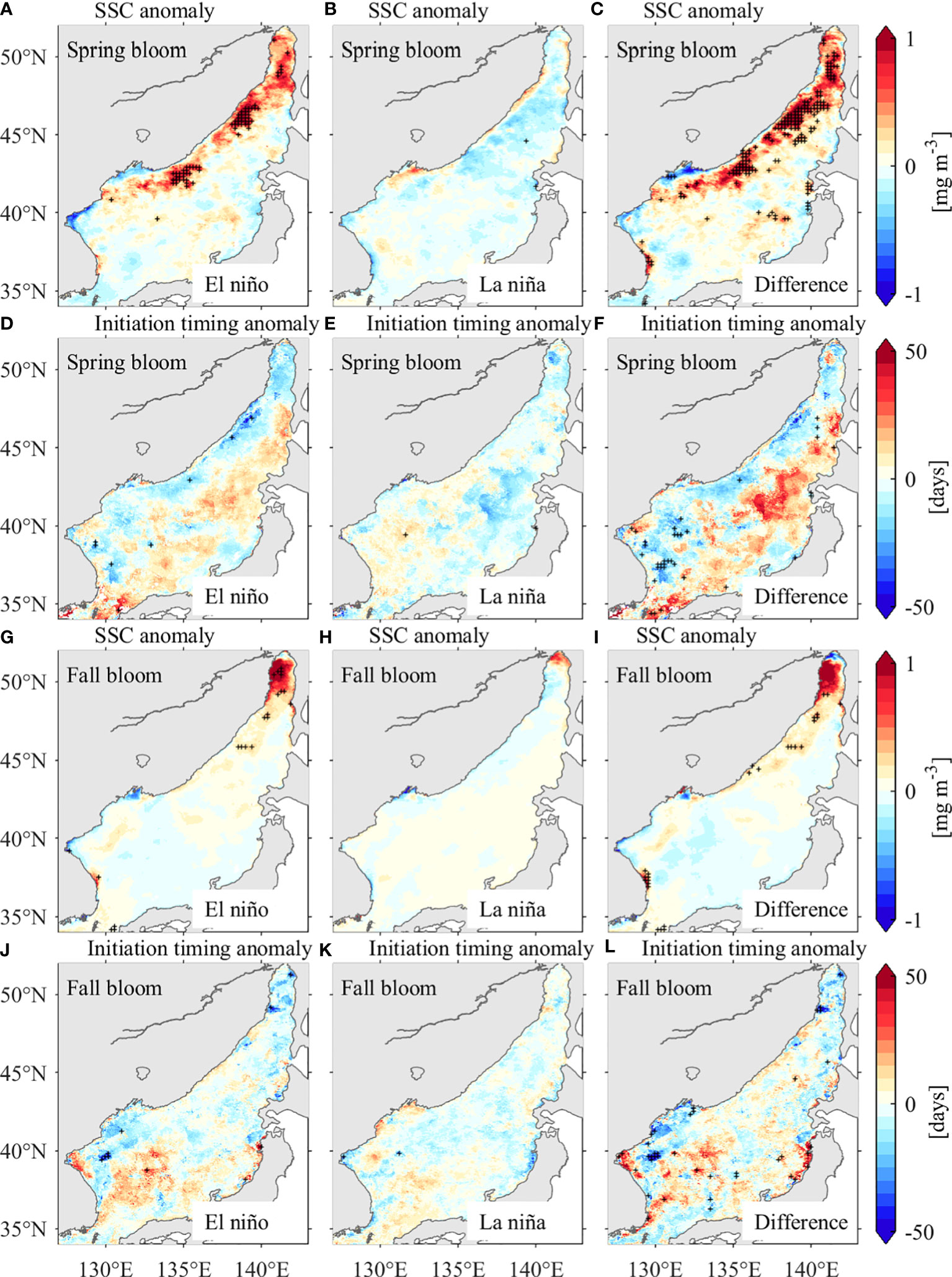
Figure 14 Spring bloom magnitude anomalies during El Niño events (A) and La Niña events (B), and their difference (C). (D–F) are same as (A–C), but for the spring bloom initiation timing anomalies. (G–L) are same as (A–F),but for fall blooms. Areas with plus sighs indicate that the difference is statistically significant at the 95% confidence level. El Niño events: 2002–2003, 2009–2010 and 2015–2016. La Niña events: 1998–1999, 1999–2000, 2007–2008, 2010–2011, 2011–2012 and 2017–2018.
Figure 15 shows the time series of composed SSC and physical environmental factors anomalies along the northwestern coast of the JES in El Niño/La Niña years. There are high SSC anomalies in the following spring of El Niño peak (Figure 15A). The positive SSC anomalies of spring blooms in El Niño years can be explained by more sea ice in the previous winter, weaker wind speed during the raise stage and stronger stratification throughout the spring bloom period (Figures 15C, D, F), which lead to the spring blooms start slightly earlier. Similar composite analysis has been done for fall blooms, which does not show out of phase relationship for JES SSC anomalies between El Niño and La Niña years (Figures omitted). This can be explained by the fact that ENSO event-induced anomalies somehow result in contradictory SSC responses in the JES. For instance, higher SSCs and longer bloom durations are expected, as active typhoons benefit the vertical transport of nutrient-rich waters during El Niño years (Goh and Chan, 2010). However, at the same time, the warmer background states that occur during the summer-fall seasons in the JES act to inhibit SSC increases and thus cancel out the role of typhoons (Cheon, 2020). The insensitive response of JES SSC in fall is in agreement with previously investigation (Park et al., 2020).
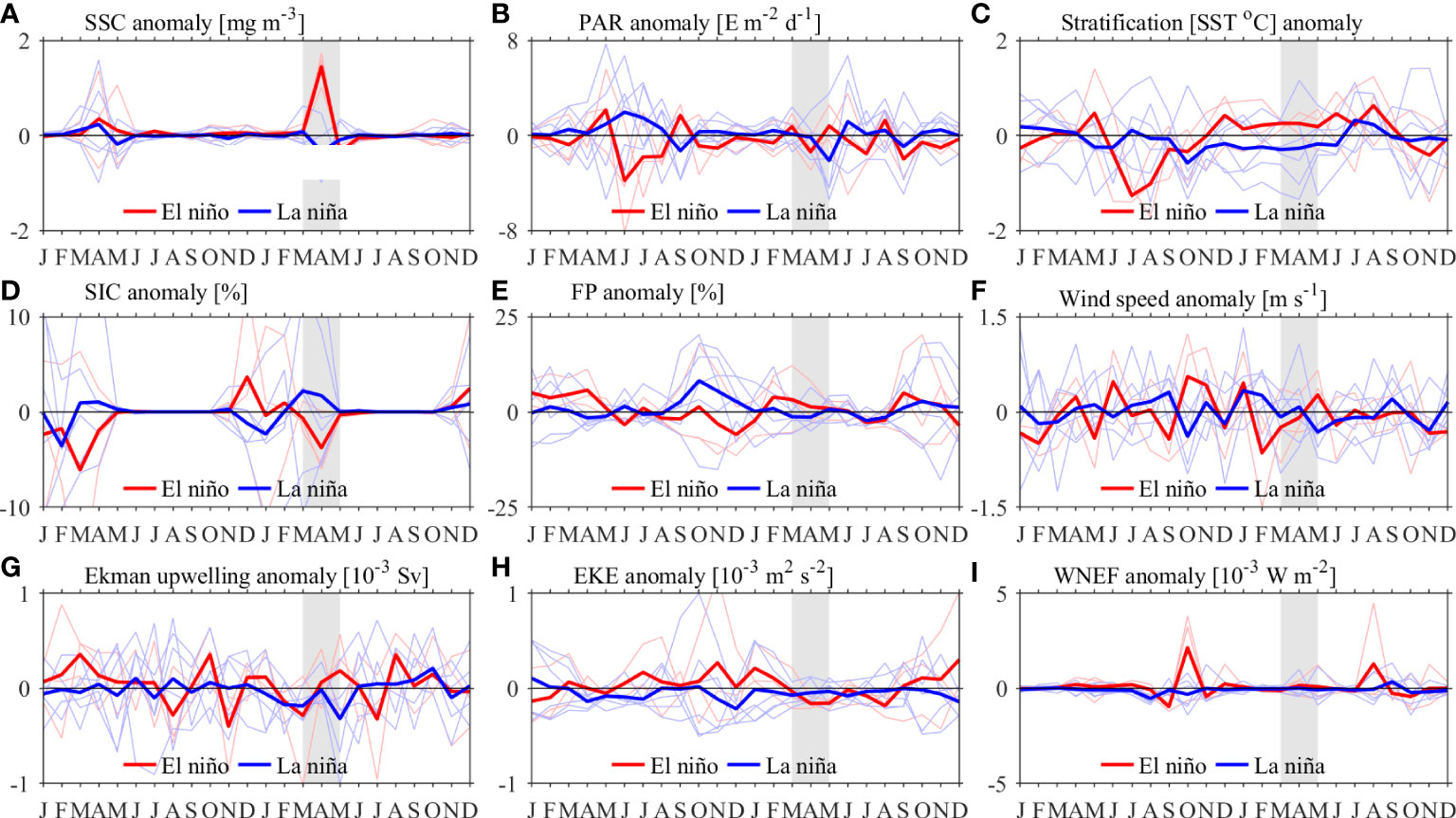
Figure 15 Time series of SSC anomalies and physical environmental factors anomalies averaged along the JES’s northwestern coast (marked by the black box in Figure 8A) during El Niño events (red lines) and La Niña events (blue lines), while the thick lines represent the average of the corresponding time series: (A) SSC; (B) PAR; (C) Stratification; (D) SIC; (E) FP; (F) wind speed; (G) Ekman upwelling transport; (H) EKE and (I) WNEF. Gray shaded areas indicate spring bloom period following El Niño peak. El Niño events: 2002–2003, 2009–2010 and 2015–2016. La Niña events: 1998–1999, 1999–2000, 2007–2008, 2010–2011, 2011–2012 and 2017–2018.
The bloom magnitude anomaly is not statistically correlated with bloom duration anomaly in spring at interannual time scale. This lack of correlation can be attributed to different control factors affecting the durations and magnitudes of spring blooms. There is adequate light in the entire JES during the spring bloom period, while strong stratification prevents the upward transport of deep, nutrient-rich waters to supply the upper layer. Therefore, the bloom duration is mainly controlled by the consumption rate of the accumulated nutrients in the upper layer (e.g., Bouman et al., 2011; Jo et al., 2014; Park et al., 2020). SSC is a phytoplankton biomass indicator that is related to the amount of accumulated nutrients (Maúre et al., 2017). Both the phytoplankton biomass and the bloom duration are positively correlated with the accumulated nutrients. However, more phytoplankton biomass leads to faster nutrient consumption. Thus, this relation tends to result in a negative correlation between the durations of and SSC anomalies associated with spring blooms. As a result, no significant correlation is found between the spring bloom durations and SSC anomalies.
In comparison, the interannual variability of fall bloom magnitude is significantly correlated with the interannual variability its duration. Nutrients are limited during the fall bloom period. Therefore, the growth of phytoplankton biomass depends on the nutrients supplied by the vertical transport of deep waters through dynamic oceanic processes (e.g., Yamada et al., 2004; Andreev, 2014; Jo et al., 2014). Moreover, these nutrients are consumed immediately after being transported to the upper layer, and thus, the consumption rate of the nutrients can be ignored. Persistent and active oceanic dynamic processes tend to transport more nutrient-rich waters to the upper layer, favoring both increased SSCs and prolonged fall bloom durations.
Beyond of above discussion, some issues remain unclear, including but not limited to (1) obtaining a quantitative assessment of the driving factors that account for JES SSC variabilities; (2) the relation between JES SSCs and climate change; and (3) the JES SSC variabilities induced by changes in the phytoplankton community structure and the interactions between grazers and phytoplankton. Especially, the complex predator-prey interactions are crucial to the temporal changes in phytoplankton concentrations (Behrenfeld, 2010; Behrenfeld and Boss, 2017). Thus, these pending issues must be further investigated through interdisciplinary collaboration.
Summary
In this study, we investigate the spring and fall phytoplankton blooms and their interannual variability by employing high-resolution satellite remote sensing products. The new findings are summarized as follows.
(1) JES SSC is characterized by bimodal blooms in spring and fall. Different physical environmental factors are responsible for the JES SSC evolution during the raise and decline stages of the spring and fall blooms. Increased PAR, weakened winds and melting sea ice are the favorable factors for the initiation of spring blooms. Enhanced stratification, which inhibits the upward transport of nutrient-rich waters to the upper layer to compensate for the rapid consumption of nutrients, is the controlling factor inducing the termination of spring blooms. Destratification and active oceanic dynamic processes are favorable factors for fall blooms because they transport nutrient-rich waters to the upper layer. Declining PAR tends to serve as a limiting factor for phytoplankton growth when it is reduced to a certain extent, thereby resulting in the termination of fall blooms.
(2) The interannual variability in the JES SSC consists of spring and fall components, which occur along the JES’s northwestern coast and in the deep JES basin, respectively. Stronger PAR and stratification favor positive SSC anomalies of spring bloom, whereas weaker stratification favors positive SSC anomalies of fall bloom. It is found that positive SSC anomalies along the northwestern coast of the JES tend to occur in the following spring of El Niño peak, as a result of more sea ice in the previous winter, weaker wind speed during the raise stage and stronger stratification throughout the spring bloom period. No significant relationship has been found between the fall bloom and ENSO.
(3) Spring blooms are initiated in the southern and southeastern JES in February–March and in the northwestern JES in April, with climatological mean initiation dates of 13 March ± 9 and 8 April ± 10 days, respectively. Fall blooms are initiated in the Tsushima Basin and along the JES coasts from September to early October and in the central basin of the JES from late October to early November, with climatological mean initiation dates of 6 October ± 12 and 27 October ± 6 days, respectively. Spring blooms are terminated in the southwestern JES on 11 April ± 9 days and, subsequently, in the northeastern JES on 29 May ± 9 days. Fall blooms are generally terminated on 29 November ± 12. For spring blooms, the interannual variability in the bloom duration are not statistically correlated with the that in bloom magnitude because these characteristics are dominated by different factors, i.e., PAR and wind speed affect the initiation timing, while accumulated nutrients affect the bloom magnitude. For fall blooms, the interannual variabilities in the bloom duration and that in bloom magnitude are significantly correlated with each other with a correlation coefficient of 0.78, which are both dominated by oceanic dynamical processes. The initiation/termination timing of spring blooms has shifted earlier by 0.37/0.45 days annually along the JES’s northwestern coast; the counterpart of fall blooms has shifted 0.49/1.28 days earlier annually in the deep Japan Basin.
Data availability statement
The original contributions presented in the study are included in the article/supplementary material. Further inquiries can be directed to the corresponding author.
Author contributions
DW: Data curation, Methodology, Visualization, Writing – original draft. GHF: Writing – review & editing, Supervision. SJ: Methodology, Writing – original draft. QX, GW, and YW: Writing – review & editing. ZW: Writing – review & editing, Funding acquisition. TX: Writing – review & editing, Resources, Funding acquisition. All authors contributed to the article and approved the submitted version.
Funding
This study is jointly supported by the National Key Research and Development Program of China (Grant No. 2020YFA0608800), and the National Natural Science Foundation of China (Grant No. 41821004). This work got the data service support from the Marine Environment Data Service System which supported by the National Key Research and Development Program of China (2019YFC1408405).
Conflict of interest
The authors declare that the research was conducted in the absence of any commercial or financial relationships that could be construed as a potential conflict of interest.
Publisher’s note
All claims expressed in this article are solely those of the authors and do not necessarily represent those of their affiliated organizations, or those of the publisher, the editors and the reviewers. Any product that may be evaluated in this article, or claim that may be made by its manufacturer, is not guaranteed or endorsed by the publisher.
References
Alford M. H. (2003). Improved global maps and 54-year history of wind-work on ocean inertial motions. Geophys. Res. Lett. 30 (8), 1424. doi: 10.1029/2002GL016614
Andreev A. G. (2014). Interannual variations of sea water parameters and chlorophyll a concentration in the Japan Sea in autumn. Russian Meteorol. Hydrol. 39 (8), 542–549. doi: 10.3103/S1068373914080068
Banse K. (1977). Determining the carbon-to-chlorophyll ratio of natural phytoplankton. Mar. Biol. 41, 199–212. doi: 10.1007/BF00394907
Behrenfeld M. J. (2010). Abandoning sverdrup’s critical depth hypothesis on phytoplankton blooms. Ecology 91 (4), 977–989. doi: 10.1890/09-1207.1
Behrenfeld M. J., Boss E. S. (2017). Student’s tutorial on bloom hypotheses in the context of phytoplankton annual cycles. Global Change Biol. 24 (1), 55–77. doi: 10.1111/gcb.13858
Bouman H. A., Ulloa O., Barlow R., Li W. K., Platt T., Zwirglmaier K., et al. (2011). Water-column stratification governs the community structure of subtropical marine picophytoplankton. Environ. Microbiol. Rep. 3 (4), 473–482. doi: 10.1111/j.1758-2229.2011.00241.x
Boyer T. P., Baranova O. K., Coleman C., Garcia H. E., Grodsky A., Locarnini R. A., et al. (2018). World ocean database 2018. Ed. Mishonov A. V., 87, NOAA Atlas NESDIS. Available at: https://www.ncei.noaa.gov/sites/default/files/2020-04/wod_intro_0.pdf.
Brody S. R., Lozier M. S. (2014). Changes in dominant mixing length scales as a driver of subpolar phytoplankton bloom initiation in the North Atlantic. Geophysical Research Letters 41, 3197–3203. doi: 10.1002/2014GL059707
Campbell J. W. (1995). The lognormal distribution as a model for bio-optical variability in the sea. J. Geophys. Res. 100 (C7), 13237–13254. doi: 10.1029/95JC00458
Castelao R. M., Wang Y. (2014). Wind-driven variability in sea surface temperature front distribution in the California current system. J. Geophys. Res. Oceans 119 (3), 1861–1875. doi: 10.1002/2013JC009531
Cheon W. G. (2020). The Summer/Fall variability of the southern East/Japan Sea in the ENSO period. Ocean Sci. J. 55, 341–352. doi: 10.1007/s12601-020-0027-5
Chiswell S. M., Bradford-Grieve J., Hadfield M. G., Kennan S. C. (2013). Climatology of surface chlorophyll a, autumn-winter and spring blooms in the southwest pacific ocean. J. Geophys. Res. Oceans 118, 1003–1018. doi: 10.1002/jgrc.20088
Comiso J. C. (2017). Bootstrap Sea Ice Concentrations from Nimbus-7 SMMR and DMSP SSM/ISSMIS, Version 3 Boulder. Colorado USA: NASA National Snow and Ice Data Center Distributed Active Archive Center. doi: 10.5067/7Q8HCCWS4I0R
Dandonneau Y. (1992). Surface chlorophyll concentration in the tropical pacific ocean: an analysis of data collected by merchant ships from 1978 to 1989. J. Geophys. Res. 97 (C3), 3581–3591. doi: 10.1029/91JC02848
Ducet N., Le, Traon P. Y., Reverdin G. (2000). Global high-resolution mapping of ocean circulation from TOPEX/Poseidon and ERS-1 and-2. J. Geophys. Res. Oceans 105 (C8), 19477–19498. doi: 10.1029/2000JC900063
Garcia H. E., Boyer T. P., Baranova O. K., Locarnini R. A., Mishonov A. V., Grodsky A., et al. (2019) World ocean atlas 2018: Product documentation. Ed. Mishonov A.. Available at: https://www.ncei.noaa.gov/sites/default/files/2022-06/woa18documentation.pdf.
Garnesson P., Mangin A., D'Andon O. F., Demaria J., Bretagnon M. (2019). The CMEMS GlobColour chlorophyll a product based on satellite observation: multi-sensor merging and flagging strategies. Ocean Sci. 15, 819–830. doi: 10.5194/os-15-819-2019
Goh A. Z., Chan J. C. L. (2010). Variations and prediction of the annual number of tropical cyclones affecting Korea and Japan. International Journal of Climatology 32 (2), 178–189. doi: 10.1002/joc.2258
Good S., Fiedler E., Mao C., Martin M. J., Maycock A., Reid R., et al. (2020). The current configuration of the OSTIA system for operational production of foundation Sea surface temperature and ice concentration analyses. Remote Sens. 12, 720. doi: 10.3390/rs12040720
Greene C. A., Thirumalai K., Kearney K. A., Delgado J. M., Schwanghart W., Wolfenbarger N. S., et al. (2019). The climate data toolbox for MATLAB. Geochemistry, Geophysics, Geosystems 20, 3774–3781. doi: 10.1029/2019GC008392
Hannachi A., Jolliffe I. T., Stephenson D. B. (2007). Empirical orthogonal functions and related techniques in atmospheric science: A review. Int. J. Climatol. 27 (9), 1119–1152. doi: 10.1002/joc.1499
Hays G., Richardson A., Robinson C. (2005). Climate change and marine plankton. Trends Ecol. Evol. 20 (6), 337–344. doi: 10.1016/j.tree.2005.03.004
He S., Gao Y., Li F., Wang H., He Y. (2017). Impact of Arctic oscillation on the East Asian climate: A review. Earth-Sci. Rev. 164, 48–62. doi: 10.1016/j.earscirev.2016.10.014
Ichiye T. (1984). Some problems of circulation and hydrography of the Japan Sea and the tsushima current. Elsevier Oceanogr. Ser. 39, 15–54. doi: 10.1016/S0422-9894(08)70289-7
Ishizaka J., Yamada K. (2019). “Phytoplankton and primary production in the Japan Sea,” in Remote sensing of the Asian seas. Eds. Barale V., Gade M. (Cham: Springer), 177–189. doi: 10.1007/978-3-319-94067-0_9
Ivanova E. V., Ivanov V. V. (2012). The amur river runoff formation in the amur liman. Russian Meteorol. Hydrol. 37, 631–639. doi: 10.3103/S1068373912090075
Iwasaki S. (2020). Daily variation of chlorophyll-A concentration increased by typhoon activity. Remote Sensing 12 (8), 1259. doi: 10.3390/rs12081259
Ji C., Zhang Y., Cheng Q., Tsou J. Y. (2021). Investigating ocean surface responses to typhoons using reconstructed satellite data. Int. J. Appl. Earth Obs. Geoinfo. 103, 102474. doi: 10.1016/j.jag.2021.102474
Jolliffe I. T., Cadima J. (2016). Principal component analysis: a review and recent developments. Philos. Trans. R. Soc. A 374, 20150202. doi: 10.1098/rsta.2015.0202
Jo C. O., Park S., Kim Y. H., Park K., Park J. J., Park M., et al. (2014). Spatial distribution of seasonality of SeaWiFS chlorophyll-a concentrations in the East/Japan Sea. J. Mar. Syst. 139, 288–298. doi: 10.1016/j.jmarsys.2014.07.004
Kim K., Chang K., Kang D., Kim Y. H., Lee J. (2008). Review of recent findings on the water masses and circulation in the East Sea(Sea of Japan). J. Oceanogr. 64, 721–735. doi: 10.1007/s10872-008-0061-x
Kim S., Saitoh S., Ishizaka J., Isoda Y., Kishino M. (2000). Temporal and spatial variability of phytoplankton pigment concentrations in the Japan Sea derived from CZCS images. J. Oceanogr. 56, 527–538. doi: 10.1023/A:1011148910779
Kim H., Yoo S., Oh I. S. (2007). Relationship between phytoplankton bloom and wind stress in the sub-polar frontal area of the Japan/East Sea. J. Mar. Syst. 67, 205–216. doi: 10.1016/j.jmarsys.2006.05.016
Kodama T., Wagawa T., Ohshimo S., Morimoto H., Iguchi N., Fukudome K., et al. (2018). Improvement in recruitment of Japanese sardine with delays of the spring phytoplankton bloom in the Sea of Japan. Fish. Oceanogr. 27, 289–301. doi: 10.1111/fog.12252
Lee J., Kang D., Kim I., Rho T., Lee T., Kang C., et al. (2009). Spatial and temporal variability in the pelagic ecosystem of the East Sea (Sea of japan): A review. J. Mar. Syst. 78 (2), 288–300. doi: 10.1016/j.jmarsys.2009.02.013
Lee D. K., Niiler P. (2010). Eddies in the southwestern East/Japan Sea. Deep-Sea Res. I 57 (10), 1233–1242. doi: 10.1016/j.dsr.2010.06.002
Lee S., Yoo S., Son Y. B. (2015). Variability of chlorophyll-a bloom timing associated with physical forcing in the East Sea/Sea of Japan, (1998–2014). 167.
Legaard K. R., Thomas A. C. (2006). Spatial patterns in seasonal and interannual variability of chlorophyll and sea surface temperature in the California current. J. Geophys. Res. 111, C06032. doi: 10.1029/2005JC003282
Liu Y., Tang D., Evgeny M. (2019). Chlorophyll concentration response to the typhoon wind-pump induced upper ocean processes considering air-Sea heat exchange. Remote Sens. 11, 1825. doi: 10.3390/rs11151825
Liu X., Wang M. (2022). Global daily gap-free ocean color products from multi-satellite measurements. Int. J. Appl. Earth Obs. Geoinfo. 108, 102714. doi: 10.1016/j.jag.2022.102714
Lorenz E. N. (1956). Empirical orthogonal functions and statistical weather prediction, scientific report, 1, statistical forecasting project (MIT, Cambridge: Department of Meteorology).
Mahadevan A., D'Asaro E., Lee C., Perry M. (2012). Eddy-driven stratification initiates north Atlantic spring phytoplankton blooms. Science 337, 54–58. doi: 10.1126/science.1218740
Maritorena S. ,. O., D'Andon H. F., Mangin A., Siegel D. A. (2010). Merged satellite ocean color data products using a bio-optical model: characteristics, benefits and issues. Remote Sens. Environ. 114, 1791–1804. doi: 10.1016/j.rse.2010.04.002
Martin S., Kawase M. (1998). The southern flux of sea ice in the tatarskiy strait, Japan Sea and the generation of the liman current. J. Mar. Res. 56, 141–155. doi: 10.1357/002224098321836145
Maúre E. R., Ishizka J., Sukigara C., Mino Y., Aiki H., Matsuno T., et al. (2017). Mesoscale eddies control the timing of spring phytoplankton blooms: A case study in the Japan Sea. Geophys. Res. Lett. 44, 11,115–11,124. doi: 10.1002/2017GL074359
Minobe S., Sako A., Nakamura M. (2004). Interannual to interdecadal variability in the Japan Sea based on a new gridded upper water temperature dataset. J. Phys. Oceanogr. 34, 2382–2397. doi: 10.1175/JPO2627.1
Nihashi S., Ohshima K. I., Saitoh S. (2017). Sea-Ice production in the northern Japan Sea. Deep-Sea Res. Part I 127, 65–76. doi: 10.1016/j.dsr.2017.08.003
Ok J. H., Jeong H. J., You J. H., Kang H. C., Park S. A., Lim A. S., et al. (2021). Phytoplankton bloom dynamics in incubated natural seawater: Predicting bloom magnitude and timing. Front. Mar. Sci. 8. doi: 10.3389/fmars.2021.681252
Park K., Kang C., Kim K., Park J. (2014). Role of sea ice on satellite-observed chlorophyll-a concentration variations during spring bloom in the East/Japan sea. Deep-Sea Res. I 83, 34–44. doi: 10.1016/j.dsr.2013.09.002
Park K., Kim K., Comillon P. C., Chung J. Y. (2006). Relationship between satellite-observed cold water along the primorye coast and sea ice in the East Sea (the Sea of Japan). Geophys. Res. Lett. 33, L10602. doi: 10.1029/2005GL025611
Park K., Park J., Kang C. (2022). Satellite-observed chlorophyll-a concentration variability in the East Sea (Japan sea): Seasonal cycle, long-term trend, and response to climate index. Front. Mar. Sci. 9. doi: 10.3389/fmars.2022.807570
Park J., Park K., Kang C., Kim G. (2020). Satellite-observed chlorophyll-a concentration variability and its relation to physical environmental changes in the East Sea (Japan Sea) from 2003 to 2015. Estuaries Coasts 43, 630–645. doi: 10.1007/s12237-019-00671-6
Park K., Ullman D. S., Kim K., Chung J. Y., Kim K. (2007). Spatial and temporal variability of satellite-observed subpolar front in the East/Japan Sea. Deep Sea Res. Part I: Oceanogr. Res. Pap. 54 (4), 453–470. doi: 10.1016/j.dsr.2006.12.010
Pollard R. T., Millard R. C. (1970). Comparison between observed and simulated wind-generated inertial oscillations. Deep Sea Res. Oceanogr. Abstr. 17 (4), 813–821. doi: 10.1016/0011-7471(70)90043-4
Price J. F. (1981). Upper ocean response to a hurricane. J. Phys. Oceanogr. 11, 153–175. doi: 10.1175/1520-0485(1981)011<0153:UORTAH>2.0.CO;2
Son H., Park J., Kug J. (2016). Precipitation variability in September over the Korean peninsula during ENSO developing phase. Climate Dyn. 46, 3419–3430. doi: 10.1007/s00382-015-2776-x
Son S., Platt T., Bouman H., Lee D., Sathyendranath S. (2006). Satellite observation of chlorophyll and nutrients increase induced by typhoon megi in the Japan/East Sea. Geophys. Res. Lett. 33, L05607. doi: 10.1029/2005GL025065
Sverdrup H. U. (1953). On conditions for the vernal blooming of phytoplankton. ICES J. Mar. Sci. 18 (3), 287–295. doi: 10.1093/icesjms/18.3.287
Taboada F. G., Barton A. D., Stock C. A., Dunne J., John J. G. (2019). Seasonal to interannual predictability of oceanic net primary production inferred from satellite observations. Prog. Oceanogr. 170, 28–39. doi: 10.1016/j.pocean.2018.10.010
Taylor J., Ferrari R. (2011). Shutdown of turbulent convection as a new criterion for the onset of spring phytoplankton blooms. Limnol. Oceanogr. 56 (6), 2293–2307. doi: 10.4319/lo.2011.56.6.2293
Trombetta T., Vidussl F., Mas S., Parin D., Simier M., Mostajir B. (2019). Water temperature drives phytoplankton blooms in coastal waters. PloS One 14 (4), e0214933. doi: 10.1371/journal.pone.0214933
Trouet V., Van Oldenborgh G. J. (2013). KNMI climate explorer: A web-based research tool for high-resolution paleoclimatology. Tree-Ring Res. 69, 3–13. doi: 10.3959/1536-1098-69.1.3
Trusenkova O. O. (2014). Variability of eddy kinetic energy in the Sea of Japan from satellite altimetry data. Oceanology 54 (1), 8–16. doi: 10.1134/S0001437014010111
Wang B., Chan J. C. L. (2002). How strong ENSO events affect tropical storm activity over the Western north pacific. J. Climate 15, 1643–1658. doi: 10.1175/1520-0442(2002)015<1643:HSEEAT>2.0.CO;2
Wang Y., Ma W., Zhou F., Chai F. (2021). Frontal variability and its impact on chlorophyll in the Arabian Sea. J. Mar. Syst. 218, 103545. doi: 10.1016/j.jmarsys.2021.103545
Wang B., Wu R., Fu X. (2000). Pacific-east Asian teleconnection: How does ENSO affect east Asian climate? J. Climate 13 (9), 1517–1536. doi: 10.1175/1520-0442(2000)013<1517:PEATHD>2.0.CO;2
Xi J., Wang Y., Feng Z., Liu Y., Guo X. (2022). Variability and intensity of the Sea surface temperature front associated with the kuroshio extension. Front. Mar. Sci. 9. doi: 10.3389/fmars.2022.836469
Xu T., Wei Z., Li S., Susanto R. D., Radiarta N., Yuan C., et al. (2021). Satellite-observed multi-scale variability of Sea surface chlorophyll-a concentration along the south coast of the Sumatra-Java islands. Remote Sens. 13, 2817. doi: 10.3390/rs13142817
Yabe I., Kawaguchi Y., Wagawa T., Fujio S. (2021). Anatomical study of tsushima warm current system: Determination of principal pathways and its variation. Prog. Oceanogr. 194, 102590. doi: 10.1016/j.pocean.2021.102590
Yamada K., Ishizaka J., Yoo S., Kim H., Chiba S. (2004). Seasonal and interannual variability of sea surface chlorophyll a concentration in the Japan/East Sea (JES). Prog. Oceanogr. 61, 193–211. doi: 10.1016/j.pocean.2004.06.001
Yoo S., Kim H. (2004). Suppression and enhancement of the spring bloom in the southwestern East Sea/Japan Sea. Deep-Sea Res. II 51, 1093–1111. doi: 10.1016/j.dsr2.2003.10.008
Yoon J., Kim Y. (2009). Review on the seasonal variation of the surface circulation in the Japan/East Sea. J. Mar. Syst. 78, 226–236. doi: 10.1016/j.jmarsys.2009.03.003
Keywords: sea surface chlorophyll-a concentration (SSC), Japan/East Sea (JES), spring bloom, fall bloom, interannual variability
Citation: Wang D, Fang G, Jiang S, Xu Q, Wang G, Wei Z, Wang Y and Xu T (2022) Satellite-detected phytoplankton blooms in the Japan/East Sea during the past two decades: Magnitude and timing. Front. Mar. Sci. 9:1065066. doi: 10.3389/fmars.2022.1065066
Received: 09 October 2022; Accepted: 17 November 2022;
Published: 01 December 2022.
Edited by:
Michael Hartnett, University of Galway, IrelandReviewed by:
Xingru Feng, Institute of Oceanology (CAS), ChinaShengqiang Wang, Nanjing University of Information Science and Technology, China
Copyright © 2022 Wang, Fang, Jiang, Xu, Wang, Wei, Wang and Xu. This is an open-access article distributed under the terms of the Creative Commons Attribution License (CC BY). The use, distribution or reproduction in other forums is permitted, provided the original author(s) and the copyright owner(s) are credited and that the original publication in this journal is cited, in accordance with accepted academic practice. No use, distribution or reproduction is permitted which does not comply with these terms.
*Correspondence: Tengfei Xu, eHV0ZW5nZmVpQGZpby5vcmcuY24=