Spatial-temporal characteristics of the oceanic bottom mixed layer in the South China Sea

The oceanic bottom mixed layer (BML) plays an important role in transporting mass, heat, and momentum between the ocean interior and the bottom boundary. However, the spatial-temporal characteristics of the BML in the South China Sea (SCS) is not well understood. Using 514 full-depth temperature and salinity profiles collected during the time period from 2004 to 2018 and two particularly deployed hydrographic moorings, the temporal and spatial variations of the BML have been analyzed. The results show that the BML in the SCS exhibits significant inhomogeneity, with thickness and stability varying across different regions. Specifically, the BML is relatively thin and stable over the continental shelf and deep-sea regions, while it is thicker and less stable over the northern continental slope. The mean, median, and one standard deviation values of BML thickness over the entire SCS were found to be 73 m, 56 m, and 55 m, respectively. Further analysis reveals that energetic high-frequency dynamic processes, coupled with steep bottom topography, contribute to strong tidal dissipation and vertical mixing near the bottom over the continental slope, resulting in thicker BMLs. Conversely, dynamic processes in the deep ocean are less energetic and low-frequency, the topography is relatively smooth, and tidal dissipation and bottom vertical mixing are weaker, leading to a thinner BML. These findings enhance our understanding of the BML dynamics in the SCS and other marginal seas and provide insights to improve parameterizations of physical processes in ocean models.

1 Introduction

The oceanic bottom mixed layer (BML) is a portion of the water column adjacent to the seafloor, generally characterized by a vertically homogeneous or quasi-homogeneous profile for the temperature, salinity, density, and other seawater properties (Huang et al., 2019). Within the BML, mass, heat and momentum can cross streamlines, exchange the physical, chemical, and biological properties between the bottom boundary and the ocean interior, and thus affect many interrelated processes in multiple oceanographic disciplines (Thorpe, 1988; Trowbridge and Lentz, 2018). For example, the BML is important for dissipating the energy contained in large-scale ocean currents (Munk and Wunsch, 1998), transporting seafloor sediments (Dyer and Soulsby, 1988), and mediating dissolved substances such as oxygen (Hull et al., 2020). Therefore, properly quantifying these exchanges and processes requires a thorough understanding of the nature and behavior of the BML (de Lavergne et al., 2016; Trowbridge and Lentz, 2018).

The early observations of the BML began in the 1970s (Weatherly and Niiler, 1974; Armi and Millard, 1976; Greenewalt and Gordon, 1978; Weatherly and Martin, 1978). Armi and Millard (1976) earlier found that the well-mixed structures of temperature and salinity profiles generally occurred over the smooth abyssal plain, while the profiles commonly have more complicated structures over rough or sloping topography. After then, the structures of the BML and its variability were observed widely in many regional oceans (Hayes, 1979; Saunders and Richards, 1985; Grant and Madsen, 1986; Beaulieu and Baldwin, 1998; Stahr and Sanford, 1999; Lozovatsky and Shapovalov, 2012). It is suggested that the thickness of the BML (H_BML) extends from ten meters to a hundred meters and varies in time and space in different regions (Armi and Millard, 1976; Lozovatsky et al., 2008; Huang et al., 2019). However, due to the coarse resolution vertically at the bottommost regions (typically 100–200 m) and/or unresolved small-scale processes by the parameterizations, the BML cannot be well simulated by most of the current oceanic general circulation models (Peter and Garrett, 2004; de Lavergne et al., 2016; Fox-Kemper et al., 2019).

Since the signature of the BML is typical of a mixing process, it is accepted that the H_BML forms as a result of mixing the uniformly stratified fluid, which is closely linked with active dynamic processes and topographic features (Polzin and McDougall, 2022). For example, previous observational studies have shown that the variability of the H_BML was strongly associated with bottom currents (Wunsch and Hendry, 1972; Armi and Millard, 1976; Zulberti et al., 2022). The BML often exhibit much more spatially variable and temporally intermittent structures over steeply sloping and/or rough topography (Wunsch and Hendry, 1972; Armi and Millard, 1976; Thorpe, 1987). Besides, stable stratification inhibits vertical mixing and instability processes and thus decreases the H_BML (Weatherly and Martin, 1978). Geothermal heating through the ocean bottom can also greatly change the H_BML by thermal diffusion and/or convection processes (Zhou and Lu, 2013). Thus, the influence factors that determine the structure of the BML can be complex.

The South China Sea (SCS) is the largest semi-enclosed marginal sea in the western Pacific Ocean (Figure 1A). It contains a deep-sea basin as well as a wide continental slope. Recent works showed that the continental slope waters of the SCS are full of energetic internal tides and internal waves (Zhao, 2014; Alford et al., 2015), active mesoscale eddies (Wang et al., 2003; Chen et al., 2011), topographic trapped waves (Quan et al., 2021; Wang et al., 2021), and other ocean processes. As a result, diapycnal mixing is usually enhanced in this region (Tian et al., 2009; Yang et al., 2016; Shang et al., 2017; Lu et al., 2021), which causes the bottom waters to tend to uniform vertically and forms an unstable BML that identified by the temperature profiles (Huang et al., 2021). Based on 201 full-depth profiles of temperature-salinity and velocity collected from 2005-2012, Li et al. (2022) suggested that the Luzon Strait and Zhongsha Island Chain are the two hotspots of thick BML in the SCS, which are consistent with the two mixing ‘hotspots’ places as indicated by their previous work (Yang et al., 2016). These studies have greatly improved our understanding the spatial variations of the BML in the SCS. However, the basic spatial-temporal characteristics of the BML within the entire SCS remain poorly understood, especially in the northern continental slope and flat deep-sea basin.

FIGURE 1

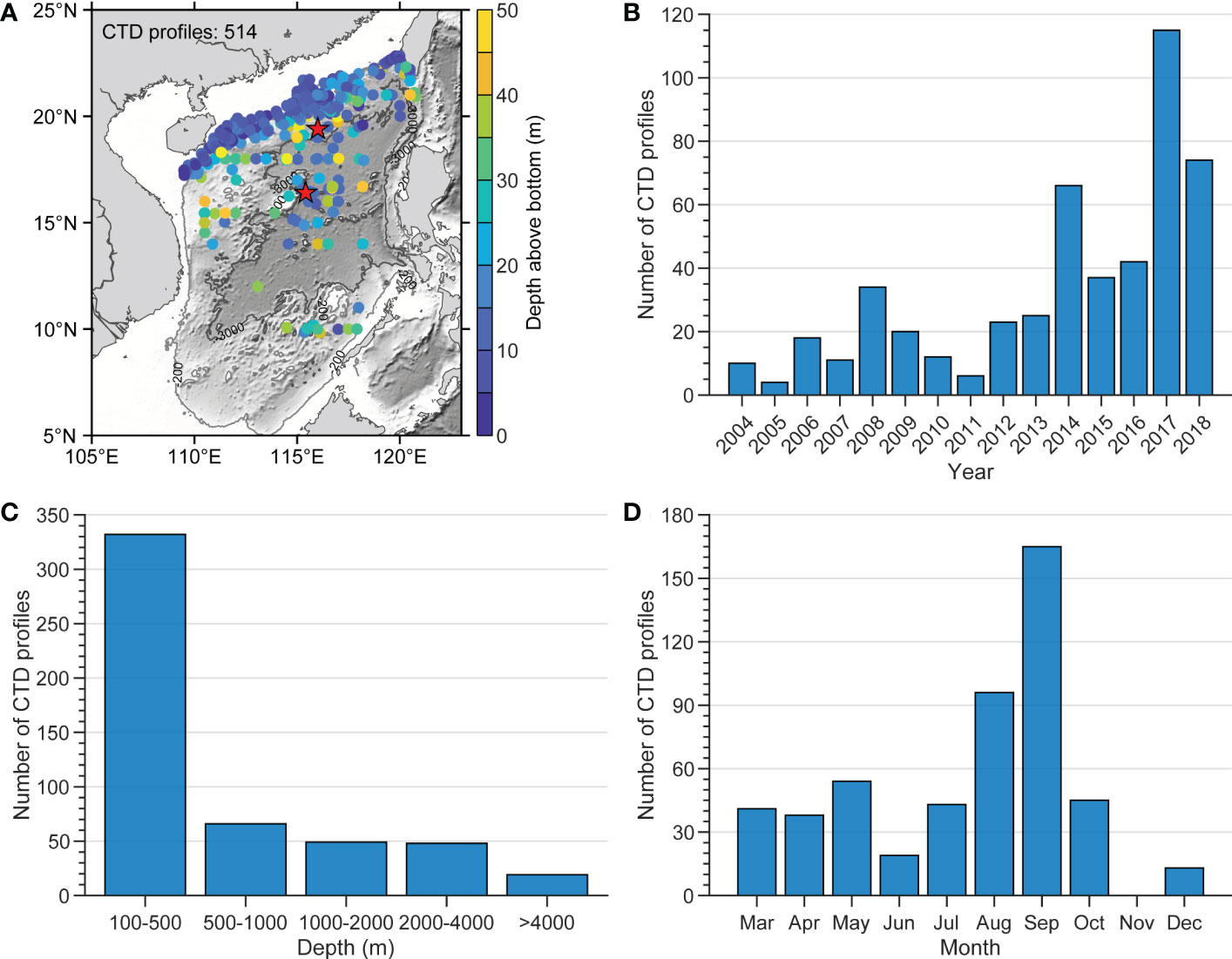
Figure 1 (A) The map of the South China Sea showing the locations of historical observations. The dots are the CTD cast stations and their color indicates the height of the raw data above the bottom. The red stars indicate the locations of the two mooring stations; The CTD observational frequency statistics are displayed by the (B) year, (C) depth, and (D) month.

Given the observational data that has accumulated in the SCS over the past decades, particularly full-depth CTD observations have grown rapidly in recent years (Figure 1B), allowing us to explore the structure of the BML in the SCS in more detail than before. In this study, we investigate the basic spatial-temporal characteristics of the BML from historical hydrological data and mooring observations. Our results suggest that the mean and median H_BML values in the SCS are about 73 m and 56 m, respectively. Those values are smaller than the mean value (154 m) in the SCS as estimated by Li et al. (2022) but larger than the global ocean median value (47 m) as suggested by Huang et al. (2019). In addition, we found that BML is thicker and unstable over the northern continental slope, and is relatively thin and stable over the continental shelf and in the deep-sea region. The possible formation mechanisms for the BML differences between the northern continental slope and deep-sea regions are also discussed in this paper.

2 Data and methods

2.1 CTD data

The historical hydrographic data of full-depth temperature and salinity profiles collected by the SCS open cruises and several research field campaigns during the past 15 years (2004-2018) are used in this study. These data were obtained from a SBE-911plus conductivity-temperature-depth (CTD) system using frequencies between 8–24 Hz. After pre-and post-cruise calibrations, the accuracies of the CTD sensors are 0.0003 S m^-1 for salinity and 0.0018°C for temperature. To get as complete a vertical profile of the BML as possible without damaging the CTD sensors by colliding with the bottom, acoustic altimeters were used in the more recent cruises to monitor the distance of the sensors to the bottom. In this study, only the downcast data that with maximum observed depth less than 50 m from the bottom are used because those data may more easily observe the structure of the BML.

The raw CTD data quality control applied the following criteria: (i) remove CTD profiles where the original information about the station position and/or water depth is missing or incorrect; (ii) because only deeper locations are considered in this study, stations with depths less than 100 m are excluded; (iii) down sample the raw vertical high-resolution to 1 m and apply a 5 m running mean filter to smooth the data. Applying these criteria and after validation, only 514 CTD profiles remained. Nevertheless, these selected CTD data records covered nearly the entire SCS north of 13°N and provided more than adequate coverage of the northern continental slope region of the SCS (Figure 1A). While the majority of the selected CTD profiles were located in depths shallower than 500 m, there were 120 CTD profiles at locations deeper than 1000 m (Figure 1C). Most of those profiles were collected from August and September (Figure 1D) because the routine SCS open cruises were conducted in those two months.

2.2 Mooring observations

Two bottom-anchored moorings were particularly deployed at two sites (Figure 1A) for obtaining time series to characterize the temporal variations of the BML. One was deployed on the northern continental slope of the SCS (M1) and the other was in the deep basin in the western SCS (M2), in the latter of which a previous study had confirmed the existence of a strong deep western boundary current (Zhou et al., 2020). To obtain simultaneous observations, these two moorings were both deployed in August 2017 and recovered in September 2018, collecting a 14-month long time series for use in this study. The moorings had seven RBR-TDs and seven SBE 37 CTDs measuring temperature and pressure near the bottom at M1 and M2, respectively. The accuracies of the RBR-TDs were ±0.002°C for temperature and ±0.05% over the full-scale range for pressure. The accuracies of the SBE 37 CTDs were ±0.002°C for temperature and ±0.1% over the full-scale range for pressure. The design and configuration of the moorings used in this study are shown in Table 1. Since there were no salinity measurements on the M1 mooring, the present study only examines the variation of temperature in the near-bottom regions at the two sites. To explore the low frequency variations of temperature, a 72-h low-pass filter was used to remove the inertial, tidal, and other high-frequency signals (Thomson and Emery, 2014). All data were averaged over an hourly interval.

TABLE 1

Table 1 Experimental mooring design and configuration.

2.3 Additional datasets

To help analyze the potential influence of tidal currents on the distribution of the H_BML, the barotropic tidal currents computed from harmonic constituents provided by the latest TPXO9‐atlas tidal models (Egbert and Erofeeva, 2002) are used to calculate the tidally driven mixing and dissipations of SCS. The TPXO9‐atlas is a 1/30° resolution global model of ocean tides, which represents optimal least squares fit of the Laplace tidal equation to satellite altimetry data. TPXO9 atlas provides the eight major tidal (M2, S2, N2, K2, K1, O1, P1, Q1), three long period (Mf, Mm, 2N2) and three non-linear (M4, MS4, MN4) harmonic constituents. In this study, only the eight most energetic tidal harmonic constituents of the TPXO9‐atlas solution were used to calculate the yearlong (2017) hourly time series of barotropic tidal currents in the SCS.

According to the vertical mixing parameterization scheme as proposed by St. Laurent et al. (2002), which has been applied to estimate the diapycnal mixing induced by internal tides (St. Laurent et al., 2002; Wang et al., 2016; Tan et al., 2022), the turbulent dissipation rate ϵ and diapycnal diffusivity k_v can be calculated as follows:

$\begin{array}{ll}ϵ=(q/\rho )E(x,y)F(z)& (1)\end{array}$

$\begin{array}{ll}{k}_v\simeq \frac{\Gamma ϵ}{N^2}+k_0=\frac{\Gamma qE(x,y)F(z)}{\rho N^2}+k_0& (2)\end{array}$

where Γ is the mixing efficiency taken to be 0.2 (Osborn, 1980), q = 0.3 is the local tidal dissipation efficiency as suggested by St. Laurent et al. (2002), ρ is density of seawater, N² is the squared buoyancy frequency, and k₀ is the background diffusivity (1×10^-5 m² s^-1). F(z) is the function for the vertical structure of the dissipation, chosen tosatisfy energy conservation within an integrated vertical column, ${\displaystyle {\int }_0^{-H}F(z)dz=1}$. Because only the barotropic tidal flow is considered in this study, thus the term F(z) is taken to be 1. E (x, y) is the energy flux per unit area transferred from barotropic to baroclinic tides, formulated as

$\begin{array}{ll}E(x,y)=\frac{1}{2}{\rho }_0{N}_{b}k{h}^2{u}_{bt}^2& (3)\end{array}$

where ρ₀ is the reference density, N_b is the buoyancy frequency at the seafloor, k and h are the wavenumber and amplitude scales for the topographic roughness, respectively. The wavenumber is set to k = 2π/(10 km), we take the horizontal scales of O (10 km) as typical of the roughness. The h² is defined as the variance of bathymetry over a 1/4°×1/4° domain square (using GEBCO_2022 gridded bathymetric dataset). u_bt is the averaged horizontal speed of the barotropic tides over a yearlong time series. In this study, the density of seawater and buoyancy frequency are calculated from the GDEMv3 database (Carnes, 2009).

In addition, a two-dimensional map of the internal tidal dissipation dataset was also used in this study. The dataset consists of global column-integrated maps of internal tide energy sources and sinks with a horizontal resolution of 0.5° × 0.5°. In this dataset, energy sinks are provided for each of M2, S2 and K1 and for “All constituents” (the eight most energetic tidal constituents). The energy sinks are decomposed into five process contributions: (i) dissipation of low modes via wave-wave interactions; (ii) dissipation of low modes scattering by abyssal hills; (iii) dissipation of low modes critical reflection; (iv) dissipation of low modes shoaling; (v) local dissipation of high modes. Units are Watts per square meter. Considering the dissipation of low modes via wave-wave interaction mainly occurs in the stratified water column away from boundary layers (Polzin and McDougall, 2022), thus only the other four processes were used in this study. Detailed information about the dataset and documentation can be found in de Lavergne et al. (2019).

2.4 Identifying the thickness of BML

In this study, a relative variance method is used to identify the H_BML in the SCS. This method is based on the ratio between the standard deviation and the maximum variation of the temperature, salinity, or density profiles above the sea bed; the position of the minimum relative variance is defined as the top of BML (Huang et al., 2018b). The relative variance method is an objective method that determines the H_BML that is less dependent on arbitrary criteria (Huang et al., 2018b). Although the relative variance method was first proposed to identify the surface mixed layer, its performance in determining the H_BML is also superior to other available methods (Huang et al., 2018a). A detailed description of the method and implementation can be found in Huang et al. (2018a) and Huang et al. (2018b).

We use the relative variance method separately on the profiles of potential temperature, salinity, and potential density to obtain three estimated values of the H_BML in each CTD cast. The quality index (QI) defined in Lorbacher et al. (2006) was used to evaluate the quality of the estimate of H_BML, and profiles with QI<0.5 were discarded. It should be noted that there may exist real differences between the three H_BML estimated values, and the value with higher QI is adopted as the observed H_BML. In addition to the formal objective analysis of the H_BML, all profiles used in this study were visually inspected to detect possible errors due to contaminated samples or accidental spikes. Figure 2 shows an example of temperature and salinity profiles collected at 117.06°E, 21.45°N near the Dongsha Islands, where a well-mixed layer clearly exists in the near-bottom zone with an H_BML of about 100 m.

FIGURE 2

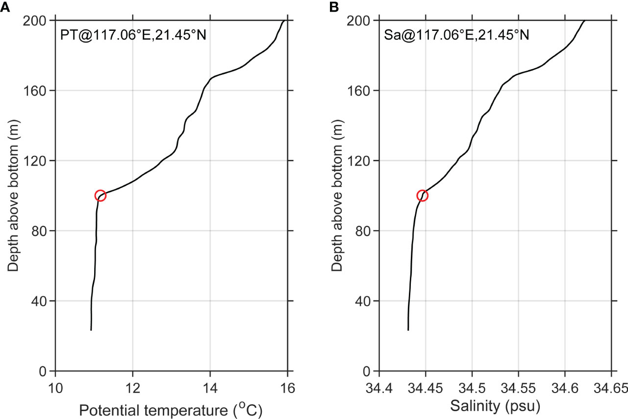
Figure 2 An example of potential temperature (A) and salinity (B) profiles collected near the Dongsha Islands, with the water depth of 443 m. The thickness of the bottom mixed layer is determined to be about 100 m (marked by red circles).

2.5 Estimating the vertical eddy diffusion coefficient

We estimate the vertical eddy diffusion coefficient by using the advection-diffusion equation and mooring observations. Assuming that vertical advection is balanced mainly by vertical diffusion (Munk, 1966), the momentum equation of temperature excluding the source and sink terms, becomes

$\begin{array}{ll}\frac{\partial T}{\partial t}+w\frac{\partial T}{\partial z}=A_z\frac{{\partial }^{2}T}{\partial z^2}& (4)\end{array}$

where T is the potential temperature, t is time, z is the vertical coordinate (positive upward), w and A_z are the vertical velocity and vertical eddy diffusion coefficient, respectively. In Eq. (4), the three terms $\partial T/\partial t$, $\partial T/\partial z$, and ${\partial }^{2}T/\partial z^2$ can be estimated from the mooring observations, thus the unknown values of w and A_z can be estimated from a set of linear equations using the least-square fitting method (Thomson and Emery, 2014).

2.6 The topographic slope and ruggedness

To investigate the distribution of H_BML in the SCS and its sensitivity to ocean topography, two main aspects representing the topographic effects are considered. One is the topographic slope angle (θ) and the other is the topographic ruggedness. The topographic slope angle is defined as the magnitude of the grid topography gradient vector, and use the arc tangent to convert it to an angle. The topographic ruggedness, which measures the degree of irregularity of the topography, is defined by the topographic ruggedness index (TRI), defined by (Riley et al., 1999):

$\begin{array}{ll}TRI={[{\displaystyle \sum {(x_{ij}-x_{00})}^2}]}^{1/2}& (5)\end{array}$

where i and j are the zonal and meridional grid numbers in the specified domain, respectively, and $x_{ij}$ is the elevation of each neighbor cell relative to the center point cell, $x_{00}$. The TRI presents the sum of changes in elevation between a grid cell and its neighboring cells and is equivalent to the standard deviation in two dimensions (Riley et al., 1999). In this study, we calculate the topographic slope and topographic ruggedness on the same 1°×1° spacial domain as that of the bin averaged distribution of H_BML.

3 Results

3.1 The observed H_BML in the SCS

The H_BML computed from the 514 CTD profiles range from 4~255 m, with the mean, median, and one standard deviation being 73 m, 56 m, and 55 m, respectively (Figure 3). The mean and median values are much smaller than the mean H_BML (154 m) that estimated from the 201 full-depth hydrographic profiles by Li et al. (2022), but somewhat larger than the median value (47 m) in the global ocean estimated with full-depth CTD data from the World Ocean Circulation Experiment program (Huang et al., 2019). The probability density distribution of the H_BML (Figure 3) demonstrates that 45% of the H_BML are in the range of 20~80 m, and 27% of the H_BML are thicker than 100 m, with a positive skewness (1.25).

FIGURE 3

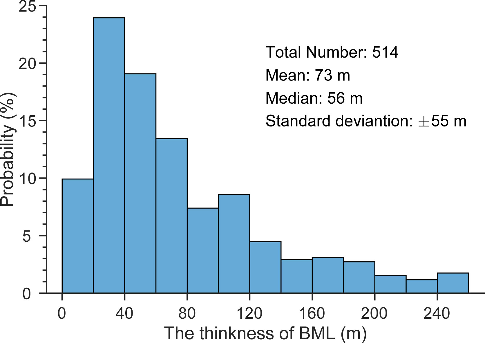
Figure 3 The probability density distribution of BML thickness in the SCS.

The H_BML shows different distribution characteristics with water depth. The thickest averaged H_BML (133 m), with a standard deviation of 72 m, occurs at a depth of ~700 m in the SCS (Figure 4A). The correlation between the H_BML and water depth is positive for water depths shallower than 700 m, and negative for water depths deeper than 700 m. These relationships are quite different from the global distribution presented by Huang et al. (2019), where the H_BML increased exponentially for water depths deeper than 1000 m (the statistics for stations shallower than 1000 m were not presented and stations shallower than 500 m were not considered in their study). These differences between the SCS and the open ocean suggest that the distribution of the H_BML in the SCS may be regulated by more local dynamic factors rather than the general factors in the open ocean.

FIGURE 4

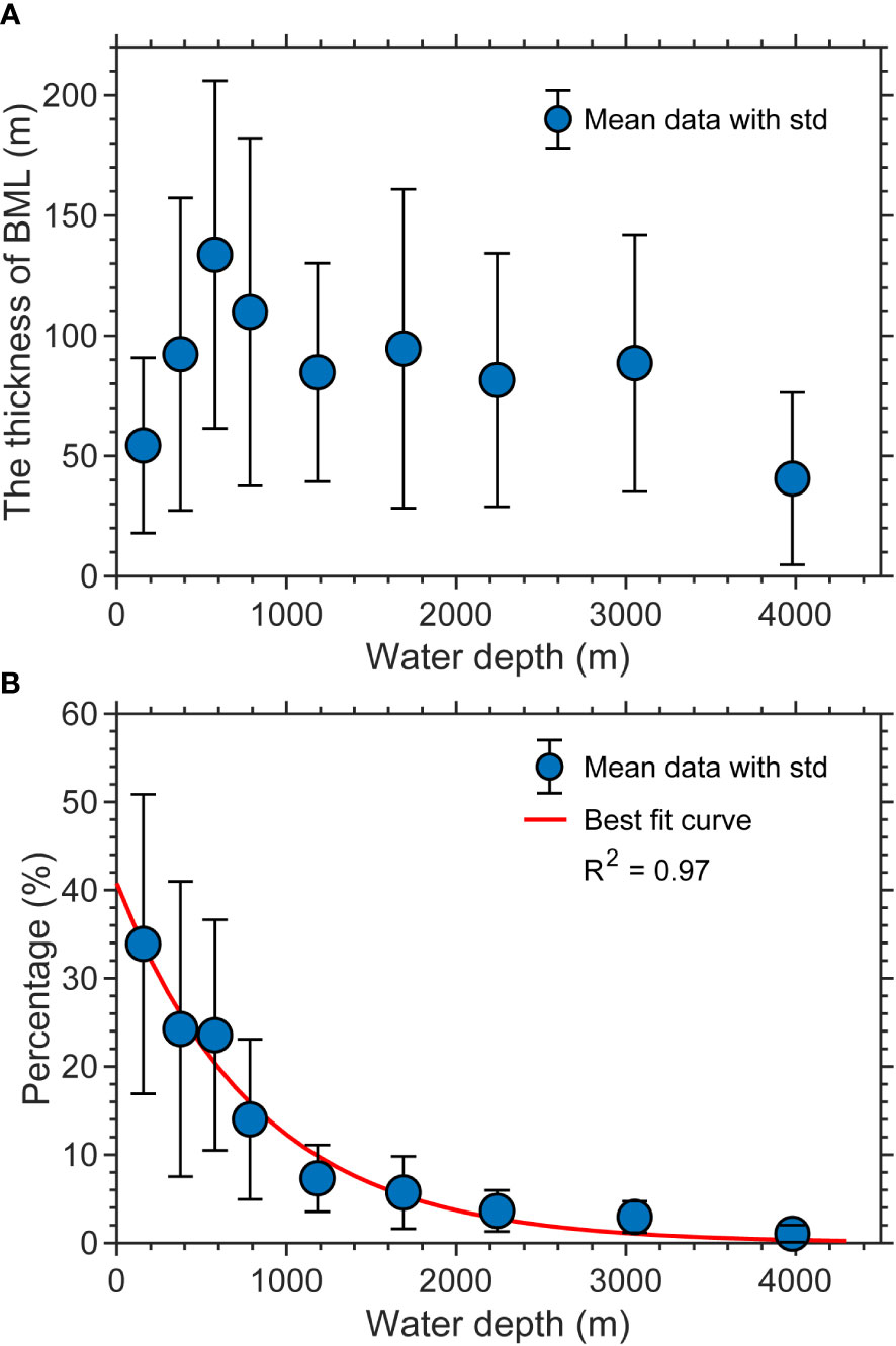
Figure 4 (A) The distribution of the domain-averaged H_BML as a function of the ocean depth; (B) the percentage of BML to the ocean depth as a function of the ocean depth with the least-squares fit superimposed (red curve).

To obtain a quantitative relationship between H_BML and water depth, we calculate the ratio (R_H/D) between the H_BML and the total water depth (D) to evaluate how the H_BML varies as a function of depth (Figure 4B). In general, the R_H/D decreases roughly exponentially with water depth following the least-squares best fit curve:

$\begin{array}{ll}{R}_{H/D}=0.4077\exp (-0.0012D)& (6)\end{array}$

The mean ratio ranges from 10–50% for depths between ~100–700 m, between 5–10% for depths of ~1000 m, and less than 2% for water deeper than 3000 m. All these values are slightly higher than the results estimated in the North Atlantic (Lozovatsky et al., 2008; Lozovatsky and Shapovalov, 2012), suggesting that bottom mixing is more active in the SCS.

To estimate the seasonal variation of H_BML in the SCS, we calculate the median values of the H_BML and its standard deviations in each season. The results show that the H_BML is relatively small in summer, and large in spring and autumn, suggesting the H_BML has obvious seasonal variation in the SCS (Figure 5). Unfortunately, the feature of H_BML in the winter season cannot be described because only few data were collected during the winter.

FIGURE 5

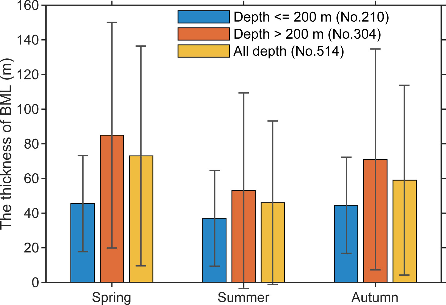
Figure 5 The seasonal averaged values of H_BML and its standard deviations in the SCS based on the CTD observations.

To investigate the spatial distribution of H_BML in the SCS, we project the geographic scatter data in the 1°×1° bins and calculate the median values of H_BML in each grid cell (Figure 6). The results show that the H_BML is thicker (>100 m) on the northern continental slope of SCS, especially in the regions adjacent to the west Luzon Strait and Dongsha Islands, where previous studies have suggested that bottom mixing is enhanced (Tian et al., 2009; Yang et al., 2016; Lu et al., 2021). In contrast, the H_BML is thin over both the continental shelves (around 30–60 m) and the deep-sea regions (around 10–50 m). Despite the limited data in each bin, the variations in the H_BML (calculated by using at least 5 points in the bin) is relatively large on the northern continental slope (not shown), indicating a relatively unstable H_BML over the continental slope regions.

FIGURE 6

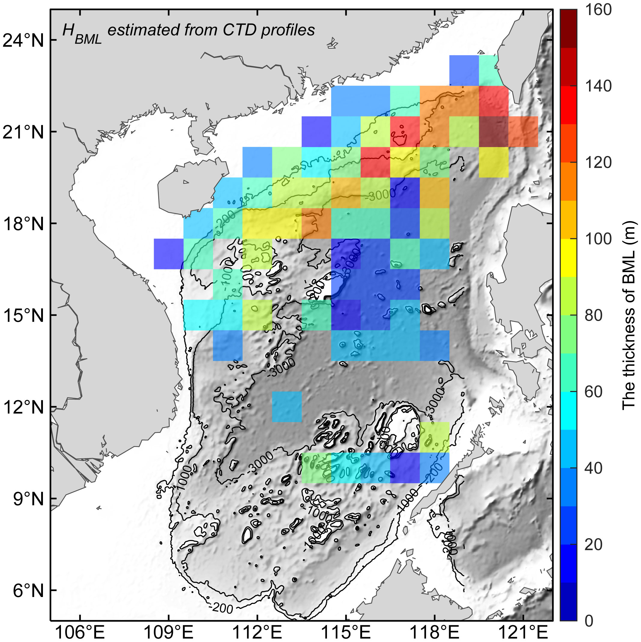
Figure 6 The horizontal distribution of mean BML thickness averaged in 1°×1° bins.

Two deep moorings were deployed to measure the variability of the near-bottom potential temperature over the continental slope (M1) and deep-sea region (M2). Figure 7 shows the temporal variations of the bottom potential temperature and its corresponding gradient. The potential temperature and its variations at the M1 were much larger than that at M2. Their mean potential temperature with the one standard deviation was 2.31 ± 0.04°C and 2.07 ± 0.01°C, respectively. In particular, the mean potential temperature lapse rates (analogous to the “lapse rate” in the atmosphere) calculated from the two moorings were -5.75×10^-4 °C/m and -3.21×10^-4 °C/m, respectively.

FIGURE 7

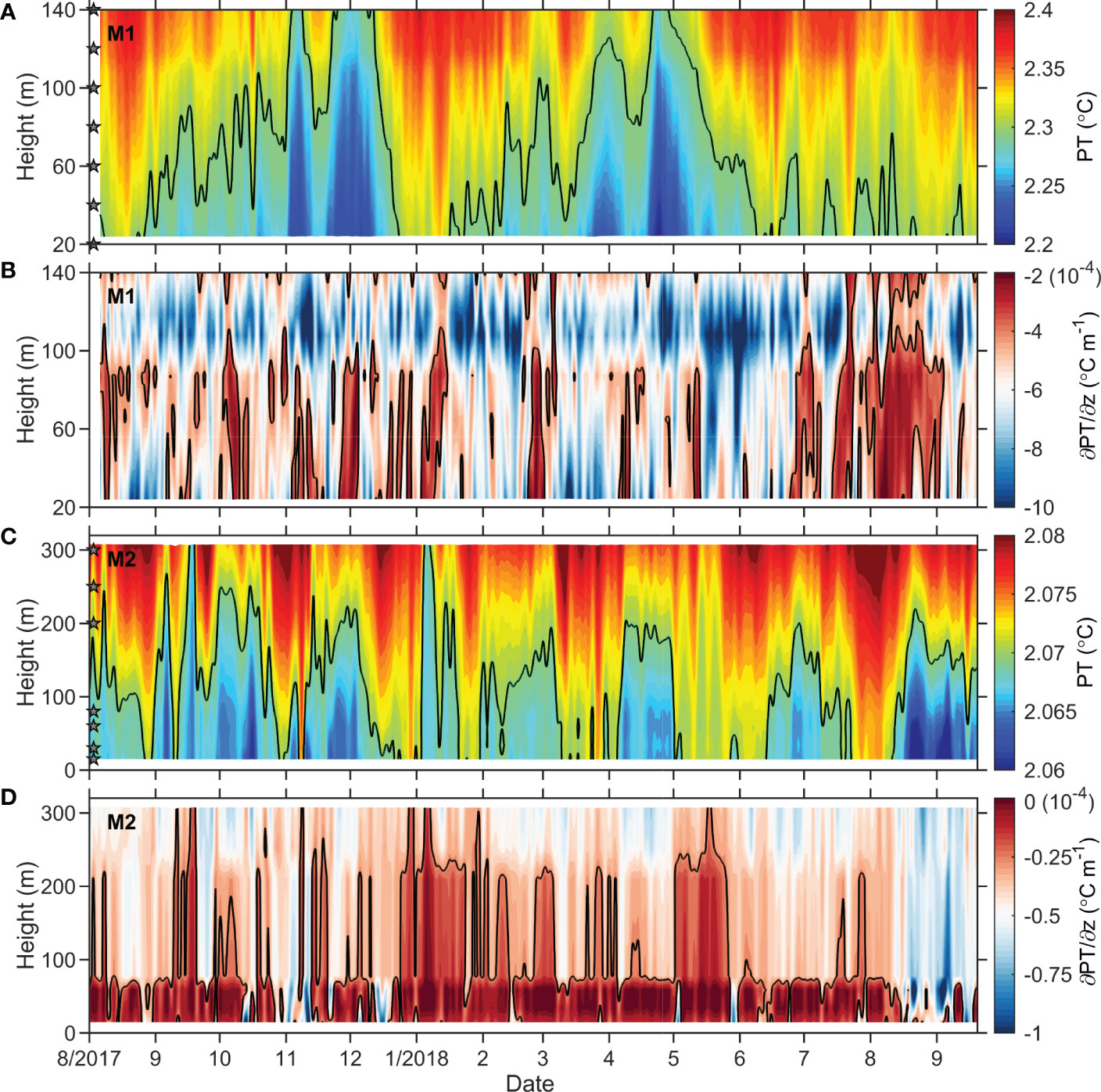
Figure 7 Mooring observations of the near-bottom (A) potential temperature variations and (B) the corresponding vertical temperature gradients at M1; (C, D) are the same as (A, B) but for the M2 station. Black solid lines in (A, C) indicate the contour line of 2.3°C and 2.07°C, respectively; Black solid lines in (B, D) indicate the contour line of -4×10^-4 °C m^-1 and -0.25×10^-4 °C m^-1, respectively. The gray stars in (A, C) indicate the installation positions of the instruments.

Although the differences in the potential temperature profiles between M1 and M2 are significant, quasi-homogeneous layer structures in the near-bottom zone can be clearly seen. During most of the observation period, the homogeneous layer is much thicker at the M1 mooring than that at the M2 mooring. The height of the homogeneous layer appears roughly between 100~120 m above the bottom at M1 and 40~60 m above the bottom at M2. This confirms the earlier observation that the H_BML over the continental slope is thicker than it is in the deep-sea regions. In addition, the structures of the quasi-homogeneous layer at M1 are more complex than that at M2, suggesting that the quasi-homogeneous layer is much unstable at M1 than that at M2. The result is also consistent with the CTD observations that the H_BML over the continental slope is unstable than that in the deep-sea regions.

3.2 The potential formation mechanisms of the BML in the SCS

In the section, we combine the observational results to analyze the potential formation mechanisms of the BML in the SCS, especially focusing on the BML differences between the northern continental slope (M1) and the deep-sea regions (M2). Although it is unclear whether the BML can be regarded as the classic bottom Ekman Layer (Armi and Millard, 1976; Beaulieu and Baldwin, 1998), the velocity shear within the bottom Ekman layer drives stable mixing that keeps the layer unstratified. In bottom Ekman layer dynamics, the turbulent Ekman layer formed above the ocean’s bottom can be expressed as $h\approx 0.4u^{*}/f$, where the u* is friction velocity and f is the Coriolis parameter. In practice, the friction velocity u*, which correlates with bottom currents and bottom drag coefficient (C_d), is not clearly determined from the observations. One simplest procedure to reinterpret the Ekman layer height (h) with friction velocity u* depend on the local mean current and constant drag coefficients (Stahr and Sanford, 1999). Because few current measurements are available, the fluctuations of bottom temperature linked with bottom currents are used to analyze the mixing strength and possible energy sources that influence the structure of the BML.

Spectral analysis of the bottom potential temperatures (using hourly data) shows that variability over the continental slope was dominated by the internal tidal and near-inertial signals, while only low-frequency oscillations (~60 days) were significant in the deep ocean (Figure 8). It is suggested that the differences in the H_BML between the continental slope and deep-sea regions may be caused by different dynamical processes. In the SCS, the internal tides are widely distributed on the continental slope (Alford et al., 2015; Wang et al., 2016), with most of those signals emanating from the Luzon Strait (Zhao, 2014; Alford et al., 2015). The near-inertial signals are likely injected into the upper ocean by typhoon processes (Xu et al., 2013; Zhang et al., 2022) or by other upper ocean mechanisms (Alford et al., 2016). The dominance of these two signals suggests that the internal tidal and near-inertial motions may play the primary roles in the strong mixing along continental slopes (Tian et al., 2009; Wang et al., 2016; Lu et al., 2021). For the deep ocean, the low-frequency oscillations (30-120 days) may be induced by the topographic Rossby waves or the deep ocean eddies, which has been shown in recent observational studies (Zhou et al., 2017; Zhou et al., 2020; Zheng et al., 2021).

FIGURE 8

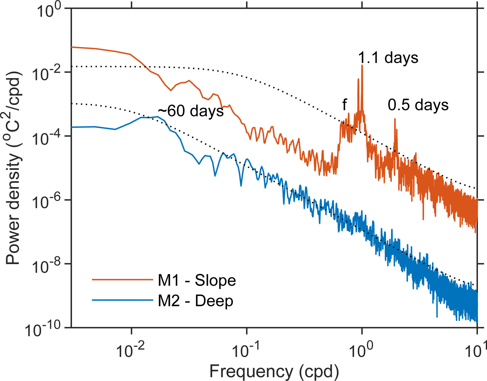
Figure 8 Power spectrum of the near-bottom potential temperature (at 60 m above the bottom) at the M1 (continental slope) and M2 (deep-sea) mooring sites. The dotted lines show the 95% significance level.

To confirm whether the tidally driven mixing and dissipation match the BML distribution pattern in the SCS, we calculated the distribution of baroclinic energy conversion (E), turbulent dissipation rate (ϵ), and diapycnal diffusivity (k_v) in the SCS (see Section 2.3). As expected, the spatial distributions of the depth-integrated E, ϵ, and k_v reveal significant spatial variations (Figures 9A–C). The E, ϵ, and k_v near the Luzon straits and the northern continental slopes usually can exceed 1×10^-3 W m^-1, 1×10^-7 W kg^-1, 1×10^-3 m² s^-1, respectively. The regions with these high values correspond to the areas in which the H_BML is thicker in the SCS (Figure 6). Whereas except some regions with rough topography such as islands, seamounts, and shelf breaks the E, ϵ, and k_v in the central SCS are about one or two orders of magnitude weaker, which corresponds to the thinner H_BML in the SCS (Figure 6). The above typical characteristics of mixing and dissipation pattern match well with the internal tide dissipation as estimated by de Lavergne et al. (2019) (Figures 9D, 10), as well as consistent with the previous observational reports (Tian et al., 2009; Yang et al., 2016; Shang et al., 2017; Lu et al., 2021) and model estimations (Wang et al., 2016). It suggests that the tidal energy is a major source of energy to inducing the strong dissipation and diffusivity, thus influencing the distribution of BML in the SCS.

FIGURE 9

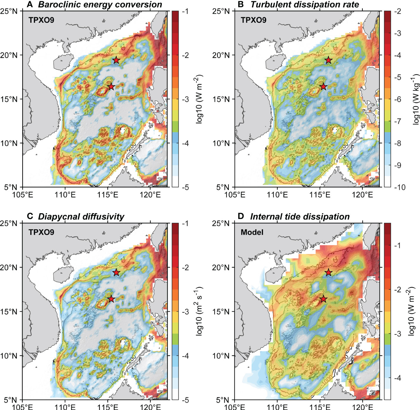
Figure 9 (A) The energy conversion from barotropic to the baroclinic tide, (B) the turbulent dissipation rate, and (C) diapycnal diffusivity as estimated from the TPXO9 tidal model and Equations (1-3). (D) The internal tide dissipation estimated by de Lavergne et al. (2019). Two red stars in each panel indicate the mooring stations.

FIGURE 10

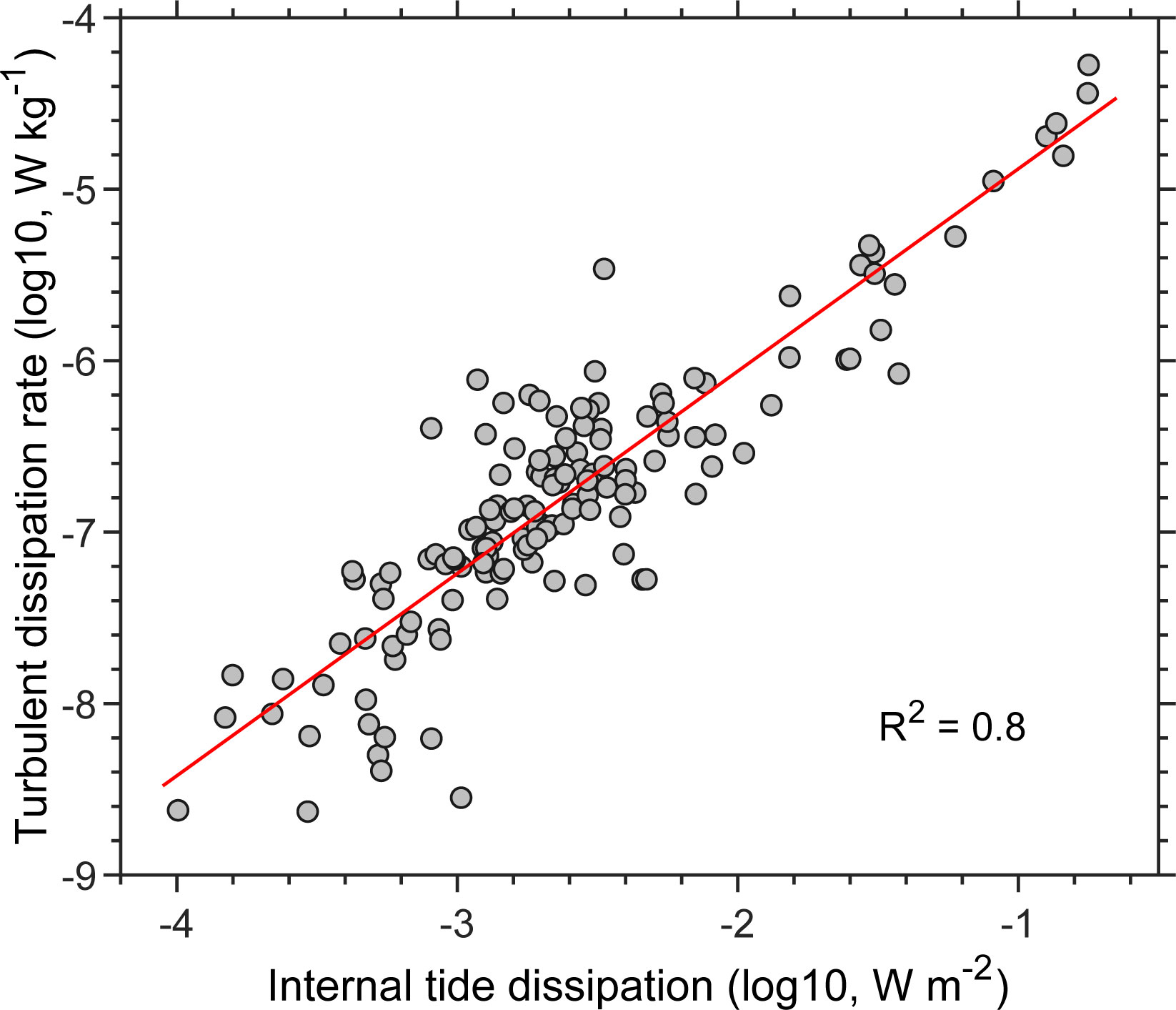
Figure 10 Scatter plots of the turbulent dissipation rate estimated from TPXO9 and the internal tide dissipation suggested by de Lavergne et al. (2019). Both data are averaged in 1°×1° bins.

In addition, the above results reveal the diapycnal diffusivity at M1 is higher than that at M2, which can also be confirmed by the mooring observations (see Section 2.5). The calculation shows that the estimated average eddy diffusion coefficient varies between 1.0×10^-6 to 5.3×10^-3 m² s^-1 at M1 and -2.3×10^-7 to 5×10^-3 m² s^-1 at M2. The estimated mean eddy diffusion coefficients were 1.3×10^-3 m s^-1 and 8.4×10^-4 m² s^-1 at M1 and M2, respectively. These values are in agreement with practical observations estimated from the Thorpe-scale method and direct observations in previous studies (Yang et al., 2016; Shang et al., 2017; Lu et al., 2021), suggesting that the bottom vertical mixing over the continental slope (M1) is stronger than that in the deep-sea regions (M2), which may explain why the H_BML over the continental slope is thicker than in the deep-sea regions.

We analyze other potential factors that may contribute to the bottom mixing and their distribution differences in the SCS. CTD and mooring observations are used to consider the roles of topography, internal tidal dissipation, and density stratification in the distribution of H_BML between the continental slope (M1) and deep-sea regions (M2). The results in Figures 11A–C show that the H_BML increases with increasing topographic slope, topographic ruggedness, and internal tidal dissipation. The typical values of the topographic slope, topographic ruggedness, and internal tidal dissipation are all larger at M1 than that at M2, and likely all contribute to the thicker H_BML over the continental slope. Figure 11D shows the H_BML as a function of the buoyancy frequency estimated within the BML. This result shows no monotonic relationship between the H_BML and the buoyancy frequency as suggested by Huang et al. (2019), in which they showed that the H_BML tends to be thinner with stronger stratification. However, our results suggest that the stratification may not be important for determining the BML differences between the continental slope and the deep-sea regions. In other words, the dominant factors controlling the distribution of the H_BML in the SCS are dynamic rather than thermodynamic.

FIGURE 11

Figure 11 The distribution of H_BML as a function of (A) topographic slope, (B) topographic ruggedness index, (C) internal tidal dissipation, and (D) buoyancy frequency. Gray dots and error bars denote the average values with one standard deviation. Blue and red dots indicate the mean value near the continental slope (M1) and deep-sea regions (M2), respectively. The best fits are plotted as a black curve in panels (A–C). Note that the averaged-buoyancy frequency in panel (D) was estimated within the BML with the thickness of BML determined by Eq. (6).

Taken together, we conclude that the dynamic processes over the northern continental slope controlling the BML are the energetic, high-frequency forcing, together with the large slope and steep topography, which combine to cause strong tidal energy dissipation and vertical mixing near the bottom in these regions. As a result, the BML on the northern continental slope is relatively thick. Conversely, in the deep-sea regions, the dynamic processes are low-frequency, and the topographic roughness and slope are relatively smooth and gentle, so that the tidal energy dissipation and bottom vertical mixing are considerably weaker, resulting in a relatively thin BML in the deep-sea regions.

4 Summary and discussion

In this study, we combined historical hydrological data and observations from two in-situ moorings to investigate the spatial-temporal characteristics of the BML in the SCS. In general, the H_BML is thicker over the northern continental slope, especially in the region to the west of the Luzon Strait and Dongsha Islands, where the median H_BML is thicker than 100 m. In contrast, the H_BML is relatively thin over the continental shelf and in deep-sea regions, with median thicknesses of around 30–60 m and 10–50 m, respectively. The values for the mean, median, and standard deviation of H_BML in these regions were 73 m, 56 m, and 55m, respectively. Further analysis revealed that the differences in the H_BML between the northern continental slope and deep-sea regions are due to the different dynamic processes, topographic features, internal tidal dissipation, and bottom vertical mixing between these two regions. Specifically, the high-frequency energetic dynamic processes and steep topography (large topographic slope and roughness), cause stronger tidal dissipation and bottom vertical mixing over the continental slope, leading to a thicker BML there. Conversely, in the deep ocean, the dynamic processes are low-frequency and lower energy, and the topography is relatively smooth (small topographic slope and roughness), leading to relatively weak tidal dissipation and vertical mixing near the bottom, and resulting in a thinner BML in the deep-sea regions.

To further explore the distribution of the H_BML over the entire SCS, we derived a statistical relationship (shown in Figure 11C) between the H_BML and the tidal dissipation. The results show that the thickest estimated H_BML appears to the west of the Luzon Strait, the continental slope (especially the northern continental slope), and surrounding islands, seamounts, and shelf breaks (Figure 12). In particular, the thick H_BML features around the Zhongsha Island Chain as suggested by Li et al. (2022) can be also seen in Figure 12, but the reconstructed H_BML value is thinner than their results. Furthermore, the thicker H_BML over the northern continental slope is also apparent in the average thicknesses for each latitude (Figure 13). Both the magnitude and the spatial pattern of H_BML are in good agreement with the observed values from the CTD profiles (see Figures 6, 12), suggesting that tidal dissipation can be a useful factor to predict the H_BML in the SCS.

FIGURE 12

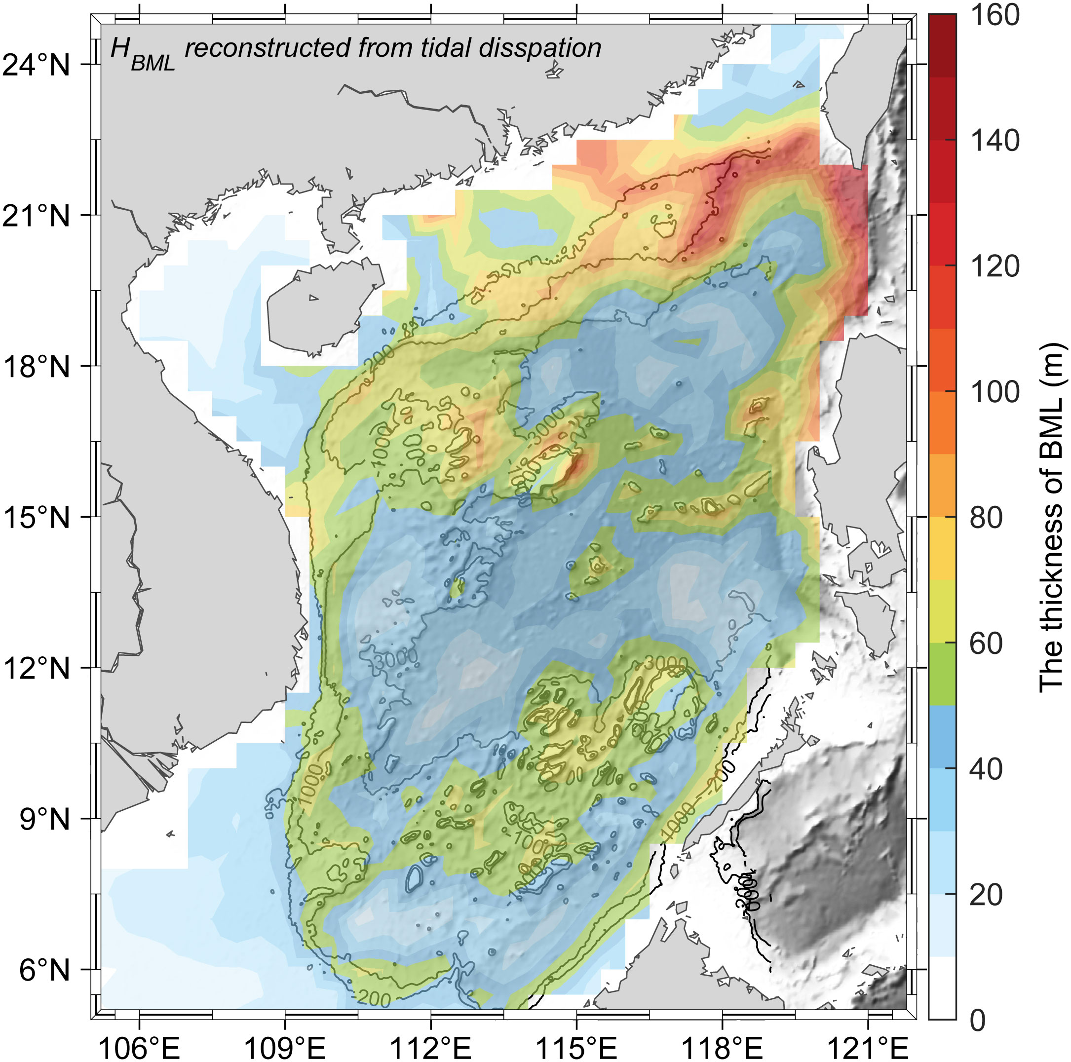
Figure 12 The spatial distribution of the reconstructed H_BML in the SCS by the statistical relationship in Figure 11C. Two red stars indicate the mooring stations.

FIGURE 13

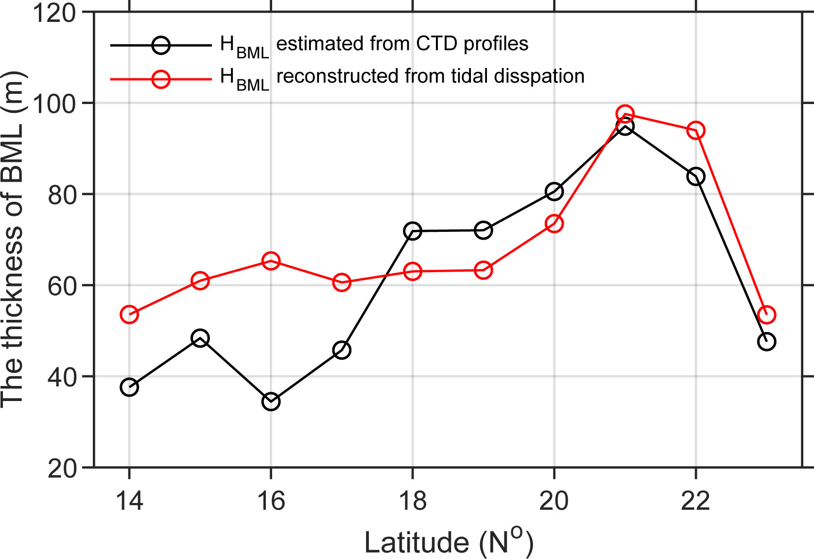
Figure 13 Comparison of the latitudinal distribution of H_BML estimated from the CTD profilers and reconstructed values.

According to de Lavergne et al. (2019), several mechanisms contribute to the tidal dissipation which may have different effects on the distribution of the H_BML. Developing a better assessment of the relative contributions of the different tidal dissipation mechanisms will be important for improving the prediction of the BML’s distribution in the SCS. This would be an important goal of future work in this area. It should be noted that the interactions between currents and topography are very complex, thus more factors that affect the behavior of the BML should be also considered in the future.

The results of this study provide a preliminary description of the BML in the SCS from the observations. We hope our results will be useful for improving our understanding of the BML dynamics in the SCS and may provide observational evidence to refine the BML parameterization in ocean circulation models. However, improving our knowledge of the fine structure and obtaining a longer observational record of BML is still urgently required for future work.

Data availability statement

The GEBCO gridded bathymetry data is available at: https://www.gebco.net. The CTD and moorings data that supporting the conclusions of this article will be made available by the authors, upon reasonable request.

Author contributions

WL conceived the study, performed the data analysis, and wrote the manuscript. GW initiated the idea of the study. All authors contributed to the analysis of the results and editing of the manuscript. All authors contributed to the article and approved the submitted version.

Funding

This work is supported by the National Natural Science Foundation of China (42030405, 42076018, 42106010).

Acknowledgments

The authors are grateful to the scientists, captains and crews of the R/Vs Shiyan 1, Shiyan 3, Dongfanghong 2, Dongfanghong 3, and Jia Geng for their long-term observation efforts, and to the Open Research Cruise of the South China Sea supported by NSFC Shiptime Sharing Projects. The authors would like to thank Prof. Zhijin Li and two reviewers for their helpful and constructive comments on the earlier revision of this manuscript.

Conflict of interest

The authors declare that the research was conducted in the absence of any commercial or financial relationships that could be construed as a potential conflict of interest.

Publisher’s note

All claims expressed in this article are solely those of the authors and do not necessarily represent those of their affiliated organizations, or those of the publisher, the editors and the reviewers. Any product that may be evaluated in this article, or claim that may be made by its manufacturer, is not guaranteed or endorsed by the publisher.

References

Alford M. H., Mackinnon J. A., Simmons H. L., Nash J. D. (2016). Near-inertial internal gravity waves in the ocean. Annu. Rev. Mar. Sci. 8, 95–123. doi: 10.1146/annurev-marine-010814-015746

CrossRef Full Text | Google Scholar

Alford M. H., Peacock T., Mackinnon J. A., Nash J. D., Buijsman M. C., Centuroni L. R., et al. (2015). The formation and fate of internal waves in the south China Sea. Nature 521, 65–69. doi: 10.1038/nature14399

PubMed Abstract | CrossRef Full Text | Google Scholar

Armi L., Millard R. C. (1976). The bottom boundary layer of the deep ocean. J. Geophys. Res. 81, 4983–4990. doi: 10.1029/JC081i027p04983

CrossRef Full Text | Google Scholar

Beaulieu S., Baldwin R. (1998). Temporal variability in currents and the benthic boundary layer at an abyssal station off central California. Deep-Sea Res. Part II Top. Stud. Oceanogr. 45, 587–615. doi: 10.1016/S0967-0645(97)00095-7

CrossRef Full Text | Google Scholar

Carnes M. R. (2009). Description and evaluation of GDEM-V3.0. Naval Res. Lab. Tech. Rep. 21. NRL/MR/7330-09-9165: Washington, D. C.

Google Scholar

Chen G. X., Hou Y. J., Chu X. Q. (2011). Mesoscale eddies in the south China Sea: Mean properties, spatiotemporal variability, and impact on thermohaline structure. J. Geophys. Res. Oceans 116, C06018. doi: 10.1029/2010JC006716

CrossRef Full Text | Google Scholar

de Lavergne C., Falahat S., Madec G., Roquet F., Nycander J., Vic C. (2019). Toward global maps of internal tide energy sinks. Ocean Modell. 137, 52–75. doi: 10.1016/j.ocemod.2019.03.010

CrossRef Full Text | Google Scholar

de Lavergne C., Madec G., Capet X., Maze G., Roquet F. (2016). Getting to the bottom of the ocean. Nat. Geosci. 9, 857–858. doi: 10.1038/ngeo2850

CrossRef Full Text | Google Scholar

Dyer K. R., Soulsby R. L. (1988). Sand transport on the continental shelf. Annu. Rev. Fluid Mech. 20, 295–324. doi: 10.1146/annurev.fl.20.010188.001455

CrossRef Full Text | Google Scholar

Egbert G. D., Erofeeva S. Y. (2002). Efficient inverse modeling of barotropic ocean tides. J. Atmos. Oceanic Technol. 19, 183–204. doi: 10.1175/1520-0426(2002)019%3C0183:EIMOBO%3E2.0.CO;2

CrossRef Full Text | Google Scholar

Fox-Kemper B., Adcroft A., Böning C. W., Chassignet E. P., Curchitser E., Danabasoglu G., et al. (2019). Challenges and prospects in ocean circulation models. Front. Mar. Sci. 6. doi: 10.3389/fmars.2019.00065

CrossRef Full Text | Google Scholar

Grant W. D., Madsen O. S. (1986). The continental-shelf bottom boundary layer. Annu. Rev. Fluid Mech. 18, 265–305. doi: 10.1146/annurev.fl.18.010186.001405

CrossRef Full Text | Google Scholar

Greenewalt D., Gordon C. M. (1978). Short-term variability in the bottom boundary layer of the deep ocean. J. Geophys. Res. 83, 4713–4716. doi: 10.1029/JC083iC09p04713

CrossRef Full Text | Google Scholar

Hayes S. P. (1979). “Benthic current observations at DOMES sites a, b, and c in the tropical north pacific ocean,” in Marine geology and oceanography of the pacific manganese nodule province. Eds. Bischoff J. L., Piper D. Z. (Boston: Springer), 83–112. doi: 10.1007/978-1-4684-3518-4_3

CrossRef Full Text | Google Scholar

Huang P.-Q., Cen X.-R., Guo S.-X., Lu Y.-Z., Zhou S.-Q., Qiu X.-L., et al. (2021). Variance of bottom water temperature at the continental margin of the northern south China Sea. J. Geophys. Res. Oceans 126, e2020JC015843. doi: 10.1029/2019JC015843

CrossRef Full Text | Google Scholar

Huang P.-Q., Cen X.-R., Lu Y.-Z., Guo S.-X., Zhou S.-Q. (2018a). An integrated method for determining the oceanic bottom mixed layer thickness based on WOCE potential temperature profiles. J. Atmos. Oceanic Technol. 35, 2289–2301. doi: 10.1175/JTECH-D-18-0016.1

CrossRef Full Text | Google Scholar

Huang P.-Q., Cen X.-R., Lu Y.-Z., Guo S.-X., Zhou S.-Q. (2019). Global distribution of the oceanic bottom mixed layer thickness. Geophys. Res. Lett. 46, 1547–1554. doi: 10.1029/2018GL081159

CrossRef Full Text | Google Scholar

Huang P.-Q., Lu Y.-Z., Zhou S.-Q. (2018b). An objective method for determining ocean mixed layer depth with applications to WOCE data. J. Atmos. Oceanic Technol. 35, 441–458. doi: 10.1175/JTECH-D-17-0104.1

CrossRef Full Text | Google Scholar

Hull T., Johnson M., Greenwood N., Kaiser J. (2020). Bottom mixed layer oxygen dynamics in the celtic Sea. Biogeochemistry 149, 263–289. doi: 10.1007/s10533-020-00662-x

CrossRef Full Text | Google Scholar

Li J., Yang Q., Sun H., Zhao W., Tian J. (2022). Spatial variation of bottom mixed layer in the south China Sea and a potential mechanism. Prog. Oceanogr. 206, 102856. doi: 10.1016/j.pocean.2022.102856

CrossRef Full Text | Google Scholar

Lorbacher K., Dommenget D., Niiler P. P., Köhl A. (2006). Ocean mixed layer depth: A subsurface proxy of ocean-atmosphere variability. J. Geophys. Res. Oceans 111, C07010. doi: 10.1029/2003JC002157

CrossRef Full Text | Google Scholar

Lozovatsky I. D., Fernando H. J. S., Shapovalov S. M. (2008). Deep-ocean mixing on the basin scale: Inference from north Atlantic transects. Deep Sea Res. Part I Oceanogr. Res. Pap. 55, 1075–1089. doi: 10.1016/j.dsr.2008.05.003

CrossRef Full Text | Google Scholar

Lozovatsky I. D., Shapovalov S. M. (2012). Thickness of the mixed bottom layer in the northern Atlantic. Oceanology 52, 447–452. doi: 10.1134/S0001437012010134

CrossRef Full Text | Google Scholar

Lu Y.-Z., Cen X.-R., Guo S.-X., Qu L., Huang P.-Q., Shang X.-D., et al. (2021). Spatial variability of diapycnal mixing in the south China Sea inferred from density overturn analysis. J. Phys. Oceanogr. 51, 3417–3434. doi: 10.1175/JPO-D-20-0241.1

CrossRef Full Text | Google Scholar

Munk W. H. (1966). Abyssal recipes. Deep-Sea Res. 13, 707–730. doi: 10.1016/0011-7471(66)90602-4

CrossRef Full Text | Google Scholar

Munk W., Wunsch C. (1998). Abyssal recipes II: energetics of tidal and wind mixing. Deep-Sea Res. Part I Oceanogr. Res. Pap. 45, 1977–2010. doi: 10.1016/S0967-0637(98)00070-3

CrossRef Full Text | Google Scholar

Osborn T. R. (1980). Estimates of the local rate of vertical diffusion from dissipation measurements. J. Phys. Oceanogr. 10, 83–89. doi: 10.1175/1520-0485(1980)010%3C0083:EOTLRO%3E2.0.CO;2

CrossRef Full Text | Google Scholar

Peter M., Garrett C. (2004). Near-boundary processes and their parameterization. Oceanography 17, 107–116. doi: 10.5670/oceanog.2004.75

CrossRef Full Text | Google Scholar

Polzin K. L., McDougall T. J. (2022). “Mixing at the ocean's bottom boundary,” in Ocean mixing. Eds. Meredith M., Naveira Garabato A. (Cambridge: Elsevier), 145–180. doi: 10.1016/B978-0-12-821512-8.00014-1

CrossRef Full Text | Google Scholar

Quan Q., Cai Z., Jin G., Liu Z. (2021). Topographic rossby waves in the abyssal south China Sea. J. Phys. Oceanogr. 51, 1795–1812. doi: 10.1175/JPO-D-20-0187.1

CrossRef Full Text | Google Scholar

Riley S. J., Degloria S. D., Elliot R. (1999). A terrain ruggedness index that quantifies topographic heterogeneity. Interm. J. Scie. 5, 23–27.

Google Scholar

Saunders P. M., Richards K. J. (1985). Benthic boundary layer- IOS observational and modelling programme: Final report (Wormley, (UK: Institute of Oceanographic Science), 61.

Google Scholar

Shang X.-D., Liang C.-R., Chen G.-Y. (2017). Spatial distribution of turbulent mixing in the upper ocean of the south China Sea. Ocean Sci. 13, 503–519. doi: 10.5194/os-13-503-2017

CrossRef Full Text | Google Scholar

Stahr F. R., Sanford T. B. (1999). Transport and bottom boundary layer observations of the north Atlantic deep Western boundary current at the Blake outer ridge. Deep-Sea Res. Part II Top. Stud. Oceanogr. 46, 205–243. doi: 10.1016/S0967-0645(98)00101-5

CrossRef Full Text | Google Scholar

St. Laurent L. C., Simmons H. L., Jayne S. R. (2002). Estimating tidally driven mixing in the deep ocean. Geophys. Res. Lett. 29, 2106. doi: 10.1029/2002GL015633

CrossRef Full Text | Google Scholar

Tan J., Chen X., Meng J., Liao G., Hu X., Du T. (2022). Updated parameterization of internal tidal mixing in the deep ocean based on laboratory rotating tank experiments. Deep Sea Res. Part II Top. Stud. Oceanogr. 202, 105141. doi: 10.1016/j.dsr2.2022.105141

CrossRef Full Text | Google Scholar

Thomson R. E., Emery W. J. (2014). Data analysis methods in physical oceanography. 3rd Edition (Oxford: Elsevier).

Google Scholar

Thorpe S. A. (1987). Current and temperature variability on the continental slope. Philos. Trans. R. Soc Lond. A 323, 471–517. doi: 10.1098/rsta.1987.0100

CrossRef Full Text | Google Scholar

Thorpe S. A. (1988). The dynamics of the boundary layers of the deep ocean. Sci. Prog. 72, 189–206.

Google Scholar

Tian J., Yang Q., Zhao W. (2009). Enhanced diapycnal mixing in the south China Sea. J. Phys. Oceanogr. 39, 3191–3203. doi: 10.1175/2009JPO3899.1

CrossRef Full Text | Google Scholar

Trowbridge J. H., Lentz S. J. (2018). The bottom boundary layer. Annu. Rev. Mar. Sci. 10, 397–420. doi: 10.1146/annurev-marine-121916-063351

CrossRef Full Text | Google Scholar

Wang X., Peng S., Liu Z., Huang R. X., Qian Y.-K., Li Y. (2016). Tidal mixing in the south China Sea: an estimate based on the internal tide energetics. J. Phys. Oceanogr. 46, 107–124. doi: 10.1175/JPO-D-15-0082.1

CrossRef Full Text | Google Scholar

Wang J., Shu Y., Wang D., Xie Q., Wang Q., Chen J., et al. (2021). Observed variability of bottom-trapped topographic rossby waves along the slope of the northern south China Sea. J. Geophys. Res. Oceans 126, e2021JC017746. doi: 10.1029/2021JC017746

CrossRef Full Text | Google Scholar

Wang G., Su J., Chu P. C. (2003). Mesoscale eddies in the south China Sea observed with altimeter data. Geophys. Res. Lett. 30, 2121. doi: 10.1029/2003GL018532

CrossRef Full Text | Google Scholar

Weatherly G. L., Martin P. L. (1978). On the structure and dynamics of oceanic bottom boundary layer. J. Phys. Oceanogr. 8, 557–570. doi: 10.1175/1520-0485(1978)008%3C0557:OTSADO%3E2.0.CO;2

CrossRef Full Text | Google Scholar

Weatherly G. L., Niiler P. P. (1974). Bottom homogeneous layers in the Florida current. Geophys. Res. Lett. 1, 316–319. doi: 10.1029/GL001i007p00316

CrossRef Full Text | Google Scholar

Wunsch C., Hendry R. (1972). Array measurements of the bottom boundary layer and the internal wave field on the continental slope. Geophys. Astro. Fluid 4, 101–145. doi: 10.1080/03091927208236092

CrossRef Full Text | Google Scholar

Xu Z., Yin B., Hou Y., Xu Y. (2013). Variability of internal tides and near-inertial waves on the continental slope of the northwestern south China Sea. J. Geophys. Res. Oceans 118, 197–211. doi: 10.1029/2012JC008212

CrossRef Full Text | Google Scholar

Yang Q., Zhao W., Liang X., Tian J. (2016). Three-dimensional distribution of turbulent mixing in the south China Sea. J. Phys. Oceanogr. 46, 769–788. doi: 10.1175/JPO-D-14-0220.1

CrossRef Full Text | Google Scholar

Zhang H., Xie X., Yang C., Qi Y., Tian D., Xu J., et al. (2022). Observed impact of typhoon mangkhut, (2018) on a continental slope in the south China Sea. J. Geophys. Res. Oceans 127, e2022JC018432. doi: 10.1029/2022JC018432

CrossRef Full Text | Google Scholar

Zhao Z. (2014). Internal tide radiation from the Luzon strait. J. Geophys. Res. Oceans 119, 5434–5448. doi: 10.1002/2014JC010014

CrossRef Full Text | Google Scholar

Zheng H., Zhu X.-H., Zhang C., Zhao R., Zhu Z.-N., Liu Z.-J. (2021). Propagation of topographic rossby waves in the deep basin of the south China Sea based on abyssal current observations. J. Phys. Oceanogr. 51, 2783–2791. doi: 10.1175/JPO-D-21-0051.1

CrossRef Full Text | Google Scholar

Zhou S. Q., Lu Y. Z. (2013). Characterization of double diffusive convection steps and heat budget in the deep Arctic ocean. J. Geophys. Res. Oceans 118, 6672–6686. doi: 10.1002/2013JC009141

CrossRef Full Text | Google Scholar

Zhou M., Wang G., Liu W., Chen C. (2020). Variability of the observed deep western boundary current in the south China Sea. J. Phys. Oceanogr. 50, 2953–2963. doi: 10.1175/JPO-D-20-0013.1

CrossRef Full Text | Google Scholar

Zhou C., Zhao W., Tian J., Zhao X., Zhu Y., Yang Q., et al. (2017). Deep western boundary current in the south China Sea. Sci. Rep. 7, 9303. doi: 10.1038/s41598-017-09436-2

PubMed Abstract | CrossRef Full Text | Google Scholar

Zulberti A. P., Jones N. L., Rayson M. D., Ivey G. N. (2022). Mean and turbulent characteristics of a bottom mixing-layer forced by a strong surface tide and large amplitude internal waves. J. Geophys. Res. Oceans 127, e2020JC017055. doi: 10.1029/2020JC017055

CrossRef Full Text | Google Scholar