Insight into best practices: a review of long-term monitoring of the rocky intertidal zone of the Northeast Pacific Coast

Kaplanis, Nikolas J.

doi:10.3389/fmars.2023.1182562

ORIGINAL RESEARCH article

Front. Mar. Sci., 18 October 2023

Sec. Marine Ecosystem Ecology

Volume 10 - 2023 | https://doi.org/10.3389/fmars.2023.1182562

Insight into best practices: a review of long-term monitoring of the rocky intertidal zone of the Northeast Pacific Coast

Nikolas J. Kaplanis^*

Department of Ecology and Evolutionary Biology, University of California, Santa Cruz, Santa Cruz, CA, United States

On the shores of the Northeast Pacific Coast, research programs have monitored the rocky intertidal zone for multiple decades across thousands of kilometers, ranking among the longest-term and largest-scale ecological monitoring programs in the world. These programs have produced powerful datasets using simple field methods, and many are now capitalizing on modern field-sampling technology and computing power to collect and analyze biological information at increasing scale and resolution. Considering its depth, breadth, and cutting-edge nature, this research field provides an excellent case study for examining the design and implementation of long-term, large-scale ecological monitoring. I curated literature and interviewed 25 practitioners to describe, in detail, the methods employed in 37 community-level surveys by 18 long-term monitoring programs on the Northeast Pacific Coast, from Baja California, México, to Alaska, United States of America. I then characterized trade-offs between survey design components, identified key strengths and limitations, and provided recommendations for best practices. In doing so, I identified data gaps and research priorities for sustaining and improving this important work. This analysis is timely, especially considering the threat that climate change and other anthropogenic stressors present to the persistence of rocky intertidal communities. More generally, this review provides insight that can benefit long-term monitoring within other ecosystems.

Introduction

Long-term monitoring (LTM) of ecosystems is inherently challenging (Hinds, 1984; Andrew and Mapstone, 1987; Wiens, 1989; Levin, 1992; Lindenmayer and Likens, 2010; Muller et al., 2010). Field sampling and maintaining funding is logistically difficult (Caughlan and Oakley, 2001; Muller et al., 2010). Although sampling design guidelines are available, the idiosyncratic nature of ecosystems means that no single design is the best option for characterizing all field sites; a sampling design can over sample one location while under sampling others (Lindenmayer and Likens, 2010; Montes et al., 2021). Sampling design choices are influenced by many factors. Studies may be tradition bound, selecting sampling units and approaches a priori rather than empirically evaluating the appropriate scale or replication for the particular question of interest (Hawkins and Hartnoll, 1983; Andrew and Mapstone, 1987; Wiens, 1989; Miller and Ambrose, 2000; Underwood, 2000; Denny et al., 2004). Assuming finite availability of funding and time, as the temporal duration or spatial extent of a study increases, temporal and spatial sampling resolution must decrease (Wiens, 1989; Levin, 1992; Estes et al., 2018, see Table 1 for sampling design terms). Optimum sample size depends on the level of precision desired, but also on factors including the parameter measured, whether units are fixed or randomly placed, density of the population or community sampled, size of sampling units, and personnel and funding available (Hartnoll and Hawkins, 1980; Hawkins and Hartnoll, 1983; Andrew and Mapstone, 1987; Kingsford and Battershill, 1998; Murray et al., 2006; Hoffmann et al., 2019; Montes et al., 2021). Regardless of their extent and nature, trade-offs force ecologists to make tough decisions regarding the distribution of sampling effort for LTM. This deserves attention because sampling design determines which patterns are apparent, and the variation observed in community composition across space and through time is dependent upon the scale of description (Andrew and Mapstone, 1987; Wiens, 1989; Levin, 1992; Estes et al., 2018). Therefore, one must carefully consider appropriate sampling units, their replication, and their arrangement in space and time when implementing LTM in any ecosystem.

TABLE 1

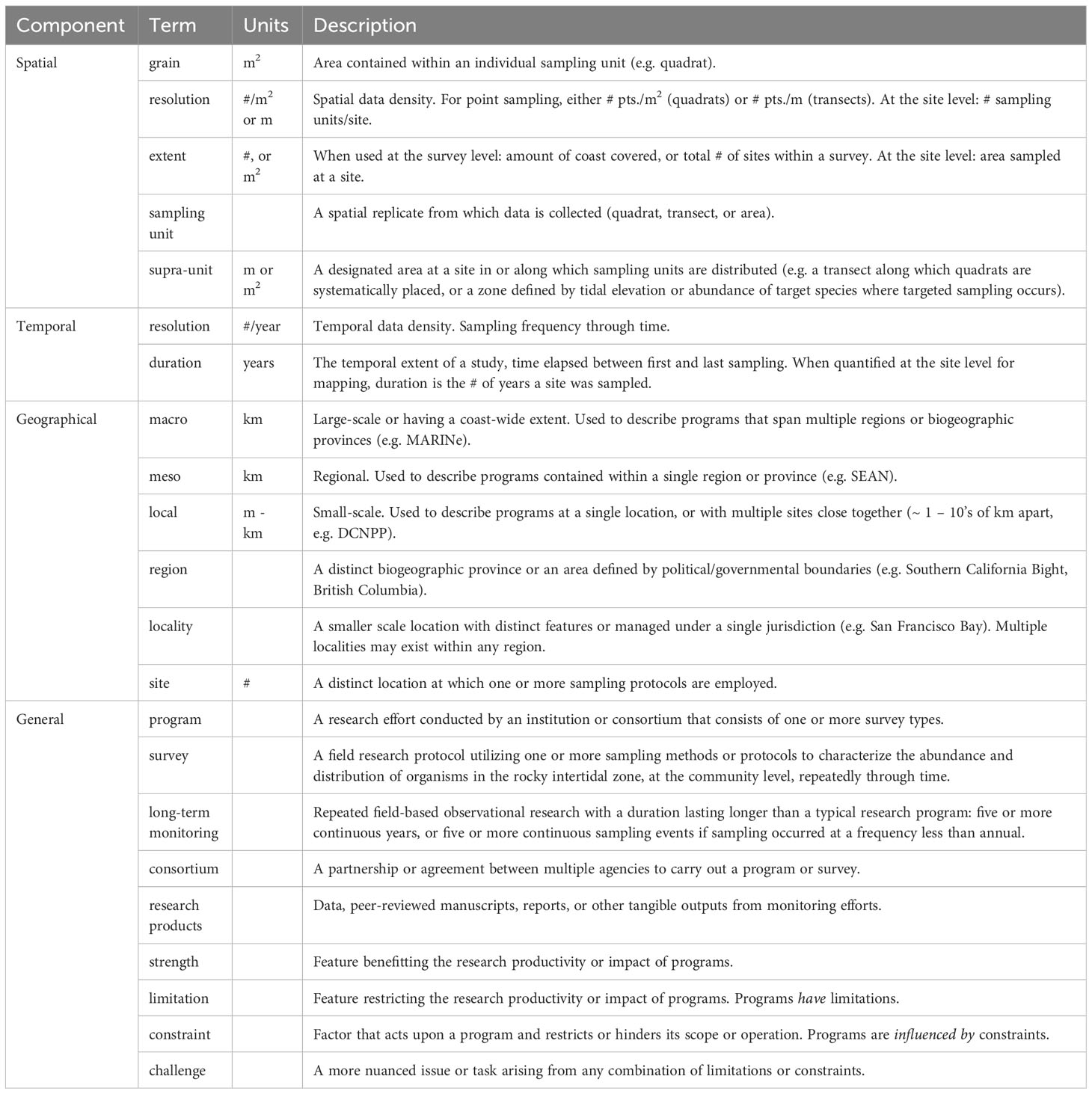
Table 1 Definitions for terms used within this review.

The rocky intertidal zone is one of the most extensively studied ecosystems and a source of influential research in population and community ecology (e.g. Ricketts and Calvin, 1939; Connell, 1961; Lewis, 1964; Dayton, 1971; Connell, 1972; Paine, 1974; Paine and Levin, 1981, to name a few). Compact variation in community structure at small spatial scales, high biodiversity, and primarily small, sessile organisms make the rocky intertidal zone amenable to ecological studies (Murray et al., 2006). Paradoxically, these and other features also make the rocky intertidal zone challenging to study. High temporal and spatial variation require labor-intensive in-situ surveys that are both expansive and highly resolved for accurate community characterization (Hartnoll and Hawkins, 1980; Hawkins and Hartnoll, 1983; Underwood and Chapman, 1996). High biodiversity requires advanced taxonomic expertise. Difficulty of access and a sampling window restricted to periods of emersion limit the area over which data can be collected at any site (i.e. 10’s to 100’s of m², Murray et al., 2006; Godet et al., 2009). Although recent remote sensing approaches permit data collection on larger spatial scales (i.e. 100’s to 1000’s of m²), technological limitations restrict their resolution and deployment, so in-situ field sampling remains the industry standard (Godet et al., 2009; Garza, 2019). Despite the availability of sampling design guidelines (see Murray et al., 2006 for an extensive treatment of the subject), the majority of studies in the rocky intertidal zone may suffer from poor or inadequate sampling design (Andrew and Mapstone, 1987; Underwood, 1991; Miller and Ambrose, 2000; Underwood et al., 2000). Therefore, monitoring of the rocky intertidal zone is emblematic of efforts in other marine systems; despite the strong history of work in this field, there remains a need to describe and find solutions to challenges inherent to LTM.

The Northeast Pacific Coast (NPC) provides an ideal case study for examining the scope, scale, and evolution of LTM of rocky intertidal ecosystems because surveys vary greatly in temporal duration, spatial extent, and sampling design. Some of the longest-term (multi-decadal) and largest scale (1000’s of km) observational studies of the rocky intertidal zone in the world have been conducted on the NPC, as well as some of the most temporally and spatially resolved (e.g. Steinbeck et al., 2005; Raimondi et al., 2019b). Monitoring has occurred in some cases since the 1930’s, a timeframe in which anthropogenic impacts on this system have increased significantly (Halpern et al., 2009). This work covers multiple biogeographic regions and includes both heavily urbanized and pristine coastlines (Schoch et al., 2006; Blanchette et al., 2008; Fenberg et al., 2015; Menge et al., 2015). These studies are comparable in duration and extent to long-term, large-scale monitoring programs in other temperate rocky intertidal systems around the world, such as those in the United Kingdom, South Africa, Chile, and Japan (Hartnoll and Hawkins, 1980; Dye, 1998; Navarrete et al., 2010; Mieszkowska et al., 2014; Ishida et al., 2021), and programs spanning multiple systems (Miloslavich et al., 2011; Cruz-Motta et al., 2020; Montes et al., 2021). Finally, these programs demonstrate the costs and benefits of diverse approaches: from small-scale intensive studies at high taxonomic resolution to larger scale but taxonomically coarser biogeographic studies.

Reviewing the diverse approaches to LTM of the rocky intertidal zone of the NPC is timely, as the value of LTM has never been greater (Magurran et al., 2010; Lindenmayer et al., 2012; Miller et al., 2012; Mieszkowska et al., 2014; Lindenmayer et al., 2015; Hughes et al., 2017; Micheli et al., 2020). Examining the causes and consequences of these approaches provides valuable insight to LTM efforts in other marine ecosystems that face similar logistical challenges related to temporal and spatial scale of observation (Andrew and Mapstone, 1987; Levin, 1992; Estes et al., 2018). Field methods need to be able to efficiently produce data capable of addressing impacts from climate change and other anthropogenic stressors (Thompson et al., 2002; Helmuth et al., 2006; Schoch et al., 2006; Mieszkowska et al., 2014; Raimondi et al., 2019b; Reed et al., 2022). A thorough review of the field methods employed by LTM programs across the NPC is currently lacking, and understanding the status of this field is crucial to capitalizing on available resources and improving the data these programs will provide in the future.

The purpose of this manuscript is to review LTM programs in the rocky intertidal zone of the NPC to address the questions: 1) What LTM sampling designs have been used to characterize rocky intertidal community structure through time? 2) Do relationships exist between sampling design components, and what do the direction and strength of these relationships reveal about logistical constraints on the scale of monitoring? 3) What are the major strengths and limitations of LTM programs? and 4) What are the anticipated future directions of LTM on the NPC? To answer these questions, I compiled a list of LTM programs, reviewed relevant literature, and interviewed practitioners. From this effort I extracted quantitative survey design information to provide a thorough description of each of the LTM programs on the NPC. I then characterized trade-offs between sampling design elements for a subset of comparable surveys. Finally, I used qualitative data analysis to summarize interview transcripts, evaluate strengths and limitations of these programs, and provide recommendations for best practices moving forward.

Materials and methods

Literature search and program list curation

I produced a list of LTM programs on the NPC to review through literature searches and direct contact of researchers at academic institutions (Supplementary Table 1). I define a program as a research effort consisting of one or more surveys conducted by an institution or consortium. I define a survey as a field research protocol utilizing one or more sampling methods to characterize the abundance and distribution of organisms in the rocky intertidal zone, at the community level, repeatedly through time (Table 1). First, I found program names by searching the Google Scholar and ISI Web of Science databases using the term “rocky intertidal long-term monitoring”. I then used reference and forward searches of all potentially relevant literature until doing so no longer produced new programs. Then I searched the name of each identified program directly in both databases to gather relevant literature.

Ultimately, I included a program in this review if certain criteria were met. First, the program had to conduct surveys that qualified as “long-term monitoring” (sensu Lindenmayer and Likens, 2010; Mieszkowska et al., 2014, see Table 1 for definition). Second, all necessary descriptive data on sampling design had to be obtainable from written descriptions of field methods (N = 1, Southeast Alaska Network (SEAN)), or a combination of literature and interviews (N = 17). The Multi-Agency Rocky Intertidal Network (MARINe) is a consortium of multiple agencies that adopted and employs standardized protocols. In instances where agencies within the MARINe consortium had preexisting, supplemental, or modified surveys in addition to the standardized MARINe protocols, I treated those agencies as distinct programs (North Coast and Cascades Network (NCCN), San Francisco Bay Area Inventory and Monitoring Network (SFAN), Greater Farallones National Marine Sanctuary (GFNMS), and the Mediterranean Coast Inventory and Monitoring Network (MEDN)).

In total I reviewed 18 LTM programs with 37 surveys. I collated sampling design data for each program and their surveys into two tables. Program-level data (e.g. agencies, program duration, regions) are provided in Supplementary Table 1. Survey-level data (e.g. inception and duration of each survey, number of survey sites) and information on how data are collected at survey sites (e.g. choice and distribution of sampling units) and within sampling units (e.g. metric recorded, grain, point sampling density) are provided in Supplementary Table 2.

Literature review

I gathered relevant primary literature and reports in three categories related to each program: 1) standard operating protocols (SOPs) or other descriptions of sampling design, 2) power analyses or other statistical analyses of sampling design, and 3) publications containing qualitative commentary on the strengths and/or limitations of programs (Supplementary Table 3). I extracted sampling design data from the literature related to each program to address questions 1 and 2. I also extracted strengths, limitations, constraints, challenges, and solutions, as well as future directions, to guide interviews and address questions 3-4.

Interviews

In some instances, the literature provided incomplete or outdated sampling design data. I utilized semi-structured interviews and qualitative data analysis to fill data gaps, verify design details, and gather information on goals, trade-offs, strengths and limitations, and future directions of programs. I contacted researchers across the NPC to determine whether a program existed at their institutions. During initial contact, I provided researchers with the overarching questions of this study, and asked if they had designed or conducted community-level long-term rocky intertidal monitoring and whether they would be willing to participate in an interview. When I did not find a description of study design during the literature review, I requested this information from practitioners during initial contact and reviewed these prior to interviews. All practitioners contacted agreed to an interview, but interview requests to the SEAN were not answered.

I conducted 25 semi-structured two-part interviews guided by a standardized questionnaire totaling 20.32 hours of interview time between 2020/11/05 and 2021/07/27 (Supplementary Material 1, Supplementary Table 3). I began interviews by briefly restating the goals of this study and then asking the interviewee to provide a general overview of their monitoring program. I then asked researchers to provide program and sampling design details (questions 1-2) and to evaluate program strengths, limitations, constraints, challenges, solutions, (question 3) and future directions (question 4). During each interview, I populated the questionnaire with notes on interviewee responses. At the end of each interview, I asked researchers to provide literature related to their program within each of the three categories discussed above. I used Transcribe by Wreally software to transcribe interview audio to text, then reviewed all text files and manually corrected transcription errors. The aspects of this study involving human participants were reviewed and approved by The UC Santa Cruz Office of Research Compliance Administration. Participants provided informed consent to participate in this study. Additionally, this study meets criteria for exemption described in 45 CFR 46.104 and/or the UC Santa Cruz Policy on Institutional Review Board Regulatory Flexibility.

Sampling design components

To address question 1, I analyzed quantitative data from my literature review and interviews. To visualize the temporal duration and spatial extent of programs, I collected sampling duration and coordinates for sites across programs and mapped them (Figures 1, 2). I also produced histograms of program duration and extent (Figure 3). To compare temporal and spatial data assets across regions, I calculated the maximum and mean site sampling duration and number of sites for each region (Table 2). Because surveys differ in metrics, sampling units, and taxa targeted, I described sampling design details (sampling units, grain, replication, distribution, and resolution) for those surveys that characterize benthic percent cover at the community level, in-situ, using quadrats or transects (31 of 37 surveys, Supplementary Table 4, for examples see Figures 4, 5). This effectively removed image-based surveys. A claim in the literature is that choice of sampling units is often made without explicit consideration of the size of organisms to be sampled (Kareiva, 1988; Levin, 1988; Wiens, 1989; Levin, 1992). To evaluate whether this holds true, I calculated the proportion of surveys using supplemental sampling units to sample taxa of interest, and compared the grain of supplemental units to that of sampling units used to collect community-level data (Supplementary Table 5). I conducted all qualitative and quantitative data analyses using R (R Core Team, 2021). Maps were created using the “maps” Package in R (Becker et al., 2021).

FIGURE 1

Figure 1 Map of LTM study sites across the NPC. Diameter of circles is scaled based on duration (number of years of data collected, range = 1 – 52 years) of each site.

FIGURE 2

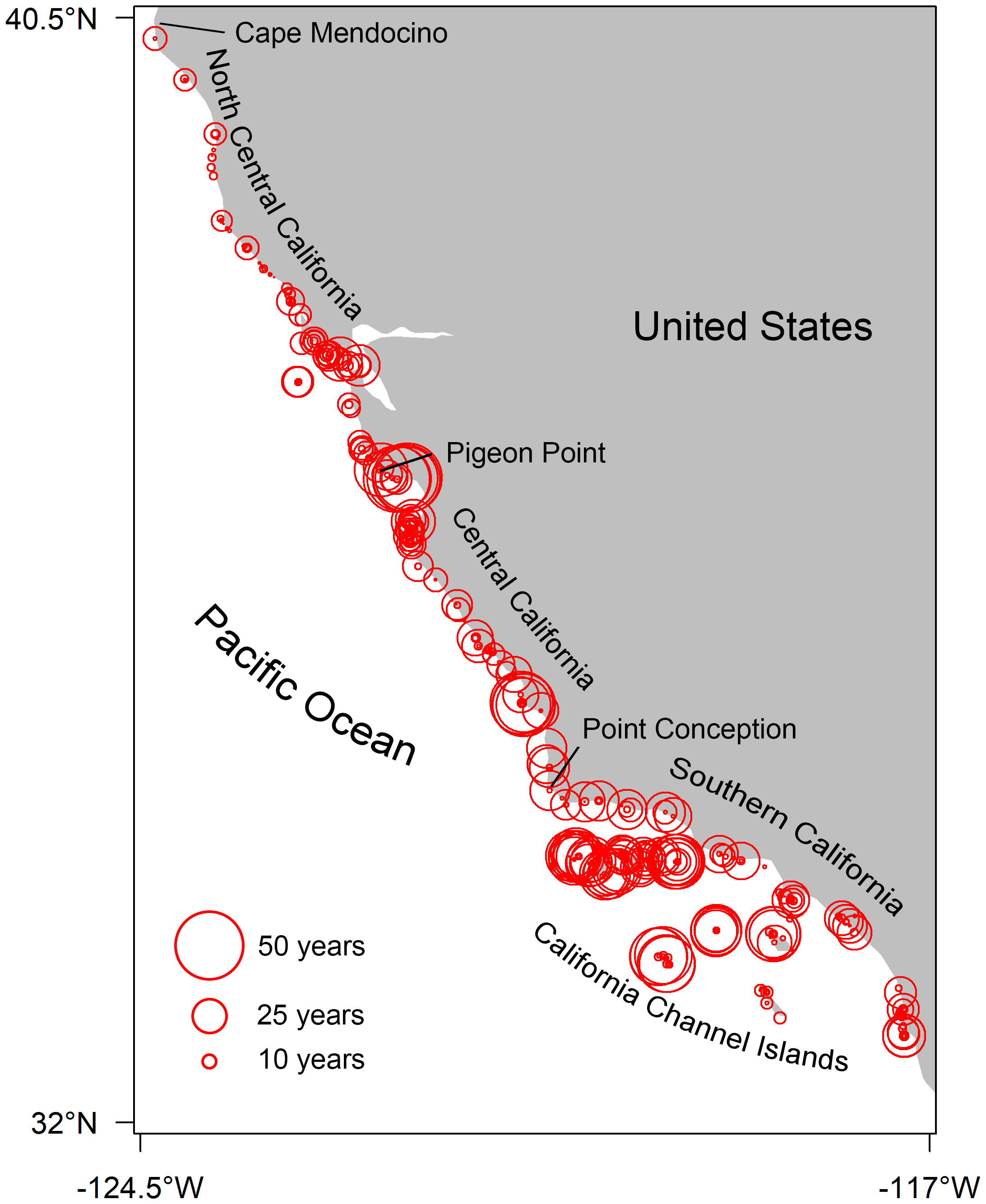
Figure 2 Map of LTM study sites within the most densely sampled regions (North Central to Southern California). Diameter of circles is scaled based on duration (number of years of data collected, range = 1 – 52 years) of each site.

FIGURE 3

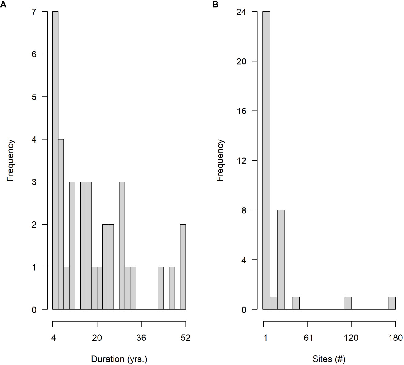
Figure 3 Temporal and spatial extent frequency distributions showing duration of surveys (A), and number of sites within a survey (B). Duration is grouped into bins with a width of 2, and number of sites is grouped into bins with a width of 10.

TABLE 2

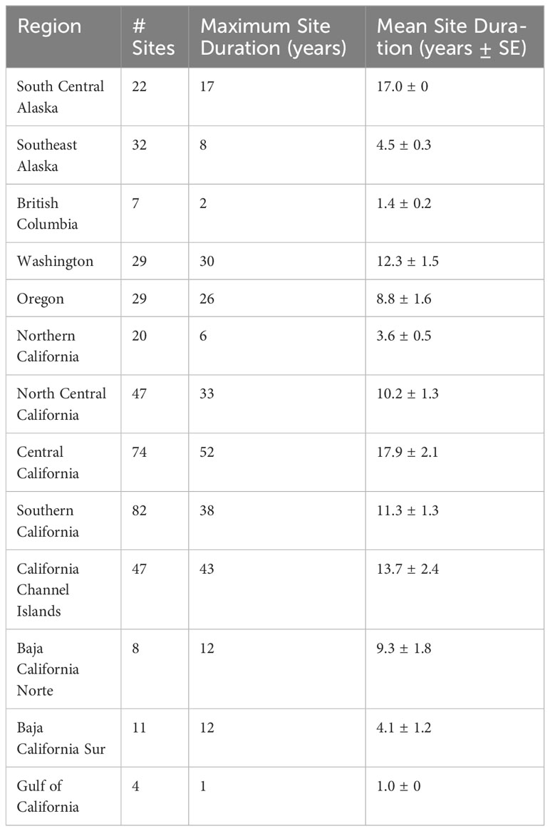
Table 2 Summary of data assets by region, listed from north to south.

FIGURE 4

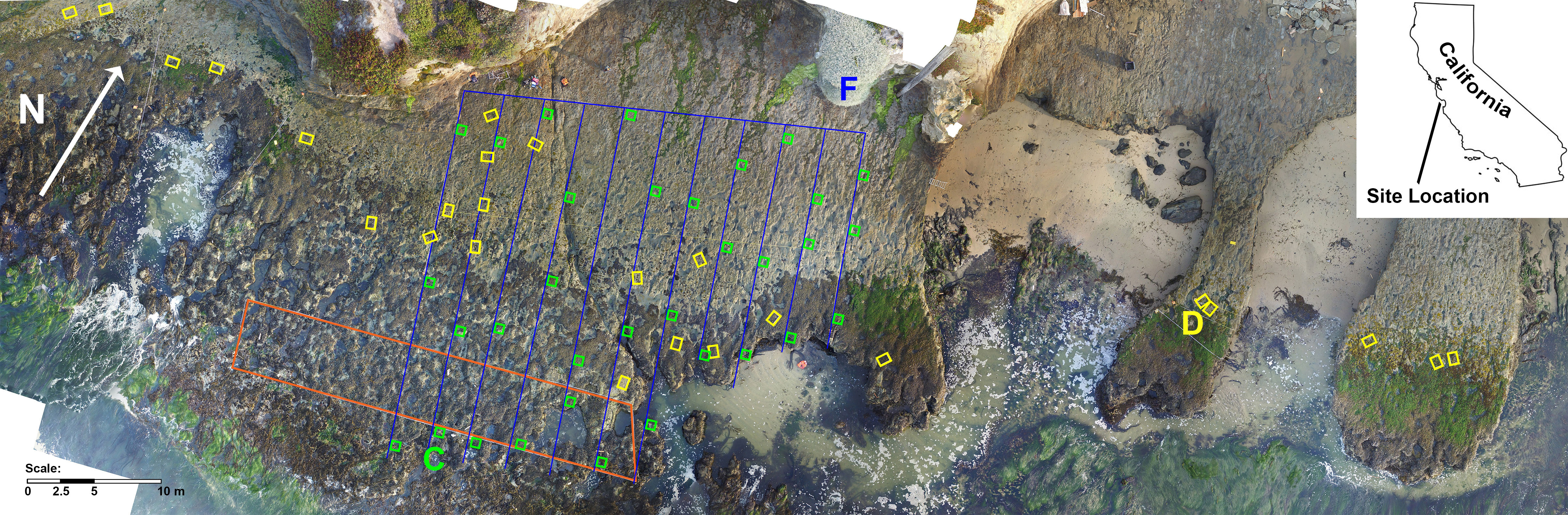
Figure 4 Example of sampling methods used to characterize a rocky intertidal study site (MARINe site Terrace Point, Santa Cruz, CA, USA). Site map annotated to show location of sampling units used in MARINe surveys. Fixed LTM Survey quadrats (D, yellow rectangles, 50 x 75 cm, grain = 0.375 m²) are used to estimate percent cover of target species at a replication of 5/species, covering a total of 1.875 m²/species/site at a sampling resolution of 267 points/m². A mobile invertebrate swath (orange trapezoid) covering ~ 575 m² is used to estimate abundance and size structure of Pisaster ochraceous as part of the LTM Survey. The Biodiversity Survey grid (F, blue lines) is used to estimate percent cover, and consists of 11 cross-shore point contact transects with a total combined transect length of 264.17 m and a sampling resolution of 10 points/m. In the Biodiversity Survey counts of mobile invertebrates are made in quadrats (C, green squares, 50 x 50 cm, grain = 0.25 m²) randomly placed adjacent to the transects, with a replication of 3/transect, or 33/site, covering a total of 8.25 m². In addition, counts of larger invertebrates (e.g. sea stars, abalone) are conducted in 2 m wide swaths along each of the cross-shore Biodiversity transects. Letter labels referenced match the label column in Supplementary Table 4 and the letter labels in Figure 5. UAV imagery collected by P. Robinson, UCSC. Orthophotomosaic produced by N. Kaplanis.

FIGURE 5

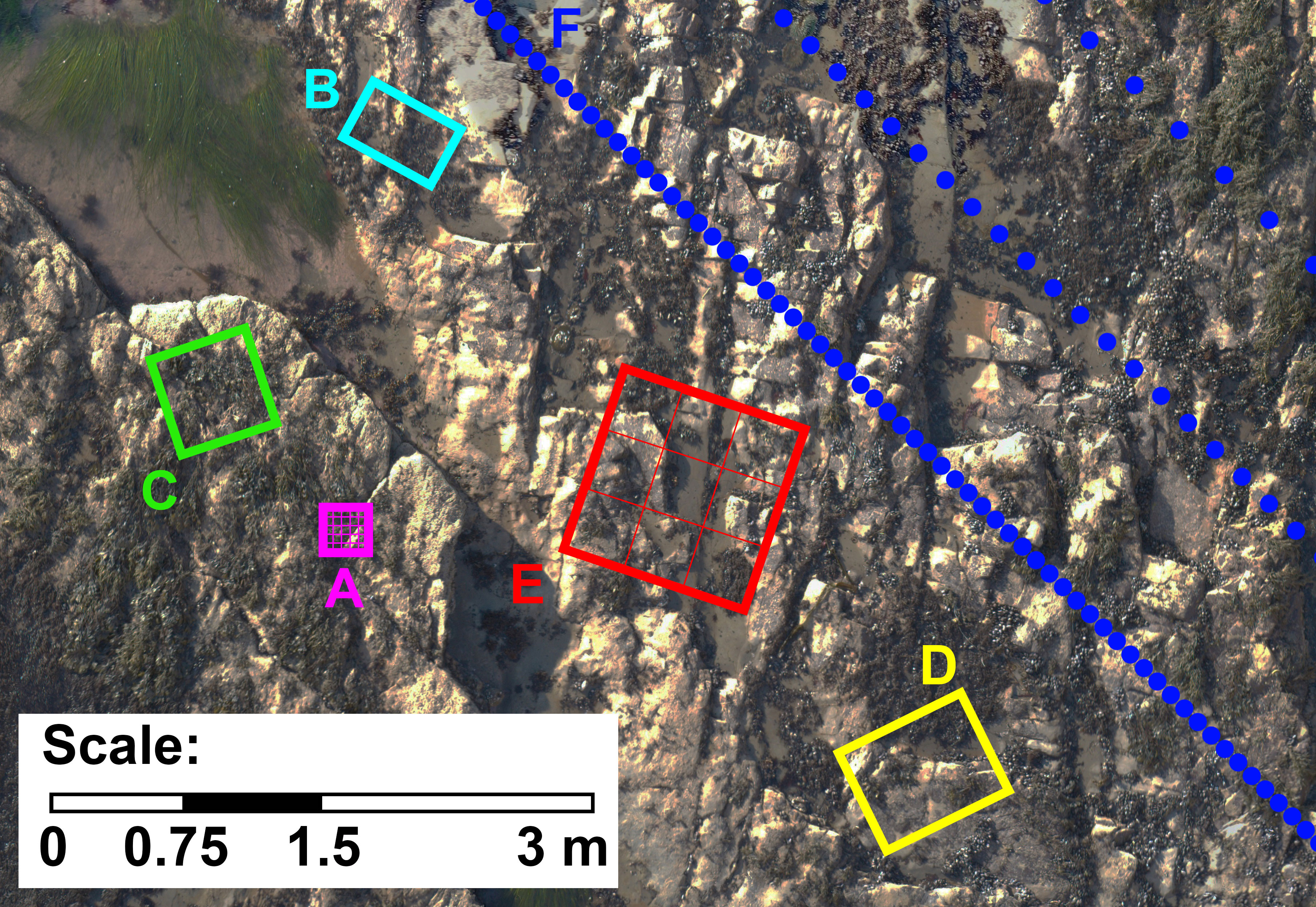
Figure 5 Commonly used quadrats and point intercept transects for in-situ characterization of benthic percent cover. Quadrats and transects are color coded and labeled with letters to match those in described and labeled in Figure 4 and Supplementary Table 4. The highest and lowest resolution point sampling quadrats used are depicted in magenta (A) and red (E).

Design trade-offs

To address question 2, I used correlation analysis to test whether relationships between pairs of design features exist, and to describe the direction and strength of these relationships. In this analysis, one survey from Catalina (CATA) and one survey from the Southern California Bight Baseline Study (SCBBS) were dropped from the 31 described above, the former because of missing descriptive data, and the later because this program employed an exceptional number of personnel to conduct simultaneous destructive sampling and experimental manipulations at monitoring sites, making it an outlier unsuitable for comparisons of labor. I tested whether correlations directionally and quantitatively match those expected under the assumption that resource limitation creates trade-offs between design components. Although access to resources (e.g. funding, personnel, equipment) likely varies across surveys and through time within surveys, quantitative data on resources was not available. I made comparisons that have been discussed in-detail in the literature (Andrew and Mapstone, 1987; Wiens, 1989; Levin, 1992; Murray et al., 2001; Estes et al., 2018). When deviations from expected relationships occurred, or relationships were found to be non-significant, then stand-out attributes of programs or approaches were assessed as potential explanations. For example, if a program was an outlier in some attribute or employed a unique solution to a logistical constraint, then this was explored as a potential logical explanation for the relationship found.

In the “Survey level” subsection, I made pairwise comparisons to evaluate whether limited resources create trade-offs between aspects of the breadth and resolution of surveys (Figure 6; Table 3). Specifically, I hypothesized that duration would be negatively correlated with number of sites and labor/survey (calculated as the number of personnel needed to sample one site x the number of low tides needed to sample one site x temporal sampling resolution (number of site visits per year) x number of sites in the survey), and that number of sites would be negatively correlated with sampling resolution and labor/site (calculated as personnel x tides). In the “Site and sampling unit level” subsection, these surveys were further filtered to include only those using quadrats (21 surveys). I made pairwise comparisons to evaluate whether limited resources create trade-offs between aspects of the breadth and resolution of data collection at sites and in sampling units (Figure 7; Table 3). Specifically, I hypothesized that area would be positively correlated with grain and replication and negatively correlated with resolution, resolution would be negatively correlated with grain, points/site would be positively correlated with replication and resolution, and replication would be negatively correlated with grain, points/quadrat, and resolution.

FIGURE 6

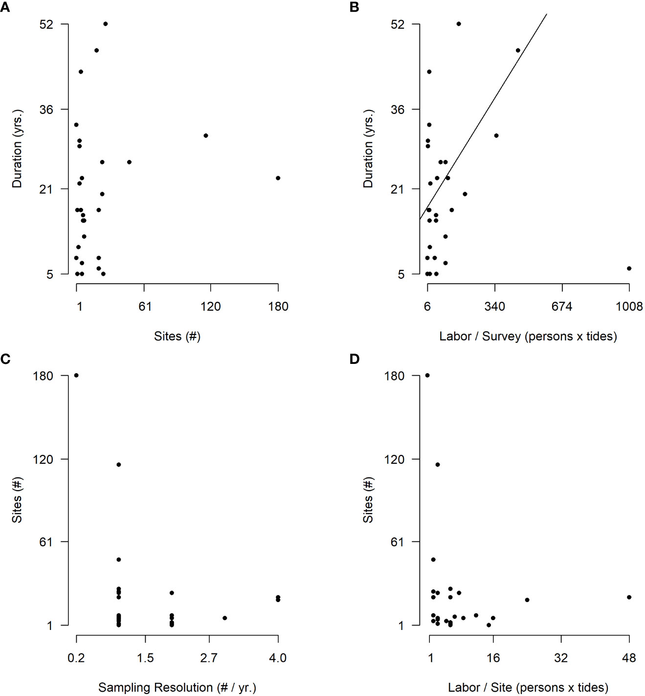
Figure 6 Survey-level sampling design trade-offs. Panels (A–D) examine emergent trade-offs between various design components of surveys and their temporal and spatial extents. Labor/site is presented as the number of personnel needed to sample a site x the number of tides needed to sample a site. Labor/survey is labor/site x temporal sampling resolution (number of visits/year) x the number of sites in the survey.

TABLE 3

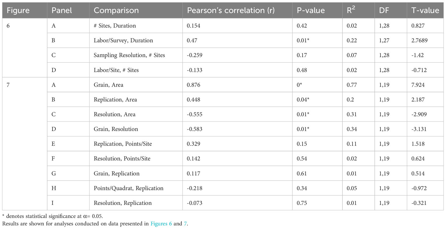
Table 3 Summary statistics for correlation analysis of sampling design components.

FIGURE 7

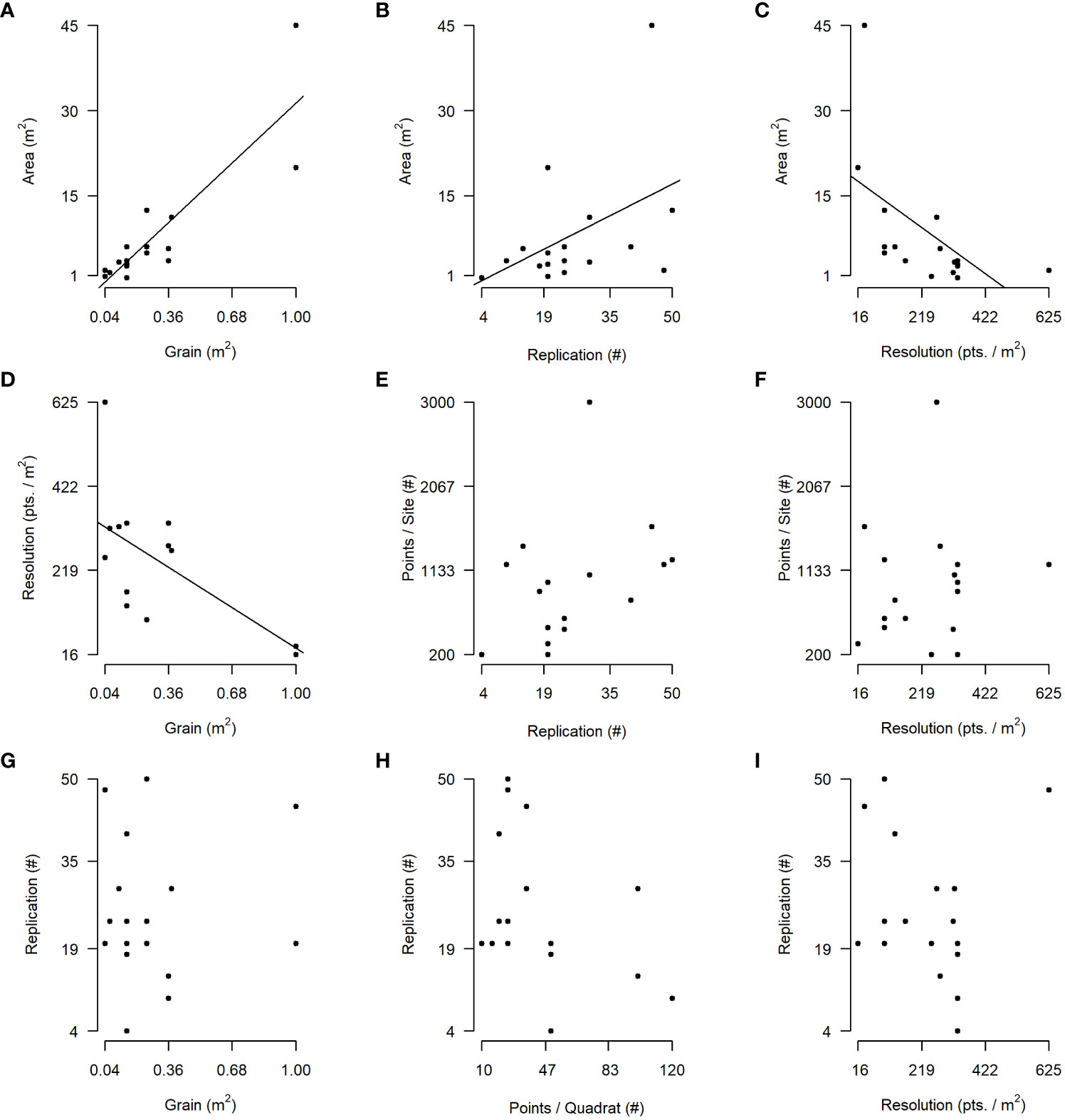
Figure 7 Sampling unit-level design trade-offs. Panels (A–I) examine trade-offs between various design components of in-situ quadrat sampling to characterize benthic percent cover.

Strengths, limitations, constraints, challenges, and solutions

To address questions 3 and 4, I used qualitative analysis of interview data to summarize the knowledge of the practitioners of this work. I used the package RQDA to code transcripts and conduct a systematic, deductive, qualitative analysis (Huang, 2016; Chandra and Shang, 2019). I developed a codebook containing categories derived from major themes in the interview questionnaire, category definitions, codes, and code definitions (Supplementary Table 6). Codes were based on a-priori knowledge of interview topics and this field of study. I reviewed interview transcripts and tagged clauses with first-order codes. After coding transcripts, I grouped codes into second-order concepts, dropping unused codes, combining similar codes, and refining codes to match the actual language of the interview content. This coding allowed data query and subsequent analysis. To evaluate the prevalence of goals, factors dictating site distribution and characterization, and overall program strengths, limitations, and constraints, I produced and ranked the percentages of respondents using codes (Supplementary Table 7). I also calculated and ranked the percentages of interview respondents citing major challenges, both with and without proposed solutions (Supplementary Table 8). To distinguish between these concepts, I define a limitation as a feature restricting the research productivity or impact of a program, and a constraint as a factor that acts upon a program and restricts or hinders its scope or operation. Here programs have limitations and are influenced by constraints. I define a challenge as a more nuanced issue or task arising from any combination of limitations or constraints (Table 1). Strengths are discussed in contrast to limitations, whereas solutions are discussed as being devised to address challenges.

Direction of the field

I extracted practitioner opinions of research priorities and desired program improvements from interviews as potential future directions of programs (Supplementary Table 8). Whenever a practitioner indicated either that they would like to address a research question using program data but had not yet done so, or that they would like to address a research question but program data were not yet capable of addressing it, I recorded that research question as a future direction. Because image-based sampling is an emerging frontier within this field, I also compared the strengths and limitations of these approaches to traditional in-situ sampling to provide a sense of how they may be used in future monitoring.

Results

Literature review

I found that 31 surveys (84%) have documentation providing some level of sampling design information, but that only 19 surveys (51%) have a formal SOP. Only 14 surveys (38%) have a published power analysis or other statistical evaluation of their sampling design. I found 18 publications with commentary on strengths and/or limitations of sampling design (Supplementary Table 3).

Sampling design components

Program goals

Every program reviewed had multiple goals. The most common program goals cited by interview respondents were: documenting changes in biological communities through time (70% of respondents), providing data for impact assessment (primarily oil spills, 65%), and gathering baseline information (61%). Following these gathering data to understand climate change impacts (30%) and informing policy or management (22%) were commonly cited goals. In contrast, providing education was cited by only 13% of respondents, and documenting spatial variation was cited by only 9% of respondents (Supplementary Table 7).

Temporal duration and sampling resolution, spatial extent, site selection

Programs range in duration from 5 - 92 years. The earliest program began in 1931 and the most recently initiated program began in 2016 (Supplementary Table 1). Surveys range from 5 - 52 years of continuous sampling. Median survey duration is 18.5 years, and eight surveys have 10 years of data or less (Figure 3A). Survey sampling resolution ranges from 0.2 - 24 surveys/year. The most common sampling resolution is annual (22 surveys), then semiannual (10 surveys). North Central California to Alaska are mostly sampled in the Summer, while regions south of this are sampled across all seasons, corresponding with the timing of daylight low tides. Most in-situ surveys (27/31) are conducted at a rate of 1 low tide/site but range from 1 - 5 low tides/site.

Programs include over 600 sites distributed across approximately 34° of latitude and 42° of longitude from Punta Abreojos, Baja California Sur, México, to the Katmai Peninsula, Alaska, United States of America (Figure 1). Surveys have a wide range of sites (1 – 180) and 18 sites on average. Most surveys (25/37) have 10 or fewer sites, 10 surveys have between 11 and 50 sites, and two have more than 100 (MARINe Long-term Monitoring and Biodiversity Surveys, 116 and 180 sites respectively, Figure 3B; Supplementary Table 2).

The most common site attributes considered during site selection were substrate type (cited by 48% of respondents), accessibility (43%), areas at risk of impacts (39%), historical research sites (35%), and areas with target species (35%). Equal proportions of respondents (30%) said sites were selected to cover a region (e.g. Southern California, Prince William Sound), a jurisdiction (e.g. Kenai Fjords, Katmai, Olympic, Redwood, and Channel Islands National Parks), and according to funding. Only 13% of respondents said a geospatial sampling scheme (i.e. hierarchical or random distribution) was used during site selection (Supplementary Table 7).

Site distribution is spatially patchy, and regions also have variable temporal data coverage. The regions of Southern, Central, and North Central California, and the Channel Islands have far more sites than other regions, despite their relatively short coastlines. In addition, these regions have longer histories of research (Figure 2; Table 2). For example, Southern California has 82 unique sites where monitoring has been conducted, a maximum site duration of 38 years and a mean duration of 11.3 ± 1.3 (SE) years of data per site. In contrast, despite having extensive rocky intertidal coastline, Southeast Alaska, British Columbia, and Baja California Norte and Sur, have few study sites and short research durations(Table 2). Baja California Norte, for example, has only 8 sites, a maximum site duration of 12 years, and a mean site duration of 9.3 ± 1.8 (SE) years of data per site. Overall, there are large discrepancies in data assets across regions (Table 2).

Sampling units, grain, replication, distribution, and resolution

I found that 15 programs use quadrat sampling in 21 surveys, and 7 programs use point intercept transects in 10 surveys (Supplementary Table 4). Of the surveys using quadrats, 15 use point sampling, and 6 use visual estimates of percent cover. Of the surveys using point sampling in either quadrats or transects, 20 sample additional layers beyond first contact. The most common rules for determining how many additional layers to sample are: up to 3 layers, until the primary substrate is reached, and up to 2 layers.

Quadrats range from 0.2 x 0.2 m (0.04 m²) to 1.0 x 1.0 m (1.0 m²) and the most common quadrat sizes used (each in 5 surveys) are 0.5 x 0.75 m (0.375 m²) and 0.3 x 0.5 m (0.15 m²). Of the 21 surveys using quadrats, almost all (19/21) use quadrats smaller than 1.0 m². Of the 10 surveys using point intercept transects, half use 10 m long transects, while the other half use transects of variable lengths. Site-level replication of quadrats ranges from 4 - 50 replicates/site, and the mean is 24 replicates/site ± 3 (SE). Replication is also variable within grain (e.g. 0.15 m²: range = 4 – 40 replicates/site, 0.25 m²: range = 20 – 50 replicates/site). Site-level replication of transects ranges from 3 - 11 replicates/site, and the mean is 8 replicates/site ± 2 (SE). For quadrat surveys, total area sampled/site ranges from 0.6 m² - 45.0 m² and total number of points sampled/site ranges from 200 to 3000. For surveys using transects with fixed lengths and number of points sampled, length sampled/site ranges from 30 - 300 m, and total points sampled/site ranges from 330 – 1500. Point sampling resolution in quadrats ranges from 16 to 625 pts./m², and the mean is 193 pts./m² ± 29 (SE). Point sampling resolution in transects ranges from 3 - 10 pts./m and the mean is 6 pts./m ± 1 (SE). Most surveys use uniform point sampling (27/31). Random point sampling is used in only 4 surveys (3 within quadrats and 1 survey on transects). Fixed sampling units are used in 19 surveys, units that are randomly distributed for each sampling event are used in 10 surveys, and both fixed and random units are used in 2 surveys (Supplementary Table 4). Mean replication in surveys using fixed units is 18.4 ± 2.4 (SE), while mean replication in surveys using random units is greater at 28.7 ± 4.8 (SE).

Supplemental sampling units and parameters

Most (12/18) programs supplement their community-level sampling with taxon specific sampling using grain catered to the size of the organisms sampled (Supplementary Tables 2, 5). Of all programs, 7 sample larger units for larger taxa, 1 samples smaller units for smaller taxa, and 4 use both smaller and larger units for smaller and larger taxa. Taxa commonly targeted with supplemental sampling units include abalone (Haliotis spp.), anemones (Anthopleura spp.), barnacles (Chthamalus dalli, Balanus glandula), chitons (Katharina tunicata, Cryptochiton stelleri), limpets (Lottia persona, Lottia gigantea), sea stars (Pisaster ochraceus, Evasterias troschelii), and snails (Nucella spp., Littorina spp.). In all instances, counts or timed searches are used to enumerate target species rather than point sampling.

Design trade-offs

Survey level

In comparing aspects of sampling design at the survey level I found one statistically significant correlation (Figure 6; Table 3). Labor/survey is positively correlated with survey duration. (Figure 6B). I found no significant correlations between the number of sites in a survey and survey duration, temporal sampling resolution, nor labor/site (Figures 6A, C, D).

Site and sampling unit levels

At the site and sampling unit levels I found four statistically significant trade-offs between design components (Figures 7A–D; Table 3). Area sampled/site is significantly positively correlated with grain and replication but is significantly negatively correlated with sampling resolution (Figures 7A–C; Table 3). I also found a significant negative correlation between point sampling resolution and grain (Figure 7D; Table 3). I found no significant correlations between total number of points sampled/site and replication nor resolution (Figures 7E, F; Table 3). Finally, I also found no significant relationship between replication and grain, points/quadrat, nor resolution (Figures 7G–I; Table 3).

Image-based approaches

Some programs use image-based sampling approaches to characterize sites, rather than traditional in-situ plot-based sampling, and in some cases have achieved sampling that is more extensive, intensive, or efficient. For example, SCBBS has 1 technician sample 20 pts./quadrat in-situ and 2 technicians each sample 154 pts./quadrat from images in the lab, representing a 15-fold increase in data resolution between the in-situ and lab sampling. The Tribal Intertidal Digital Ecological Survey (TIDES) creates orthophotomosaics of 180 m² plots at each study site and digitally samples these using 9600 stratified random points (53 pts./m² point sampling resolution). Thus, this project samples 4 times the area/site of the most extensive in-situ quadrat sampling, at greater resolution than two in-situ quadrat surveys. The Universidad Autónoma de Baja California (UABC) conducts in-situ surveys and digital imaging surveys using an UAV at the same sites, but surveys 2 times/year in-situ and 24 times/year via UAV. By transitioning from quadrat sampling to UAV surveys the CATA program has decreased time required to sample each site from multiple low tides to 90 minutes, and their field teams have decreased from 4-5 to 2 people.

Strengths, limitations, constraints, challenges, and solutions

Interviews revealed common strengths and limitations (Supplementary Tables 7, 8). The most cited strength was refining or improving methods through time (83% of respondents). After this, respondents said their programs had particularly valuable or strong data features (e.g. taxonomic resolution or consistency, 43%), produced good quality products or a good quantity of products (such as data or manuscripts, 43%), and did a good job of collaborating with others (39%). Finally, 30% of respondents expressed ease of data collection and data consistency as program strengths. Conversely, 43% of respondents said their program produced limited or insufficient products. For temporal duration and spatial extent, 30% and 39% of respondents said their program was strong, but 39% also said that their program had a limited scale of inference. More specifically 9% said that their program was limited in temporal duration, and 22% said it was limited in spatial extent. Another major limitation cited was data gaps, both temporal and spatial (22%). These data gaps are caused both by missed sampling opportunities and by sampling design, and range in scale from gaps at the site level to the program level.

Most practitioners cited funding (65%) and basic logistical challenges (such as the challenge of accessing sites and the labor-intensive nature of sampling intertidal areas, 57%) as constraints. Following these, maintaining a team of trained personnel with sufficient expertise (specifically taxonomic expertise and publishing capacity, 57%) was a commonly cited constraint (Supplementary Table 7).

Interviews also revealed common challenges with solutions found within or across programs (Supplementary Table 8). Twenty eight percent of respondents acknowledged the contrasting benefits of maintaining consistent sampling methods and refining methods to increase efficiency or to allow resources to be diverted to collecting other data. Programs that have addressed this issue did so through statistically evaluating methods to determine power to detect various levels of change or address questions, and dropping or adjusting protocols deemed insufficient, even if they had been carried out for extended periods of time. An equal proportion of respondents (28%) discussed the challenge of maintaining consistency in taxonomic identifications through time and across groups. This has been addressed through having consistent data collectors through time, maintaining updated databases, and developing and sharing consistent standards for taxonomic identifications. Although the benefit of saving time in the field with image-based sampling protocols was discussed by respondents, 20% of respondents also acknowledged that processing (storing, scoring etc.) photographic time series is a challenge. Cloud-based and automated image processing and storage were proposed as solutions.

Direction of the field

When asked about the future of their programs the most highly cited goal (48% of respondents) was to collect supplemental data (such as physical or environmental data). Additional future goals were to: utilize program data to produce more publications (26%), train new personnel or increase expertise among program team members (22%) and implement new sampling technology (e.g. image-based approaches, environmental sensors, 22%) (Supplementary Table 7).

The most cited remaining challenge was utilizing program data to produce publications or other data products (discussed by 52% of respondents, Supplementary Table 8). Those who cited this issue explained that limited funds force them to focus on data collection, which can hinder hiring and continuing to employ personnel with the motivation and expertise to analyze program data and produce publications. Developing taxonomic expertise was the next most cited challenge (28% of respondents). This was cited as an ongoing concern, especially in the context of personnel turnover due to the long-term nature of these studies. In terms of site characterization, the long-standing debate over whether to use fixed or random sampling units is clearly an unresolved issue: 36% of respondents cited concerns over the use of fixed units (namely limited scale of inference and ability to extrapolate beyond units and lower replication due to time constraint of unit relocation), and 20% of respondents cited concerns over the use of random units (namely limited capacity to document changes through time due to high spatial variation).

Many respondents (43%) discussed questions that they would like to address but that remain unanswered (Supplementary Table 8). These questions revealed that much work remains on topics from programmatic efficiency (e.g., how to use technology and better collaborate) to applied research on climate change impacts (e.g., sea-level rise impacts, latitudinal shifts) to resource management (e.g., how to establish baselines and accurately document changes in community structure and function).

Discussion

This review describes the operation and status of LTM programs on the NPC. I summarized sampling design features and presented this information in an accessible format (Supplementary Tables 1, 2). I also gathered relevant literature into a single table, a previously lacking resource (Supplementary Table 3). I found that gaps exist in the literature describing this work, which required interviews to acquire descriptive data. Collating this data revealed that LTM on the NPC has occurred at unrivaled temporal durations and spatial extents. Still, the temporal resolution and spatial extent of data collection at sites remains somewhat limited. In addition, important regions remain understudied. These programs primarily use simple in-situ observational sampling approaches but are increasingly employing digital imaging techniques. I analyzed correlations between sampling design features to evaluate the direction and strength of trade-offs between them and found that basic logistical constraints continue to impact the scale of data collection efforts. Finally, I synthesized practitioner knowledge to provide strengths, limitations, constraints, challenges, and recommendations for the future of this field.

Literature review: major conclusions

Much has been written on LTM on the NPC, but some literature was challenging to access, and basic methods descriptions are lacking for some surveys. This is concerning because repeatability is key to rigorous LTM and limited methods description increases the risk of protocol drift, which can prevent comparison of data collected at different time points or by different groups (Murray et al., 2006; Gilbane et al., 2022). Clear and accessible SOPs enable different groups to collect comparable data over broader scales. In addition, lack of documentation of protocols and data descriptions can discourage those unfamiliar with surveys from using data. Interviews made clear this was of particular concern for legacy programs (e.g. Hopkins Marine Station (HMS) Interview 1, 2). Efforts to utilize historical baseline data are lacking (though see Barry et al., 1995; Smith et al., 2006; Bonsell, 2013; Fales and Smith, 2022). Past quantitative baselines (pre 1990’s for most locations) of the abundance and distribution of rocky intertidal taxa remain rare, even when data are available for taxa of general interest like mussels and abalone, and intensively studied regions like Southern California (HMS Interview 2, CATA Interview 2). Historical data are important for understanding ecological variability, as they extend the temporal frame of reference and allow for distinction of natural versus anthropogenic changes (Wolfe et al., 1987; Magurran et al., 2010; Mieszkowska et al., 2014; Hughes et al., 2017; Raimondi et al., 2019b; Micheli et al., 2020; Gilbane et al., 2022).

One of the most important components of any SOP that should be further prioritized is clear and accessible data management protocols (Dean et al., 2014; Gilbane et al., 2022). This review provided some valuable guidelines that can help ensure data can be efficiently quality checked, archived, and shared. It is critical to standardize data collection, entry, and storage protocols across all groups involved in a program (MARINe Interview 1,2). It is also necessary to develop a written document that summarizes these protocols and defines responsibilities for implementing them (Dean et al., 2014; Gilbane et al., 2022). Finally, it is crucial to develop rigorous contextual metadata that adheres to accepted content standards such as the Ecological Metadata Language (EML), and to publish this information so interested parties can understand program data (Fegraus et al., 2005; Michener, 2015; Jones et al., 2019). For example, MARINe made developing high quality metadata a core component of their workflow and publishes metadata for all protocols within the DataONE Catalog, an open access repository that includes software for metadata documentation. Few programs openly share their data, but open data access should be prioritized. One of the most promising solutions is to share data through existing collaborations and repositories such as the Global Biodiversity Information Facility (GBIF), the Global Ocean Observation System (GOOS), the Knowledge Network for Biocomplexity (KNB), the Marine Biodiversity Observation Network (MBON), or the Ocean Biodiversity Information System (OBIS) (Duffy et al., 2013; Michener, 2015; Benson et al., 2018; Canonico et al., 2019). Doing so allows data to be utilized by interested parties outside of the programs, increasing the temporal and spatial scale of inference (Duffy et al., 2013; Michener, 2015; Benson et al., 2018; Canonico et al., 2019; Heberling et al., 2021). Ultimately, programs with accessible SOP’s, websites, metadata, and databases are the most productive in terms of research products (e.g. Gulf Watch Alaska (GWA), MARINe, PISCO).

Only 38% of surveys have a published power analysis or other statistical evaluation of sampling design, even though the most cited program strength was regular re-evaluation of methods. It is generally understood that statistical evaluation and regular re-evaluation of sampling methods is important to maximize the efficiency of data collection efforts (Hinds, 1984; Gilbane et al., 2022). Studies that compare aspects of sampling design (Foster et al., 1991; Meese and Tomich, 1992; Dethier et al., 1993; Miller and Ambrose, 2000) and provide recommendations for carrying out LTM of the rocky intertidal zone (Hartnoll and Hawkins, 1980; Hawkins and Hartnoll, 1983; Steinbeck et al., 2005; Murray et al., 2006; Irvine and Shelly, 2013; Mieszkowska et al., 2014; Raimondi et al., 2019b; Gilbane et al., 2022) are available and can help ensure statistically sound sampling, increase sampling efficiency, and improve the prospect of long-term program sustainability. Still, power analysis and other statistical evaluation has not been prioritized by practitioners on the NPC (NCCN Interview 2, MARINe Interview 2). Conducting and publishing statistical analyses of existing sampling designs should be further prioritized to improve access to information on designing and refining rigorous LTM.

Sampling design components

Program goals

LTM data have been successfully used to document changes in abundance of multiple taxa through time (Bonsell, 2013; Wootton and Forester, 2013; Roletto et al., 2014; Bodkin et al., 2018). Programs have addressed the impacts of sea-star wasting disease (Miner et al., 2015; Konar et al., 2019), withering foot syndrome (Altstatt et al., 1996; Raimondi et al., 2002), point source thermal and nutrient pollution (Schiel et al., 2004; Steinbeck et al., 2005; Pearse et al., 2015), and oil spills (Raimondi et al., 2009; Raimondi et al., 2011; Raimondi et al., 2019a). Programs have published biogeographical descriptions that allow better understanding of baseline conditions (Schoch et al., 2006; Blanchette et al., 2008; Fenberg et al., 2015; Menge et al., 2015). Data have also been used for documenting large-scale changes in relation to a recent marine heatwave (Miner et al., 2021; Weitzman et al., 2021), as well as those potentially driven by long-term climate change (Barry et al., 1995; Micheli et al., 2020). Finally, LTM data have informed policy and management, specifically in the design and evaluation of both the Oregon and California marine protected area (MPA) networks (Blanchette et al., 2014; Craig et al., 2017; ODFW, 2022; Raimondi et al., 2022). Still, fulfilling some program goals remains challenging. Although documenting changes in biological communities is the most cited goal, most publications focus on individual taxa. Studies of change at the community level are rare (Miner et al., 2021) and many studies often use only a subset of data, and so remain limited in their taxonomic, spatial, and/or temporal scope. The use of data subsets in publications results from the challenge of maintaining consistent sampling across space and through time, which can render portions of datasets unusable (MARINe Interview 2). In addition, taxonomic inconsistencies across groups carrying out sampling at different locations or times can make data incompatible. LTM programs can ensure data compatibility through developing rigorous taxonomic identification and data collection guidelines, databases, and standard operating protocols (Gilbane et al., 2022).

Temporal duration and sampling resolution, spatial extent, site selection

These programs operate over a range of temporal and spatial scales, with some programs exceeding 50 years of continuous sampling data and having sites distributed across thousands of kilometers. It is clear though that achieving this sampling scale is rare, as few multidecadal studies provide data across regions. Maintaining funding for survey teams, sampling regimes, and databases was the most frequently cited constraint. Limited funding requires prioritizing data collection at specific locations at specific times, which impacts temporal duration, spatial scale, and temporal and spatial resolution (MARINe Interview 2, NCCN Interview 1, MEDN Interview 1-2). Programs on the NPC that have persisted for multiple decades and that sample across regions (GWA, MARINe, PISCO, LiMPETS) are valuable models for successful long-term, large-scale ecosystem monitoring.

The temporal and spatial variation inherent to rocky intertidal communities makes determining when and where to sample difficult (Lewis, 1964). Most programs sample annually, as collecting finer temporal resolution data is cost prohibitive in the long-term. This funding constraint paired with the difficulty of sampling multiple seasons – due to lack of daylight low tides, and adverse conditions (particularly at higher latitudes) – restricts capacity to document short term variability (PISCO Interview). Where to sample is still commonly determined by access – the most cited site selection consideration after the presence of rocky habitat. Access is restricted by private property and limited access points, and much rocky intertidal habitat is remote and difficult to travel to within the tide window. In addition, respondents cited that they must restrict sampling to within jurisdictional boundaries (e.g. National Parks, MARINe Interview 2, NCCN Interview, MEDN Interview). Limited access creates temporal data gaps when a site can only be accessed with great effort and thus infrequently (such as only during certain seasons), and spatially when a site cannot be accessed at all. The logistical challenge of access has driven major differences in the number of sites and temporal coverage across regions, which is especially apparent in Baja California, México and British Columbia, Canada (MARINe Interview 2, UABC Interview, Figure 1; Table 2). Sampling more sites in both Baja California and British Columbia will prove valuable for predicting and detecting distributional shifts, as the range edges of many species occur in these areas, and these coasts may also serve as refugia for future climate change driven shifts (Harley et al., 2006; Schoch et al., 2006; Pinsky et al., 2013).

Expanding inference beyond sampled sites is a common challenge to LTM, but programs on the NPC provide a range of solutions. The SEAN utilizes systematic sampling of a limited number of sites following shoreline geomorphological classification to allow extrapolation to areas with similar features (Irvine, 2010). This approach requires extensive coastal geomorphology data that is often lacking, and inference may still be limited to within regions (Schoch and Dethier, 1996; Schoch et al., 2006; Irvine and Shelly, 2013). The PISCO program uses a spatially nested site distribution scheme, where sampling is replicated hierarchically to allow comparison of communities across a range of scales (Schoch et al., 2006). Still, limited access and availability of rocky substrate prevented strict randomization of site locations (Schoch et al., 2006, PISCO Interview). Gulf Watch Alaska (GWA) employs a geospatial sampling scheme in which spatially balanced, randomly selected sites were selected within coastline designated as sheltered rocky habitat in a GIS database (Dean et al., 2014). Although this approach is statistically sound, inaccuracies in the shoreline classification database and the challenge of access required discarding or modifying some site locations (Dean et al., 2014). This sampling is made possible by accessing sites via boat along mostly sheltered coastlines, which is resource intensive and impractical on the open coast (GWA Interview 1,2, North Coast and Cascades Network (NCCN) Interview 1,2).

Sampling units, grain, replication, distribution, and resolution

Sampling designs vary across surveys despite sharing common goals. Design choices deserve consideration, as they can impact sampling efficiency and overall data quality, and design determines whether results can be compared across programs. Point intercept transects are used to characterize benthic percent cover half as commonly as quadrats despite multiple studies demonstrating that point intercept transects provide more accurate estimates of cover than simple random or optimally allocated stratified random quadrats (Miller and Ambrose, 2000; Murray et al., 2006), and provide greater power to detect temporal change (Irvine, 2010; Irvine and Shelly, 2013). In addition, point sampling is used more often than visual estimates despite evidence that visual estimates of benthic cover may be more precise and accurate, take less time to conduct, and better capture rare species (Dethier et al., 1993). The risk of error from subjective differences between observers using visual estimates may encourage the use of point sampling (Murray et al., 2006). The narrow range of grain for in-situ surveys that use quadrats could stem from sampling unit grain being largely motivated by practical considerations rather than by quantitative evaluation of the spatial scaling of the distribution of organisms (CATA Interview 2). Spatial scaling of the distribution of organisms is difficult to characterize, but is important and should be given more consideration when choosing sampling units (Kareiva, 1988; Wiens, 1989; Levin, 1992; Blakeway et al., 2003).

I found a range of replication, point sampling resolution, area sampled/site, and number of points sampled/site. This reveals that surveys conduct varying levels of sampling effort to collect the same metrics. It is worth considering how design choices impact survey efficiency, but few studies have quantitatively evaluated the consequences of varying grain, resolution, and replication of sampling units in the rocky intertidal zone (but see Miller and Ambrose, 2000). The range of effort across programs suggests that despite the availability of guidelines for how to determine the required level of sampling effort for any parameter of interest, design choices are ultimately determined by many factors other than desired levels of precision (Hartnoll and Hawkins, 1980; Hawkins and Hartnoll, 1983; Andrew and Mapstone, 1987; Kingsford and Battershill, 1998; Murray et al., 2006; Hoffmann et al., 2019; Montes et al., 2021).

Supplemental sampling units and parameters

Most programs use supplemental sampling units for larger or smaller organisms (Supplementary Table 5). This mirrors the practice of scaling sampling units to the size of the study organism followed across the rocky intertidal ecology field (Murray et al., 2006). Including supplemental protocols to capture different species complicates the operation of surveys and increases cost, but variation in the spatial scaling of distribution of intertidal species makes doing so valuable, especially considering the narrow range of grain in community-level surveys (Schoch and Dethier, 1996; Denny et al., 2004). The challenge remains to develop protocols spatially extensive enough for larger organisms but resolved enough for small and cryptic species (CATA Interview 1, TIDES Interview).

Design trade-offs

Survey level

Due to limited resources, extensive surveys are expected to have shorter duration because maintaining high levels of funding through time is difficult, but I found no significant correlation between number of sites and duration. This may be because, although fixed, finite funding is a useful starting assumption for evaluating design trade-offs, budgets can shrink or expand through time. I found a strong positive correlation between labor/survey and duration that was the opposite of my expectation that more labor and resource intensive surveys would not persist due to funding constraints. This pattern is driven by the larger, consortium-based programs (GWA, MARINe, PISCO, LiMPETS), and may be explained by “program inertia”: as data become more costly to collect, they become more valuable, and more likely to be funded. These programs have accomplished their long durations and large scales in different ways. Gulf Watch Alaska is sustained by reliable remediation funding from a major oil spill (GWA Interviews 1 and 2). For MARINe and PISCO collaboration and diversified funding streams were cited as keys to success (Raimondi et al., 2019b). For the LiMPETS program leveraging a large citizen- science team was described as the primary reason for achieving their temporal and spatial extent (LiMPETS Interview 1). Although I expected negative correlations due to logistical constraints and resource limitations, I found no significant relationship between number of sites and either temporal sampling resolution or labor/site. It is worth noting though that the surveys with the greatest number of sites (both MARINe surveys) have both low temporal sampling resolution and labor/site, and so their scale of sampling and long duration may be partly explained by these features.

Site and sampling unit levels

Area sampled/site was found to be positively correlated with grain and replication, and negatively correlated with point sampling resolution. These relationships matched expectations that larger and more numerous sampling units would correspond with more area sampled, and that more data intensive sampling within units would correspond with less extensive sampling due to logistical constraints. I also found point sampling resolution to be negatively correlated with grain. This is also likely logistically determined, as there may be a cap on the number of data points feasibly collected in any quadrat, regardless of grain. These results suggest that choice of sampling unit grain, replication, and point sampling resolution should be made carefully, as they impact the total area sampled/site. Grain should also be considered in the context of point sampling resolution, an important measure of data density. Area sampled/site and point sampling resolution impact characterization of spatial patterns of distribution and species diversity, and the ability to capture rare species (Murray et al., 2001). These results in the context of sampling theory suggest trade-offs could impact data quality: it is expected that more species will be encountered as grain increases, but increasing grain corresponds with lower point sampling density, which decreases accuracy of cover estimates and the probability of encountering rare species (Murray et al., 2001). Total number of points per site was expected to increase with replication and resolution, but no significant relationships were found. Although replication was expected to be negatively correlated with grain, resolution, and points per quadrat, no significant relationships were found. The programs (Diablo Canyon Nuclear Power Plant (DCNPP) and UABC) that use the largest grain sample at low resolutions and maintain high replication through employing large sampling teams (DCNPP and UABC Interviews). Further examining survey attributes on a case-by-case basis might help explain why expected trade-offs between features were or were not found, but this is beyond the scope of this review.

Image-based approaches

In-situ sampling remains prevalent despite the increasing availability of image-based approaches (Murfitt et al., 2017; Konar and Iken, 2018; Garza, 2019). But in-situ approaches have limited sampling extent and associated spatial data (CATA Interview 1, Robles et al., 2010). Several programs (MARINe, CATA, TIDES, UABC) are using image-based sampling to characterize the benthic community within large plots with great efficiency in terms of time needed to collect field data (e.g. Kaplanis et al., 2020). Respondents from these programs explained that image-based approaches provide accurate georeferenced sampling of taxa that can be paired with geomorphological data (e.g. tidal elevation, slope, rugosity, and aspect). However, respondents cited taxonomic resolution as a limitation due to the challenge of sampling cryptic species and species below layers, and because of limited image resolution. Only one program (CATA) uses image-analysis software to characterize percent cover, while the others still rely on manual species identification. In the CATA survey, maximum likelihood classification is used to characterize all pixels within images of sampling quadrats (CATA Interview 1). Automated algorithm-based image classification is a promising frontier, but it requires extensive training data and is currently limited to coarse taxonomic identification (CATA Interview 1). In addition, the start-up costs for infrastructure (e.g. cameras, UAVs, software, computers, and data storage hardware) and the training necessary to switch over to image-based approaches may be prohibitive (Godet et al., 2009; Konar and Iken, 2018; Garza, 2019).

Strengths and limitations, constraints, challenges and solutions

The practitioners of this work consistently cited several program strengths: refining methods through time, producing manuscripts, collaborating with others, data consistency, and ease of data collection. Many also expressed that their programs had sufficient spatial extents and temporal duration. These cited strengths suggest programs are strong and have features that make them capable of meeting many of their core goals.

Producing limited or insufficient research products was most cited program limitation. With limited funding, sustaining long-term personnel and data collection by necessity must take priority over publication efforts (Gilbane et al., 2022). Funding skilled and motivated personnel to manage data and publish was also one of the most highly cited remaining challenges. Successfully overcoming this challenge will require obtaining grants specifically for manuscript production, creating postdoctoral and graduate student opportunities, and collaborating across programs to address large-scale and long-term questions. Finding solutions to increase research productivity is important because LTM program success is often measured in publications (Magurran et al., 2010; Lindenmayer et al., 2012; Estes et al., 2018). Practitioners from the programs with the greatest publication record (e.g. GWA, MARINe, PISCO) cited that being flexible and adapting protocols to address questions as they have arisen has allowed diversion of resources to more valuable data collection efforts. Thus, these LTM programs benefit from both data consistency and flexibility in sampling design.

The highly cited challenge of maintaining consistency in sampling and taxonomic expertise is partly determined by personnel retention (MARINe Interview 2). Long-term personnel and the institutional memory and professional experience they offer are highly valuable to the long-term maintenance of programs and data integrity through time (MARINE Interview 2, Gilbane et al., 2022). These personnel hold knowledge of work history and can provide feedback to administrators when issues with data collection arise (MARINE Interview 1,2). They also have institutional knowledge of sampling design, field sites, natural history, and taxonomy that increases program efficiency, minimizes operating costs, and frees funding for research output (NCCN Interview 1, 2, PISCO Interview). Cultivating a “culture of care”, in which team members are treated as key assets and given a stake in the success of their programs should be prioritized (Gilbane et al., 2022).

LTM are ideally multigenerational, and practitioners discussed the need to bring early career scientists into this field (HMS Interview, CATA Interview 1 and 2, TIDES Interview, UABC Interview). Intergenerational program maintenance may be best accomplished through integrating education and LTM, as has been successfully demonstrated by MARINe, LiMPETS, HMS, CATA, TIDES, and UABC. MARINe practitioners integrate lectures on the history of monitoring in the NPC, training on MARINe monitoring protocols, and sampling of MARINe field sites into a summer course at the University of California, Santa Cruz (UCSC). Long-term Monitoring Program for Experiential Training of Students (LiMPETS) developed from a field course at UCSC that trained undergraduates to sample existing field sites (LiMPETS Interview 1). This program now connects thousands of students each year to the ecology of over 60 sites across the California coast (Pearse et al., 2003). At HMS, researchers also engage students in existing LTM through a field course (HMS Interview 2). As part of CATA, TIDES, and UABC, researchers train university students to contribute to ongoing LTM and to use monitoring data to address questions of interest (CATA Interview 1, TIDES Interview, UABC Interview). Building LTM into educational programming may be one of the single most powerful tools for intergenerational maintenance of LTM programs (Doberski and Brodie, 1991).

Finally, collaboration was cited as an effective strategy for sustaining monitoring and promoting program growth (Raimondi et al., 2019b; Gilbane et al., 2022). Sharing protocols, databases, and funding across multiple groups (e.g. academic institutions, government agencies, non-profit organizations, and tribal nations) has allowed GWA, MARINe, LiMPETS, and TIDES to remain funded and expand sampling to more study sites through time. Collaborations diversify funding streams and maximize products produced through the synergy of the unique but complimentary goals and structures of different groups (MARINe Interview 2, TIDES Interview). MARINe, as the largest and most diverse research consortium reviewed, provides an excellent example of how to develop and maintain collaborative data collection. Adopting strategies that encourage partners to be invested in program data has helped make collaboration in MARINe successful. These strategies include requiring monetary support or in-kind resources from partners, using a consensus-based governance process to allow partners to voice their opinions, and allowing regular review and refinement of protocols to meet the goals of partners (Gilbane et al., 2022). Additionally, successful sustained collaboration in MARINe is achieved through open lines of communication between partners through the MARINe website and annual meetings, and investing in personnel retention to ensure experienced members can facilitate training of new groups (Gilbane et al., 2022).

The challenge of overcoming funding, bureaucratic, and language barriers to foster international collaboration and fill data gaps in British Columbia and Baja California remains (Lorda et al., 2020, UABC Interview). Adopting standardized sampling protocols would facilitate comparisons of results across programs, but this remains to be enacted. This challenge is exacerbated by varying capacities across research groups to establish and sustain monitoring efforts. Multi-national collaborative research has been successfully modeled elsewhere by the South American Research Group on Coastal Ecosystems (SARCE), and the MBON Pole to Pole program (Duffy et al., 2013; Benson et al., 2018; Canonico et al., 2019; Montes et al., 2021). International collaboration is in development for the NPC in the form of the Mexcal Program, but does not include partners across the spatial extent of the system (UABC Interview). Improving international collaboration will prove useful for addressing program goals that require larger scale data, such as documenting species range shifts and the impacts of climate change, as the collective data of multiple programs covers a longer temporal duration and larger geographic extent than any individual program.

Direction of the Field

These programs have achieved many of their goals, and some have collected data at temporal and spatial scales unrivaled in the ecology field. They have also proven capable of addressing key management and ecological questions, as made evident by the numerous publications, reports, and policy and management guidance produced. Practitioners discussed many unanswered basic and applied questions, so the motivation to do more with these datasets is clear. Collecting supplemental data on physical conditions at sites (e.g. geomorphology, temperature, salinity, wave force) was a highly cited future direction, as this data will lead to better understanding of drivers of ecosystem patterns. One of the limiting factors to collecting supplemental data has been technology, but new sampling instruments are now available. Embracing technology was another highly cited future goal, specifically for its promise of providing supplemental information on the physical environment and underlying geomorphological drivers of ecological patterns and increasing data resolution and extent. Training new personnel and increasing expertise among program team members was also a highly cited future goal. As discussed, this goal may be best achieved through prioritizing maintaining long-term personnel and integrating LTM and education.

These programs are impressive and deserve applause. Waking up before sun rise and kneeling on cold rocks in dripping fog and salt spray to count limpets, year after year, requires dedication. The long-term maintenance of these programs is of paramount importance, because LTM may be the only way to evaluate the impacts of some of the most pressing environmental and management issues of our time (Lindenmayer and Likens, 2010; Magurran et al., 2010; Lindenmayer et al., 2012; Mieszkowska et al., 2014; Lindenmayer et al., 2015; Hughes et al., 2017). Maintaining funding for these programs should be prioritized by research institutions and government agencies. These datasets provide our best opportunity to establish baselines of abundance and distribution and track, manage, and forecast changes to intertidal biodiversity. We realistically may never be able to answer some questions, given the inescapable limitations on LTM of ecological systems. But regardless, we can never stop collecting data.

Data availability statement

The raw data supporting the conclusions of this article will be made available by the authors, without undue reservation.

Ethics statement

The studies involving humans were approved by UC Santa Cruz Office of Research Compliance Administration. The studies were conducted in accordance with the local legislation and institutional requirements. The participants provided their written informed consent to participate in this study.

Author contributions

NJK conceived of this study, conducted the literature search, interviews, all data collection, analysis, figure preparation, writing of the manuscript, and manuscript revision.

Funding

This material is based upon work supported by the National Science Foundation Graduate Research Fellowship Program, awarded to NJK, under Grant No. NSF DGE 1842400. This project was also supported by a University of California, Santa Cruz Department of Ecology and Evolutionary Biology 2022 Summer Research Grant, which supplied the Open Access publishing fees.This study utilized data collected by the Multi-Agency Rocky Intertidal Network (MARINe): a long-term ecological consortium funded and supported by many groups. Please visit pacificrockyintertidal.org for a complete list of the MARINe partners responsible for monitoring and funding these data. Data management was primarily supported by BOEM (Bureau of Ocean Energy Management), NPS (National Parks Service), The David & Lucile Packard Foundation, and United States Navy. Funding was provided in part by the U.S. Department of the Interior, Bureau of Ocean Energy Management, Pacific OCS Region, Camarillo, CA, associated with Contract Number M19AC00023. The views and conclusions contained in this document are those of the authors and should not be interpreted as representing the opinions or policies of the U.S. Government. Mention of trade names or commercial products does not constitute their endorsement by the U.S. Government. The funders had no role in study design, data collection and analysis, decision to publish, or preparation of the manuscript.

Acknowledgments

Foremost, I would like to thank P. Raimondi for guidance of this work. I would also like to thank: the editors and reviewers who handled this manuscript, R. Gaddam for sharing data and for feedback on survey questions and database formatting, R. Ambrose, R. Beas, G. Davis, T. Dean, M. Dethier, R. Elahi, D. Esler, D. Fong, S. Fradkin, C. Garza, D. Hardin, M. Kenner, B. Menge, F. Micheli, M. Miner, D. Murray, S. Murray, P. Raimondi, C. Robles, J. Roleto, H. Sarver, J. Smith, J. Steinbeck, S. Whittaker, and J. T. Wooten for contributing insight into this field of study, J. Altstatt, C. Bell, M. Douglas, B. Poirson for contributing literature to this effort, C. Pomeroy for guidance on qualitative data analysis, and L. Anderson, M. Denny, N. Fletcher, C. Garza, F. Gerraty, S. Gonzalez, K. Kroeker, M. Miner, M. Morales, C. Munson, R. Pausch, and C. Sheridan for critical feedback. Finally, I would like to thank D. Chargualaf for the invaluable support throughout this research effort.

Conflict of interest

The author declares that the research was conducted in the absence of any commercial or financial relationships that could be construed as a potential conflict of interest.

Publisher’s note

All claims expressed in this article are solely those of the authors and do not necessarily represent those of their affiliated organizations, or those of the publisher, the editors and the reviewers. Any product that may be evaluated in this article, or claim that may be made by its manufacturer, is not guaranteed or endorsed by the publisher.

Supplementary material

The Supplementary Material for this article can be found online at: https://www.frontiersin.org/articles/10.3389/fmars.2023.1182562/full#supplementary-material

Supplementary Table 1 | Program-level information for LTM programs in this review.

Supplementary Table 2 | Survey to sampling unit-level details for LTM sampling design components of each program in this review.

Supplementary Table 3 | Program literature review and interview information summary. Table provides citations gathered during literature review process, and interview information.

Supplementary Table 4 | Long-term survey in-situ quadrat and transect sampling methods for characterizing benthic percent cover at the supra-unit (assemblage, zone, transect) level, or site level. Where visual estimates of percent cover are made rather than point sampling, the minimum number of data points (# grid cells) is reported. Cases where programs have variable replication of supra-units across sites, values of total area, or # points sampled are presented as ranges to present the range of possible survey effort. Cells with colored borders are color coded to match sampling units shown in Figures 4 and 5.

Supplementary Table 5 | Subset of supplemental larger and smaller sampling units used for enumerating taxa. Only programs that use units of discrete sizes that were larger or smaller than the community-level sampling units within a single survey were discussed in the results for ease of comparison.

Supplementary Table 6 | Qualitative data analysis codebook. Table shows all codes within their code categories, with definitions for each code.

Supplementary Table 7 | Interview data summary. Items ranked from most to least mentioned during interviews, showing relative importance of various criteria in decisions around program goals, site distribution and site characterization. Table also provides ranked perceived program strengths, limitations, constraints, and future directions.

Supplementary Table 8 | Common challenges, solutions, and remaining challenges and questions.

Supplementary Material 1 | Interview questionnaire used to guide semi-structured interviews.

Glossary

www.frontiersin.org

References

Altstatt J. M., Ambrose R. F., Engle J. M., Haaker P. L., Lafferty K. D., Raimondi P. T. (1996). Recent declines of black abalone Haliotis cracherodii on the mainlandcoast of central California. Mar. Ecol. Prog. Ser. 142, 185–192. doi: 10.3354/meps142185